Attention and Autoencoder Hybrid Model for Unsupervised Online Anomaly Detection

Abstract

This paper introduces a hybrid attention and autoencoder (AE) model for unsupervised online anomaly detection in time series. The autoencoder captures local structural patterns in short embeddings, while the attention model learns long-term features, facilitating parallel computing with positional encoding. Unique in its approach, our proposed hybrid model combines attention and autoencoder for the first time in time series anomaly detection. It employs an attention-based mechanism, akin to the deep transformer model, with key architectural modifications for predicting the next time step window in the autoencoder’s latent space. The model utilizes a threshold from the validation dataset for anomaly detection and introduces an alternative method based on analyzing the first statistical moment of error, improving accuracy without dependence on a validation dataset. Evaluation on diverse real-world benchmark datasets and comparing with other well-established models, confirms the effectiveness of our proposed model in anomaly detection.

Keywords Autoencoder  $\cdot$ Online Anomaly Detection  $\cdot$ Time Series  $\cdot$ Transformer  $\cdot$ Unsupervised Learning

1 Introduction

Anomaly detection for time series involves identifying unexpected and unfitting observations throughout time to enlighten us about abrupt changes in the data. There are many applications for anomaly detection in numerous fields, such as attack detection in cyber-physical systems [1], [2], sensor failure detection [3], Internet of Things (IoT) [4], energy engineering [5], and control systems [6]. It is critical to deploy unsupervised and online models, which are fast enough to perform anomaly detection at a pace corresponding to the rate of data generation. The proposed model in this paper addresses this issue. Therefore, it does not need labeled data to learn anomaly detection, as acquiring accurate enough labeled data is laborious and time-consuming. It is online in the sense that it can predict the existence of anomalies at each step without needing all the data to be available. Due to the optimized model and the attention-based mechanism for forecasting, the proposed method can work in a real-time manner using appropriate hardware depending on the data generation frequency. A number of accurate online anomaly detection algorithms have been proposed in the literature, such as the VAE-LSTM hybrid model [7], which uses recurrent neural networks (RNNs). Such algorithms receive time series with temporal order, and learn the temporal relations in the time series. However, they may not render themselves easily to parallel computation, and in effect therefore, they may be slow. The birth of transformers in 2017 was the start of a revolution that turned the odds against the RNNs [8]. Based on an attention mechanism initially used for Natural Language Processing (NLP), the transformer model allows for learning the temporal relation using positional embedding to speed up the process. Since its release, transformer has been used in time series forecasting applications and has shown outstanding performance [9]. There are three anomaly types [10]: point, collective, and contextual anomalies. If a point significantly deviates from the rest of the data, it is considered as a point anomaly, which is the most accessible and straightforward type to detect. In some cases, individual points are not anomalous, but a sequence of points is labeled as an anomaly; they are known as collective anomalies. Long-term information is needed to detect this anomaly type. Some events can be expected in a particular context while detected as anomalies in another context; these are categorized as contextual anomalies, and local information is needed for their detection. As it is clear, there is no inconvenience in the detection of point anomalies. However, on the contrary, in order to detect collective and contextual anomalies, there is a requirement to consider the local and long-term temporal relationships. This paper proposes an attention and autoencoder joint model as a reliable and fast anomaly detection model. It benefits from the autoencoder’s representation learning power as a deep generative model and the temporal modeling ability of the deep attention model. Using the AE network, our model captures the structural regularities of the time series over local windows, and the attention model attempts to model longer-term trends. In summary:

• The AE network is used to capture the structural regularities of the time series over local windows and summarize the windows into short embeddings.

• The attention-based network is trained to learn long-term temporal relations in the latent space of the AE.

• The proposed merged structure allows for detecting all types of anomalies by taking account of both long- and short-term characteristics.

The rest of the paper is organized as follows. Section 2 discusses autoencoders and the transformer model, while Section 3 introduces the proposed model model. Section 4 demonstrates the experimental results and compares the proposed method with other well-established and commonly used models in the literature. Finally, Section 5 expresses the concluding remarks.

2 Background & Related Work

This section first reviews two neural network models; autoencoder and transformer, both of which are either used in our proposed model or have inspired a part of it and then reviews some of the related works and their applications.

2.1 Autoencoder (AE)

Autoencoders are a type of neural network architecture used for unsupervised learning and dimensionality reduction. The primary goal of an autoencoder is to encode input data into a lower-dimensional representation called the latent space and then decode it back to the original input as accurately as possible. The process of reducing unnecessary correlations or capturing essential features in the latent space can be attributed to the regularization properties of autoencoders [11]. The loss function used during training plays a crucial role. Mean Squared Error (MSE) is a common loss function for autoencoders. It measures the difference between the input and the reconstructed output. By minimizing the reconstruction error, the autoencoder aims to capture the most significant patterns in the data, discarding noise and irrelevant correlations. Since its input and output are the same, it does not need any label and is trained in an unsupervised manner. Its simple and powerful properties make it extremely suitable for modeling short-term normal behavior. As a result, AEs have been used as sub-models for anomaly and change point detection models in various works with promising results [12, 13]. There are algorithms deploying AEs as anomaly detection models that operate based on reconstruction error after training on normal data [14]-[16]. However, they fail to detect long-term anomalies since AE models cannot analyze information beyond a short local window. Fig. 1 shows the simple architecture of AE.

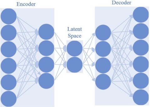
Figure 1: Autoencoder architecture.

2.2 Transformer

A transformer is a neural network model, which relies on attention mechanisms, dispensing with recurrent and convolutional networks entirely. This model is highly parallelizable, requiring significantly less training and testing time. Prior to the introduction of the transformer model, recurrent neural networks, such as long short-term memory (LSTM) [17] and gated recurrent unit (GRU) [18] were mainly used for sequence modeling. Due to their power in sequence modeling and understanding the temporal relations, their slow performance was neglected. Their operation is based on receiving a data point at each time step as the input and generating a sequence of hidden states as a function of the previous hidden states and the input. This procedure does not easily render itself to parallelization, which is a challenge when these models are used for long sequences as time and memory become severe constraints. In the transformer model, time hierarchy is eliminated. In time series, the order of the data points is very important. Hence, transformer uses positional embedding to keep track of the order, and at the same time, benefits from advantages of parallelization. The attention-based architecture in our proposed model has the same essence as the conventional transformer model, as it uses both the positional embedding and the multi-head attention. However, it has significant architectural differences, such as using a pruned decoder and a pooling layer. Fig. 2 depicts the overall architecture of the proposed modified transformer model.

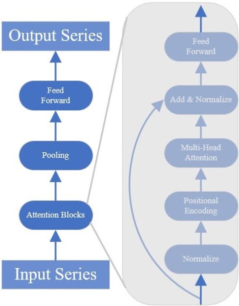
Figure 2: The proposed transformer architecture.

The proposed method in this paper does not consist of any recurrent or convolutional neural networks to pave the way for parallel computation and benefits from attention mechanism to better capture the temporal relations. In the following, some of the research works will be discussed. In Wang et al. [19], an improved LSTM block is proposed and its performance in timeseries forecasting is assessed compared to LSTM original block and GRU block. Since the proposed LSTM block achieves better forecasting performance, it is used to calculate the forecasting error and detect anomalies with forecasting. The proposed block is tested on rail transit operation data. In Ashraf et al. [20], a neural architecture consisting of LSTM blocks in an auto-encoding arrangement is proposed which is trained on clean data and detects anomalies based on reconstruction error. The network learns allowable patterns in the clean data and detects anomalies whenever the reconstruction error exceeds a threshold. The proposed model is tested on smart transportation data such as in-vehicle communication and intrusion are modeled as an anomaly.

3 The Proposed Method

3.1 Model Operation

Let us consider a time series $X=\{x_{1},x_{2},…,x_{n}\}$, where $x_{i}\in\mathbb{R}$ is an $m$-dimensional reading at the $i$th time step that contains information of $m$ channels. The model is trained on widows of the train time series with a size of $W$. The training data should be from normal data with no anomalies. For training, the data is divided into windows of size $W$ starting from the first data point, which gives us $(n-W+1)$ windows of data points. The AE model is trained on all of the windows of data. The weights are adjusted to minimize the mean average error of the output of the decoder. The attention model operates in a way to forecast the next step in the latent space of the AE. It is trained on encodings of the AE; in every time step, its input is the encoding of the $t$th window, and its output should be the encoding of the $(t+1)th$ window. The weights are adjusted to minimize the mean average error of the current and the next time-step windows.

In order to achieve better and faster convergence in model training and the ability to use the model for a broader range of datasets, data is normalized. The data is normalized based on the minimum and maximum of the training data. Then, to normalize the rest of the data, we use the same minimum and maximum. After the training of the model, the function of the model can be summarized as follows:

• The window of new data is fed into the encoder of the AE:

  $Encoder(x_{1}^{t},x_{2}^{t},…,x_{W}^{t})$

• The encoded window is in the latent space of the AE and is fed to the attention model, and the attention model predicts the encoding of the next step window:

  $Transformer(Encoder(x_{1}^{t},x_{2}^{t},…,x_{W}^{t}))$

• The prediction is decoded and marked as the model’s prediction of the next time-step window:

  $Prediction=Decoder(Transformer(Encoder(x_{1}^{t},x_{2}^{t},…,x_{W}^{t})))$

• Reconstruction error is calculated and appended to the error list:

  $Error=(x_{1}^{t+1},x_{2}^{t+1},…,x_{W}^{t+1})$ – $Prediction$

• At each time step, the algorithm calculates an average of the error list. If the calculated error is more than average for a few consecutive time steps, it detects the time step as an anomaly.

After training the model, it learns the temporal relationships; therefore, it is expected that if an anomaly from any of the three mentioned types happens in a window, there would be a jump in that window’s reconstruction error for a few consecutive time steps. Fig. 3 depicts the schematic diagram of the model.

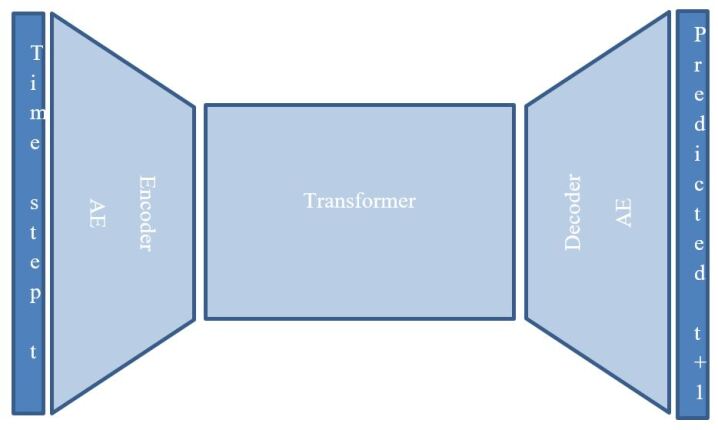
Figure 3: Schematic of the proposed model for anomaly detection.

Some anomaly models use a threshold as a criterion for detecting an anomaly [7], but checking if the error is more than average for a few consecutive time steps is more accurate, because this pattern repeats specially for collective and contextual anomalies. Next section covers the implementation details and the obtained results on a number of benchmark time series.

3.2 Model Training

3.2.1 Autoencoder Training

The autoencoder undergoes training on clean data within the primary $n$-dimensional space. Given its objective of reconstructing windows, the choice of loss function is pivotal, typically manifesting as either mean squared error (MSE) or mean absolute error (MAE). The autoencoder training process is demonstrated in Algorithm 1.

Algorithm 1 Autoencoder Training

1:Input: Time series $X=\{x_{1},x_{2},…,x_{n}\}$, window size $W$

2:Preprocess Data: Normalize $X$ based on training data

3:Initialize: Autoencoder Model (AE) parameters

4:Training:

5:for $t\leftarrow 1$ to $(n-W+1)$ do

6:     $window_{t}\leftarrow(x_{t},x_{t+1},...,x_{t+W-1})$

7:     $encoded\_window_{t}\leftarrow\text{AE.Encoder}(window_{t})$

8:     $predicted\_window_{t}\leftarrow\text{AE.Decoder}(encoded\_window_{t})$

9:     Compute loss and update AE parameters using backpropagation

10:end for

3.2.2 Transformer Training

The improved transformer is subjected to training within the $m$-dimensional ($m<n$) latent space of the autoencoder, utilizing clean data. Its primary goal is the prediction of the succeeding window within the latent space of the autoencoder. A comprehensive demonstration of the transformer training process is presented in Algorithm 2.

Algorithm 2 Transformer Training

1:Input: Time series $X=\{x_{1},x_{2},…,x_{n}\}$, window size $W$

2:Preprocess Data: Normalize $X$ based on training data

3:Initialize: Autoencoder Model (AE), Transformer Model (Transformer) parameters

4:Training:

5:for $t\leftarrow 1$ to $(n-W)$ do

6:     $window_{t}\leftarrow(x_{t},x_{t+1},...,x_{t+W-1})$

7:     $encoded\_window_{t}\leftarrow\text{AE.Encoder}(window_{t})$

8:     $predicted\_encoded\_window_{t}\leftarrow\text{Transformer}(encoded\_window_{t})$

9:     $target\_encoded\_window_{t+1}\leftarrow\text{AE.Encoder}(x_{t+W})$

10:     Compute loss and update Transformer parameters using backpropagation

11:end for

4 Results

This section presents the experimental results obtained by the proposed model based on six real-world datasets; the internal temperature of an industrial machine, Amazon Web Services (AWS) cloud watch data for Relational Database Service (RDS) and Elastic Compute Cloud (EC2), average CPU usage across a given cluster from AWS CPU usage monitoring, real traffic data (occupancy) from the Twin Cities Metro in Minnesota, and number of Twitter mentions of Google. All of the datasets were retrieved from Numenta Anomaly Benchmark (NAB) [19]. These datasets are carefully chosen to demonstrate the ability of our proposed model in anomaly detection for datasets with various real-world sources as well as all types of anomalies, for instance, contextual and collective anomalies are observed in machine temperature and CPU utilization datasets and point anomaly is observed in AWS EC2 dataset. In the experiments, all of the predicted anomalies, which lie in the dataset’s labeled anomaly window as true positives, were counted.

Table 1: Results achieved by the proposed model for different time series

Dataset	Window Size	Precision	Recall	F1 Score
Machine Temperature	90	98.0%	100%	99.0%
CPU Utilization	50	100%	100%	100%
AWS RDS	90	96.4%	100%	98.2%
AWS EC2	70	96.2%	100%	98.1%
Google’s Tweet Volume	70	93.1%	100%	96.4%
Traffic Occupancy	70	100%	100%	100%

In the experiments, two anomaly detection algorithms were used and evaluated based on their reconstruction errors. The first algorithm is based on the pattern, which is repeated at every anomaly. It is more reliable for contextual and collective anomalies and is able to operate even without validation data. It checks if the difference between the calculated errors in the last two steps is more than the average reconstruction error in the previous steps. The preceision of this algorithm is increased as it is used for more consecutive error pairs. This algorithm is used for anomaly detection in machine temperature, CPU utilization, traffic occupancy, and AWS RDS datasets. Since anomalies in these datasets are mostly contextual or collective. The second algorithm uses a specific number determined by validation data as a threshold to announce a point as an anomaly, if its reconstruction error is more than the specified threshold. This method needs validation data to determine the threshold and works best for point anomalies, and has a weaker performance in detecting contextual and collective anomaly types. Table 1 demonstrates the accuracy achieved by the proposed algorithm for different time series using the mentioned prediction window size. Fig. 4 demonstrates the proposed model’s predictions, anomaly points, and anomaly windows labeled in the datasets.

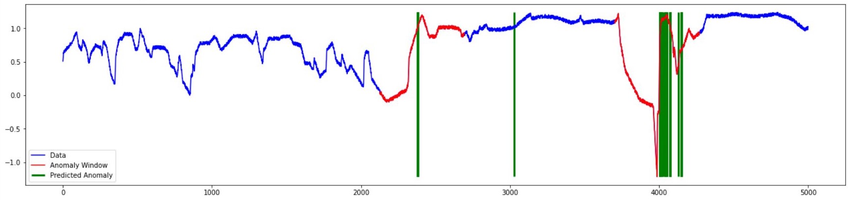
(a) Machine Temperature Dataset

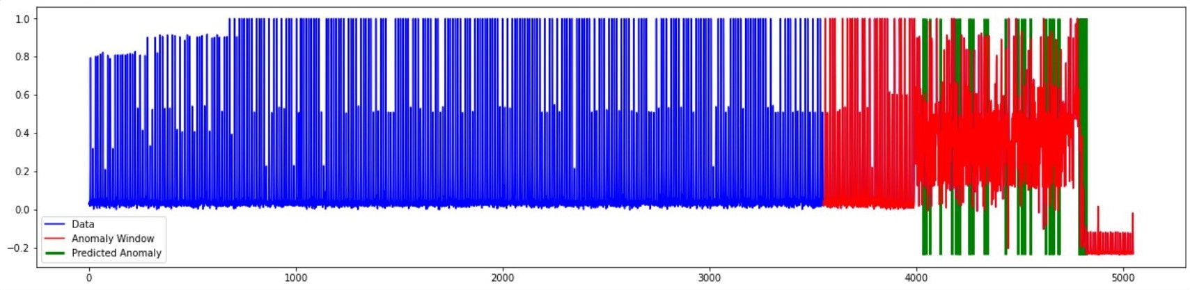
(b) CPU Utilization Dataset

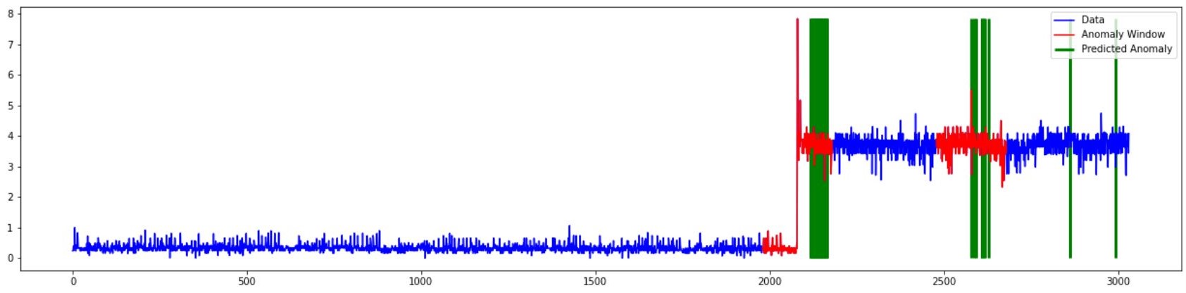
(c) AWS RDS Dataset

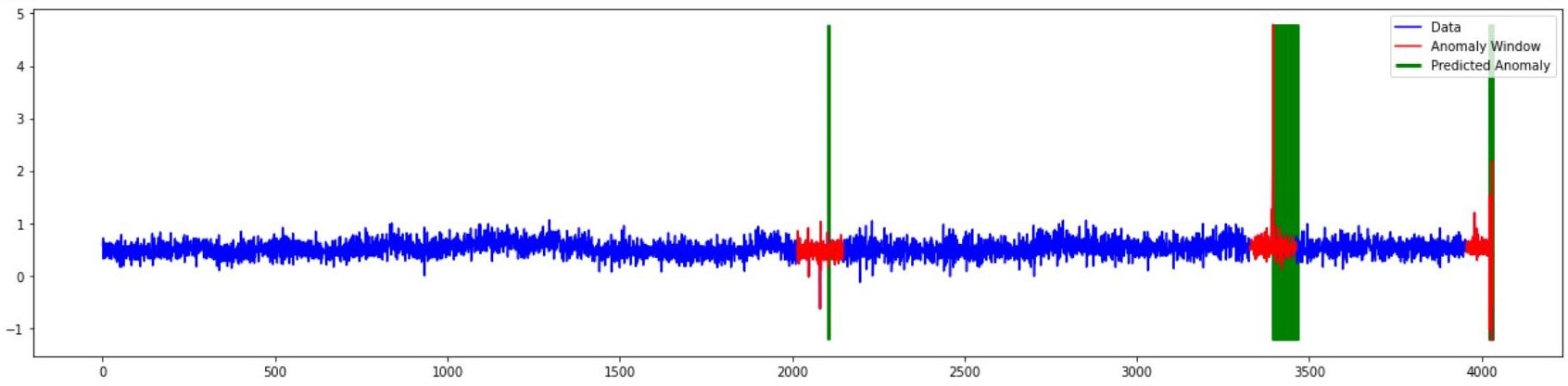
(d) AWS EC2 Dataset

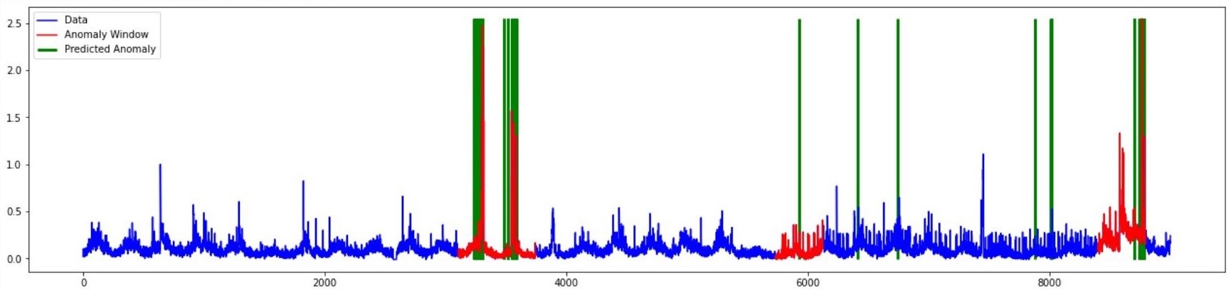
(e) Google’s Tweet Volume Dataset

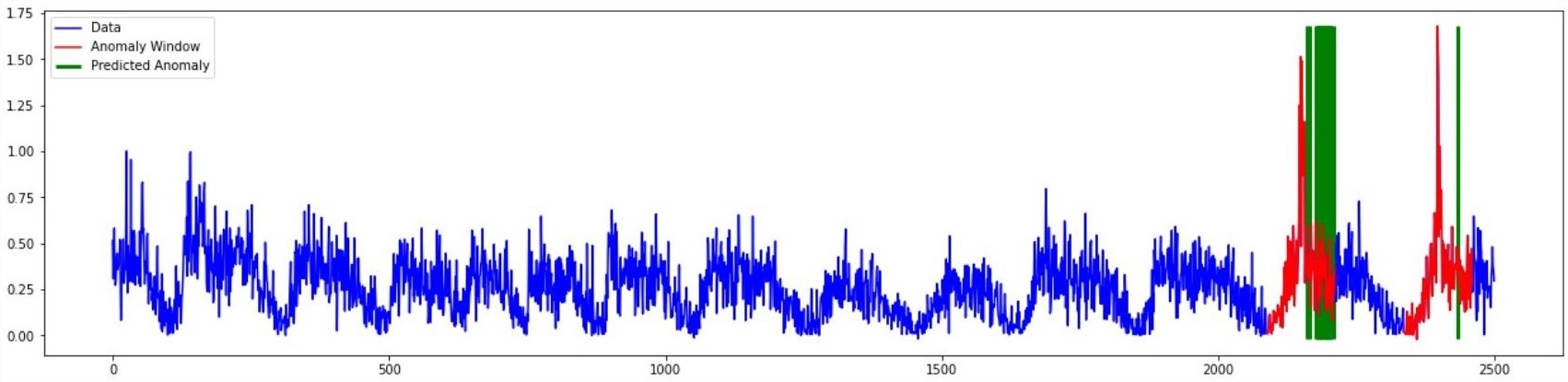
(f) Traffic Occupancy Dataset

Figure 4: Experimental results for different time series.

According to Table 1 and Fig. 4, the proposed model shows promising results in detecting all three types of anomalies. Moreover, most of the false positives announced by our model have considerable differences from other normal points in the time series. However, they are not labeled as anomalies in the datasets. Our model detects all of the anomalies in all six datasets and performs with the highest precision in two of them. Its lowest precision occurs in Google’s Tweet Volume Dataset, which is 93.1%. The reason might be the anomalous patterns that are repeated throughout this dataset. Table 2 compares the proposed model with four other well-established deep models. The proposed model outperforms all of them for two of the datasets with a wide margin, while losing to only one of them for the third dataset with a narrow margin of 1.5% in F1 Score.

Table 2: Comparison between different anomaly detection algorithms applied to different time series

Dataset	Model	Window Size	Precision	Recall	F1 Score
	Proposed method	90	98.0%	100%	99.0%
	VAE-LSTM [7]	288	55.9%	100%	71.7%
Machine Temperature	VAE [20]	48	21.1%	100%	20.7%
	LSTM-AD [21]	48	100%	50.0%	66.7%
	ARMA [22]	48	14.2%	100%	24.8%
	Proposed method	50	100%	100%	100%
	VAE-LSTM [7]	144	69.4%	100%	81.9%
CPU Utilization	VAE [20]	24	34.8%	50.0%	41.0%
	LSTM-AD [21]	24	27.4%	100%	43.0%
	ARMA [22]	24	23.4%	100%	38.0%
	Proposed method	70	96.2%	100%	98.1%
	VAE-LSTM [7]	192	99.3%	100%	99.6%
AWS EC2	VAE [20]	24	94.9%	100%	97.4%
	LSTM-AD [21]	24	100%	43.6%	60.8%
	ARMA [22]	24	93.8%	100%	96.8%

Because of its unique architecture and absence of recurrent and convolutional layers in our proposed model, it is highly computationally parallelizable. Therefore, deploying a GPU in training or employing it would boost its performance and make it a suitable choice for real-time applications. As a testify, in training the model on EC2 dataset with 1700 time steps of normal training data using Google Colab’s Tesla T4 GPU, each epoch of autoencoder training roughly takes 0.15 seconds on GPU while taking 0.18 seconds without GPU. The gap is way more significant for training the attention-based model, as it takes about 20 seconds for each epoch on GPU and takes about 860 seconds in training without GPU. The autoencoder converges after about 500 epochs, while the attention-based model needs only five epochs to converge.

5 Conclusion

In this work, we proposed an attention-based and autoencoder hybrid model as a solution for unsupervised anomaly detection in time series. Our proposed method benefits from an autoencoder to learn the local features and to summarize the windows into short embeddings used by the attention-based model as input. The attention-based model is built on the transformer model [8] with major architectural differences, such as deploying a pooling layer and a pruned decoder. The attention-based architecture is used to model long-term temporal relations. The proposed model does not use recurrent or convolutional layers. Hence, it renders itself to parallel computation, which in turn expedites the training process and reduces the computation time in using the trained model. This paves the way for using the proposed algorithm in real-time tasks. The proposed algorithm was applied to six different real-world datasets from the NAB anomaly detection benchmark, and its performance was compared with five well-established models. Results confirmed the effectiveness of the proposed architecture for unsupervised online anomaly detection.

References

- [1] Luo, Y., Xiao, Y., Cheng, L., Peng, G. and Yao, D., 2021. Deep learning-based anomaly detection in cyber-physical systems: Progress and opportunities. ACM Computing Surveys (CSUR), 54(5), pp.1-36.
- [2] Inoue, J., Yamagata, Y., Chen, Y., Poskitt, C.M. and Sun, J., 2017, November. Anomaly detection for a water treatment system using unsupervised machine learning. In 2017 IEEE international conference on data mining workshops (ICDMW) (pp. 1058-1065). IEEE.
- [3] Wang, Y., Masoud, N. and Khojandi, A., 2020. Real-time sensor anomaly detection and recovery in connected automated vehicle sensors. IEEE transactions on intelligent transportation systems, 22(3), pp.14111421.
- [4] Yin, C., Zhang, S., Wang, J. and Xiong, N.N., 2020. Anomaly detection based on convolutional recurrent autoencoder for IoT time series. IEEE Transactions on Systems, Man, and Cybernetics: Systems, 52(1), pp.112122.
- [5] Pereira, J. and Silveira, M., 2018, December. Unsupervised anomaly detection in energy time series data using variational recurrent autoencoders with attention. In 2018 17th IEEE international conference on machine learning and applications (ICMLA) (pp. 1275- 1282).
- [6] Fahrmann, D., Damer, N., Kirchbuchner, F. and Kuijper, A., 2022.¨ Lightweight Long Short-Term Memory Variational Auto-Encoder for Multivariate Time Series Anomaly Detection in Industrial Control Systems. Sensors, 22(8), p.2886.
- [7] Lin, S., Clark, R., Birke, R., Schonborn, S., Trigoni, N. and Roberts,¨ S., 2020, May. Anomaly detection for time series using vae-lstm hybrid model. In ICASSP 2020-2020 IEEE International Conference on Acoustics, Speech and Signal Processing (ICASSP) (pp. 4322-4326). Ieee.
- [8] Vaswani, A., Shazeer, N., Parmar, N., Uszkoreit, J., Jones, L., Gomez, A.N., Kaiser, Ł. and Polosukhin, I., 2017. Attention is all you need. Advances in neural information processing systems, 30
- [9] Wu, N., Green, B., Ben, X. and O’Banion, S., 2020. Deep transformer models for time series forecasting: The influenza prevalence case. arXiv preprint arXiv:2001.08317.
- [10] Braei, M. and Wagner, S., 2020. Anomaly detection in univariate timeseries: A survey on the state-of-the-art. arXiv preprint arXiv:2004.00433.
- [11] Bank, D., Koenigstein, N. and Giryes, R., 2020. Autoencoders. arXiv preprint arXiv:2003.05991.
- [12] Kieu, T., Yang, B., Guo, C. and Jensen, C.S., 2019, August. Outlier Detection for Time Series with Recurrent Autoencoder Ensembles. In IJCAI (pp. 2725-2732).
- [13] Atashgahi, Z., Mocanu, D.C., Veldhuis, R. and Pechenizkiy, M., 2022. Memory-free Online Change-point Detection: A Novel Neural Network Approach. arXiv preprint arXiv:2207.03932.
- [14] Hasan, M., Choi, J., Neumann, J., Roy-Chowdhury, A.K. and Davis, L.S., 2016. Learning temporal regularity in video sequences. In Proceedings of the IEEE conference on computer vision and pattern recognition (pp. 733-742).
- [15] Gong, D., Liu, L., Le, V., Saha, B., Mansour, M.R., Venkatesh, S. and Hengel, A.V.D., 2019. Memorizing normality to detect anomaly: Memory-augmented deep autoencoder for unsupervised anomaly detection. In Proceedings of the IEEE/CVF International Conference on Computer Vision (pp. 1705-1714).
- [16] Zong, B., Song, Q., Min, M.R., Cheng, W., Lumezanu, C., Cho, D. and Chen, H., 2018, February. Deep autoencoding gaussian mixture model for unsupervised anomaly detection. In International conference on learning representations.
- [17] Hochreiter, S. and Schmidhuber, J., 1997. Long short-term memory. Neural computation, 9(8), pp.1735-1780.
- [18] Chung, J., Gulcehre, C., Cho, K. and Bengio, Y., 2014. Empirical evaluation of gated recurrent neural networks on sequence modeling. arXiv preprint arXiv:1412.3555.
- [19] Wang, Y., Du, X., Lu, Z., Duan, Q. and Wu, J., 2022. Improved lstmbased time-series anomaly detection in rail transit operation environments. IEEE Transactions on Industrial Informatics, 18(12), pp.90279036.
- [20] Ashraf, J., Bakhshi, A.D., Moustafa, N., Khurshid, H., Javed, A. and Beheshti, A., 2020. Novel deep learning-enabled LSTM autoencoder architecture for discovering anomalous events from intelligent transportation systems. IEEE Transactions on Intelligent Transportation Systems, 22(7), pp.4507-4518.
- [21] Ahmad, S., Lavin, A., Purdy, S. and Agha, Z., 2017. Unsupervised real-time anomaly detection for streaming data. Neurocomputing, 262, pp.134-147.
- [22] An, J. and Cho, S., 2015. Variational autoencoder based anomaly detection using reconstruction probability. Special Lecture on IE, 2(1), pp.1-18.
- [23] Malhotra, P., Vig, L., Shroff, G. and Agarwal, P., 2015, April. Long short term memory networks for anomaly detection in time series. In Proceedings (Vol. 89, pp. 89-94).
- [24] Pincombe, B., 2005. Anomaly detection in time series of graphs using arma processes. Asor Bulletin, 24(4), p.2.