Pixar: Auto-Regressive Language Modeling in Pixel Space

Abstract

Recent works showed the possibility of building open-vocabulary large language models (LLMs) that directly operate on pixel representations and are implemented as encoder-decoder models that reconstruct masked image patches of rendered text. However, these pixel-based LLMs are limited to autoencoding tasks and cannot generate new text as images. As such, they cannot be used for open-answer or generative language tasks. In this work, we overcome this limitation and introduce Pixar, the first pixel-based autoregressive LLM that does not rely on a pre-defined vocabulary for both input and output text. Consisting of only a decoder, Pixar can answer free-form generative tasks while keeping the text representation learning performance on par with previous encoder-decoder models. Furthermore, we highlight the challenges to autoregressively generate non-blurred text as images and link this to the usual maximum likelihood objective. We propose a simple adversarial pretraining that significantly improves the readability and performance of Pixar making it comparable to GPT2 on short text generation tasks. This paves the way to building open-vocabulary LLMs that are usable for free-form generative tasks and questions the necessity of the usual symbolic input representation – text as tokens – for these challenging tasks.

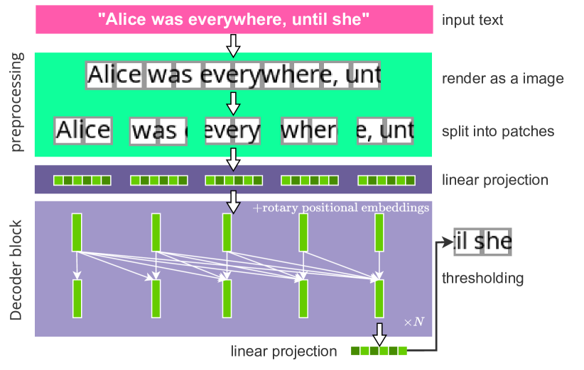
Figure 1: Pixar is the first generative language model without any embedding layers or vocabulary. Pixar accepts texts as images and also generates texts in image patches autoregressively. We can recognize the generated texts using OCR software.

1 Introduction

In the Natural Language Processing (NLP) domain, the tokenizer is an essential ingredient used to divide the raw text into a sequence of sub-units, such as sub-words (Wu et al., 2016), characters (Cui et al., 2020), sentence pieces (Kudo & Richardson, 2018), and bytes (Sennrich et al., 2016). Normally, NLP models represent those sub-units within an ID-based categorical vocabulary.

This categorical representation highlights three weaknesses of traditional NLP systems. First, to represent each item in the vocabulary, NLP systems have to allocate an embedding matrix with a number of rows that grows linearly with the size of the vocabulary. This is exacerbated in current Large Language Models that allocate millions of parameters just for this. Additionally, the data mismatch between pretraining and downstream tasks leads to out-of-vocabulary (OOV) problems and performance degradation. Tokenization with smaller granularities, such as characters and bytes, can alleviate the OOV problem but bring about longer sequence lengths and increase computational overhead (Kaddour et al., 2023). Finally, graphical information of texts in specific language is thereby ignored (Sun et al., 2021).

To tackle these problems, researchers proposed pixel-based approaches that can treat text as images by using a dedicated visual encoder to derive “token” vectors from the image patches. Pixel-based embeddings remove the need for a finite vocabulary and keep the visual information of texts. With this idea, Rust et al. (2023) proposed Pixel, which consists of an MAE (He et al., 2021) backbone trained with a masked image patch reconstruction objective. Pixel achieved comparable performance with BERT (Devlin et al., 2019) in a wide range of downstream classification and regression NLP tasks. Moreover, Pixel is observed more robust to the character-level noisy input and visual attacks (Eger et al., 2020). A downside of this approach is that the auto-encoder nature of Pixel restricts its applicability to discriminative tasks only.

Generating pixel-based text with an open-vocabulary structure is still under-explored. To fill this gap, we present Pixar, which is the first pixel-based autoregressive LLM that doesn’t require any embedding layers. Different from Pixel, Pixar consists of a transformer decoder (Vaswani et al., 2023) which takes a sequence of text image patches as inputs, and outputs image patches containing new text.

Pixar is pretrained using a 2-stage pretraining strategy. In stage 1, following previous work on autoregressive LLMs (Radford et al., 2019) and image generation models (Chen et al., 2020b), Pixar is trained using a large-scale corpus of rendered text using teacher forcing. We optimize the Pixar to minimize the reconstruction loss on a dataset similar to Pixel’s. However, models trained with only reconstruction loss tend to generate blurred images which do not contain readable words. This is potentially due to the uncertainty involved in generating the next word which may span several words which look very dissimilar.

To mitigate this problem, we proposed an additional pretraining stage, where Pixar is trained with the reconstruction loss plus a balanced adversarial loss. Our experiments in Section 6 show that 200 steps of stage 2 pretraining improves the generation readability significantly and achieves comparable performance with GPT2 (Radford et al., 2019) on open-answer short generative tasks. Also, with an equivalent amount of training steps and epochs, Pixar achieves a level of language understanding performance which is on par with Pixel while keeping the number of parameters only equivalent to the encoder part of Pixel.

Our results in both discriminative and generative tasks showcase the potential of using pixel-based autoregressive models for learning more language models that are not constrained by the original training vocabulary and that can therefore be transferred more easily to different languages and application domains.

2 Beyond token-based LLMs

The idea of using pixel-based representation has long existed in NLP research. It was initially applied for Chinese due to its graphic feature. Liu et al. (2017) used a CNN-based block to extract character-level visual representations. Similarly, Sun et al. (2018) rendered Chinese sentences into fixed-size images and used a CNN network for text classification tasks. Meng et al. (2020) exploited the Tianzige feature of Chinese characters and also applied a CNN layer to capture graphic information and combine it with traditional ID-based embeddings as a mixed input of RNN-based models. Later, Dai & Cai (2017) and ChineseBERT (Sun et al., 2021) explored using character-level visual features for BERT-based models. The idea of using character-level visual features is not limited to pixel-based models. For instance, MacBERT (Cui et al., 2020) and Jozefowicz et al. (2016) also used character-level encodings however they still relied on traditional ID-based embeddings thus suffering the vocabulary bottleneck problem.

Inspired by how OCR models work, Pixel (Rust et al., 2023) reused the MAE (He et al., 2021) architecture and rendered text as images therefore trained to reconstruct masked text image patches. Therefore, Pixel is capable of accepting any text input avoiding the OOV problem by design. Pixel-based representation is also been used as input representation for generative tasks. Salesky et al. (2021) and Salesky et al. (2023) build machine translation models with an encoder-decoder structure and accept visual information as input. However, their output layers still rely on embedding layers with a fixed vocabulary. GlyphDiffusion (Li et al., 2023a) made attempts to use a diffusion model to generate new texts as images from noise and conditioned on encoded text features. However, the text encoder of GlyphDiffusion relies on embedding layers and thus still suffers from the vocabulary bottleneck problem. The cascaded diffusion model also brings large computational overhead while inference.

Alternatively, byte-level tokenization is also capable of encoding any code sequence. Xue et al. (2021) trained mT5 on UTF-8 byte sequence to adapt to different languages. Perceiver (Jaegle et al., 2021) proposed an iterative transformer structure which attends information directly through raw byte arrays. However, byte-level encoding significantly prolongs the input sequence length when trained on unseen texts and increases computational overhead (Kaddour et al., 2023).

3 Pixar

Motivated by our aim to create a model that can understand and generate natural language without the problems of traditional NLP systems, we follow Pixel and leverage pixel-based representations as our representation for natural language. In this paper, we propose a novel architecture that generalises Pixel that abandons the auto-encoder architecture of MAE and instead applies the design choices of other generative LLMs like LLaMA (Touvron et al., 2023a, b). In this way, we can pretrain Pixar with the next patch prediction objective, which aligns with the next token prediction training used for other generative LLMs.

3.1 Text Rendering

To convert the text data into images, we use the same PangoCairo render from Rust et al. (2023) to render text as images. For better readability under a low resolution, we choose the pixel-style font “Pixeloid Sans ”. For binary images, we render each pixel to a gray-scale value first then threshold each pixel value to 0 or 1 corresponding to black and white. For continuous RGB images, we map each pixel value to the [-1, 1] interval without normalization. We follow Rust et al. (2023)’s implementation that uses a black patch to represent special EOS tokens. For downstream tasks with text pairs, we also use a black patch as the delimiter.

3.2 Model Architecture

We built Pixar as a transformer decoder-only model. Unlike other language models, Pixar does not have embedding layers but directly takes image patches as input and projects them into vector representations. Similar to the implementation of Rust et al. (2023), for an image patch $\boldsymbol{x}\in\mathbb{R}^{H\times W\times C}$, we first flatten all pixel values into a vector, then project it into a hidden embedding $h_{\text{in}}\in\mathbb{R}^{d_{\text{model}}}$, where $d_{\text{model}}$ is the hidden dimension of the transformer backbone. Therefore, we feed these hidden embeddings as the input of the first transformer decoder layer.

The transformer decoder layer of Pixar is similar to LLaMA’s structure (Touvron et al., 2023a). We added rotary positional embeddings (Su et al., 2023) at each layer of the network and applied the SwiGLU activation function (Shazeer, 2020).

To output image patches, we reverse the input procedure. For each generated hidden embedding $h_{\text{out}}$ from the last transformer layer, we project it to a vector with a dimension equal to the number of pixel values within a patch, then reshape it into an image patch $\boldsymbol{\hat{x}}$. When predicting binary images, we calculate the probability of being white for each pixel by applying an element-wise sigmoid function

$$P_{\text{white}}=\sigma(\boldsymbol{\hat{x}}/T)$$

where $T$ is the temperature parameter. When visualizing, we can either render the output image patches as grey-scale images using the probability value of each pixel or threshold them into black or white. When generating RGB images, we directly map output values to pixel values of each channel. From a probabilistic viewpoint, our model approximates a Gaussian distribution of pixel values with constant variance. And we use the mode of each predicted Gaussian distribution as the pixel values while visualizing.

Similar to other decoder-only models, like GPT2 or LLaMA, Pixar is also pretrained using the teacher-forcing strategy. We applied the causal masking strategy to prevent hidden embeddings from attending to future visual patches. During the pretraining, we used MSE loss for models with RGB images and Cross-entropy loss for binary image models, where the temperature of the sigmoid function is set to 1.

3.3 Applications

As previously mentioned, Pixar generalises the architecture of Pixel and allows us to assess its performance on both discriminative and generative tasks. Depending on the task, we use Pixar’s learned representations in different ways that we describe below.

Classification & Regression We can add a lightweight task head to Pixar to make it output classification labels or regression scores. For classification tasks, the task head is a linear projection layer followed by a softmax function to output the probability of each class. For regression tasks, the task head is only a linear projection layer that directly outputs a scalar value as the desired score.

Because of the causal masking strategy, only the last “token” could attain all information of the input sequence. We therefore only feed the EOS token’s embedding to the task head.

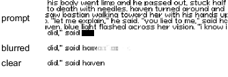
Figure 2: The stage 2 adversarial training improves the readability significantly. The blurred sample is generated by Pixar with only stage 1 pretraining and the clear sample is generated from that model with 200 steps of stage 2 adversarial pretraining. The prompt is from the LAMBADA test set.

Generation Pixar can autoregressively generate the next image patch and append the generated patch to the end of the input sequence repeatedly. When evaluating the generation quality, we can use arbitrary OCR software to recognize texts from generated images. Then calculate the corresponding metrics on the recognized texts.

However, as Figure 2 shows, because Pixar trained with only reconstruction loss tends to generate blurred images which do not contain readable texts. We also defined a readability metric to measure the text generation quality.

model	$|\theta|$	MNLI-m/mm	QQP	QNLI	SST-2	COLA	STSB	MRPC	RTE	WNLI	AVG
		392k	363k	108k	67k	8.5k	5.7k	3.5k	2.5k	635
BERT	110M	84.0/84.2	87.6	91.0	92.6	60.3	88.8	90.2	69.5	51.8	80.0
Pixel	86M	78.1/78.9	84.5	87.8	89.6	38.4	81.1	88.2	60.5	53.8	74.1
Pixar	85M	78.4/78.6	85.6	85.7	89.0	39.9	81.7	83.3	58.5	59.2	74.0

Table 1: Pixar achieves on-par performance with Pixel on GLUE validation set. Pixar achieved this performance with fewer parameters and a simpler structure compared with the encoder-decoder structure of Pixel. We report the F1 score for MRPC and QQP, Matthew’s correlation for COLA, Spearman’s $\rho$ for STSB, and accuracy for other tasks. We report BERT performance here as a reference. Scores of BERT and Pixel are originally reported in Rust et al. (2023). The best performance of each task is marked in bold.

3.4 Readability Metric

To measure the readability of model generation, we quantitatively count the ratio of generated image patches that contain at least one leading English word. While assessing, we concatenate a sequence of generated image patches into one image and use OCR software to recognize the text within it. Because the first generated word should be located at the beginning of the image patch, we only treat the image patch with English words at the beginning of the OCR result. In this research, we used 333k most common English words from the English Word Frequency dataset from Kaggle to evaluate the readability.

4 Challenges in Generating Readable Text

During stage 1 pretraining, the model is trained to maximize the log-likelihood by optimizing the KL divergence. However, we observe that the model tends to generate blurred or noisy images due to the mismatch between the real distribution and the modeled distribution. As Figure 2 shows, it’s hard for people to read from blurred or noisy images. An intuition is that because of several possible semantically close candidate words look very dissimilar. For example, the next word of “Today is ” might be “sunny” with 0.4 probability and “rainy” with 0.6 probability, but the model tends to generate an image patch with 0.4 “sunny” and 0.4 “rainy” stacked up.

4.1 Adversarial Training

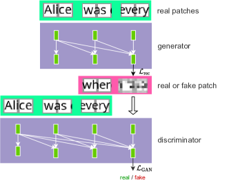
Figure 3: We copied the Pixar from stage 1 pretraining as both the generator and the discriminator for the adversarial training in stage 2. The generator is optimized by both reconstruction loss $\mathcal{L}_{\text{rec}}$ and adversarial loss $\mathcal{L}_{\text{GAN}}$ to improve the generation readability.

To improve the readability, we proposed a second-stage adversarial training (Esser et al., 2021). In the first stage, Pixar is only optimized to minimise the reconstruction loss $\mathcal{L}_{\text{rec}}$ but leads to blurred images as Figure 2 shows. To mitigate this problem, we pretrain the model to minimize an adversarial loss in the second stage. Our experiments in 6.2 show a 200-step short stage two training boosts the readability and generation performance.

Pixar as Discriminator In the second stage, the adversarial loss makes Pixar become a generative adversarial model (GAN) (Goodfellow et al., 2014). To construct the discriminator, we append a patch-wise classification head to Pixar. For a sequence $\boldsymbol{x}_{1:i}$, the discriminator is trained to decide whether $\boldsymbol{x}_{i}$ is generated or real conditions on real previous patches $\boldsymbol{x}_{1:i-1}$.

A naive approach to calculate the adversarial loss is passing all subsequences $\{\boldsymbol{x}_{1:j};j\leq i\}$ with real or fake $\boldsymbol{x}_{j}$ to the discriminator. However, this approach multiplies the computational overhead by the length of the sequences.

We exploit the cached key and query vectors to improve the computation efficiency. We first calculate all key and query values of the real sequence $\boldsymbol{x}_{1:i}$ and cache them as $C_{1:i}$. Then the model classifies the generated patch $\hat{\boldsymbol{x}}_{j}$ conditioned on $C_{1:j-1}$. To further simplify the computation, we only sample 30 fake patches from 1 sequence. Since the classification of real patches could be calculated from the cached vectors, we used all real patches.

Balanced Adversarial Loss GAN is notorious for its training instability. In the second stage, we used a balanced loss ratio which is inspired from Esser et al. (2021). The generator’s target is to minimize both the reconstruction loss $\mathcal{L}_{\text{rec}}$ and the GAN loss $\mathcal{L}_{\text{GAN}}$. We balance them by multiplying a manually picked weight $\lambda$ and an automatic ratio to the GAN loss. Thus, the total loss of the generator could be written as

$$\mathcal{L_{G}}=\mathcal{L}_{\text{rec}}+\lambda\frac{\nabla_{G_{L}}[\mathcal{L}_{\text{rec}}]}{\nabla_{G_{L}}[\mathcal{L}_{\text{GAN}}]+\delta}\mathcal{L}_{\text{GAN}}.$$

The operator $\nabla_{G_{K}}[\cdot]$ represents the scale of gradients of its input w.r.t to the last layer $L$ of the generator, and $\delta=1e^{-8}$ is added to avoid zero divisors.

Combining discriminator’s classification loss $\mathcal{L}_{D}$, the complete training target of stage two is to find the Nash equilibrium (Osborne & Rubinstein, 1994)

$$\theta_{G}^{*}= \operatorname*{arg\,min}_{\theta_{G}}\operatorname*{arg\,max}_{\theta_{D}}\mathbb{E}_{\boldsymbol{x}_{1:i}\sim P}[\mathcal{L}_{\text{rec}}-$$

$$\lambda\frac{\nabla_{G_{L}}[\mathcal{L}_{\text{rec}}]}{\nabla_{G_{L}}[\mathcal{L}_{\text{GAN}}]+\delta}\mathcal{L}_{\text{GAN}}].$$

During the training, both $\theta_{G}$ and $\theta_{D}$ are optimized together in each step.

5 Related Work

5.1 Generative Language Models

Language models learn to predict probability distributions over a sequence of input elements which can have different granularity including words, tokens, characters, or pixels, which is the approach we follow in this work. This task is generally referred to as next token prediction and it represents a crucial problem in natural language processing (Shannon, 1948). The advent of transformers brought about a huge improvement in this field, especially in parallel training and capturing long-range dependencies (Vaswani et al., 2023). Surprisingly, the family of generative pre-trained transformers (Radford et al., 2019; Brown et al., 2020; Workshop et al., 2023; Touvron et al., 2023a, b; Penedo et al., 2023) demonstrated their strong ability to understand and generate natural language.

5.2 Transformer-based Image Generative Models

The task of image generation can be formulated as pixel-based autoregressive modeling. In the literature, this task was attempted using different architectures such as CNNs (Salimans et al., 2017), RNNs (van den Oord et al., 2016) and Transformers (Chen et al., 2020a; Menick & Kalchbrenner, 2018). However, the method of generating only 1 pixel at each step is limited to low-resolution images but not high-resolution images due to long sequence lengths and poor fidelity. Also, the sequential generative modeling and teacher-forcing training of generative transformers are not suitable for flattened image vectors since they learn to predict the probability distribution over a fixed finite vocabulary instead of image patches.

To mitigate this issue, a two-stage approach is proposed to learn a Vector-Quantized Variational Autoencoder(VQ-VAE) (van den Oord et al., 2018) to map continuous pixel values into a sequence of discrete tokens and then use a transformer decoder to model the distribution of the latent image tokens. This two-stage image tokenization approach not only contributes to generative modeling for high-fidelity images (Chang et al., 2023, 2022; Ramesh et al., 2022; Tschannen et al., 2023) but also shed the way for interleaved multimodal generation by simply concatenating the vocabularies for both text and images (Aghajanyan et al., 2022, 2023). Learning from the discrete latent space of VQ-VAE becomes a popular way for models to improve image generation quality and enable language-inspired self-supervised learning (Bao et al., 2022; Li et al., 2023b).

6 Experiments

6.1 Pretraining

We used a similar pretraining dataset as Pixel. The pretraining dataset is a composite of Bookcorpus and a dump of English Wikipedia. As Table 4 shows, there are 6.5M Wikipedia articles and 0.2M books in total. However, directly rendering a book or a Wikipedia article as a training sample will waste a lot of text because they are much longer than the context window.

Therefore, to improve data utility, we split each article or book into several shorter samples. Firstly, we use the “PunktSentenceTokenizer” from the Natural Language Toolkit (NLTK) (Bird et al., 2009) to segment each article or book into sentences. Then, we concatenate short sentences to training samples within a character limit. Finally, we filter out samples with less than 100 characters. The detailed preprocessing is demonstrated in the Appendix A.

During the pretraining, we fix the window size of Pixar as 360 patches. Thus, the model trained with a longer patch length can process more texts in each forward pass. We manually selected 1180 as the character limit for patch length 2. Table 4 demonstrates the length statistics of processed data.

In stage 1, Pixar is optimized by the AdamW optimizer (Loshchilov & Hutter, 2019) for 1M steps and the batch size is set to 384. Pixar iterated the pretraining dataset for 14.4 epochs. During the training, we linearly warmed up the learning rate to a peak value of 3e-4 in the first 2000 steps and then annealed the learning rate to 3e-6 using a Cosine scheduler (Loshchilov & Hutter, 2017). For discriminative tasks, we pretrained a Pixar with 85M parameters, which is equivalent to the encoder of the Pixel. For generative tasks, we used a Pixar with 113M parameters instead to have a comparable size with GPT2. We report details of pretraining and model architecture hyperparameters in the Appendix B.

6.2 Generative Tasks

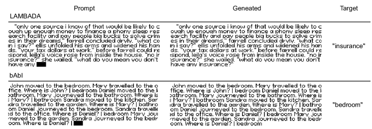
Figure 4: Pixar can generate readable and correct texts according to the prompt. We folded images into rectangles for better visibility.

Model	$|\theta|$	LAMBADA	bAbI
GPT2	124M	17.1	26.8
$\textsc{Pixar}_{\text{stage1}}$	113M	5.7(54.8)	11.1(63.2)
$\textsc{Pixar}_{\text{stage2}}$	113M	13.8(82.2)	19.6(77.0)

Table 2: Pixar with a 2-stage pretraining is comparable with GPT2 on short generative tasks. We report the zero-shot last word prediction accuracy of the LAMBADA test set and the few-shot accuracy of 10K synthesized bAbI task 1 samples. We also included the readability ratio in the round parentheses.

We render the prompt into an image and fix the white space at the right end as 3 pixels long. Then Pixar generates the next image patches autoregressively after the prompt. To recognize the generated texts, we only input the generated patches to the OCR software. Figure 4 shows some generation samples of LAMBADA (Paperno et al., 2016) and bAbI (Weston et al., 2015). We displayed more samples in Figure 5.

However, OCR software is more dedicated to images with continuous values and higher resolution. Directly applying OCR on binary images leads to erroneous recognition even if they are readable by humans. To improve the OCR accuracy, we scale the generated image patches by a factor of 3 and place them in the middle of a square white image. Also, we combine the results of two OCRs, the PaddleOCR and Tesseract OCR. If the recognized word from any of the OCRs matches the results, we count it as a correct prediction.

LAMBADA is a benchmark designed to evaluate the text-understanding capability of language models. Models need to predict the last word of a sentence in a given context. It requires the model to capture long-range dependencies and also tracks information in a broader discourse not limited to local context. During the evaluation, we only exposed the local context to models. From Table 2 we can observe that the 200 steps stage 2 pertaining boosts the model performance and the generation readability. Although Pixar cannot beat GPT2, considering that our model is 27% smaller than GPT2 and the complexity of generation, our experiments still shed light on the possibility of open-vocabulary generative language models.

bAbI is a question-answering (QA) task that evaluates the model’s inference ability based on given facts. It consists of a series of tasks of different complexity levels. Because Pixar and GPT2 are not directly trained on QA data, we show the model several examples in the prompt and split the question and answer using the “|” symbol. Table 2 shows the 200 steps stage 2 pertaining also significantly improved the accuracy and readability and achieved a comparable performance with GPT2, displaying the capability of the few-shot learning ability of Pixar.

6.3 Discriminative Tasks

We evaluated the language understanding ability of Pixar on the GLUE (Wang et al., 2018) benchmark. GLUE consists of 8 classification tasks and 1 regression task. For each task, we finetune the pretrained Pixar with a newly initialized task head on rendered data. The rendering configuration is the same as the pretraining. In some tasks, a sample consists of a pair of sentences. We inserted a black patch in between to separate them. As we discussed in 3.3, we used the embedding from the last black patch as the input of the task head.

We select the finetuning hyperparameters based on the number of training samples for each task. All tasks are trained with an evaluation frequency and the validation scores are picked from an early-stopping strategy. For tasks with more than 300k samples, e.g. MNLI and QQP, we set the maximum training step as 8000 and batch size as 256. We found that Pixar is robust to hyperparameters on tasks with more data and sensitive to batch size or learning rate for small tasks. We tried different batch size from [32, 64, 128] for STSB, RTE, and MRPC. For MRPC, we also searched different learning rate from [$1e-5$, $3e-5$, $6e-5$]. We attach the detailed hyperparameters in appendix C. Because of the resource limitation, we left the exhaustive hyperparameter searching for future work.

We finetuned on the training set and evaluated the performance on the validation set. Table 1 shows that Pixar achieved on-par performance with Pixel without the necessity for the image decoder during pretraining and with fewer parameters. Pixel is a 112M encoder-decoder model but only the 86M encoder is used for GLUE. Pixar is a decoder-only model and contains only 85M parameters, which is equivalent to the size of Pixel encoder.

Embedding	CNNAutoencoder			Linear projection
Image type	Binary	Binary	RGB	RGB	Binary	Binary	Binary
Patch length	5	2	2	2	2	5	1
MNLI-m/mm	72.5/74.1	75.8/76.2	75.8/76.4	74.9/76.3	76.4/77.6	72.5/74.0	76.2/76.3
QQP	81.2	87.8	83.4	83.5	84.3	82.1	84.0
QNLI	82.4	84.3	84.1	83.5	84.2	82.8	83.3
SST-2	83.3	86.2	86.2	86.6	88.0	82.6	87.6
COLA	15.2	30.5	26.6	30.4	27.7	16.7	39.6
STSB	69.2	74.2	74.7	73.5	81.2	71.5	73.9
MRPC	81.2	83.4	82.9	81.8	82.5	82.7	71.3
RTE	57.0	59.6	56.3	54.9	58.5	61.7	53.8
WNLI	57.7	56.3	57.7	56.3	56.3	56.3	57.7
AVG	67.4	71.4	70.4	70.2	71.6	68.3	70.4

Table 3: Pixar trained with binary data, linear projection, and patch length 2 achieved the best GLUE performance in our ablation tests where we compare variants pretrained and finetuned (only stage 1) with 0.1M steps and 113M parameters with identical hyperparameter selected heuristically as described in Section 6.3 . We therefore select the best setting for 1M pretraining .

7 Ablation and Analyses

In our preliminary experiments, we explored several design choices for a Pixar with 113M parameters, including different patch lengths, CNN-based projection layers, and the different formats of data. Because of the resource limitation, we did not exhaustively search all possible combinations. For each setting, we conducted 0.1M stage 1 pretraining steps and finetuned on the GLUE benchmark using the same hyperparameters.

7.1 Patch Length Selection

In this research, the height of image patches is fixed at 8 pixels and we render all texts as a long image with 8 pixels high. Thus, the length of each patch defines how many characters or words a patch can hold and also determines the complexity of predicting the next patch.

We pretrained models on images with patch length [1, 2, 5] for 0.1M stage 1 steps. The results in table 3 shows that in all combinations, patch length 2 achieved the highest average score. Thus, we used patch length 2 in the longer pretraining.

7.2 Linear Projection vs CNN

We experimented with two different strategies to convert image patches to vectors: 1) linear projection of the patches; and 2) a CNN auto-encoder as the input and output layers. We first trained a lightweight CNN auto-encoder with a bottleneck layer of dimension 8 on the pretraining data. Then we take the encoder part as the model input layer, and the decoder as the output layer. During the pretraining, the Pixar backbone is trained in the latent space (Rombach et al., 2022) of the auto-encoder. We freeze parameters from the auto-encoder and train Pixar to minimize the MSE of the next latent vector rather than the next image patch.

However, as results shown in table 3, the extra auto-encoder didn’t bring significant improvement compared with the simple linear projection layer.

7.3 Continuous vs Discrete

We explored training with both continuous RGB images and binary images. When we use linear projection layers, we flatten the values of each channel of the RGB image into a vector as the input and calculate the MSE between the predicted vector and the ground truth vector as the loss. When using the CNN auto-encoder as input and output layers, RGB image patches are converted to latent vectors with CNN layers with corresponding layers.

The results in Table 3 indicate that models trained with continuous RGB images have 1 1.4 points lower than their binary counterparts. We therefore used binary rendering in further pretraining experiments.

7.4 Limitations

Although the short stage 2 adversarial pretraining improved the generation readability and accuracy, Pixar is still problematic in generating long sentences due to the readability issue. The notorious instability of adversarial training also makes the result of stage 2 pretraining unpredictable even with the help of automatic GAN ratio balancing. We left the exploration of stable pertaining methods as a future research direction.

8 Conclusion

In this paper, we present Pixar, an autoregressive language model that has the benefits of previous pixel-based language models. Differently from them, Pixar it’s the first model that supports both discriminative and generative language tasks using a unified Transformer decoder architecture. To demonstrate the capabilities of Pixar, we design an experimental setup involving state-of-the-art discriminative and generative language tasks. On discriminative tasks from the GLUE benchmark, Pixar achieves comparable performance with other pixel-based language models as well as comparable performance with traditional language models on generative tasks such as LAMBADA. As a result of our evaluation, we also found that training on binary image patches brings improvement to the GLUE performance compared with training on continuous RGB data.

Overall, the results of our experiments shed light on the possibility of treating texts as image-domain data paving the way towards more expressive language models that can efficiently generalise across languages and cultures (Liu et al., 2021).

Appendix A Data Preprocessing

Dataset	#samples	avg. #characters
English Wikipedia	6,458,670	3,028
Bookcorpus	17,868	370,756
processed	26,759,562	987

Table 4: Pretraining dataset statistics.

Algorithm 1 Text Segmentation

  Input: text $s$, maximum length $l_{max}$, minimum length $l_{min}$

  Initialize $sentList=SentTokenize(s)$, $sampleList=EmptyList()$, $sample=EmptyString()$

  for $i=1$ to $||sentList||$ do

     if $len(sample)+len(sentList_{i})>l_{max}$ then

        if $len(sample)\geq l_{m}in$ then

           $Append(sampleList,sample)$

        end if

        $sample=sentList_{i}$

     else

        $sample=Concat(sample,sentList_{i})$

     end if

  end for

  if $len(sample)\geq l_{m}in$ then

     $Append(sampleList,sample)$

  end if

  Output: $sampleList$

Because the length of Wikipedia articles and books is usually longer than Pixar’s context window. We segment each article or book into several samples using the algorithm 1. The $SentTokenize(\cdot)$ function in 1 is the “PunktSentenceTokenizer” function of NLTK.

Appendix B Pretraining Details & Model Configurations

Pretrain Hyperparameters		Render Configuration		Model Structure
peak lr	3e-4	patch length	2	#layers	12
lr scheduler	CosineAnnealing	#patches	360	#attention heads	12
min. lr	3e-5	max #char.	1180	hidden size	768
optimizer	AdamW	min. #char.	100	activation	SwiGLU
$\beta_{1}$	0.9	patch height	8	intermediate size	2048 / 3072
$\beta_{2}$	0.95	render DPI	80	#parameters	85M / 113M
weight decay	0.1	font size	8
steps	1M	font	PixeloidSans
warm up	2000	binary	true
batch size	384
precision	fp16 & fp32
ramdom seed	42

Table 5: Pixar pretrain configuration.

Table 5 demonstrates the stage 1 pretraining hyperparameters, render configuration, and model architecture details of Pixar.

Appendix C GLUE Finetuning Details

Table 6 displays the hyperparameter details of GLUE finetuning.

	MNLI	QQP	QNLI	SST-2	COLA	STSB	MRPC	RTE	WNLI
lr	3e-5	3e-5	3e-5	3e-5	3e-5	3e-5	6e-5	3e-5	3e-5
Optimizer	AdamW
$\beta_{1}$	0.9
$\beta_{2}$	0.95
weight decay	0.1	0.1	0.1	0.01	0.01	0.01	0.01	0.01	0.01
warmup	Linear Warmup
warmup steps	1000	1000	500	200	50	100	20	50	2
max steps	8000	8000	4000	2000	500	2000	500	500	20
batch size	256	256	256	256	256	32	64	32	128
evaluation freq.	500	500	200	200	100	100	50	50	$\sim$ 1 epoch
random seed	42

Table 6: Hyperparameters we used to finetune Pixar on the GLUE benchmark.

Appendix D Geneation Samples

Figure 5 shows more generation samples from LAMBADA and bAbI datasets. Images are visualized using a 0.5 threshold and reshaped to a more square size for a better representation.

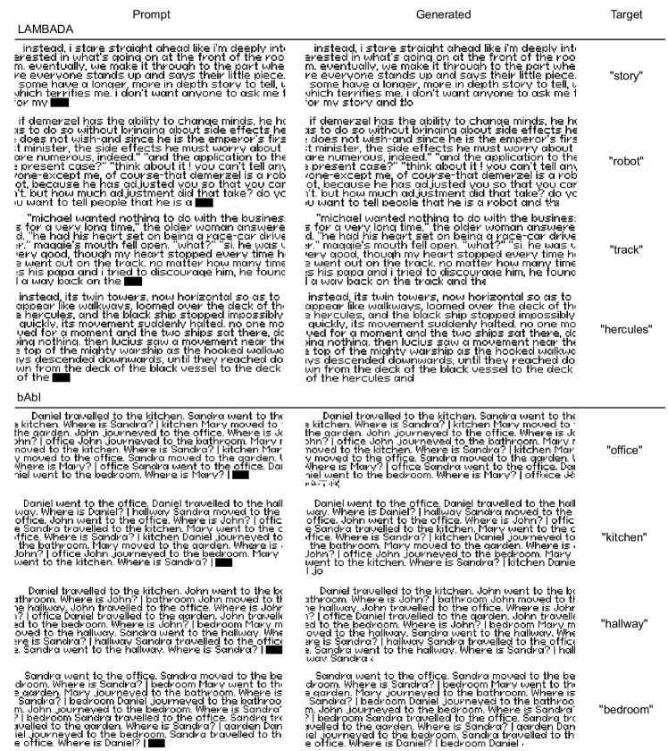
Figure 5: Pixar generation samples from LAMBADA and bAbI dataset. Images are folded into rectangles for better readability.

References

- Aghajanyan et al. (2022) Aghajanyan, A., Huang, B., Ross, C., Karpukhin, V., Xu, H., Goyal, N., Okhonko, D., Joshi, M., Ghosh, G., Lewis, M., and Zettlemoyer, L. Cm3: A causal masked multimodal model of the internet, 2022.
- Aghajanyan et al. (2023) Aghajanyan, A., Yu, L., Conneau, A., Hsu, W.-N., Hambardzumyan, K., Zhang, S., Roller, S., Goyal, N., Levy, O., and Zettlemoyer, L. Scaling laws for generative mixed-modal language models, 2023.
- Bao et al. (2022) Bao, H., Dong, L., Piao, S., and Wei, F. Beit: Bert pre-training of image transformers, 2022.
- Bird et al. (2009) Bird, S., Klein, E., and Loper, E. Natural language processing with Python: analyzing text with the natural language toolkit. ” O’Reilly Media, Inc.”, 2009.
- Brown et al. (2020) Brown, T. B., Mann, B., Ryder, N., Subbiah, M., Kaplan, J., Dhariwal, P., Neelakantan, A., Shyam, P., Sastry, G., Askell, A., Agarwal, S., Herbert-Voss, A., Krueger, G., Henighan, T., Child, R., Ramesh, A., Ziegler, D. M., Wu, J., Winter, C., Hesse, C., Chen, M., Sigler, E., Litwin, M., Gray, S., Chess, B., Clark, J., Berner, C., McCandlish, S., Radford, A., Sutskever, I., and Amodei, D. Language models are few-shot learners, 2020.
- Chang et al. (2022) Chang, H., Zhang, H., Jiang, L., Liu, C., and Freeman, W. T. Maskgit: Masked generative image transformer, 2022.
- Chang et al. (2023) Chang, H., Zhang, H., Barber, J., Maschinot, A., Lezama, J., Jiang, L., Yang, M.-H., Murphy, K., Freeman, W. T., Rubinstein, M., Li, Y., and Krishnan, D. Muse: Text-to-image generation via masked generative transformers, 2023.
- Chen et al. (2020a) Chen, M., Radford, A., Child, R., Wu, J., Jun, H., Luan, D., and Sutskever, I. Generative pretraining from pixels. In International conference on machine learning, pp. 1691–1703. PMLR, 2020a.
- Chen et al. (2020b) Chen, M., Radford, A., Child, R., Wu, J., Jun, H., Luan, D., and Sutskever, I. Generative pretraining from pixels. In International conference on machine learning, pp. 1691–1703. PMLR, 2020b.
- Cui et al. (2020) Cui, Y., Che, W., Liu, T., Qin, B., Wang, S., and Hu, G. Revisiting pre-trained models for chinese natural language processing. In Findings of the Association for Computational Linguistics: EMNLP 2020. Association for Computational Linguistics, 2020. doi: 10.18653/v1/2020.findings-emnlp.58. URL http://dx.doi.org/10.18653/v1/2020.findings-emnlp.58.
- Dai & Cai (2017) Dai, F. and Cai, Z. Glyph-aware embedding of Chinese characters. In Faruqui, M., Schuetze, H., Trancoso, I., and Yaghoobzadeh, Y. (eds.), Proceedings of the First Workshop on Subword and Character Level Models in NLP, pp. 64–69, Copenhagen, Denmark, September 2017. Association for Computational Linguistics. doi: 10.18653/v1/W17-4109. URL https://aclanthology.org/W17-4109.
- Devlin et al. (2019) Devlin, J., Chang, M.-W., Lee, K., and Toutanova, K. Bert: Pre-training of deep bidirectional transformers for language understanding, 2019.
- Eger et al. (2020) Eger, S., Şahin, G. G., Rücklé, A., Lee, J.-U., Schulz, C., Mesgar, M., Swarnkar, K., Simpson, E., and Gurevych, I. Text processing like humans do: Visually attacking and shielding nlp systems, 2020.
- Esser et al. (2021) Esser, P., Rombach, R., and Ommer, B. Taming transformers for high-resolution image synthesis, 2021.
- Goodfellow et al. (2014) Goodfellow, I. J., Pouget-Abadie, J., Mirza, M., Xu, B., Warde-Farley, D., Ozair, S., Courville, A., and Bengio, Y. Generative adversarial networks, 2014.
- He et al. (2021) He, K., Chen, X., Xie, S., Li, Y., Dollár, P., and Girshick, R. Masked autoencoders are scalable vision learners, 2021.
- Jaegle et al. (2021) Jaegle, A., Gimeno, F., Brock, A., Zisserman, A., Vinyals, O., and Carreira, J. Perceiver: General perception with iterative attention, 2021.
- Jozefowicz et al. (2016) Jozefowicz, R., Vinyals, O., Schuster, M., Shazeer, N., and Wu, Y. Exploring the limits of language modeling, 2016.
- Kaddour et al. (2023) Kaddour, J., Harris, J., Mozes, M., Bradley, H., Raileanu, R., and McHardy, R. Challenges and applications of large language models, 2023.
- Kudo & Richardson (2018) Kudo, T. and Richardson, J. Sentencepiece: A simple and language independent subword tokenizer and detokenizer for neural text processing, 2018.
- Li et al. (2023a) Li, J., Zhao, W. X., Nie, J.-Y., and Wen, J.-R. Glyphdiffusion: Text generation as image generation, 2023a.
- Li et al. (2023b) Li, T., Chang, H., Mishra, S. K., Zhang, H., Katabi, D., and Krishnan, D. Mage: Masked generative encoder to unify representation learning and image synthesis, 2023b.
- Liu et al. (2017) Liu, F., Lu, H., Lo, C., and Neubig, G. Learning character-level compositionality with visual features. In Barzilay, R. and Kan, M.-Y. (eds.), Proceedings of the 55th Annual Meeting of the Association for Computational Linguistics (Volume 1: Long Papers), pp. 2059–2068, Vancouver, Canada, July 2017. Association for Computational Linguistics. doi: 10.18653/v1/P17-1188. URL https://aclanthology.org/P17-1188.
- Liu et al. (2021) Liu, F., Bugliarello, E., Ponti, E. M., Reddy, S., Collier, N., and Elliott, D. Visually grounded reasoning across languages and cultures. In Proceedings of the 2021 Conference on Empirical Methods in Natural Language Processing, pp. 10467–10485, Online and Punta Cana, Dominican Republic, November 2021. Association for Computational Linguistics. URL https://aclanthology.org/2021.emnlp-main.818.
- Loshchilov & Hutter (2017) Loshchilov, I. and Hutter, F. Sgdr: Stochastic gradient descent with warm restarts, 2017.
- Loshchilov & Hutter (2019) Loshchilov, I. and Hutter, F. Decoupled weight decay regularization, 2019.
- Meng et al. (2020) Meng, Y., Wu, W., Wang, F., Li, X., Nie, P., Yin, F., Li, M., Han, Q., Sun, X., and Li, J. Glyce: Glyph-vectors for chinese character representations, 2020.
- Menick & Kalchbrenner (2018) Menick, J. and Kalchbrenner, N. Generating high fidelity images with subscale pixel networks and multidimensional upscaling, 2018.
- Osborne & Rubinstein (1994) Osborne, M. J. and Rubinstein, A. A Course in Game Theory. The MIT Press, 1994. ISBN 0262150417.
- Paperno et al. (2016) Paperno, D., Kruszewski, G., Lazaridou, A., Pham, Q. N., Bernardi, R., Pezzelle, S., Baroni, M., Boleda, G., and Fernández, R. The lambada dataset: Word prediction requiring a broad discourse context, 2016.
- Penedo et al. (2023) Penedo, G., Malartic, Q., Hesslow, D., Cojocaru, R., Cappelli, A., Alobeidli, H., Pannier, B., Almazrouei, E., and Launay, J. The refinedweb dataset for falcon llm: Outperforming curated corpora with web data, and web data only, 2023.
- Radford et al. (2019) Radford, A., Wu, J., Child, R., Luan, D., Amodei, D., and Sutskever, I. Language models are unsupervised multitask learners. 2019.
- Ramesh et al. (2022) Ramesh, A., Dhariwal, P., Nichol, A., Chu, C., and Chen, M. Hierarchical text-conditional image generation with clip latents, 2022.
- Rombach et al. (2022) Rombach, R., Blattmann, A., Lorenz, D., Esser, P., and Ommer, B. High-resolution image synthesis with latent diffusion models, 2022.
- Rust et al. (2023) Rust, P., Lotz, J. F., Bugliarello, E., Salesky, E., de Lhoneux, M., and Elliott, D. Language modelling with pixels, 2023.
- Salesky et al. (2021) Salesky, E., Etter, D., and Post, M. Robust open-vocabulary translation from visual text representations, 2021.
- Salesky et al. (2023) Salesky, E., Verma, N., Koehn, P., and Post, M. Multilingual pixel representations for translation and effective cross-lingual transfer, 2023.
- Salimans et al. (2017) Salimans, T., Karpathy, A., Chen, X., and Kingma, D. P. Pixelcnn++: Improving the pixelcnn with discretized logistic mixture likelihood and other modifications, 2017.
- Sennrich et al. (2016) Sennrich, R., Haddow, B., and Birch, A. Neural machine translation of rare words with subword units, 2016.
- Shannon (1948) Shannon, C. E. A mathematical theory of communication. The Bell system technical journal, 27(3):379–423, 1948.
- Shazeer (2020) Shazeer, N. Glu variants improve transformer, 2020.
- Su et al. (2023) Su, J., Lu, Y., Pan, S., Murtadha, A., Wen, B., and Liu, Y. Roformer: Enhanced transformer with rotary position embedding, 2023.
- Sun et al. (2018) Sun, B., Yang, L., Dong, P., Zhang, W., Dong, J., and Young, C. Super characters: A conversion from sentiment classification to image classification. In Proceedings of the 9th Workshop on Computational Approaches to Subjectivity, Sentiment and Social Media Analysis, pp. 309–315, Brussels, Belgium, October 2018. Association for Computational Linguistics. doi: 10.18653/v1/W18-6245. URL https://aclanthology.org/W18-6245.
- Sun et al. (2021) Sun, Z., Li, X., Sun, X., Meng, Y., Ao, X., He, Q., Wu, F., and Li, J. ChineseBERT: Chinese pretraining enhanced by glyph and Pinyin information. In Proceedings of the 59th Annual Meeting of the Association for Computational Linguistics and the 11th International Joint Conference on Natural Language Processing (Volume 1: Long Papers), pp. 2065–2075, Online, August 2021. Association for Computational Linguistics. doi: 10.18653/v1/2021.acl-long.161. URL https://aclanthology.org/2021.acl-long.161.
- Touvron et al. (2023a) Touvron, H., Lavril, T., Izacard, G., Martinet, X., Lachaux, M.-A., Lacroix, T., Rozière, B., Goyal, N., Hambro, E., Azhar, F., Rodriguez, A., Joulin, A., Grave, E., and Lample, G. Llama: Open and efficient foundation language models, 2023a.
- Touvron et al. (2023b) Touvron, H., Martin, L., Stone, K., Albert, P., Almahairi, A., Babaei, Y., Bashlykov, N., Batra, S., Bhargava, P., Bhosale, S., Bikel, D., Blecher, L., Ferrer, C. C., Chen, M., Cucurull, G., Esiobu, D., Fernandes, J., Fu, J., Fu, W., Fuller, B., Gao, C., Goswami, V., Goyal, N., Hartshorn, A., Hosseini, S., Hou, R., Inan, H., Kardas, M., Kerkez, V., Khabsa, M., Kloumann, I., Korenev, A., Koura, P. S., Lachaux, M.-A., Lavril, T., Lee, J., Liskovich, D., Lu, Y., Mao, Y., Martinet, X., Mihaylov, T., Mishra, P., Molybog, I., Nie, Y., Poulton, A., Reizenstein, J., Rungta, R., Saladi, K., Schelten, A., Silva, R., Smith, E. M., Subramanian, R., Tan, X. E., Tang, B., Taylor, R., Williams, A., Kuan, J. X., Xu, P., Yan, Z., Zarov, I., Zhang, Y., Fan, A., Kambadur, M., Narang, S., Rodriguez, A., Stojnic, R., Edunov, S., and Scialom, T. Llama 2: Open foundation and fine-tuned chat models, 2023b.
- Tschannen et al. (2023) Tschannen, M., Eastwood, C., and Mentzer, F. Givt: Generative infinite-vocabulary transformers, 2023.
- van den Oord et al. (2016) van den Oord, A., Kalchbrenner, N., and Kavukcuoglu, K. Pixel recurrent neural networks, 2016.
- van den Oord et al. (2018) van den Oord, A., Vinyals, O., and Kavukcuoglu, K. Neural discrete representation learning, 2018.
- Vaswani et al. (2023) Vaswani, A., Shazeer, N., Parmar, N., Uszkoreit, J., Jones, L., Gomez, A. N., Kaiser, L., and Polosukhin, I. Attention is all you need, 2023.
- Wang et al. (2018) Wang, A., Singh, A., Michael, J., Hill, F., Levy, O., and Bowman, S. GLUE: A multi-task benchmark and analysis platform for natural language understanding. In Linzen, T., Chrupała, G., and Alishahi, A. (eds.), Proceedings of the 2018 EMNLP Workshop BlackboxNLP: Analyzing and Interpreting Neural Networks for NLP, pp. 353–355, Brussels, Belgium, November 2018. Association for Computational Linguistics. doi: 10.18653/v1/W18-5446. URL https://aclanthology.org/W18-5446.
- Weston et al. (2015) Weston, J., Bordes, A., Chopra, S., Rush, A. M., van Merriënboer, B., Joulin, A., and Mikolov, T. Towards ai-complete question answering: A set of prerequisite toy tasks, 2015.
- Workshop et al. (2023) Workshop, B., :, Scao, T. L., Fan, A., Akiki, C., Pavlick, E., Ilić, S., Hesslow, D., Castagné, R., Luccioni, A. S., Yvon, F., Gallé, M., Tow, J., Rush, A. M., Biderman, S., Webson, A., Ammanamanchi, P. S., Wang, T., Sagot, B., Muennighoff, N., del Moral, A. V., Ruwase, O., Bawden, R., Bekman, S., McMillan-Major, A., Beltagy, I., Nguyen, H., Saulnier, L., Tan, S., Suarez, P. O., Sanh, V., Laurençon, H., Jernite, Y., Launay, J., Mitchell, M., Raffel, C., Gokaslan, A., Simhi, A., Soroa, A., Aji, A. F., Alfassy, A., Rogers, A., Nitzav, A. K., Xu, C., Mou, C., Emezue, C., Klamm, C., Leong, C., van Strien, D., Adelani, D. I., Radev, D., Ponferrada, E. G., Levkovizh, E., Kim, E., Natan, E. B., Toni, F. D., Dupont, G., Kruszewski, G., Pistilli, G., Elsahar, H., Benyamina, H., Tran, H., Yu, I., Abdulmumin, I., Johnson, I., Gonzalez-Dios, I., de la Rosa, J., Chim, J., Dodge, J., Zhu, J., Chang, J., Frohberg, J., Tobing, J., Bhattacharjee, J., Almubarak, K., Chen, K., Lo, K., Werra, L. V., Weber, L., Phan, L., allal, L. B., Tanguy, L., Dey, M., Muñoz, M. R., Masoud, M., Grandury, M., Šaško, M., Huang, M., Coavoux, M., Singh, M., Jiang, M. T.-J., Vu, M. C., Jauhar, M. A., Ghaleb, M., Subramani, N., Kassner, N., Khamis, N., Nguyen, O., Espejel, O., de Gibert, O., Villegas, P., Henderson, P., Colombo, P., Amuok, P., Lhoest, Q., Harliman, R., Bommasani, R., López, R. L., Ribeiro, R., Osei, S., Pyysalo, S., Nagel, S., Bose, S., Muhammad, S. H., Sharma, S., Longpre, S., Nikpoor, S., Silberberg, S., Pai, S., Zink, S., Torrent, T. T., Schick, T., Thrush, T., Danchev, V., Nikoulina, V., Laippala, V., Lepercq, V., Prabhu, V., Alyafeai, Z., Talat, Z., Raja, A., Heinzerling, B., Si, C., Taşar, D. E., Salesky, E., Mielke, S. J., Lee, W. Y., Sharma, A., Santilli, A., Chaffin, A., Stiegler, A., Datta, D., Szczechla, E., Chhablani, G., Wang, H., Pandey, H., Strobelt, H., Fries, J. A., Rozen, J., Gao, L., Sutawika, L., Bari, M. S., Al-shaibani, M. S., Manica, M., Nayak, N., Teehan, R., Albanie, S., Shen, S., Ben-David, S., Bach, S. H., Kim, T., Bers, T., Fevry, T., Neeraj, T., Thakker, U., Raunak, V., Tang, X., Yong, Z.-X., Sun, Z., Brody, S., Uri, Y., Tojarieh, H., Roberts, A., Chung, H. W., Tae, J., Phang, J., Press, O., Li, C., Narayanan, D., Bourfoune, H., Casper, J., Rasley, J., Ryabinin, M., Mishra, M., Zhang, M., Shoeybi, M., Peyrounette, M., Patry, N., Tazi, N., Sanseviero, O., von Platen, P., Cornette, P., Lavallée, P. F., Lacroix, R., Rajbhandari, S., Gandhi, S., Smith, S., Requena, S., Patil, S., Dettmers, T., Baruwa, A., Singh, A., Cheveleva, A., Ligozat, A.-L., Subramonian, A., Névéol, A., Lovering, C., Garrette, D., Tunuguntla, D., Reiter, E., Taktasheva, E., Voloshina, E., Bogdanov, E., Winata, G. I., Schoelkopf, H., Kalo, J.-C., Novikova, J., Forde, J. Z., Clive, J., Kasai, J., Kawamura, K., Hazan, L., Carpuat, M., Clinciu, M., Kim, N., Cheng, N., Serikov, O., Antverg, O., van der Wal, O., Zhang, R., Zhang, R., Gehrmann, S., Mirkin, S., Pais, S., Shavrina, T., Scialom, T., Yun, T., Limisiewicz, T., Rieser, V., Protasov, V., Mikhailov, V., Pruksachatkun, Y., Belinkov, Y., Bamberger, Z., Kasner, Z., Rueda, A., Pestana, A., Feizpour, A., Khan, A., Faranak, A., Santos, A., Hevia, A., Unldreaj, A., Aghagol, A., Abdollahi, A., Tammour, A., HajiHosseini, A., Behroozi, B., Ajibade, B., Saxena, B., Ferrandis, C. M., McDuff, D., Contractor, D., Lansky, D., David, D., Kiela, D., Nguyen, D. A., Tan, E., Baylor, E., Ozoani, E., Mirza, F., Ononiwu, F., Rezanejad, H., Jones, H., Bhattacharya, I., Solaiman, I., Sedenko, I., Nejadgholi, I., Passmore, J., Seltzer, J., Sanz, J. B., Dutra, L., Samagaio, M., Elbadri, M., Mieskes, M., Gerchick, M., Akinlolu, M., McKenna, M., Qiu, M., Ghauri, M., Burynok, M., Abrar, N., Rajani, N., Elkott, N., Fahmy, N., Samuel, O., An, R., Kromann, R., Hao, R., Alizadeh, S., Shubber, S., Wang, S., Roy, S., Viguier, S., Le, T., Oyebade, T., Le, T., Yang, Y., Nguyen, Z., Kashyap, A. R., Palasciano, A., Callahan, A., Shukla, A., Miranda-Escalada, A., Singh, A., Beilharz, B., Wang, B., Brito, C., Zhou, C., Jain, C., Xu, C., Fourrier, C., Periñán, D. L., Molano, D., Yu, D., Manjavacas, E., Barth, F., Fuhrimann, F., Altay, G., Bayrak, G., Burns, G., Vrabec, H. U., Bello, I., Dash, I., Kang, J., Giorgi, J., Golde, J., Posada, J. D., Sivaraman, K. R., Bulchandani, L., Liu, L., Shinzato, L., de Bykhovetz, M. H., Takeuchi, M., Pàmies, M., Castillo, M. A., Nezhurina, M., Sänger, M., Samwald, M., Cullan, M., Weinberg, M., Wolf, M. D., Mihaljcic, M., Liu, M., Freidank, M., Kang, M., Seelam, N., Dahlberg, N., Broad, N. M., Muellner, N., Fung, P., Haller, P., Chandrasekhar, R., Eisenberg, R., Martin, R., Canalli, R., Su, R., Su, R., Cahyawijaya, S., Garda, S., Deshmukh, S. S., Mishra, S., Kiblawi, S., Ott, S., Sang-aroonsiri, S., Kumar, S., Schweter, S., Bharati, S., Laud, T., Gigant, T., Kainuma, T., Kusa, W., Labrak, Y., Bajaj, Y. S., Venkatraman, Y., Xu, Y., Xu, Y., Xu, Y., Tan, Z., Xie, Z., Ye, Z., Bras, M., Belkada, Y., and Wolf, T. Bloom: A 176b-parameter open-access multilingual language model, 2023.
- Wu et al. (2016) Wu, Y., Schuster, M., Chen, Z., Le, Q. V., Norouzi, M., Macherey, W., Krikun, M., Cao, Y., Gao, Q., Macherey, K., Klingner, J., Shah, A., Johnson, M., Liu, X., Łukasz Kaiser, Gouws, S., Kato, Y., Kudo, T., Kazawa, H., Stevens, K., Kurian, G., Patil, N., Wang, W., Young, C., Smith, J., Riesa, J., Rudnick, A., Vinyals, O., Corrado, G., Hughes, M., and Dean, J. Google’s neural machine translation system: Bridging the gap between human and machine translation, 2016.
- Xue et al. (2021) Xue, L., Constant, N., Roberts, A., Kale, M., Al-Rfou, R., Siddhant, A., Barua, A., and Raffel, C. mt5: A massively multilingual pre-trained text-to-text transformer, 2021.