Data-Dependent Stability Analysis of Adversarial Training

Yihan Wang1,2, Shuang Liu1,2, Xiao-Shan Gao1,2 Corresponding author.
Abstract

Stability analysis is an essential aspect of studying the generalization ability of deep learning, as it involves deriving generalization bounds for stochastic gradient descent-based training algorithms. Adversarial training is the most widely used defense against adversarial example attacks. However, previous generalization bounds for adversarial training have not included information regarding the data distribution. In this paper, we fill this gap by providing generalization bounds for stochastic gradient descent-based adversarial training that incorporate data distribution information. We utilize the concepts of on-average stability and high-order approximate Lipschitz conditions to examine how changes in data distribution and adversarial budget can affect robust generalization gaps. Our derived generalization bounds for both convex and non-convex losses are at least as good as the uniform stability-based counterparts which do not include data distribution information. Furthermore, our findings demonstrate how distribution shifts from data poisoning attacks can impact robust generalization.

1 Introduction

Deep learning models acquire knowledge from training data and generalize to unseen data. Generalization plays a key role in successful machine learning algorithms. On the other hand, a neural network can be easily fooled by adversarial examples (Szegedy etΒ al. 2013; Goodfellow, Shlens, and Szegedy 2014). Though adversarial training (Madry etΒ al. 2017) can largely alleviate the adversarial vulnerability of networks, the corresponding robust generalization is more difficult and robust overfitting (Rice, Wong, and Kolter 2020) harms the robust performance to a very large degree. To understand the generalization ability of adversarial training, an important research direction is to give a theoretical analysis of its generalization bounds.

Algorithmic stability (Bousquet and Elisseeff 2002; Shalev-Shwartz etΒ al. 2010) can derive the generalization bounds. In standard training, the uniform stability of stochastic gradient descent (SGD) was studied by Hardt, Recht, and Singer (2016), assuming the loss function is $L$-Lipschitz and $\beta$-gradient Lipschitz. Bassily etΒ al. (2020) extended the results to non-smooth convex losses. Kuzborskij and Lampert (2018) employed on-average stability and provided data-dependent generalization bounds. In adversarial training, the stability of minimax problems is discussed by Farnia and Ozdaglar (2021), assuming the inner maximization problem is strongly concave. Xing, Song, and Cheng (2021) considered the uniform stability of adversarial training on non-smooth losses. Under the $\eta$-approximate $\beta$-gradient Lipschitz assumption, Xiao etΒ al. (2022) derived generalization bounds for SGD in adversarial training, which involved the adversarial training budget.

It is generally believed that the difficulty of robust generalization involves three aspects including model capacity, training algorithm, and data distribution. The capacity of a strictly robust classifier on a well-separated distribution should be exponential in the data dimension (Li etΒ al. 2022). The previous generalization bounds based on uniform stability analyses (Xing, Song, and Cheng 2021; Xiao etΒ al. 2022) of adversarial training algorithms did not contain information about data distribution.

In this paper, we analyze the on-average stability of SGD-based adversarial training and derive data-dependent generalization bounds to illustrate robust generalization, that is, the generalization bounds contain information of data distribution. For the convex adversarial losses, assuming the losses are Lipschitz and approximately gradient Lipschitz, we give a generalization bound dependent on the adversarial population risk at the initialization point and the variance of stochastic gradients over the distribution. Assuming the losses are approximately Hessian Lipschitz in addition, we provide a generalization bound for the non-convex adversarial losses. Besides the variance of stochastic gradients over the distribution, this bound depends on the curvature (the norm of the Hessian matrix) at the initialization point and the population risk at the output parameters. Our bounds grow with the adversarial training budget and cover the standard training setting when the budget becomes zero. Our bounds for both convex and non-convex losses are no worse than the uniform stability-based counterparts but capture the information about the data distribution and the initialization point.

An additional advantage of our generalization bound over the previous ones is that it describes the effects of distribution shifts caused by data poisoning attacks and hence interprets the shrinkage of generalization gaps in adversarial training under stability attacks since the poisoned distributions can reduce the adversarial population risk over the poisoned data.

The rest of the paper is organized as follows. In Section 3, we revisit the relationship between stability and robust generalization for adversarial training. In Section 4, we provide our main results. In Section 5, we present experimental results to verify the theoretical results. All proofs are deferred to Appendix A.

2 Related Works

Robust Generalization. Machine learning models are highly vulnerable to adversarial examples (Szegedy etΒ al. 2013; Biggio etΒ al. 2013; Nguyen, Yosinski, and Clune 2015; Moosavi-Dezfooli, Fawzi, and Frossard 2016), where crafted and imperceptible perturbations to input data can easily fool a well-trained classifier. A widely adopted illustration attributes adversarial examples to the presence of non-robust features (Ilyas etΒ al. 2019). Among numerous proposed defenses against adversarial attacks, adversarial training (Goodfellow, Shlens, and Szegedy 2014; Shaham, Yamada, and Negahban 2015; Madry etΒ al. 2017) has become a major approach to training a robust deep neural network and can achieve optimal robust accuracy if certain loss functions are used (Gao, Liu, and Yu 2022).

The generalization in adversarial training is much more tricky than that in standard training and requires more data and larger models (Schmidt etΒ al. 2018; Gowal etΒ al. 2021; Li etΒ al. 2022; Wang etΒ al. 2023). The robust overfitting (Rice, Wong, and Kolter 2020) phenomenon harms the robustness in a long training procedure. In recent years, different methods (Chen etΒ al. 2020; Wu, Xia, and Wang 2020; Yu etΒ al. 2022a; Chen etΒ al. 2022) have been proposed to alleviate robust overfitting.

Algorithmic Stability. Modern stability analysis goes back to the work of Bousquet and Elisseeff (2002). Notions of stability fall into two categories: data-free and data-dependent ones. The first category is usually called uniform stability. Generalization bounds of SGD have been analyzed using uniform stability under Lipschitz and smoothness conditions by Hardt, Recht, and Singer (2016). Bassily etΒ al. (2020) extended the results to the non-smooth convex case. Farnia and Ozdaglar (2021) studied the role of optimization algorithm in the generalization performance of the minimax model. The uniform stability of adversarial training has been reported by Xing, Song, and Cheng (2021); Xiao etΒ al. (2022). The data-dependent stability (Kuzborskij and Lampert 2018) employing the notion of on-average stability (Shalev-Shwartz etΒ al. 2010) focused on the stability of the SGD-based standard training under the data distribution given an initialization point.

Data Poisoning. As defensive strategies against unauthorized exploitation of personal data, availability attacks (Huang etΒ al. 2021; Fowl etΒ al. 2021; Feng, Cai, and Zhou 2019; Liu etΒ al. 2021; Ren etΒ al. 2022) perturb the training data imperceptibly such that the trained models learn nothing useful and become futile. Adversarial training can mitigate such availability attacks (Tao etΒ al. 2021). Stability attacks (Tao etΒ al. 2022; Fu etΒ al. 2022; Wang, Wang, and Wang 2021) have been proposed to come through adversarial training and result in a large degradation in the robust test performance. The shortcut interpretation (Yu etΒ al. 2022b) suggests that stability poisoning attacks root ”easy-to-learn” features in the poisoned training data. However, these features do not appear in clean data. Our generalization bound can be used to interpret the shrinkage of generalization gaps in adversarial training under stability attacks, since it contains information of data distribution.

3 Preliminaries

In this section, we revisit the robust generalization gap and the on-average stability analysis.

3.1 Robust Generalization Gap

Let ${\mathcal{D}}$ be a data distribution over an image classification data space ${\mathbb{D}}=[0,1]^{d}\times[m]$, where $[0,1]^{d}$ contains the image space and $[m]=\{1,\ldots,m\}$ is the label set. A data set $S$ of $n$ samples is drawn i.i.d. from ${\mathcal{D}}$ and is denoted by $S\sim{\mathcal{D}}^{n}$. Given a network with parameter $\theta$ and a non-negative loss function $l(\theta,z):{\mathbb{R}}^{k}\times{\mathbb{D}}\to{\mathbb{R}}_{\geq 0}$, the standard training minimizes the empirical risk $\mathop{\mathbb{E}}_{z\in S}\,l(\theta,z)$ with SGD.

Adversarial Training. As a major defense approach, adversarial training (Madry etΒ al. 2017) refers to a bi-level optimization, of which the inner maximization iteratively searches for the strongest perturbation inside a $L_{p}$-norm ball and the outer minimization optimizes the model via the loss on the perturbed data. Formally, given an adversarial budget $\epsilon$, the adversarial training uses the adversarial loss:

$\displaystyle h(\theta,z)=\max_{z^{\prime}\in{\mathcal{B}}_{\epsilon}(z)}l(z^{\prime},\theta),$

where ${\mathcal{B}}_{\epsilon}(z)=\{z^{\prime}\in{\mathbb{D}}:||z^{\prime}-z||_{p}\leq\epsilon\}$ and $p\in{\mathbb{N}}\cup\{\infty\}$. Here the $p$-norm is for the image part of $z$. When $\epsilon=0$, we have $h=l$ and adversarial training reduces to standard training. The adversarial population risk and adversarial empirical risk are respectively defined as

$\displaystyle{\mathcal{R}}_{\mathcal{D}}(\theta)=\mathop{\mathbb{E}}_{z\sim{\mathcal{D}}}[h(\theta,z)]\text{\ \ \ and\ \ \ }{\mathcal{R}}_{S}(\theta)=\mathop{\mathbb{E}}_{z\in S}[h(\theta,z)].$

We denote the SGD algorithm of adversarial training by ${\mathcal{A}}$, which inputs a training set $S$ and outputs the parameter ${\mathcal{A}}(S)$ of a network through minimizing the adversarial empirical risk ${\mathcal{R}}_{S}$.

Robust Generalization Gap. Let $\theta^{*},\bar{\theta}$ be the optimal solutions of learning over ${\mathcal{D}}$ and $S$, namely minimizing ${\mathcal{R}}_{\mathcal{D}}(\theta)$ and ${\mathcal{R}}_{S}(\theta)$, respectively. Then, for the output $\hat{\theta}={\mathcal{A}}(S)$ of algorithm ${\mathcal{A}}$, the excess risk can be decomposed as

$\displaystyle{\mathcal{R}}_{\mathcal{D}}(\hat{\theta})-{\mathcal{R}}_{\mathcal{D}}(\theta^{*})$ $\displaystyle=\underbrace{{\mathcal{R}}_{\mathcal{D}}(\hat{\theta})-{\mathcal{R}}_{S}(\hat{\theta})}_{\varepsilon_{\hbox{\rm{gen}}}}+\underbrace{{\mathcal{R}}_{S}(\hat{\theta})-{\mathcal{R}}_{S}(\bar{\theta})}_{\varepsilon_{\hbox{\rm{opt}}}}$
$\displaystyle+$ $\displaystyle\underbrace{{\mathcal{R}}_{S}(\bar{\theta})-{\mathcal{R}}_{S}(\theta^{*})}_{\leq 0}+\underbrace{{\mathcal{R}}_{S}(\theta^{*})-{\mathcal{R}}_{\mathcal{D}}(\theta^{*})}_{\mathop{\mathbb{E}}=0}.$

To control the excess risk, we need to control the robust generalization gap $\varepsilon_{\hbox{\rm{gen}}}$ and the robust optimization gap $\varepsilon_{\hbox{\rm{opt}}}$. The robust optimization gap in adversarial training has been studied a lot theoretically (Nemirovski etΒ al. 2009; Xiao etΒ al. 2022). Also, empirical results (Madry etΒ al. 2017; Zhang etΒ al. 2019; Wang etΒ al. 2019; Wu, Xia, and Wang 2020) present narrow robust optimization gaps.

On the other hand, robust overfitting (Rice, Wong, and Kolter 2020) is a dominant phenomenon in adversarial training that hinders deep neural networks from attaining high robust performance. Hence, we focus on the robust generalization gap $\varepsilon_{\hbox{\rm{gen}}}$ in this paper.

3.2 On-Average Stability

In order to analyze the data-dependent stability, we employ the notion of on-average stability. Given a data set $S=\{z_{1},\cdots,z_{n}\}\sim{\mathcal{D}}^{n}$ and $z\sim{\mathcal{D}}$, replacing $z_{i}$ in $S$ with $z$, we denote $S^{i,z}=\{z_{1},\cdots,z_{i-1},z,z_{i+1},\cdots,z_{n}\}$ with $i\in[n]$.

Definition 1 (On-Average Stability).

A randomized algorithm ${\mathcal{A}}$ is $\varepsilon$-on-average stable if

$\displaystyle\sup_{i\in[n]}\mathop{\mathbb{E}}_{S,z,{\mathcal{A}}}[h({\mathcal{A}}(S),z)-h({\mathcal{A}}(S^{i,z}),z)]\leq\varepsilon,$ (1)

where $S\sim{\mathcal{D}}^{n}$, $z\sim{\mathcal{D}}$, and $\varepsilon$ can depend on the data distribution ${\mathcal{D}}$ and the initialization point of ${\mathcal{A}}$.

The on-average stability considers the expected difference between the losses of algorithm outputs on $S$ and its replace-one-example version for all replacement index $i$. The on-average stability derives the upper bound of the generalization gap as follows.

Theorem 2 (Kuzborskij and Lampert (2018)).

If ${\mathcal{A}}$ is $\varepsilon$-on-average stable, then the robust generalization gap of ${\mathcal{A}}$ is bounded by $\varepsilon$:

$\displaystyle\mathop{\mathbb{E}}_{S,{\mathcal{A}}}[{\mathcal{R}}_{\mathcal{D}}({\mathcal{A}}(S))-{\mathcal{R}}_{S}({\mathcal{A}}(S))]\leq\varepsilon.$

4 Theoretical Results

In this section, we give the data-dependent stability analysis of adversarial training for both convex and non-convex adversarial losses. We provide proof sketches of our results and the full proofs are placed in Appendix A.

4.1 Lipschitz Conditions

Stability analysis always relies on some Lipschitz conditions. The loss function is assumed to be $L$-Lipschitz and $\beta$-gradient Lipschitz, i.e. $\beta$-smooth in the work (Hardt, Recht, and Singer 2016). For adversarial training, we need the adversarial loss $h(\theta,z)$ to satisfy some Lipschitz conditions. It is not reasonable to directly endow $h$ with Lipschitz conditions, since $h(\theta,z)$ takes the maximum of $l(\theta,z^{\prime})$ with $z^{\prime}\in{\mathcal{B}}_{\epsilon}(z)$. Instead, we assume that the original loss function $l(\theta,z)$ satisfies the following Lipschitz conditions. Let $||\cdot||_{p}$ be the $p$-norm of vectors or matrices and we write $||\cdot||$ instead of $||\cdot||_{2}$ for brevity. In this paper, $\nabla$ is the abbreviation for $\nabla_{\theta}$.

Assumption 3.

The loss $l$ is $L$-Lipschitz in $\theta$:

$\displaystyle||l(\theta_{1},z)-l(\theta_{2},z)||$ $\displaystyle\leq L||\theta_{1}-\theta_{2}||.$
Assumption 4.

The loss $l$ is $L_{\theta}$-gradient Lipschitz in $\theta$ and $L_{z}$-gradient Lipschitz in $z$:

$\displaystyle||\nabla l(\theta_{1},z)-\nabla l(\theta_{2},z)||$ $\displaystyle\leq L_{\theta}||\theta_{1}-\theta_{2}||,$
$\displaystyle||\nabla l(\theta,z_{1})-\nabla l(\theta,z_{2})||$ $\displaystyle\leq L_{z}||z_{1}-z_{2}||_{p}.$
Assumption 5.

The loss $l$ is $H_{\theta}$-Hessian Lipschitz in $\theta$ and $H_{z}$-Hessian Lipschitz in $z$:

$\displaystyle||\nabla^{2}l(\theta_{1},z)-\nabla^{2}l(\theta_{2},z)||$ $\displaystyle\leq H_{\theta}||\theta_{1}-\theta_{2}||,$
$\displaystyle||\nabla^{2}l(\theta,z_{1})-\nabla^{2}l(\theta,z_{2})||$ $\displaystyle\leq H_{z}||z_{1}-z_{2}||_{p}.$
Remark 6.

For commonly used losses and ReLU-based networks, Assumption 3 is valid (Gao, Liu, and Yu 2022). The gradient Lipschitz conditions (Lipschitz smoothness) are often used in robustness analysis (Sinha etΒ al. 2017; Liu etΒ al. 2020; Xiao etΒ al. 2022). Lipschitz Hessians are used in the analysis of SGD (Ge etΒ al. 2015; Kuzborskij and Lampert 2018). Assumptions 4 and 5 are valid for networks based on smooth activation functions such as Sigmoid and smooth loss functions such as cross-entropy (CE) and mean squared error (MSE); related works on ReLU-based networks were given in (Allen-Zhu, Li, and Song 2019; Du etΒ al. 2019).

Note that the adversarial vulnerability of deep networks is rooted in the explosion of the Lipschitz constant of $l(\theta,z)$ in $z$. However, the zero-order Lipschitz constant in $\theta$ can be directly inherited by $h(\theta,z)$ (Liu etΒ al. 2020). Additional Lipschitz conditions in $z$ imply approximate gradient and Hessian Lipschitz conditions in $\theta$ which are needed for stability analysis.

Definition 7.

Let $\eta,\beta,\nu,\rho>0$ and $h(\theta)$ be a second-order differentiable function.

  1. 1.

    $h$ is $\eta$-approximately $\beta$-gradient Lipschitz, if

    $\displaystyle||\nabla h(\theta_{1})-\nabla h(\theta_{2})||\leq\beta||\theta_{1}-\theta_{2}||+\eta.$
  2. 2.

    $h$ is $\nu$-approximately $\rho$-Hessian Lipschitz, if

    $\displaystyle||\nabla^{2}h(\theta_{1})-\nabla^{2}h(\theta_{2})||\leq\nu||\theta_{1}-\theta_{2}||+\rho.$
Lemma 8.

The adversarial loss $h(\theta,z)$ inherits (approximate) Lipschitz properties from the original loss $l(\theta,z)$.

  1. 1.

    Under Assumption 3, $h$ is $L$-Lipschitz with respect to $\theta$:

    $\displaystyle||h(\theta_{1},z)-h(\theta_{2},z)||$ $\displaystyle\leq L||\theta_{1}-\theta_{2}||.$
  2. 2.

    Under Assumption 4, $h$ is $2\epsilon L_{z}$-approximately $L_{\theta}$-gradient Lipschitz with respect to $\theta$:

    $\displaystyle||\nabla h(\theta_{1},z)-\nabla h(\theta_{2},z)||$ $\displaystyle\leq L_{\theta}||\theta_{1}-\theta_{2}||+2\epsilon L_{z}.$
  3. 3.

    Under Assumption 5, $h$ is $2\epsilon H_{z}$-approximately $H_{\theta}$-Hessian Lipschitz with respect to $\theta$:

    $\displaystyle||\nabla^{2}h(\theta_{1},z)-\nabla^{2}h(\theta_{2},z)||$ $\displaystyle\leq H_{\theta}||\theta_{1}-\theta_{2}||+2\epsilon H_{z}.$

4.2 Preliminaries for Analysis

We consider the SGD without replacement, that is, given a training set $S\sim{\mathcal{D}}^{n}$, algorithm ${\mathcal{A}}$ chooses a random permutation $\pi$ over $[n]=\{1,\cdots,n\}$ and cycles through $S$ in the order determined by the permutation. If not mentioned otherwise, our analyses focus on the on-average stability of adversarial training in a single pass.

Suppose the update of ${\mathcal{A}}$ starts from an initialization point $\theta_{1}$ and for $t\in[n]$,

$\displaystyle\theta_{t+1}={\mathcal{G}}_{\mathcal{A}}(\theta_{t},z_{\pi(t)},\alpha_{t}),$

where the permutation $\pi$ depends on ${\mathcal{A}}$ and $\alpha_{t}$ is the $t$-th step size. We update $T$ steps in a single pass for $T\in[n]$ and analyze the on-average stability of the algorithm output ${\mathcal{A}}(S)=\theta_{T+1}$. We assume the variance of stochastic gradients in ${\mathcal{A}}$ obey

$$\mathop{\mathbb{E}}_{S}[||\nabla h(\theta_{t},z_{\pi(t)})-\nabla{\mathcal{R}}_{\mathcal{D}}(\theta_{t})||^{2}]\leq\sigma^{2}$$ (2)

for all $t\in[T]$. The variance $\sigma$ describes the distance between the stochastic gradient and the optimal gradient. Indeed, $\sigma$ will change if the distribution ${\mathcal{D}}$ changes.

4.3 Convex Adversarial Losses

For convex adversarial losses, our analysis requires the approximate gradient Lipschitz assumption.

Theorem 9.

Assume the adversarial loss $h(\theta,z)$ is non-negative, convex in $\theta$, $L$-Lipschitz and $\eta$-approximately $\beta$-gradient Lipschitz with respect to $\theta$. Let the step sizes $\alpha_{t}\leq 1/\beta$. Then algorithm ${\mathcal{A}}$ is $\varepsilon({\mathcal{D}},\theta_{1})$-on-average stable with

$\displaystyle\varepsilon({\mathcal{D}},\theta_{1})=(\frac{2\sigma L}{n}+L\eta)\sum_{t=1}^{T}\alpha_{t}+\frac{4L}{n}\sqrt{\sum_{t=1}^{T}\alpha_{t}}$
$\displaystyle\cdot\sqrt{{\mathcal{R}}_{\mathcal{D}}(\theta_{1})-{\mathcal{R}}_{\mathcal{D}}(\theta^{*})+\frac{\beta\sigma^{2}}{2}\sum_{t=1}^{T}\alpha_{t}^{2}+\eta L\sum_{t=1}^{T}\alpha_{t}},$ (3)

where $\theta_{1}$ is the initialization point.

Proof sketch. Given a data set $S=\{z_{1},\cdots,z_{n}\}\sim{\mathcal{D}}^{n}$, an example $z\sim{\mathcal{D}}$, and an index $i\in[n]$, we denote $S^{i,z}=\{z^{\prime}_{1},\cdots,z^{\prime}_{n}\}$ with $z^{\prime}_{j}=z_{j}$ for jβ‰ i𝑗𝑖j\neq i and $z^{\prime}_{i}=z$. Let $\theta_{t}$, $\theta_{t}^{\prime}$ be the $t$-th outputs of ${\mathcal{A}}(S)$ and ${\mathcal{A}}(S^{i,z})$, respectively. Denote the distance of two trajectories at step $t$ by $\delta_{t}(S,z,i,{\mathcal{A}})=||\theta_{t}-\theta_{t}^{\prime}||$. As both two updates start from $\theta_{1}$, we have $\delta_{1}(S,z,i,{\mathcal{A}})=0$. Denote $\Delta_{t}(S,z,i)=\mathop{\mathbb{E}}_{\mathcal{A}}[\delta_{t}(S,z,i,{\mathcal{A}})|\delta_{t_{0}}(S,z,i,{\mathcal{A}})=0]$. Lemma 16 (Lemma 5 in (Kuzborskij and Lampert 2018)) tells that

$\displaystyle\mathop{\mathbb{E}}_{S,z,{\mathcal{A}}}[h(\theta_{t},z)-h(\theta_{t}^{\prime},z)]\leq L\mathop{\mathbb{E}}_{S,z}[\Delta_{t}(S,z,i)].$

According to whether the algorithm meets the different sample with index $i$ at step $t$, we derive the following recursion formula involving the adversarial budget $\eta=2\epsilon L_{z}$,

$\displaystyle\Delta_{t+1}(S,z,i)$ $\displaystyle\leq\Delta_{t}(S,z,i)+(1-\frac{1}{n})\alpha_{t}\eta$
$\displaystyle+\frac{\alpha_{t}}{n}\mathop{\mathbb{E}}_{\mathcal{A}}[||\nabla h(\theta_{t},z_{\pi(t)})||+||\nabla h(\theta_{t}^{\prime},z^{\prime}_{\pi(t)})||].$

By repeatedly applying Jensen’s inequality, both expectations $\mathop{\mathbb{E}}_{S}[\sum_{t=1}^{T}\alpha_{t}||\nabla h(\theta_{t},z_{\pi(t)})||]$ and $\mathop{\mathbb{E}}_{z,S}[\sum_{t=1}^{T}\alpha_{t}||\nabla h(\theta_{t}^{\prime},z^{\prime}_{\pi(t)})||]$ have the same upper bound (Lemma 18)

$\displaystyle\sum_{t=1}^{T}\sigma\alpha_{t}+2\sqrt{\sum_{t=1}^{T}\alpha_{t}}\cdot\sqrt{r+\frac{\beta}{2}\sum_{t=1}^{T}\sigma^{2}\alpha_{t}^{2}+\eta L\sum_{t=1}^{T}\alpha_{t}},$

where $r={\mathcal{R}}_{\mathcal{D}}(\theta_{1})-{\mathcal{R}}_{\mathcal{D}}(\theta^{*})$. Then, we can recursively bound $\mathop{\mathbb{E}}_{S,z,{\mathcal{A}}}[h(\theta_{t},z)-h(\theta_{t}^{\prime},z)]$ and prove the theorem.

Remark 10.

By Theorem 2, Theorem 9 gives an upper bound $\varepsilon({\mathcal{D}},\theta_{1})$ for the robust generalization gap of algorithm ${\mathcal{A}}$, similarly for Theorems 12 and 13.

When the step size is $\alpha_{t}={\mathcal{O}}(\frac{1}{\sqrt{t}})\leq\frac{1}{\beta}$ and the adversarial budget $\epsilon=0$, this bound reduces to the result in (Kuzborskij and Lampert 2018). Now we fix step sizes to be constant and bound the adversarial loss gap between the initialization point and the optima via the Lipschitz condition.

corollary 11.

Let the step size $\alpha_{t}$ be a constant $\alpha\leq 1/\beta$ and $r={\mathcal{R}}_{\mathcal{D}}(\theta_{1})-{\mathcal{R}}_{\mathcal{D}}(\theta^{*})$. Then algorithm ${\mathcal{A}}$ is $\varepsilon({\mathcal{D}},\theta_{1})$-on-average stable with

$\displaystyle\varepsilon({\mathcal{D}},\theta_{1})$
$\displaystyle=$ $\displaystyle\eta\alpha LT+\frac{2\alpha LT}{n}(\sigma+\sqrt{2}\sigma+2\sqrt{\eta L})+\frac{4L\sqrt{\alpha rT}}{n}.$ (4)

Comparison. We compare our result with existing results for adversarial training with convex adversarial losses in a single pass. For clarity, we take constant step size $\alpha$ and use the ${\mathcal{O}}$ notation.

  • β€’

    Result of Xing, Song, and Cheng (2021):

    $\displaystyle{\mathcal{O}}(\alpha L^{2}\sqrt{T}+\frac{\alpha L^{2}T}{n}).$ (5)
  • β€’

    Result of Xiao etΒ al. (2022):

    $\displaystyle{\mathcal{O}}(\eta\alpha LT+\frac{\alpha L^{2}T}{n}).$ (6)
  • β€’

    Our result:

    $\displaystyle{\mathcal{O}}(\eta\alpha TL+\frac{\alpha\sigma LT+\alpha\sqrt{\eta}L^{1.5}T+L\sqrt{\alpha rT}}{n})$ (7)

The smoothness of $h$ is not required for the result of (Xing, Song, and Cheng 2021). The boundΒ (5) remains unchanged under changes in the adversarial training budget $\epsilon$. Thus this result does not capture the empirical observations that the robust overfitting phenomenon deteriorates as $\epsilon$ grows. Approximate smoothness of $h$ is required for the result of (Xiao etΒ al. 2022). The boundΒ (6) takes into account $\epsilon$, i.e. $\eta=2\epsilon L_{z}$ by the second statement in Lemma 8. However, this bound stays unchanged whenever the distribution shifts or the initialization point changes. Detailed discussion is shown in Appendix B.

Our bound grows with the adversarial training budget $\epsilon$ as well. In general case, (6) and (7) are both ${\mathcal{O}}(T)$. When $\eta=0$, our bound reduces to ${\mathcal{O}}(\frac{\alpha\sigma LT+L\sqrt{\alpha rT}}{n})$ which is the case for standard training. In the case that $\eta=0$ and $\sigma$ is negligible, our bound is dominated by the term $\frac{L\sqrt{\alpha rT}}{n}$ and becomes tighter than ${\mathcal{O}}(T)$ in Equ.Β (5) and Β (6). Since $r$ relies on $\theta_{1}$ and ${\mathcal{D}}$, our result implies that a properly selected initialization point matters for robust generalization, and a potential distribution shift caused by some poisoning attack may affect the robust generalization.

4.4 Non-Convex Adversarial Losses

For non-convex adversarial losses, our analysis requires both approximate gradient Lipschitz and approximate Hessian Lipschitz assumptions.

Theorem 12.

Suppose the adversarial loss $h(\theta,z)$ is non-negative, $L$-Lipschitz, $\eta$-approximately $\beta$-gradient Lipschitz and $\nu$-approximately $\rho$-Hessian Lipschitz with respect to $\theta$. Let the step sizes $\alpha_{t}=\frac{c}{t}$ with $c\leq\min\{\frac{1}{\beta},\frac{1}{4\beta\ln T},\frac{1}{8(\beta\ln T)^{2}}\}$. Then ${\mathcal{A}}$ is $\varepsilon({\mathcal{D}},\theta_{1})$-on-average stable with

$\displaystyle\varepsilon({\mathcal{D}},\theta_{1})$
$\displaystyle=$ $\displaystyle\frac{1+\frac{1}{c\gamma}}{n}(2cL^{2}+nc\eta L)^{\frac{1}{1+c\gamma}}\cdot(\mathop{\mathbb{E}}_{S,{\mathcal{A}}}[{\mathcal{R}}_{\mathcal{D}}({\mathcal{A}}(S))]T)^{\frac{c\gamma}{1+c\gamma}},$ (8)

where

$\displaystyle\gamma$ $\displaystyle=\min\{\beta,\tilde{{\mathcal{O}}}(\mathop{\mathbb{E}}_{z}[||\nabla^{2}h(\theta_{1},z)||]+\nu+\Delta^{*})\},$
$\displaystyle\Delta^{*}$ $\displaystyle=\rho(\sqrt{({\mathcal{R}}_{\mathcal{D}}(\theta_{1})-{\mathcal{R}}_{\mathcal{D}}(\theta^{*}))c}+c\sigma+c\sqrt{\eta L}).$

Proof sketch. By Lemma 16 (Lemma 5 in (Kuzborskij and Lampert 2018)), $\forall t_{0}\in[n+1]$),

$\displaystyle\mathop{\mathbb{E}}_{S,z,{\mathcal{A}}}[h(\theta_{T+1},z)-h(\theta_{T+1}^{\prime},z)]$
$\displaystyle\leq L\mathop{\mathbb{E}}_{S,z}[\Delta_{T+1}(S,z,i)]+\frac{t_{0}-1}{n}\mathop{\mathbb{E}}_{S,{\mathcal{A}}}[{\mathcal{R}}_{\mathcal{D}}(\theta_{T+1})].$

The key is to recursively bound $\Delta_{T+1}(S,z,i)$. When the algorithm meets the different sample with index $i$ at step $t$ with probability $\frac{1}{n}$, we have

$\displaystyle||{\mathcal{G}}_{\mathcal{A}}(\theta_{t})-{\mathcal{G}}_{\mathcal{A}}(\theta^{\prime}_{t})||\leq\delta_{t}(S,z,i,{\mathcal{A}})+2\alpha_{t}L.$

Otherwise, the second statement in Lemma 15 (from (Xiao etΒ al. 2022)) implies

$\displaystyle||{\mathcal{G}}_{\mathcal{A}}(\theta_{t})-{\mathcal{G}}_{\mathcal{A}}(\theta^{\prime}_{t})||\leq(1+\alpha_{t}\beta)\delta_{t}(S,z,i,{\mathcal{A}})+\alpha_{t}\eta.$

Additionally, in this case, Lemma 19 starts from Taylor expansion with integral remainder and exploits the approximate Hessian Lipschitz condition, deriving another bound as

$\displaystyle||{\mathcal{G}}_{\mathcal{A}}(\theta_{t})-{\mathcal{G}}_{\mathcal{A}}(\theta^{\prime}_{t})||\leq(1+\alpha_{t}\xi_{t}(S,z,i,{\mathcal{A}}))\delta_{t}(S,z,i,{\mathcal{A}}),$

where

$\displaystyle\mathop{\mathbb{E}}_{S,z}[\xi_{t}(S,z,i,{\mathcal{A}})]=\tilde{{\mathcal{O}}}(\mathop{\mathbb{E}}_{z}[||\nabla^{2}h(\theta_{1},z)||]+\nu+\Delta^{*}).$

Let $\psi_{t}(S,z,i)=\mathop{\mathbb{E}}_{{\mathcal{A}}}[\min\{\xi_{t}(S,z,i,{\mathcal{A}}),\beta\}]$ and we have

$\displaystyle\Delta_{t+1}(S,z,i)\leq\frac{1}{n}(\Delta_{t}(S,z,i)+2\alpha_{t}L)$
$\displaystyle+(1-\frac{1}{n})((1+\alpha_{t}\psi_{t}(S,z,i))\Delta_{t}(S,z,i)+\alpha_{t}\eta).$

Assigning proper step sizes $\alpha_{t}$ and leveraging Lemma 20, the on-average stability is given as

$\displaystyle\mathop{\mathbb{E}}_{S,z,{\mathcal{A}}}[h(\theta_{T+1},z)-h(\theta_{T+1}^{\prime},z)]$
$\displaystyle\leq$ $\displaystyle(\frac{2L^{2}+\eta nL}{2n\gamma})(\frac{T}{t_{0}-1})^{2c\gamma}+\frac{t_{0}-1}{n}\mathop{\mathbb{E}}_{S,{\mathcal{A}}}[{\mathcal{R}}_{\mathcal{D}}(\theta_{T})].$

Then we take the optimal $t_{0}$ and obtain the theorem.

From Equ. (8), we see that smaller $\gamma$ yields higher stability. Note that $\gamma$ is controlled by $\eta$ and $\nu$, the adversarial population risk at the initialization point, and the average Hessian norm of adversarial loss at the initialization point over the distribution.

Since SGD in a single pass is considered, we take $T\approx n$ and obtain that $\varepsilon({\mathcal{D}},\theta_{1})={\mathcal{O}}(n^{-\frac{1}{1+c\gamma}})$ which can be improved to a more optimistic result ${\mathcal{O}}(n^{-1})$ when the adversarial empirical risk ${\mathcal{R}}_{S}({\mathcal{A}}(S))$ becomes negligible according to Kuzborskij and Lampert (2018). Due to $\eta=2\epsilon L_{z}$ and $\nu=2\epsilon H_{z}$, a large adversarial budget $\epsilon$ makes the algorithm unstable and setting $\epsilon=0$ derives the result for standard training. The gradient and Hessian Lipschitz constants $L_{z}$ and $H_{z}$ amplify the effect of $\epsilon$ and this explains why adversarial training appears to be more tricky than standard training and requires more training data (Schmidt etΒ al. 2018; Gowal etΒ al. 2021; Wang etΒ al. 2023).

The initialization point is another factor that affects robust generalization. Intuitively, adversarial training prefers an initialization point naturally with low adversarial population risk which is close to the global optima. Furthermore, our result suggests that a proper selection of the initialization point should better have low curvature over the distribution.

Comparison. Assume that the adversarial loss $h(\theta,z)$ is bounded in $[0,B]$ and $\alpha_{t}=\frac{c}{t}$ with $c\leq\frac{1}{\beta}$. The result111They reported a conservative result in the paper. Here we place their optimal result for comparison. of Xiao etΒ al. (2022) for the non-convex case is

$\displaystyle\frac{1+\frac{1}{c\beta}}{n}(2cL^{2}+nc\eta L)^{\frac{1}{1+c\beta}}(BT)^{\frac{c\beta}{1+c\beta}}.$ (9)

Observe that (8) and (9) have similar forms. Nevertheless, (9) remains unchanged under data poisoning attacks. Our result replaces $\beta$ with $\gamma$ which captures much more information dependent on the initialization point, the loss function, and data distribution. Besides $\eta$, the approximation $\nu$ emphasizes the effect of $\epsilon$ again in our bound. Moreover, $\gamma$ and $c$ are bounded by $\beta$ and $\frac{1}{\beta}$ respectively in (8). During the training, the dataset size $n$ is fixed and the term involving the training step $T$ dominates the bound in Equation (8), namely smaller $\gamma$ means smaller $(\mathop{\mathbb{E}}_{S,{\mathcal{A}}}[{\mathcal{R}}_{\mathcal{D}}({\mathcal{A}}(S))]T)^{\frac{c\gamma}{1+c\gamma}}$, and then a tighter bound. Thus, our result is no worse than (9).

Multiple-pass Case. Note that Equ. (8) holds within one pass through the training set. If we loosen some data-dependency requirements, say $\gamma$, the on-average stability analysis provides a result for the multiple-pass case.

Theorem 13 (Multiple-pass Case).

Assume the adversarial loss $h(\theta,z)$ is non-negative, convex in $\theta$, $L$-Lipschitz and $\eta$-approximately $\beta$-gradient Lipschitz with respect to $\theta$. Let the step sizes $\alpha_{t}\leq\frac{c}{t}$ with $c\leq\frac{1}{\beta}$. Then algorithm ${\mathcal{A}}$ is $\varepsilon({\mathcal{D}},\theta_{1})$-on-average stable with

$\displaystyle\varepsilon({\mathcal{D}},\theta_{1})$
$\displaystyle=$ $\displaystyle\frac{1+\frac{1}{c\beta}}{n}(2cL^{2}+nc\eta L)^{\frac{1}{1+c\beta}}(\mathop{\mathbb{E}}_{S,{\mathcal{A}}}[{\mathcal{R}}_{\mathcal{D}}({\mathcal{A}}(S))]T)^{\frac{c\beta}{1+c\beta}}.$ (10)

Both (8) and (10) contain the data-dependent factor $\mathop{\mathbb{E}}_{S,{\mathcal{A}}}$ $[{\mathcal{R}}_{\mathcal{D}}({\mathcal{A}}(S))]$ which can be much smaller than $B$ in (9).

4.5 Poisoned Generalization Gap

To have a closer look at how changes in data distribution can affect robust generalization, we consider the distribution shift caused by a poisoning attack. A data poisoning attack ${\mathcal{P}}$ maps a distribution ${\mathcal{D}}$ to the poisoned distribution ${\mathcal{P}}_{\#}{\mathcal{D}}$. Poisoning is usually constrained by a given poisoning budget $\epsilon^{\prime}$ such that $\sup_{z\in{\mathbb{D}}}||{\mathcal{P}}(z)-z||_{p}\leq\epsilon^{\prime}$. The poisoned version of an algorithm ${\mathcal{A}}$ is denoted by ${\mathcal{A}}_{{\mathcal{P}}}$ which inputs $S\sim{\mathcal{D}}^{n}$ and outputs ${\mathcal{A}}_{{\mathcal{P}}}(S)={\mathcal{A}}({{\mathcal{P}}}(S))$ by minimizing ${\mathcal{R}}_{{{\mathcal{P}}}(S)}(\theta)$. The robust generalization gap of ${\mathcal{A}}_{{\mathcal{P}}}(S)$ over the poisoned distribution ${{\mathcal{P}}}_{\#}{\mathcal{D}}$ is called the poisoned generalization gap, denoted by $\varepsilon_{{\mathcal{P}}}$. That is,

$\displaystyle|\mathop{\mathbb{E}}_{S,{\mathcal{A}}_{{\mathcal{P}}}}[{\mathcal{R}}_{{{\mathcal{P}}}_{\#}{\mathcal{D}}}({\mathcal{A}}_{{\mathcal{P}}}(S))-{\mathcal{R}}_{{{\mathcal{P}}}(S)}({\mathcal{A}}_{{\mathcal{P}}}(S))]|$ $\displaystyle\leq\varepsilon_{{\mathcal{P}}}.$ (11)

Influence of poisoning. Our data-dependent bounds in Equ. (3) and (8) embody the influence of poisoning. When the distribution ${\mathcal{D}}$ is poisoned by ${{\mathcal{P}}}$, the bound $\varepsilon({\mathcal{D}},\theta_{1})$ becomes $\varepsilon({\mathcal{P}}_{\#}{\mathcal{D}},\theta_{1})$. The expected curvature at the initialization point becomes $\mathop{\mathbb{E}}_{z}[||\nabla^{2}h(\theta_{1},{{\mathcal{P}}}(z))||]$. The initial population risk gap become ${\mathcal{R}}_{{\mathcal{P}}_{\#}{\mathcal{D}}}(\theta_{1})-{\mathcal{R}}_{{\mathcal{P}}_{\#}{\mathcal{D}}}(\theta_{\mathcal{P}}^{*})$, in which $\theta_{\mathcal{P}}^{*}$ is optimal with respect to ${\mathcal{R}}_{{\mathcal{P}}_{\#}{\mathcal{D}}}$. Besides, the variance $\sigma$ also depends on the poisoning and becomes $\sigma_{P}$. Additionally, the adversarial population risk $\mathop{\mathbb{E}}_{S,{\mathcal{A}}_{{\mathcal{P}}}}[{\mathcal{R}}_{{{\mathcal{P}}}_{\#}{\mathcal{D}}}({\mathcal{A}}_{{\mathcal{P}}}(S))]$ in the poisoned counterparts of Equ. (8) and Equ.(10) can be significantly influenced by the poisoning.

5 Experiments

In this section, experiments are used to demonstrate the data-dependent stability of adversarial training and the advantages of our theoretical results. We adopt $L_{\infty}$ norm as constraints of imperceptible perturbations. Experimental setups and details are presented in Appendix C.

Refer to caption

(a) CIFAR-10

Refer to caption

(b) SVHN

Figure 1: The robust performance of adversarial training with different with the AT budget $\epsilon$ ranging from 00 to $8/255$.

5.1 Robust Generalization.
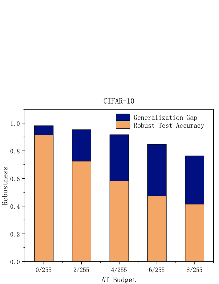
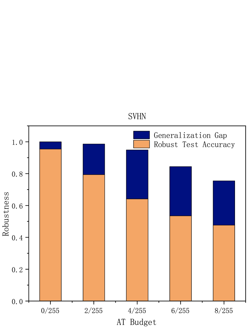
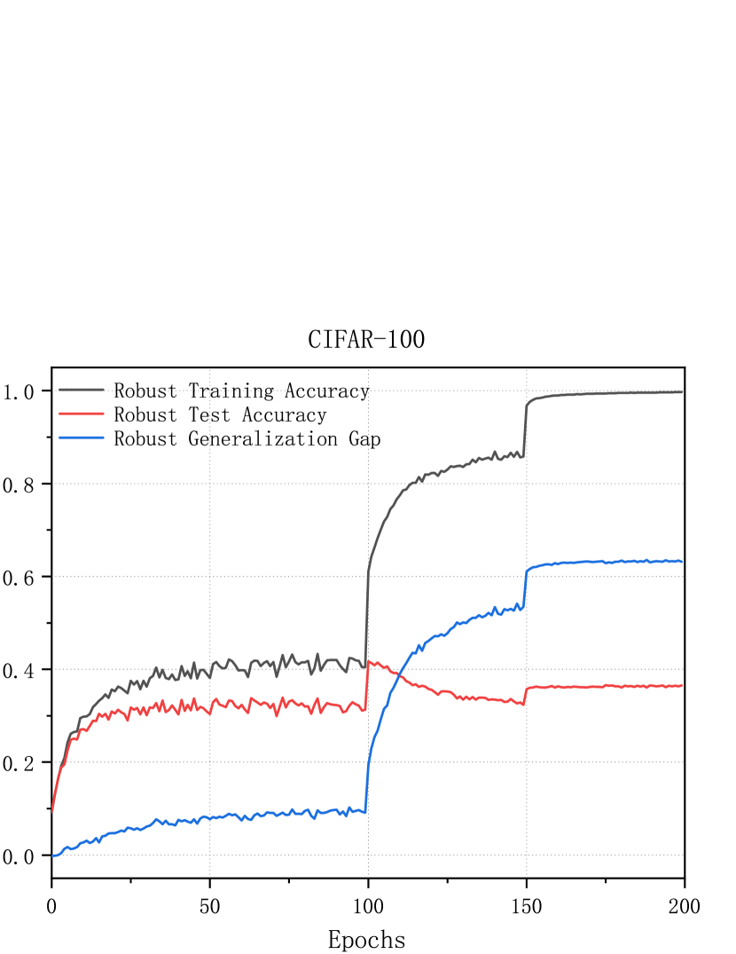
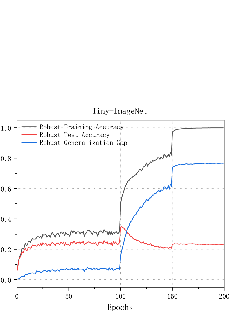
We adversarially train ResNet-18 (He etΒ al. 2016) on CIFAR-10, CIFAR-100 (Krizhevsky, Hinton etΒ al. 2009), SVHN (Netzer etΒ al. 2011), and Tiny-ImageNet (Le and Yang 2015). Figures 1 and 1 show that the robust generalization is more difficult than the standard generalization, i.e. $\epsilon=0$ as shown by Equ. (4) and Equ. (8). The effect of even a small $\epsilon$ such as $2/255$ is amplified by the gradient and Hessian Lipschitz constants in $z$, namely $L_{z}$ and $H_{z}$, and results in a large generalization gap. Moreover, the robust generalization gap increases with $\epsilon$ which implies that it is harder to ensure robustness in a broader area. Figures 2 and 2 present the robust overfitting phenomenon on CIFAR-100 and Tiny-ImageNet. When training errors converge to zero, the robust generalization gaps (blue lines) grow throughout the whole training procedure, while the robust test accuracy (red lines) increases in the first 100 epochs, decreases from the first learning rate decay at the 100-th epoch, and then jumps a little at the 150-th epoch before stabilizes.

Refer to caption

(c) CIFAR-100

Refer to caption

(d) Tiny-ImageNet

Figure 2: The robust overfitting phenomenon.

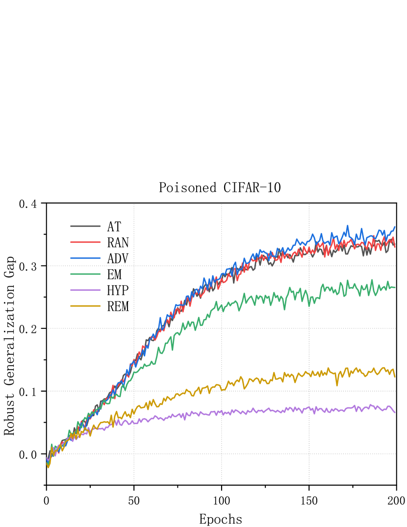
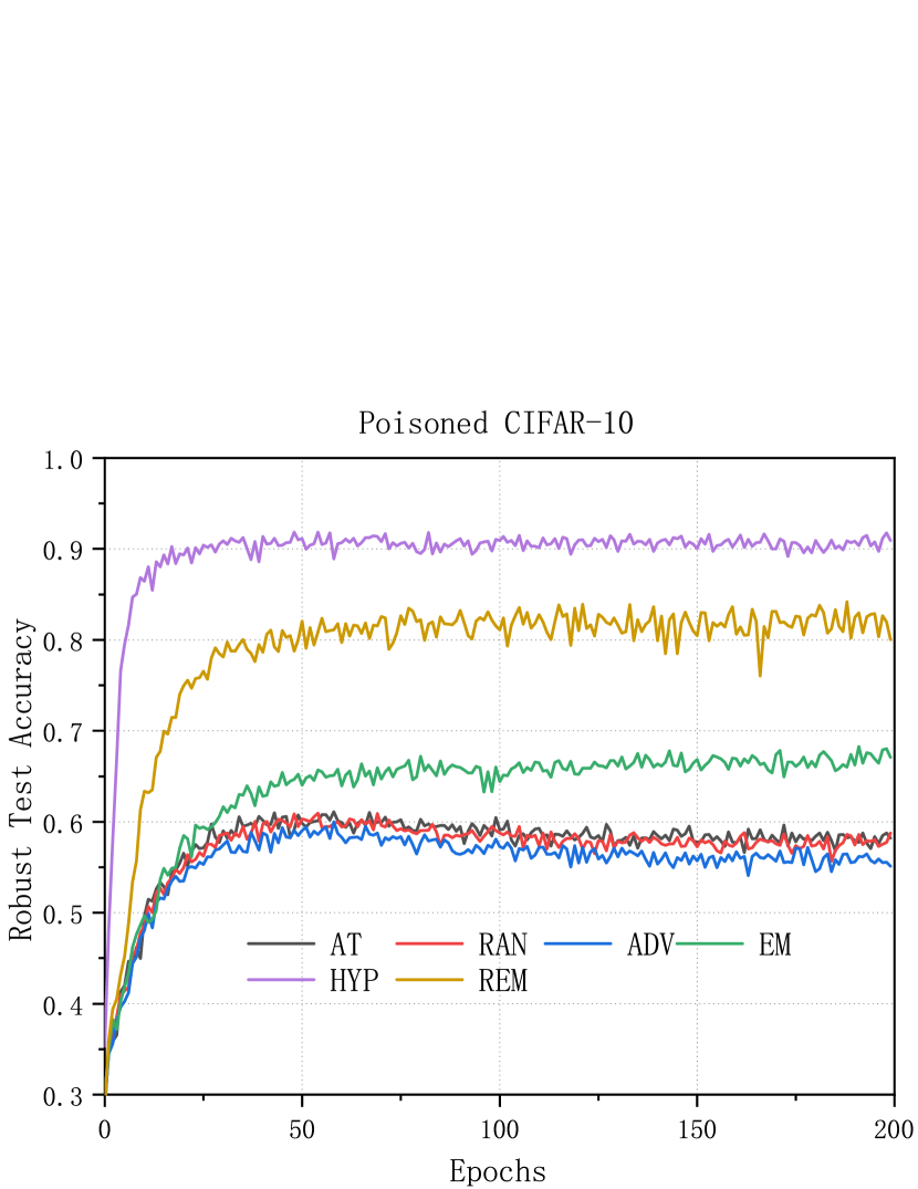
5.2 Poisoned Robust Generalization.

A poisoning attack is called a stability attack if the attack aims at destroying the robustness of a model, trained on the poisoned training set ${{\mathcal{P}}}(S)\sim{{\mathcal{P}}}_{\#}{\mathcal{D}}^{n}$, on the original distribution ${\mathcal{D}}$, i.e. ${\mathcal{R}}_{{\mathcal{D}}}({\mathcal{A}}_{{\mathcal{P}}}(S))$. Stability attacks employed in this paper include the error-minimizing noise (EM) (Huang etΒ al. 2021), the robust error-minimizing noise (REM) (Fu etΒ al. 2022), the adversarial poisoning (ADV) (Fowl etΒ al. 2021), the hypocritical perturbation (HYP) (Tao etΒ al. 2022) and the class-wise random noise (RAN). We poison both the training and test sets to simulate the poisoned distribution ${{\mathcal{P}}}_{\#}{\mathcal{D}}$. Detailed poisoning settings are given in Appendix C.

Refer to caption

(a) Poisoned Gen Gap

Refer to caption

(b) Poisoned Test Acc

Figure 3: The robust generalization and robust test accuracy on poisoned CIFAR-10 under different stability attacks. The adversarial training budget $\epsilon=4/255$ and the poisoning budget $\epsilon^{\prime}=8/255$.

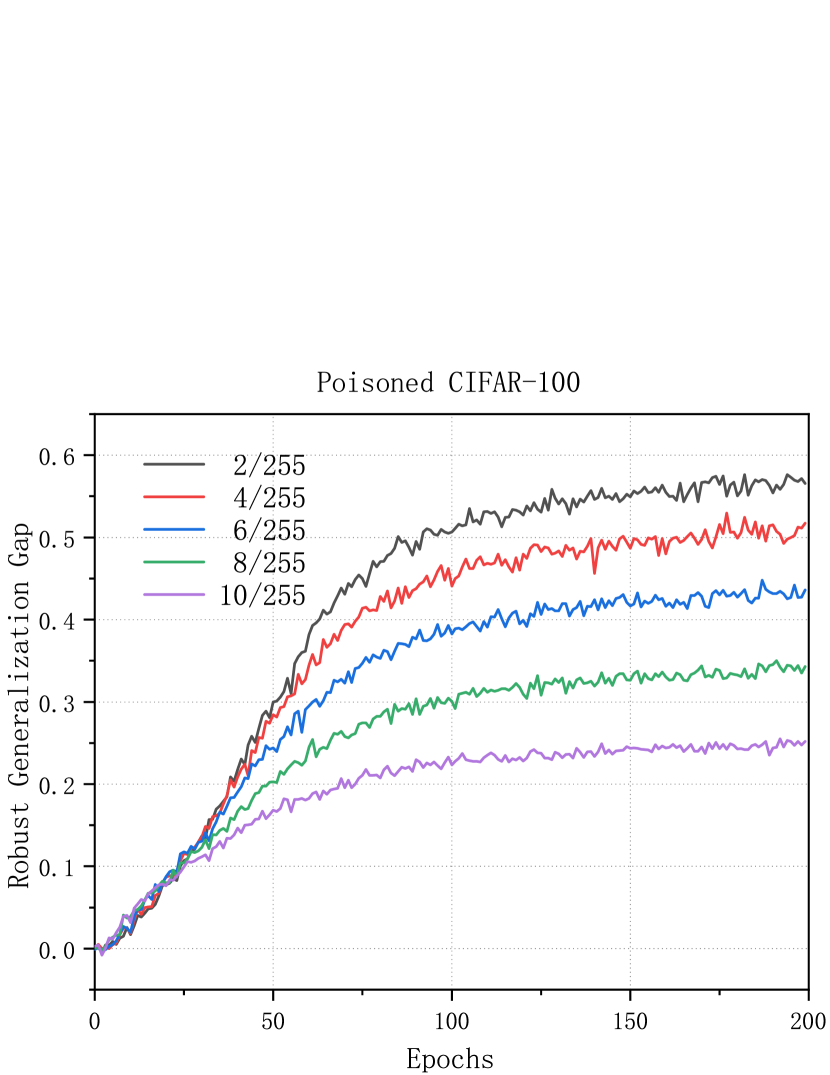
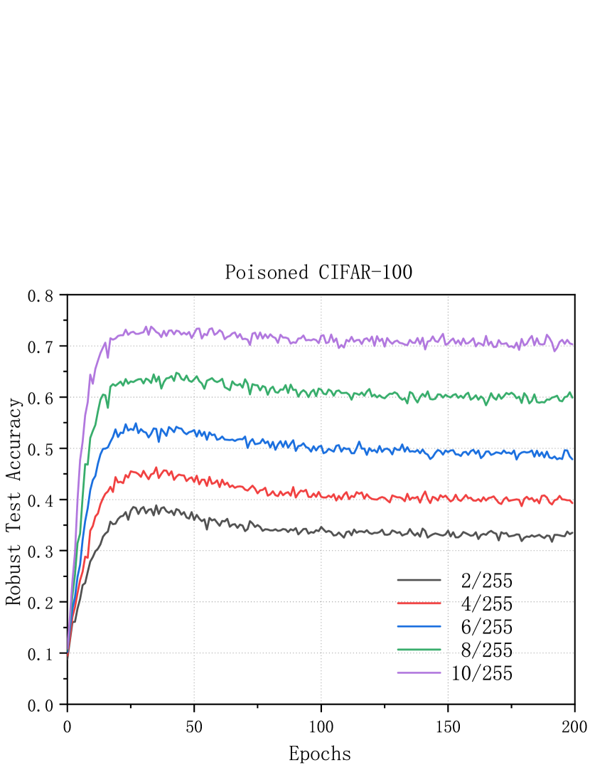
Our bounds reflect the influence of data poisoning on the poisoned robust generalization. First, effective stability attacks such as EM, HYP, and REM, indeed result in the shrinkage of robust generalization gaps on CIFAR-10 and ResNet-18 in Figures 3. Comparing Figure 3 and Figure 3, we see that robust generalization gaps present correlated trends to the test performance as pointed out by our results, i.e. Equ. (8) and (10). We further study the robust generalization under the HYP attack with various intensities, i.e. the poisoning budget $\epsilon^{\prime}$, on CIFAR-100. A larger budget leads to a stronger stability attack. Figure 4 and 4 show that a stronger stability attack results in a lower robust test accuracy as well as a narrower robust generalization gap on the poisoned data distribution, which confirms the principle stated by our results again.

Refer to caption

(a) Poisoned Gen Gap

Refer to caption

(a) Poisoned Test Acc

Figure 4: The robust generalization and robust test accuracy on the poisoned data under HYP attack with different poisoning budgets. The adversarial training budget $\epsilon=4/255$ and the poisoning budget $\epsilon^{\prime}$ varies.

6 Conclusion

Motivated by the need to analyze the generalization ability for adversarial training under data poisoning attacks, we present a data-dependent stability analysis of adversarial training. Precisely, under certain reasonable smoothness conditions on the loss functions, we prove that SGD-based adversarial training is an $\varepsilon({\mathcal{D}},\theta_{1})$-on-average stable randomized algorithm, and thus give an upper bound $\varepsilon({\mathcal{D}},\theta_{1})$ for the robust generalization gap of the training algorithm. The bound $\varepsilon({\mathcal{D}},\theta_{1})$ depends on the data distribution and the initial point of the algorithm and can be used to explain the changes in the poisoned robust generalization gaps of adversarial training.

Limitations and future works

Our theoretical results provide the first attempt to analyze the influence of distribution shifts on robust generalization bounds, but only partial solutions are given. More refined generalization bounds for adversarial training to capture more relationships between robust generalization and distribution are a future research problem. Furthermore, alternative forms of Assumptions 4 and 5 for ReLU-based networks need to be further studied.

References

  • Allen-Zhu, Li, and Song (2019) Allen-Zhu, Z.; Li, Y.; and Song, Z. 2019. A convergence theory for deep learning via over-parameterization. In International Conference on Machine Learning, 242–252.
  • Bassily etΒ al. (2020) Bassily, R.; Feldman, V.; GuzmΓ‘n, C.; and Talwar, K. 2020. Stability of stochastic gradient descent on nonsmooth convex losses. Advances in Neural Information Processing Systems, 33: 4381–4391.
  • Biggio etΒ al. (2013) Biggio, B.; Corona, I.; Maiorca, D.; Nelson, B.; Ε rndiΔ‡, N.; Laskov, P.; Giacinto, G.; and Roli, F. 2013. Evasion attacks against machine learning at test time. In Joint European conference on machine learning and knowledge discovery in databases, 387–402. Springer.
  • Bousquet and Elisseeff (2002) Bousquet, O.; and Elisseeff, A. 2002. Stability and generalization. The Journal of Machine Learning Research, 2: 499–526.
  • Chen etΒ al. (2020) Chen, T.; Zhang, Z.; Liu, S.; Chang, S.; and Wang, Z. 2020. Robust overfitting may be mitigated by properly learned smoothening. In International Conference on Learning Representations.
  • Chen etΒ al. (2022) Chen, T.; Zhang, Z.; Wang, P.; Balachandra, S.; Ma, H.; Wang, Z.; and Wang, Z. 2022. Sparsity Winning Twice: Better Robust Generaliztion from More Efficient Training. arXiv preprint arXiv:2202.09844.
  • Du etΒ al. (2019) Du, S.; Lee, J.; Li, H.; Wang, L.; and Zhai, X. 2019. Gradient descent finds global minima of deep neural networks. In International conference on machine learning, 1675–1685.
  • Farnia and Ozdaglar (2021) Farnia, F.; and Ozdaglar, A. 2021. Train simultaneously, generalize better: Stability of gradient-based minimax learners. In International Conference on Machine Learning, 3174–3185.
  • Feng, Cai, and Zhou (2019) Feng, J.; Cai, Q.-Z.; and Zhou, Z.-H. 2019. Learning to confuse: generating training time adversarial data with auto-encoder. Advances in Neural Information Processing Systems, 32.
  • Fowl etΒ al. (2021) Fowl, L.; Goldblum, M.; Chiang, P.-y.; Geiping, J.; Czaja, W.; and Goldstein, T. 2021. Adversarial examples make strong poisons. arXiv preprint arXiv:2106.10807.
  • Fu etΒ al. (2022) Fu, S.; He, F.; Liu, Y.; Shen, L.; and Tao, D. 2022. Robust Unlearnable Examples: Protecting Data Against Adversarial Learning. arXiv preprint arXiv:2203.14533.
  • Gao, Liu, and Yu (2022) Gao, X.-S.; Liu, S.; and Yu, L. 2022. Achieving Optimal Adversarial Accuracy for Adversarial Deep Learning Using Stackelberg Games. Acta Mathematica Scientia, 42B(6): 2399–2418.
  • Ge etΒ al. (2015) Ge, R.; Huang, F.; Jin, C.; and Yuan, Y. 2015. Escaping from saddle pointsβ€”online stochastic gradient for tensor decomposition. In Conference on learning theory, 797–842.
  • Goodfellow, Shlens, and Szegedy (2014) Goodfellow, I.Β J.; Shlens, J.; and Szegedy, C. 2014. Explaining and harnessing adversarial examples. arXiv preprint arXiv:1412.6572.
  • Gowal etΒ al. (2021) Gowal, S.; Rebuffi, S.-A.; Wiles, O.; Stimberg, F.; Calian, D.Β A.; and Mann, T.Β A. 2021. Improving robustness using generated data. Advances in Neural Information Processing Systems, 34: 4218–4233.
  • Hardt, Recht, and Singer (2016) Hardt, M.; Recht, B.; and Singer, Y. 2016. Train faster, generalize better: Stability of stochastic gradient descent. In International conference on machine learning, 1225–1234.
  • He etΒ al. (2016) He, K.; Zhang, X.; Ren, S.; and Sun, J. 2016. Deep residual learning for image recognition. In Proceedings of the IEEE conference on computer vision and pattern recognition, 770–778.
  • Huang etΒ al. (2021) Huang, H.; Ma, X.; Erfani, S.Β M.; Bailey, J.; and Wang, Y. 2021. Unlearnable examples: Making personal data unexploitable. arXiv preprint arXiv:2101.04898.
  • Ilyas etΒ al. (2019) Ilyas, A.; Santurkar, S.; Tsipras, D.; Engstrom, L.; Tran, B.; and Madry, A. 2019. Adversarial examples are not bugs, they are features. Advances in neural information processing systems, 32.
  • Krizhevsky, Hinton etΒ al. (2009) Krizhevsky, A.; Hinton, G.; etΒ al. 2009. Learning multiple layers of features from tiny images. Technical Report TR-2009.
  • Kuzborskij and Lampert (2018) Kuzborskij, I.; and Lampert, C. 2018. Data-dependent stability of stochastic gradient descent. In International Conference on Machine Learning, 2815–2824.
  • Le and Yang (2015) Le, Y.; and Yang, X. 2015. Tiny imagenet visual recognition challenge. CS 231N, 7(7): 3.
  • Li etΒ al. (2022) Li, B.; Jin, J.; Zhong, H.; Hopcroft, J.; and Wang, L. 2022. Why robust generalization in deep learning is difficult: Perspective of expressive power. Advances in Neural Information Processing Systems, 35: 4370–4384.
  • Liu etΒ al. (2020) Liu, C.; Salzmann, M.; Lin, T.; Tomioka, R.; and SΓΌsstrunk, S. 2020. On the loss landscape of adversarial training: Identifying challenges and how to overcome them. Advances in Neural Information Processing Systems, 33: 21476–21487.
  • Liu etΒ al. (2021) Liu, Z.; Zhao, Z.; Kolmus, A.; Berns, T.; van Laarhoven, T.; Heskes, T.; and Larson, M. 2021. Going Grayscale: The Road to Understanding and Improving Unlearnable Examples. arXiv preprint arXiv:2111.13244.
  • Madry etΒ al. (2017) Madry, A.; Makelov, A.; Schmidt, L.; Tsipras, D.; and Vladu, A. 2017. Towards deep learning models resistant to adversarial attacks. arXiv preprint arXiv:1706.06083.
  • Moosavi-Dezfooli, Fawzi, and Frossard (2016) Moosavi-Dezfooli, S.-M.; Fawzi, A.; and Frossard, P. 2016. Deepfool: a simple and accurate method to fool deep neural networks. In Proceedings of the IEEE conference on computer vision and pattern recognition, 2574–2582.
  • Nemirovski etΒ al. (2009) Nemirovski, A.; Juditsky, A.; Lan, G.; and Shapiro, A. 2009. Robust stochastic approximation approach to stochastic programming. SIAM Journal on Optimization, 19(4): 1574–1609.
  • Netzer etΒ al. (2011) Netzer, Y.; Wang, T.; Coates, A.; Bissacco, A.; Wu, B.; and Ng, A.Β Y. 2011. Reading digits in natural images with unsupervised feature learning. In NIPS DLW.
  • Nguyen, Yosinski, and Clune (2015) Nguyen, A.; Yosinski, J.; and Clune, J. 2015. Deep neural networks are easily fooled: High confidence predictions for unrecognizable images. In Proceedings of the IEEE conference on computer vision and pattern recognition, 427–436.
  • Ren etΒ al. (2022) Ren, J.; Xu, H.; Wan, Y.; Ma, X.; Sun, L.; and Tang, J. 2022. Transferable Unlearnable Examples. arXiv preprint arXiv:2210.10114.
  • Rice, Wong, and Kolter (2020) Rice, L.; Wong, E.; and Kolter, Z. 2020. Overfitting in adversarially robust deep learning. In International Conference on Machine Learning, 8093–8104.
  • Schmidt etΒ al. (2018) Schmidt, L.; Santurkar, S.; Tsipras, D.; Talwar, K.; and Madry, A. 2018. Adversarially robust generalization requires more data. Advances in neural information processing systems, 31.
  • Shaham, Yamada, and Negahban (2015) Shaham, U.; Yamada, Y.; and Negahban, S. 2015. Understanding adversarial training: Increasing local stability of neural nets through robust optimization. arXiv preprint arXiv:1511.05432.
  • Shalev-Shwartz etΒ al. (2010) Shalev-Shwartz, S.; Shamir, O.; Srebro, N.; and Sridharan, K. 2010. Learnability, stability and uniform convergence. The Journal of Machine Learning Research, 11: 2635–2670.
  • Sinha etΒ al. (2017) Sinha, A.; Namkoong, H.; Volpi, R.; and Duchi, J. 2017. Certifying some distributional robustness with principled adversarial training. arXiv preprint arXiv:1710.10571.
  • Szegedy etΒ al. (2013) Szegedy, C.; Zaremba, W.; Sutskever, I.; Bruna, J.; Erhan, D.; Goodfellow, I.; and Fergus, R. 2013. Intriguing properties of neural networks. arXiv preprint arXiv:1312.6199.
  • Tao etΒ al. (2022) Tao, L.; Feng, L.; Wei, H.; Yi, J.; Huang, S.-J.; and Chen, S. 2022. Can Adversarial Training Be Manipulated By Non-Robust Features? arXiv preprint arXiv:2201.13329.
  • Tao etΒ al. (2021) Tao, L.; Feng, L.; Yi, J.; Huang, S.-J.; and Chen, S. 2021. Better safe than sorry: Preventing delusive adversaries with adversarial training. Advances in Neural Information Processing Systems, 34: 16209–16225.
  • Wang etΒ al. (2019) Wang, Y.; Zou, D.; Yi, J.; Bailey, J.; Ma, X.; and Gu, Q. 2019. Improving adversarial robustness requires revisiting misclassified examples. In International Conference on Learning Representations.
  • Wang etΒ al. (2023) Wang, Z.; Pang, T.; Du, C.; Lin, M.; Liu, W.; and Yan, S. 2023. Better diffusion models further improve adversarial training. arXiv preprint arXiv:2302.04638.
  • Wang, Wang, and Wang (2021) Wang, Z.; Wang, Y.; and Wang, Y. 2021. Fooling Adversarial Training with Inducing Noise. arXiv preprint arXiv:2111.10130.
  • Wu, Xia, and Wang (2020) Wu, D.; Xia, S.-T.; and Wang, Y. 2020. Adversarial weight perturbation helps robust generalization. Advances in Neural Information Processing Systems, 33: 2958–2969.
  • Xiao etΒ al. (2022) Xiao, J.; Fan, Y.; Sun, R.; Wang, J.; and Luo, Z.-Q. 2022. Stability analysis and generalization bounds of adversarial training. arXiv preprint arXiv:2210.00960.
  • Xing, Song, and Cheng (2021) Xing, Y.; Song, Q.; and Cheng, G. 2021. On the algorithmic stability of adversarial training. Advances in Neural Information Processing Systems, 34: 26523–26535.
  • Yu etΒ al. (2022a) Yu, C.; Han, B.; Shen, L.; Yu, J.; Gong, C.; Gong, M.; and Liu, T. 2022a. Understanding robust overfitting of adversarial training and beyond. In International Conference on Machine Learning, 25595–25610.
  • Yu etΒ al. (2022b) Yu, D.; Zhang, H.; Chen, W.; Yin, J.; and Liu, T.-Y. 2022b. Availability attacks create shortcuts. In Proceedings of the 28th ACM SIGKDD Conference on Knowledge Discovery and Data Mining, 2367–2376.
  • Zhang etΒ al. (2019) Zhang, H.; Yu, Y.; Jiao, J.; Xing, E.; ElΒ Ghaoui, L.; and Jordan, M. 2019. Theoretically principled trade-off between robustness and accuracy. In International conference on machine learning, 7472–7482.

Appendix A Proofs

A.1 Proof of Lemma 8

Proof.
  1. 1.

    Assume that $h(\theta_{1},z)=l(\theta_{1},z_{1})$ and $h(\theta_{2},z)=l(\theta_{2},z_{2})$. We have

    $\displaystyle||h(\theta_{1},z)-h(\theta_{2},z)||=||l(\theta_{1},z_{1})-l(\theta_{2},z_{2})||.$

    Note that $l(\theta_{1},z_{1})\geq l(\theta_{1},z_{2})$ and $l(\theta_{2},z_{2})\geq l(\theta_{2},z_{1})$.
    If $l(\theta_{1},z_{1})\geq l(\theta_{2},z_{2})$, then

    $\displaystyle||l(\theta_{1},z_{1})-l(\theta_{2},z_{2})||\leq l(\theta_{1},z_{1})-l(\theta_{2},z_{1})\leq L||\theta_{1}-\theta_{2}||.$

    If $l(\theta_{1},z_{1})\leq l(\theta_{2},z_{2})$, then

    $\displaystyle||l(\theta_{1},z_{1})-l(\theta_{2},z_{2})||\leq l(\theta_{2},z_{2})-l(\theta_{1},z_{2})\leq L||\theta_{1}-\theta_{2}||.$
  2. 2.

    Assume that $h(\theta_{1},z)=l(\theta_{1},z_{1})$ and $h(\theta_{2},z)=l(\theta_{2},z_{2})$.

    $\displaystyle||\nabla h(\theta_{1},z)-\nabla h(\theta_{2},z)||$
    $\displaystyle=$ $\displaystyle||\nabla l(\theta_{1},z_{1})-\nabla l(\theta_{2},z_{2})||$
    $\displaystyle\leq$ $\displaystyle||\nabla l(\theta_{1},z_{1})-\nabla l(\theta_{1},z_{2})||+||\nabla l(\theta_{1},z_{2})-\nabla l(\theta_{2},z_{2})||$
    $\displaystyle\leq$ $\displaystyle L_{\theta}||\theta_{1}-\theta_{2}||+L_{z}||z_{1}-z_{2}||_{p}$
    $\displaystyle\leq$ $\displaystyle L_{\theta}||\theta_{1}-\theta_{2}||+2\epsilon L_{z}.$
  3. 3.

    Assume that $h(\theta_{1},z)=l(\theta_{1},z_{1})$ and $h(\theta_{2},z)=l(\theta_{2},z_{2})$.

    $\displaystyle||\nabla^{2}h(\theta_{1},z)-\nabla^{2}h(\theta_{2},z)||$
    $\displaystyle=$ $\displaystyle||\nabla^{2}l(\theta_{1},z_{1})-\nabla^{2}l(\theta_{2},z_{2})||$
    $\displaystyle\leq$ $\displaystyle||\nabla^{2}l(\theta_{1},z_{1})-\nabla^{2}l(\theta_{1},z_{2})||+||\nabla^{2}l(\theta_{1},z_{2})-\nabla^{2}l(\theta_{2},z_{2})||$
    $\displaystyle\leq$ $\displaystyle H_{\theta}||\theta_{1}-\theta_{2}||+H_{z}||z_{1}-z_{2}||_{p}$
    $\displaystyle\leq$ $\displaystyle H_{\theta}||\theta_{1}-\theta_{2}||+2\epsilon H_{z}.$

∎

A.2 Proof of Theorem 9

We first prove several lemmas. A core technique in stability analysis is to give the expansion properties of update rules.

Definition 14 (Expansion).

The update rule ${\mathcal{G}}_{\mathcal{A}}$ is $\iota$-approximately $\kappa$-expansive, if $\forall z\in{\mathbb{D}}$

$\displaystyle||{\mathcal{G}}_{\mathcal{A}}(\theta_{1},z,\alpha)-{\mathcal{G}}_{\mathcal{A}}(\theta_{2},z,\alpha)||\leq\kappa||\theta_{1}-\theta_{2}||+\iota.$

If the original loss $l(\theta,z)$ is $\beta$-gradient Lipschitz in $\theta$, then the update rule in standard training is $1$-expansive in the convex case and $(1+\alpha\beta)$-expansive in the non-convex case (Hardt, Recht, and Singer 2016). If the adversarial loss $h(\theta,z)$ is $\eta$-approximately $\beta$-gradient Lipschitz in $\theta$, then the expansion coefficients in the update rule ${\mathcal{G}}_{\mathcal{A}}$ remain unchanged in both convex and non-convex cases, while the approximation parameter $\eta$ leads to an additional term $\alpha\eta$ in each update (Xiao etΒ al. 2022).

Lemma 15 ( Xiao etΒ al. (2022)).

Suppose the adversarial loss $h(\theta,z)$ is $\eta$-approximately $\beta$-gradient Lipschitz in $\theta$.

  1. 1.

    ($\eta$-approximate descent.)

    $\displaystyle h(\theta_{1},z)-h(\theta_{2},z)\leq\nabla h(\theta_{2},z)^{\top}(\theta_{1}-\theta_{2})+\frac{\beta}{2}||\theta_{1}-\theta_{2}||^{2}+\eta||\theta_{1}-\theta_{2}||.$
  2. 2.

    The update rule ${\mathcal{G}}_{\mathcal{A}}$ is $\eta$-approximately $(1+\alpha\beta)$-expansive:

    $\displaystyle||{\mathcal{G}}_{\mathcal{A}}(\theta_{1},z,\alpha)-{\mathcal{G}}_{\mathcal{A}}(\theta_{2},z,\alpha)||\leq(1+\alpha\beta)||\theta_{1}-\theta_{2}||+\alpha\eta.$
  3. 3.

    Assume in addition that $h(\theta,z)$ is convex in $\theta$, for $\alpha\leq 1/\beta$, we have

    $\displaystyle||{\mathcal{G}}_{\mathcal{A}}(\theta_{1},z,\alpha)-{\mathcal{G}}_{\mathcal{A}}(\theta_{2},z,\alpha)||\leq||\theta_{1}-\theta_{2}||+\alpha\eta.$

Given a data set $S=\{z_{1},\cdots,z_{n}\}\sim{\mathcal{D}}^{n}$, an example $z\sim{\mathcal{D}}$, and an index $i\in[n]$, we denote $S^{i,z}=\{z^{\prime}_{1},\cdots,z^{\prime}_{n}\}$ with $z^{\prime}_{j}=z_{j}$ for jβ‰ i𝑗𝑖j\neq i and $z^{\prime}_{i}=z$. Let $\theta_{t}$, $\theta_{t}^{\prime}$ be the $t$-th outputs of ${\mathcal{A}}(S)$ and ${\mathcal{A}}(S^{i,z})$ respectively. Denote the distance of two trajectories at step $t$ by $\delta_{t}(S,z,i,{\mathcal{A}})=||\theta_{t}-\theta_{t}^{\prime}||$. As both two updates start from $\theta_{1}$, we have $\delta_{1}(S,z,i,{\mathcal{A}})=0$. Since the on-average stability in Definition 1 takes supremum over the index $i\in[n]$, the stability analysis aims at providing a unified bound for all $i\in[n]$. Thus, we will not point out the selection of $i$ in later statements for brevity.

We restate Lemma 5 in (Kuzborskij and Lampert 2018) on which the data-dependent stability analysis relies. Note that this lemma holds for SGD without replacement in both a single pass and multiple passes through the training set. The multiple-pass case cycles through $S$ repeatedly in a fixed order determined by ${\mathcal{A}}$.

Lemma 16.

Assume the adversarial loss $h(\theta,z)$ is non-negative and $L$-Lipschitz in $\theta$. Then, $\forall t_{0}\in[n+1]$,

$\displaystyle\mathop{\mathbb{E}}_{S,z,{\mathcal{A}}}[h(\theta_{t},z)-h(\theta_{t}^{\prime},z)]\leq L\mathop{\mathbb{E}}_{S,z}[\mathop{\mathbb{E}}_{\mathcal{A}}[\delta_{t}(S,z,i,{\mathcal{A}})|\delta_{t_{0}}(S,z,i,{\mathcal{A}})=0]]+\frac{t_{0}-1}{n}\mathop{\mathbb{E}}_{S,{\mathcal{A}}}[{\mathcal{R}}_{\mathcal{D}}(\theta_{t})].$

Due to the change of notations, we repeat the proof here.

Proof.

By the Lipschitz condition and non-negativeness of $h$, we have

$\displaystyle h(\theta_{t},z)-h(\theta^{\prime}_{t},z)$
$\displaystyle=$ (h​(ΞΈt,z)βˆ’h​(ΞΈtβ€²,z))​𝕀​{Ξ΄t0​(S,z,i,π’œ)=0}+(h​(ΞΈt,z)βˆ’h​(ΞΈtβ€²,z))​𝕀​{Ξ΄t0​(S,z,i,π’œ)β‰ 0}β„Žsubscriptπœƒπ‘‘π‘§β„Žsubscriptsuperscriptπœƒβ€²π‘‘π‘§π•€subscript𝛿subscript𝑑0π‘†π‘§π‘–π’œ0β„Žsubscriptπœƒπ‘‘π‘§β„Žsubscriptsuperscriptπœƒβ€²π‘‘π‘§π•€subscript𝛿subscript𝑑0π‘†π‘§π‘–π’œ0\displaystyle(h(\theta_{t},z)-h(\theta^{\prime}_{t},z)){\mathbb{I}}\{\delta_{t_{0}}(S,z,i,{\mathcal{A}})=0\}+(h(\theta_{t},z)-h(\theta^{\prime}_{t},z)){\mathbb{I}}\{\delta_{t_{0}}(S,z,i,{\mathcal{A}})\neq 0\}
$\displaystyle\leq$ L​δt​(S,z,i,π’œ)​𝕀​{Ξ΄t0​(S,z,i,π’œ)=0}+h​(ΞΈt,z)​𝕀​{Ξ΄t0​(S,z,i,π’œ)β‰ 0}.𝐿subscriptπ›Ώπ‘‘π‘†π‘§π‘–π’œπ•€subscript𝛿subscript𝑑0π‘†π‘§π‘–π’œ0β„Žsubscriptπœƒπ‘‘π‘§π•€subscript𝛿subscript𝑑0π‘†π‘§π‘–π’œ0\displaystyle L\delta_{t}(S,z,i,{\mathcal{A}}){\mathbb{I}}\{\delta_{t_{0}}(S,z,i,{\mathcal{A}})=0\}+h(\theta_{t},z){\mathbb{I}}\{\delta_{t_{0}}(S,z,i,{\mathcal{A}})\neq 0\}.

Take expectation w.r.t. ${\mathcal{A}}$ and we have

π”Όπ’œ[h​(ΞΈt,z)βˆ’h​(ΞΈtβ€²,z)]≀Lβ€‹π”Όπ’œ[Ξ΄t​(S,z,i,π’œ)|Ξ΄t0​(S,z,i,π’œ)=0]+π”Όπ’œ[h​(ΞΈt,z)​𝕀​{Ξ΄t0​(S,z,i,π’œ)β‰ 0}].subscriptπ”Όπ’œdelimited-[]β„Žsubscriptπœƒπ‘‘π‘§β„Žsubscriptsuperscriptπœƒβ€²π‘‘π‘§πΏsubscriptπ”Όπ’œdelimited-[]conditionalsubscriptπ›Ώπ‘‘π‘†π‘§π‘–π’œsubscript𝛿subscript𝑑0π‘†π‘§π‘–π’œ0subscriptπ”Όπ’œdelimited-[]β„Žsubscriptπœƒπ‘‘π‘§π•€subscript𝛿subscript𝑑0π‘†π‘§π‘–π’œ0\displaystyle\mathop{\mathbb{E}}_{\mathcal{A}}[h(\theta_{t},z)-h(\theta^{\prime}_{t},z)]\leq L\mathop{\mathbb{E}}_{\mathcal{A}}[\delta_{t}(S,z,i,{\mathcal{A}})|\delta_{t_{0}}(S,z,i,{\mathcal{A}})=0]+\mathop{\mathbb{E}}_{\mathcal{A}}[h(\theta_{t},z){\mathbb{I}}\{\delta_{t_{0}}(S,z,i,{\mathcal{A}})\neq 0\}]. (12)

Note that the first time that ${\mathcal{A}}$ selects the different example is $\pi^{-1}(i)$. Since that $\pi^{-1}(i)\geq t_{0}$ implies $\delta_{t_{0}}(S,z,i,{\mathcal{A}})=0$, we have 𝕀​{Ξ΄t0​(S,z,i,π’œ)β‰ 0}≀𝕀​{Ο€βˆ’1​(i)<t0}𝕀subscript𝛿subscript𝑑0π‘†π‘§π‘–π’œ0𝕀superscriptπœ‹1𝑖subscript𝑑0{\mathbb{I}}\{\delta_{t_{0}}(S,z,i,{\mathcal{A}})\neq 0\}\leq{\mathbb{I}}\{\pi^{-1}(i)<t_{0}\}. It follows that

𝔼S,z[π”Όπ’œ[h(ΞΈt,z)𝕀{Ξ΄t0(S,z,i,π’œ)β‰ 0}]]]\displaystyle\mathop{\mathbb{E}}_{S,z}[\mathop{\mathbb{E}}_{\mathcal{A}}[h(\theta_{t},z){\mathbb{I}}\{\delta_{t_{0}}(S,z,i,{\mathcal{A}})\neq 0\}]]]
$\displaystyle\leq\mathop{\mathbb{E}}_{S,z}[\mathop{\mathbb{E}}_{\mathcal{A}}[h(\theta_{t},z){\mathbb{I}}\{\pi^{-1}(i)<t_{0}\}]]$
$\displaystyle=\mathop{\mathbb{E}}_{z,{\mathcal{A}}}[\mathop{\mathbb{E}}_{S}[h(\theta_{t},z)]{\mathbb{I}}\{\pi^{-1}(i)<t_{0}\}].$ (13)

Recall that a realization of ${\mathcal{A}}$ is a permutation $\pi$ of $[n]$. Thus, with a fixed $\pi$, taking over $S\sim{\mathcal{D}}^{n}$ equals to taking over both $S\sim{\mathcal{D}}^{n}$ and ${\mathcal{A}}$. That is, $\mathop{\mathbb{E}}_{S}[h(\theta_{t},z)]=\mathop{\mathbb{E}}_{{\mathcal{A}},S}[h(\theta_{t},z)]$. As a consequence, we have

$\displaystyle\mathop{\mathbb{E}}_{z,{\mathcal{A}}}[\mathop{\mathbb{E}}_{S}[h(\theta_{t},z)]{\mathbb{I}}\{\pi^{-1}(i)<t_{0}\}]$ (14)
$\displaystyle=$ $\displaystyle\mathop{\mathbb{E}}_{S,z,{\mathcal{A}}}[h(\theta_{t},z)]\mathop{\mathbb{E}}_{{\mathcal{A}}}[{\mathbb{I}}\{\pi^{-1}(i)<t_{0}\}]$
$\displaystyle\leq$ $\displaystyle\frac{t_{0}-1}{n}\mathop{\mathbb{E}}_{S,z,{\mathcal{A}}}[h(\theta_{t},z)].$ (15)

Combining Equation (12)  (13) and  (15), we get the statement. ∎

Lemma 17.

Suppose the adversarial loss $h(\theta,z)$ is $L$-Lipschitz and $\eta$-approximately $\beta$-gradient Lipschitz in $\theta$. Then, in a single pass such that $T\in[n]$, we have that

$\displaystyle\sum_{t=1}^{T}(\alpha_{t}-\frac{\beta\alpha_{t}^{2}}{2})\mathop{\mathbb{E}}_{S}[||\nabla{\mathcal{R}}_{\mathcal{D}}(\theta_{t})||^{2}]\leq{\mathcal{R}}_{\mathcal{D}}(\theta_{1})-\mathop{\mathbb{E}}_{S}[{\mathcal{R}}_{\mathcal{D}}(\theta_{T})]+\eta L\sum_{t=1}^{T}\alpha_{t}+\frac{\beta}{2}\sum_{t=1}^{T}\alpha_{t}^{2}\mathop{\mathbb{E}}_{S}[||\nabla h(\theta_{t},z_{\pi(t)})-\nabla{\mathcal{R}}_{\mathcal{D}}(\theta_{t})||^{2}].$
Proof.

From the first statement in Lemma 15, we have

$\displaystyle{\mathcal{R}}_{\mathcal{D}}(\theta_{t+1})-{\mathcal{R}}_{\mathcal{D}}(\theta_{t})$
$\displaystyle\leq$ $\displaystyle\nabla{\mathcal{R}}_{\mathcal{D}}(\theta_{t})^{\top}(\theta_{t+1}-\theta_{t})+\frac{\beta\alpha_{t}^{2}}{2}||\nabla h(\theta_{t},z_{\pi(t)})||^{2}+\eta\alpha_{t}||\nabla h(\theta_{t},z_{\pi(t)})||$
$\displaystyle\leq$ $\displaystyle(\beta\alpha_{t}^{2}-\alpha_{t})\nabla{\mathcal{R}}_{\mathcal{D}}(\theta_{t})^{\top}\nabla h(\theta_{t},z_{\pi(t)})+\eta\alpha_{t}L+\frac{\beta\alpha_{t}^{2}}{2}||\nabla h(\theta_{t},z_{\pi(t)})-\nabla{\mathcal{R}}_{\mathcal{D}}(\theta_{t})||^{2}-\frac{\beta\alpha_{t}^{2}}{2}||\nabla{\mathcal{R}}_{\mathcal{D}}(\theta_{t})||^{2}.$

Since $\theta_{t}$ is determined by $z_{\pi(1)},\cdots,z_{\pi(t-1)}$ and $\mathop{\mathbb{E}}_{z_{\pi(t)}}[h(\theta_{t},z_{\pi(t)})]={\mathcal{R}}_{\mathcal{D}}(\theta_{t})$, we have that

$\displaystyle\mathop{\mathbb{E}}_{S}[\nabla{\mathcal{R}}_{\mathcal{D}}(\theta_{t})^{\top}\nabla h(\theta_{t},z_{\pi(t)})]=\mathop{\mathbb{E}}_{S}[||\nabla{\mathcal{R}}_{\mathcal{D}}(\theta_{t})||^{2}].$

Take expectation w.r.t. $S$ and rearrange terms,

$\displaystyle(\alpha_{t}-\frac{\beta\alpha_{t}^{2}}{2})\mathop{\mathbb{E}}_{S}[||\nabla{\mathcal{R}}_{\mathcal{D}}(\theta_{t})||^{2}]\leq\mathop{\mathbb{E}}_{S}[{\mathcal{R}}_{\mathcal{D}}(\theta_{t})-{\mathcal{R}}_{\mathcal{D}}(\theta_{t+1})+\frac{\beta\alpha_{t}^{2}}{2}||\nabla h(\theta_{t},z_{\pi(t)})-\nabla{\mathcal{R}}_{\mathcal{D}}(\theta_{t})||^{2}]+\eta\alpha_{t}L.$

Sum the above over $t=1,\cdots,T$ and get the statement. ∎

Lemma 18.

Suppose the adversarial loss $h(\theta,z)$ is $L$-Lipschitz and $\eta$-approximately $\beta$-gradient Lipschitz with respect to $\theta$, and the step sizes $\alpha_{t}\leq 1/\beta$. Assume the variance of stochastic gradients in ${\mathcal{A}}$ obeys for all $t\in[T]$

$\displaystyle\mathop{\mathbb{E}}_{S}[||\nabla h(\theta_{t},z_{\pi(t)})-\nabla{\mathcal{R}}_{\mathcal{D}}(\theta_{t})||^{2}]\leq\sigma_{t}^{2}.$

We have

$\displaystyle\mathop{\mathbb{E}}_{S}[\sum_{t=1}^{T}\alpha_{t}||\nabla h(\theta_{t},z_{\pi(t)})||]\leq\sum_{t=1}^{T}\sigma_{t}\alpha_{t}+2\sqrt{\sum_{t=1}^{T}\alpha_{t}}\sqrt{{\mathcal{R}}_{\mathcal{D}}(\theta_{1})-{\mathcal{R}}_{\mathcal{D}}(\theta^{*})+\frac{\beta}{2}\sum_{t=1}^{T}\sigma_{t}^{2}\alpha_{t}^{2}+\eta L\sum_{t=1}^{T}\alpha_{t}}$
Proof.

Repeatedly applying Jensen’s inequality, we have

$\displaystyle\mathop{\mathbb{E}}_{S}[\sum_{t=1}^{T}\alpha_{t}||\nabla h(\theta_{t},z_{\pi(t)})||]$
$\displaystyle\leq$ $\displaystyle\sum_{t=1}^{T}\alpha_{t}\mathop{\mathbb{E}}_{S}[||\nabla h(\theta_{t},z_{\pi(t)})-\nabla{\mathcal{R}}_{\mathcal{D}}(\theta_{t})||]+\sum_{t=1}^{T}\alpha_{t}\mathop{\mathbb{E}}_{S}[||\nabla{\mathcal{R}}_{\mathcal{D}}(\theta_{t})||]$
$\displaystyle\leq$ $\displaystyle\sum_{t=1}^{T}\alpha_{t}\sqrt{\mathop{\mathbb{E}}_{S}[||\nabla h(\theta_{t},z_{\pi(t)})-\nabla{\mathcal{R}}_{\mathcal{D}}(\theta_{t})||^{2}]}+\sum_{t=1}^{T}\alpha_{t}\sqrt{\mathop{\mathbb{E}}_{S}[||\nabla{\mathcal{R}}_{\mathcal{D}}(\theta_{t})||^{2}]}$
$\displaystyle\leq$ $\displaystyle\sum_{t=1}^{T}\sigma_{t}\alpha_{t}+\sum_{t=1}^{T}\alpha_{t}\sqrt{\mathop{\mathbb{E}}_{S}[||\nabla{\mathcal{R}}_{\mathcal{D}}(\theta_{t})||^{2}]}$
$\displaystyle\leq$ $\displaystyle\sum_{t=1}^{T}\sigma_{t}\alpha_{t}+2\sum_{t=1}^{T}(\alpha_{t}-\frac{\beta\alpha_{t}^{2}}{2})\sqrt{\mathop{\mathbb{E}}_{S}[||\nabla{\mathcal{R}}_{\mathcal{D}}(\theta_{t})||^{2}]}$
$\displaystyle\leq$ $\displaystyle\sum_{t=1}^{T}\sigma_{t}\alpha_{t}+2\sqrt{\sum_{t=1}^{T}(\alpha_{t}-\frac{\beta\alpha_{t}^{2}}{2})}\sqrt{\sum_{t=1}^{T}(\alpha_{t}-\frac{\beta\alpha_{t}^{2}}{2})\mathop{\mathbb{E}}_{S}[||\nabla{\mathcal{R}}_{\mathcal{D}}(\theta_{t})||^{2}]}$
$\displaystyle\leq$ $\displaystyle\sum_{t=1}^{T}\sigma_{t}\alpha_{t}+2\sqrt{\sum_{t=1}^{T}\alpha_{t}}\sqrt{{\mathcal{R}}_{\mathcal{D}}(\theta_{1})-{\mathcal{R}}_{\mathcal{D}}(\theta^{*})+\frac{\beta}{2}\sum_{t=1}^{T}\sigma_{t}^{2}\alpha_{t}^{2}+\eta L\sum_{t=1}^{T}\alpha_{t}}.$

The penultimate inequality is by Lemma 17. ∎

We now prove Theorem 9.

Proof.

Denote $\Delta_{t}(S,z,i)=\mathop{\mathbb{E}}_{\mathcal{A}}[\delta_{t}(S,z,i,{\mathcal{A}})|\delta_{t_{0}}(S,z,i,{\mathcal{A}})=0]$. By Lemma 16, $\forall t_{0}\in\{1,\cdots,n,n+1\}$ we have

$\displaystyle\mathop{\mathbb{E}}_{S,z,{\mathcal{A}}}[h(\theta_{T+1},z)-h(\theta_{T+1}^{\prime},z)]$
$\displaystyle\leq$ $\displaystyle L\mathop{\mathbb{E}}_{S,z}[\Delta_{T+1}(S,z,i)]+\frac{t_{0}-1}{n}\mathop{\mathbb{E}}_{S,{\mathcal{A}}}[{\mathcal{R}}_{\mathcal{D}}(\theta_{T+1})].$

At step $t$, ${\mathcal{A}}$ selects the example $\pi(t)=i$ with probability $1/n$ and π​(t)β‰ iπœ‹π‘‘π‘–\pi(t)\neq i with probability $1-1/n$. When π​(t)β‰ iπœ‹π‘‘π‘–\pi(t)\neq i, by the third statement in Lemma 15 , we have

$\displaystyle\delta_{t+1}(S,z,i,{\mathcal{A}})\cdot{\mathbb{I}}\{\delta_{t_{0}}(S,z,i,{\mathcal{A}})=0\}$
$\displaystyle\leq$ $\displaystyle\delta_{t}(S,z,i,{\mathcal{A}})\cdot{\mathbb{I}}\{\delta_{t_{0}}(S,z,i,{\mathcal{A}})=0\}+\alpha_{t}\eta.$

When $\pi(t)=i$, we have

$\displaystyle\delta_{t+1}(S,z,i,{\mathcal{A}})\cdot{\mathbb{I}}\{\delta_{t_{0}}(S,z,i,{\mathcal{A}})=0\}$
$\displaystyle\leq$ $\displaystyle\delta_{t}(S,z,i,{\mathcal{A}})\cdot{\mathbb{I}}\{\delta_{t_{0}}(S,z,i,{\mathcal{A}})=0\}+\alpha_{t}||\nabla h(\theta_{t},z_{\pi(t)})||+\alpha_{t}||\nabla h(\theta_{t}^{\prime},z^{\prime}_{\pi(t)})||.$

Take expectation w.r.t. ${\mathcal{A}}$ and we have

$\displaystyle\Delta_{t+1}(S,z,i)$
$\displaystyle\leq$ $\displaystyle\frac{1}{n}(\Delta_{t}(S,z,i)+\alpha_{t}\mathop{\mathbb{E}}_{\mathcal{A}}[||\nabla h(\theta_{t},z_{\pi(t)})||+||\nabla h(\theta_{t}^{\prime},z^{\prime}_{\pi(t)})||])+(1-\frac{1}{n})(\Delta_{t}(S,z,i)+\alpha_{t}\eta)$
$\displaystyle=$ $\displaystyle\Delta_{t}(S,z,i)+(1-\frac{1}{n})\alpha_{t}\eta+\frac{\alpha_{t}}{n}\mathop{\mathbb{E}}_{\mathcal{A}}[||\nabla h(\theta_{t},z_{\pi(t)})||+||\nabla h(\theta_{t}^{\prime},z^{\prime}_{\pi(t)})||].$

Thus, we have

$\displaystyle\mathop{\mathbb{E}}_{S,z,{\mathcal{A}}}[h(\theta_{T+1},z)-h(\theta_{T+1}^{\prime},z)]$
$\displaystyle\leq$ $\displaystyle\frac{L}{n}\sum_{t=t_{0}}^{T}\alpha_{t}\mathop{\mathbb{E}}_{z,{\mathcal{A}}}[\mathop{\mathbb{E}}_{S}[||\nabla h(\theta_{t},z_{\pi(t)})||+||\nabla h(\theta_{t}^{\prime},z^{\prime}_{\pi(t)})||]]+(1-\frac{1}{n})L\eta\sum_{t=t_{0}}^{T}\alpha_{t}+\frac{t_{0}-1}{n}\mathop{\mathbb{E}}_{S,{\mathcal{A}}}[{\mathcal{R}}_{\mathcal{D}}(\theta_{T})].$

Here we take $t_{0}=1$. By Lemma 18, we have

$\displaystyle\mathop{\mathbb{E}}_{S}[\sum_{t=1}^{T}\alpha_{t}||\nabla h(\theta_{t},z_{\pi(t)})||]$
$\displaystyle\leq$ $\displaystyle\sum_{t=1}^{T}\sigma\alpha_{t}+2\sqrt{\sum_{t=1}^{T}\alpha_{t}}\cdot\sqrt{{\mathcal{R}}_{\mathcal{D}}(\theta_{1})-{\mathcal{R}}_{\mathcal{D}}(\theta^{*})+\frac{\beta}{2}\sum_{t=1}^{T}\sigma^{2}\alpha_{t}^{2}+\eta L\sum_{t=1}^{T}\alpha_{t}},$

and

$\displaystyle\mathop{\mathbb{E}}_{z,S}[\sum_{t=1}^{T}\alpha_{t}||\nabla h(\theta_{t}^{\prime},z^{\prime}_{\pi(t)})||]$
$\displaystyle=$ $\displaystyle\mathop{\mathbb{E}}_{S}[\sum_{t=1}^{T}\alpha_{t}||\nabla h(\theta_{t},z_{\pi(t)})||]$
$\displaystyle\leq$ $\displaystyle\sum_{t=1}^{T}\sigma\alpha_{t}+2\sqrt{\sum_{t=1}^{T}\alpha_{t}}\cdot\sqrt{{\mathcal{R}}_{\mathcal{D}}(\theta_{1})-{\mathcal{R}}_{\mathcal{D}}(\theta^{*})+\frac{\beta}{2}\sum_{t=1}^{T}\sigma^{2}\alpha_{t}^{2}+\eta L\sum_{t=1}^{T}\alpha_{t}},$

Thus,

$\displaystyle\mathop{\mathbb{E}}_{S,z,{\mathcal{A}}}[h(\theta_{T+1},z)-h(\theta_{T+1}^{\prime},z)]$
$\displaystyle\leq$ $\displaystyle\frac{2L}{n}\sum_{t=1}^{T}\sigma\alpha_{t}+L\eta\sum_{t=1}^{T}\alpha_{t}+\frac{4L}{n}\sqrt{\sum_{t=1}^{T}\alpha_{t}}\cdot\sqrt{{\mathcal{R}}_{\mathcal{D}}(\theta_{1})-{\mathcal{R}}_{\mathcal{D}}(\theta^{*})+\frac{\beta}{2}\sum_{t=1}^{T}\sigma^{2}\alpha_{t}^{2}+\eta L\sum_{t=1}^{T}\alpha_{t}}.$

∎

A.3 Proof of Corollary 11

Proof.
$\displaystyle(\frac{2\sigma L}{n}+L\eta)\sum_{t=1}^{T}\alpha_{t}+\frac{4L}{n}\sqrt{\sum_{t=1}^{T}\alpha_{t}}\cdot\sqrt{{\mathcal{R}}_{\mathcal{D}}(\theta_{1})-{\mathcal{R}}_{\mathcal{D}}(\theta^{*})+\frac{\beta\sigma^{2}}{2}\sum_{t=1}^{T}\alpha_{t}^{2}+\eta L\sum_{t=1}^{T}\alpha_{t}}$
$\displaystyle=$ $\displaystyle(\frac{2\sigma L}{n}+L\eta)\alpha T+\frac{4L}{n}\sqrt{\alpha T({\mathcal{R}}_{\mathcal{D}}(\theta_{1})-{\mathcal{R}}_{\mathcal{D}}(\theta^{*})+\frac{\beta\sigma^{2}\alpha^{3}T^{2}}{2}+\eta L\alpha^{2}T^{2})}$
$\displaystyle\leq$ $\displaystyle(\frac{2\sigma L}{n}+L\eta)\alpha T+\frac{4L}{n}\sqrt{\alpha Tr+\frac{\sigma^{2}\alpha^{2}T^{2}}{2}+\eta L\alpha^{2}T^{2}}$
$\displaystyle\leq$ $\displaystyle\eta\alpha TL+\frac{2\sigma\alpha TL}{n}+\frac{4L}{n}(\sqrt{\alpha Tr}+\frac{\sigma\alpha T}{\sqrt{2}}+\sqrt{\eta L}\alpha T)$
$\displaystyle=$ $\displaystyle\eta\alpha TL+\frac{2\alpha TL}{n}(\sigma+\sqrt{2}\sigma+2\sqrt{\eta L})+\frac{4L\sqrt{\alpha Tr}}{n}.$

∎

A.4 Proof of Theorem 12

We first prove several lemmas.

Lemma 19.

Suppose the adversarial loss $h(\theta,z)$ is $\nu$-approximately $\rho$-Hessian Lipschitz with respect to $\theta$. At step $t$ with π​(t)β‰ iπœ‹π‘‘π‘–\pi(t)\neq i, we have

$\displaystyle||{\mathcal{G}}_{\mathcal{A}}(\theta_{t})-{\mathcal{G}}_{\mathcal{A}}(\theta^{\prime}_{t})||\leq(1+\alpha_{t}\xi_{t}(S,z,i,{\mathcal{A}}))\delta_{t}(S,z,i,{\mathcal{A}}),$

where

$\displaystyle\xi_{t}(S,z,i,{\mathcal{A}})=||\nabla h(\theta_{1},z_{\pi(t)})||+\frac{\rho}{2}(\sum_{k=1}^{t-1}\alpha_{k}(||\nabla h(\theta_{k},z_{\pi(k)}||+||\nabla h(\theta^{\prime}_{k},z^{\prime}_{\pi(k)})||)+\nu.$

Furthermore, when $\alpha_{k}=\frac{c}{k}$ with $c\leq\frac{1}{\beta}$, we have

$\displaystyle\mathop{\mathbb{E}}_{S,z}[\xi_{t}(S,z,i,{\mathcal{A}})]$
$\displaystyle\leq$ $\displaystyle\mathop{\mathbb{E}}_{z}[||\nabla^{2}h(\theta_{1},z)||]+\nu+2\rho\sqrt{{\mathcal{R}}_{\mathcal{D}}(\theta_{1})-{\mathcal{R}}_{\mathcal{D}}(\theta^{*})c(1+\ln t)}+2\rho\sigma c\sqrt{\beta c(1+\ln t)}+\rho c(\sigma+2\sqrt{\eta L})(1+\ln t).$
Proof.

For π​(t)β‰ iπœ‹π‘‘π‘–\pi(t)\neq i, we have

$\displaystyle||{\mathcal{G}}_{\mathcal{A}}(\theta_{t})-{\mathcal{G}}_{\mathcal{A}}(\theta^{\prime}_{t})||\leq||\theta_{t}-\theta^{\prime}_{t}||+\alpha_{t}||\nabla h(\theta_{t},z_{\pi(t)})-\nabla h(\theta^{\prime}_{t},z_{\pi(t)})||.$

For brevity, we denote $h_{t}(\theta)=h(\theta,z_{\pi(t)})$. By Taylor expansion with integral remainder, we have

$\displaystyle\nabla h_{t}(\theta_{t})-\nabla h_{t}(\theta^{\prime}_{t})$
$\displaystyle=$ $\displaystyle\int_{0}^{1}\nabla^{2}h_{t}(\theta_{t}+\tau(\theta^{\prime}_{t}-\theta_{t}))d\tau\cdot(\theta_{t}-\theta^{\prime}_{t})$
$\displaystyle=$ $\displaystyle\int_{0}^{1}(\nabla^{2}h_{t}(\theta_{t}+\tau(\theta^{\prime}_{t}-\theta_{t}))-\nabla^{2}h_{t}(\theta_{1}))d\tau\cdot(\theta_{t}-\theta^{\prime}_{t})+\nabla^{2}h_{t}(\theta_{1})\cdot(\theta_{t}-\theta^{\prime}_{t}).$

Since $h$ is $\nu$-approximately $\rho$-Hessian Lipschitz,

$\displaystyle||\nabla h_{t}(\theta_{t})-\nabla h_{t}(\theta^{\prime}_{t})||$
$\displaystyle\leq(\rho\int_{0}^{1}||\theta_{t}+\tau(\theta^{\prime}_{t}-\theta_{t})-\theta_{1}||d\tau+\nu+||\nabla^{2}h_{t}(\theta_{1})||)\cdot||\theta_{t}-\theta^{\prime}_{t}||.$

Note that

$\displaystyle\theta_{t}+\tau(\theta^{\prime}_{t}-\theta_{t})-\theta_{1}$
$\displaystyle=(1-\tau)(\theta_{t}-\theta_{1})+\tau(\theta^{\prime}_{t}-\theta_{1})$
$\displaystyle=(1-\tau)\sum_{k=1}^{t-1}(\theta_{k+1}-\theta_{k})+\tau\sum_{k=1}^{t-1}(\theta^{\prime}_{k+1}-\theta^{\prime}_{k})$
$\displaystyle=(1-\tau)\sum_{k=1}^{t-1}\alpha_{k}\nabla h(\theta_{k},z_{\pi(k)})+\tau\sum_{k=1}^{t-1}\alpha_{k}\nabla h_{k}(\theta^{\prime}_{k},z^{\prime}_{\pi(k)}).$

Therefore,

$\displaystyle\int_{0}^{1}||\theta_{t}+\tau(\theta^{\prime}_{t}-\theta_{t})-\theta_{1}||d\tau$
$\displaystyle\leq\frac{1}{2}(\sum_{k=1}^{t-1}\alpha_{k}(||\nabla h(\theta_{k},z_{\pi(k)}||+||\nabla h(\theta^{\prime}_{k},z^{\prime}_{\pi(k)})||).$

Taking $\alpha_{k}=\frac{c}{k}$ and by Lemma 18, we have

$\displaystyle\frac{1}{2}(\sum_{k=1}^{t-1}\alpha_{k}(||\nabla h(\theta_{k},z_{\pi(k)}||+||\nabla h(\theta^{\prime}_{k},z^{\prime}_{\pi(k)}||))$
$\displaystyle\leq$ $\displaystyle\sigma\sum_{k=1}^{t-1}\alpha_{k}+2\sqrt{\sum_{k=1}^{t-1}\alpha_{k}}\cdot\sqrt{{\mathcal{R}}_{\mathcal{D}}(\theta_{1})-{\mathcal{R}}_{\mathcal{D}}(\theta^{*})+\frac{\beta\sigma^{2}}{2}\sum_{k=1}^{t-1}\alpha_{k}^{2}+\eta L\sum_{k=1}^{t-1}\alpha_{k}}$
$\displaystyle\leq$ $\displaystyle c\sigma(1+\ln t)+2\sqrt{c(1+\ln t)}\cdot\sqrt{({\mathcal{R}}_{\mathcal{D}}(\theta_{1})-{\mathcal{R}}_{\mathcal{D}}(\theta^{*})+\beta c^{2}\sigma^{2}+c\eta L(1+\ln t)}$
$\displaystyle\leq$ $\displaystyle 2\sqrt{{\mathcal{R}}_{\mathcal{D}}(\theta_{1})-{\mathcal{R}}_{\mathcal{D}}(\theta^{*})c(1+\ln t)}+2\sigma c\sqrt{\beta c(1+\ln t)}+c(\sigma+2\sqrt{\eta L})(1+\ln t).$

The penultimate inequality is due to

$\displaystyle\sum_{k=1}^{t}\frac{1}{k}\leq 1+\ln t,\text{ and }\sum_{k=1}^{t}\frac{1}{k^{2}}\leq 2-\frac{1}{t}.$

∎

Lemma 20 (Bernstein-type inequality (Kuzborskij and Lampert 2018)).

Let $Z$ be a zero-mean real-valued random variable such that $|Z|\leq b$ and $\mathop{\mathbb{E}}[Z^{2}]\leq\sigma^{2}$. Then for all $|c|\leq\frac{1}{2b}$, we have that $\mathop{\mathbb{E}}[e^{cZ}]\leq e^{c^{2}\sigma^{2}}$.

We now prove Theorem 12.

Proof.

Let $\Delta_{t}(S,z,i)=\mathop{\mathbb{E}}_{\mathcal{A}}[\delta_{t}(S,z,i,{\mathcal{A}})|\delta_{t_{0}}(S,z,i,{\mathcal{A}})=0]$. By Lemma 16, $\forall t_{0}\in[n+1]$,

$\displaystyle\mathop{\mathbb{E}}_{S,z,{\mathcal{A}}}[h(\theta_{T+1},z)-h(\theta_{T+1}^{\prime},z)]\leq L\mathop{\mathbb{E}}_{S,z}[\Delta_{T+1}(S,z,i)]+\frac{t_{0}-1}{n}\mathop{\mathbb{E}}_{S,{\mathcal{A}}}[{\mathcal{R}}_{\mathcal{D}}(\theta_{T+1})].$

When $\pi(t)=i$ with probability $\frac{1}{n}$, we have

$\displaystyle||{\mathcal{G}}_{\mathcal{A}}(\theta_{t})-{\mathcal{G}}_{\mathcal{A}}(\theta^{\prime}_{t})||\leq\delta_{t}(S,z,i,{\mathcal{A}})+2\alpha_{t}L.$

When π​(t)β‰ iπœ‹π‘‘π‘–\pi(t)\neq i with probability $1-\frac{1}{n}$, we have

$\displaystyle||{\mathcal{G}}_{\mathcal{A}}(\theta_{t})-{\mathcal{G}}_{\mathcal{A}}(\theta^{\prime}_{t})||\leq(1+\alpha_{t}\beta)\delta_{t}(S,z,i,{\mathcal{A}})+\alpha_{t}\eta,$

by the second statement in Lemma 15 and

$\displaystyle||{\mathcal{G}}_{\mathcal{A}}(\theta_{t})-{\mathcal{G}}_{\mathcal{A}}(\theta^{\prime}_{t})||\leq(1+\alpha_{t}\xi_{t}(S,z,i,{\mathcal{A}}))\delta_{t}(S,z,i,{\mathcal{A}}),$

by Lemma 19. Let

$\displaystyle\psi_{t}(S,z,i)=\mathop{\mathbb{E}}_{{\mathcal{A}}}[\min\{\xi_{t}(S,z,i,{\mathcal{A}}),\beta\}]$

and we have

$\displaystyle\Delta_{t+1}(S,z,i)$
$\displaystyle\leq$ $\displaystyle\frac{1}{n}(\Delta_{t}(S,z,i)+2\alpha_{t}L)+(1-\frac{1}{n})((1+\alpha_{t}\psi_{t}(S,z,i))\Delta_{t}(S,z,i)+\alpha_{t}\eta)$
$\displaystyle=$ $\displaystyle(1+(1-\frac{1}{n})\alpha_{t}\psi_{t}(S,z,i))\Delta_{t}(S,z,i)+\frac{2\alpha_{t}L+(n-1)\alpha_{t}\eta}{n}$
$\displaystyle\leq$ $\displaystyle\exp((1-\frac{1}{n})\alpha_{t}\psi_{t}(S,z,i))\Delta_{t}(S,z,i)+\frac{2\alpha_{t}L}{n}+\alpha_{t}\eta.$

Note that $\Delta_{t_{0}}(S,z,i)=0$ and $\alpha_{t}=\frac{c}{t}$. We have

$\displaystyle\Delta_{T+1}(S,z,i)$
$\displaystyle\leq$ $\displaystyle\sum_{t=t_{0}}^{T}(\prod_{k=t+1}^{T}\exp(\frac{(n-1)c\psi_{k}(S,z,i)}{nk}))(\frac{2cL}{nt}+\frac{c\eta}{t})$
$\displaystyle=$ $\displaystyle\sum_{t=t_{0}}^{T}\exp(\frac{(n-1)c}{n}\sum_{k=t+1}^{T}\frac{\psi_{k}(S,z,i)}{k})(\frac{2cL}{nt}+\frac{c\eta}{t}).$

Let $\mu_{k}=\mathop{\mathbb{E}}_{S,z}[\psi_{k}(S,z,i)]$. We have $|\psi_{k}(S,z,i)-\mu_{k}|\leq 2\beta$ and

$\displaystyle\mathop{\mathbb{E}}_{S,z}[\exp(c\sum_{k=t+1}^{T}\frac{\psi_{k}(S,z,i)}{k})]$
$\displaystyle=\mathop{\mathbb{E}}_{S,z}[\exp(c\sum_{k=t+1}^{T}\frac{\psi_{k}(S,z,i)-\mu_{k}}{k})]\exp(c\sum_{k=t+1}^{T}\frac{\mu_{k}}{k}).$

Since

$\displaystyle|\sum_{k=t+1}^{T}\frac{\psi_{k}(S,z,i)-\mu_{k}}{k}|\leq 2\beta\ln T,$

we assume $c\leq\min\{\frac{1}{2(2\beta\ln T)^{2}},\frac{1}{2(2\beta\ln T)}\}$. By Lemma 20, we have

$\displaystyle\mathop{\mathbb{E}}_{S,z}[\exp(c\sum_{k=t+1}^{T}\frac{\psi_{k}(S,z,i)-\mu_{k}}{k})]$
$\displaystyle\leq\exp(c^{2}\mathop{\mathbb{E}}_{S,z}[(\sum_{k=t+1}^{T}\frac{\psi_{k}(S,z,i)-\mu_{k}}{k})^{2}])$
$\displaystyle\leq\exp(\frac{c}{2}\mathop{\mathbb{E}}_{S,z}[(\frac{1}{2\beta\ln T}\sum_{k=t+1}^{T}\frac{\psi_{k}(S,z,i)-\mu_{k}}{k})^{2}])$
$\displaystyle\leq\exp(\frac{c}{2}\mathop{\mathbb{E}}_{S,z}[|\sum_{k=t+1}^{T}\frac{\psi_{k}(S,z,i)-\mu_{k}}{k}|])$
$\displaystyle\leq\exp(\frac{c}{2}\sum_{k=t+1}^{T}\frac{\mathop{\mathbb{E}}_{S,z}[|\psi_{k}(S,z,i)-\mu_{k}|]}{k})$
$\displaystyle\leq\exp(c\sum_{k=t+1}^{T}\frac{\mu_{k}}{k}).$

It follows that

$\displaystyle\mathop{\mathbb{E}}_{S,z}[\exp(c\sum_{k=t+1}^{T}\frac{\psi_{k}(S,z,i)}{k})]\leq\exp(c\sum_{k=t+1}^{T}\frac{2\mu_{k}}{k}).$

Note that

$\displaystyle\mu_{k}\leq\min\{\mathop{\mathbb{E}}_{\mathcal{A}}[\mathop{\mathbb{E}}_{S,z}[\xi_{k}(S,z,i,{\mathcal{A}})]],\beta\}.$

Assuming in addition that $c\leq\frac{1}{\beta}$, we have $\mathop{\mathbb{E}}_{S,z}[\xi_{k}(S,z,i,{\mathcal{A}})]$ is bounded by $\gamma$ by Lemma 19. We have that

$\displaystyle\mathop{\mathbb{E}}_{S,z}[\Delta_{T+1}(S,z,i)]$
$\displaystyle\leq\sum_{t=t_{0}}^{T}\exp(2c\gamma(1-\frac{1}{n})\sum_{k=t+1}^{T}\frac{1}{k})(\frac{2cL}{nt}+\frac{c\eta}{t})$
$\displaystyle\leq\sum_{t=t_{0}}^{T}\exp(2c\gamma(1-\frac{1}{n})\ln\frac{T}{t})(\frac{2cL}{nt}+\frac{c\eta}{t})$
$\displaystyle\leq\sum_{t=t_{0}}^{T}\exp(2c\gamma\ln\frac{T}{t})(\frac{2cL}{nt}+\frac{c\eta}{t})$
$\displaystyle=(\frac{2cL}{n}+c\eta)T^{2c\gamma}\sum_{t=t_{0}}^{T}t^{-2c\gamma-1}$
$\displaystyle\leq(\frac{2L+\eta n}{2n\gamma})(\frac{T}{t_{0}-1})^{2c\gamma}.$

Thus,

$\displaystyle\mathop{\mathbb{E}}_{S,z,{\mathcal{A}}}[h(\theta_{T+1},z)-h(\theta_{T+1}^{\prime},z)]\leq(\frac{2L^{2}+\eta nL}{2n\gamma})(\frac{T}{t_{0}-1})^{2c\gamma}+\frac{t_{0}-1}{n}\mathop{\mathbb{E}}_{S,{\mathcal{A}}}[{\mathcal{R}}_{\mathcal{D}}(\theta_{T})].$ (16)

Let $q=2c\gamma$ and $r=\mathop{\mathbb{E}}_{S,{\mathcal{A}}}[{\mathcal{R}}_{\mathcal{D}}(\theta_{T+1})]$. Setting

$\displaystyle t_{0}=((2L^{2}+n\eta L)\frac{cT^{q}}{r})^{\frac{1}{1+q}}+1$

minimizes EquationΒ (16) and we have

$\displaystyle\varepsilon({\mathcal{D}},\theta_{1})\leq\frac{1+1/q}{n}(2cL^{2}+nc\eta L)^{\frac{1}{1+q}}(Tr)^{\frac{q}{1+q}}.$

∎

A.5 Proof of Theorem 13

Proof.

Let $\Delta_{t}(S,z,i)=\mathop{\mathbb{E}}_{\mathcal{A}}[\delta_{t}(S,z,i,{\mathcal{A}})|\delta_{t_{0}}(S,z,i,{\mathcal{A}})=0]$. By Lemma 16, $\forall t_{0}\in[n+1]$,

$\displaystyle\mathop{\mathbb{E}}_{S,z,{\mathcal{A}}}[h(\theta_{T+1},z)-h(\theta_{T+1}^{\prime},z)]\leq L\mathop{\mathbb{E}}_{S,z}[\Delta_{T+1}(S,z,i)]+\frac{t_{0}-1}{n}\mathop{\mathbb{E}}_{S,{\mathcal{A}}}[{\mathcal{R}}_{\mathcal{D}}(\theta_{T+1})].$

When $\pi(t)=i$ with probability $\frac{1}{n}$, we have

$\displaystyle||{\mathcal{G}}_{\mathcal{A}}(\theta_{t})-{\mathcal{G}}_{\mathcal{A}}(\theta^{\prime}_{t})||\leq\delta_{t}(S,z,i,{\mathcal{A}})+2\alpha_{t}L.$

When π​(t)β‰ iπœ‹π‘‘π‘–\pi(t)\neq i with probability $1-\frac{1}{n}$, we have

$\displaystyle||{\mathcal{G}}_{\mathcal{A}}(\theta_{t})-{\mathcal{G}}_{\mathcal{A}}(\theta^{\prime}_{t})||\leq(1+\alpha_{t}\beta)\delta_{t}(S,z,i,{\mathcal{A}})+\alpha_{t}\eta,$

by the second statement in Lemma 15. We have

$\displaystyle\Delta_{t+1}(S,z,i)$
$\displaystyle\leq$ $\displaystyle\frac{1}{n}(\Delta_{t}(S,z,i)+2\alpha_{t}L)+(1-\frac{1}{n})((1+\alpha_{t}\beta)\Delta_{t}(S,z,i)+\alpha_{t}\eta)$
$\displaystyle=$ $\displaystyle(1+(1-\frac{1}{n})\alpha_{t}\beta)\Delta_{t}(S,z,i)+\frac{2\alpha_{t}L+(n-1)\alpha_{t}\eta}{n}\leq\exp((1-\frac{1}{n})\alpha_{t}\beta)\Delta_{t}(S,z,i)+\frac{2\alpha_{t}L}{n}+\alpha_{t}\eta.$

Let $\alpha_{t}=\frac{c}{t}$ with $c\leq\frac{1}{\beta}$. It follows that

$\displaystyle\Delta_{T+1}(S,z,i)$ $\displaystyle\leq\sum_{t=t_{0}}^{T}(\prod_{k=t+1}^{T}\exp(\frac{(n-1)c\beta)}{nk}))(\frac{2cL}{nt}+\frac{c\eta}{t})$
$\displaystyle=\sum_{t=t_{0}}^{T}\exp(\frac{(n-1)c}{n}\sum_{k=t+1}^{T}\frac{\beta}{k})(\frac{2cL}{nt}+\frac{c\eta}{t})$
$\displaystyle\leq\sum_{t=t_{0}}^{T}\exp(\frac{(n-1)c\beta}{n}\ln{\frac{T}{t}})(\frac{2cL}{nt}+\frac{c\eta}{t})$
$\displaystyle\leq\sum_{t=t_{0}}^{T}\exp(2c\beta\ln\frac{T}{t})(\frac{2cL}{nt}+\frac{c\eta}{t})$
$\displaystyle=(\frac{2cL}{n}+c\eta)T^{2c\beta}\sum_{t=t_{0}}^{T}t^{-2c\beta-1}$
$\displaystyle\leq(\frac{2L+\eta n}{2n\beta})(\frac{T}{t_{0}-1})^{2c\beta}.$

Let $q=2c\beta$ and $r=\mathop{\mathbb{E}}_{S,{\mathcal{A}}}[{\mathcal{R}}_{\mathcal{D}}(\theta_{T+1})]$. Setting

$\displaystyle t_{0}=((2L^{2}+n\eta L)\frac{cT^{q}}{r})^{\frac{1}{1+q}}+1,$

we have

$\displaystyle\varepsilon({\mathcal{D}},\theta_{1})\leq\frac{1+1/q}{n}(2cL^{2}+nc\eta L)^{\frac{1}{1+q}}(Tr)^{\frac{q}{1+q}}.$

∎

Appendix B Discussions of uniform stability-based counterparts

Uniform stability analysis employs the following notion:

Definition 21 (Uniform stability).

A randomized algorithm ${\mathcal{A}}$ is $\varepsilon$-uniformly stable if for all $S,S^{\prime}\in{\mathbb{D}}^{n}$ such that $S$ and $S^{\prime}$ differ in at most one element, we have

$\displaystyle\sup_{z\in{\mathbb{D}}}\mathop{\mathbb{E}}_{\mathcal{A}}[h({\mathcal{A}}(S),z)-h({\mathcal{A}}(S^{\prime}),z)]\leq\varepsilon.$ (17)

Thus uniform stability bounds the expected difference between the losses of algorithm outputs on two adjacent training sets. The uniform stability is distribution-free since $S$ and $S^{\prime}$ are independent of ${\mathcal{D}}$. A generalization bound was given as follows.

Theorem 22 (Hardt, Recht, and Singer 2016).

If ${\mathcal{A}}$ is $\varepsilon$-uniformly stable, then the robust generalization gap of ${\mathcal{A}}$ is bounded by $\varepsilon$:

$\displaystyle|\mathop{\mathbb{E}}_{S,{\mathcal{A}}}[{\mathcal{R}}_{\mathcal{D}}({\mathcal{A}}(S))-{\mathcal{R}}_{S}({\mathcal{A}}(S))]|\leq\varepsilon.$

The following theorem gives an upper bound of the robust generalization gap.

Theorem 23 (Xiao etΒ al. 2022).

Let $h(\theta,z)$ be convex, $L$-Lipschitz and $\eta$-approximately $\beta$-gradient Lipschitz in $\theta$. Let the step sizes $\alpha_{t}=\alpha\leq\frac{1}{\beta}$. Then the generalization gap of algorithm ${\mathcal{A}}$ using the training set of size $n$ after $T$ steps of SGD update has an upper bound

$\displaystyle\varepsilon_{\hbox{\rm{gen}}}=(\eta+\frac{2L}{n})\alpha TL,$

where $\eta$ is a parameter proportional to the adversarial training budget $\epsilon$ and the approximate gradient Lipschitz condition will be defined in Lemma 8.

B.1 Data poisoning

A poisoned algorithm ${\mathcal{A}}_{{\mathcal{P}}}$ uses the gradient on a poisoned datum $\nabla h(\theta,{{\mathcal{P}}}(z))$ instead of $\nabla h(\theta,z)$ which may result in totally different update trajectories dependent on ${{\mathcal{P}}}$. Nevertheless, the expansion properties of ${\mathcal{G}}_{{\mathcal{A}}_{{\mathcal{P}}}}$ are not affected by the attack ${{\mathcal{P}}}$ at all. Indeed, due to

$\displaystyle{\mathcal{G}}_{{\mathcal{A}}_{{\mathcal{P}}}}(\theta,z,\alpha)={\mathcal{G}}_{\mathcal{A}}(\theta,{{\mathcal{P}}}(z),\alpha),$

if ${\mathcal{G}}_{\mathcal{A}}$ is $\iota$-approximately $\kappa$-expansive, the poisoned update rule ${\mathcal{G}}_{{\mathcal{A}}_{{\mathcal{P}}}}$ is $\iota$-approximately $\kappa$-expansive as well. Therefore, uniform stability analysis provides the same upper bound of $||{\mathcal{A}}_{{\mathcal{P}}}(S)-{\mathcal{A}}_{{\mathcal{P}}}(S^{\prime})||$. Thus, Theorem 23 implies the following proposition.

proposition 24.

The poisoned generalization gap $\varepsilon_{{\mathcal{P}}}$ based on the uniform stability analysis remains unchanged, i.e.

$\displaystyle\varepsilon_{{\mathcal{P}}}=(\eta+\frac{2L}{n})\alpha TL.$

Similar consequences also hold for the results in (Hardt, Recht, and Singer 2016; Xing, Song, and Cheng 2021), and the results for non-convex and strongly-convex cases in (Xiao etΒ al. 2022).

Proof.

By Theorem 22 and the Lipschitz assumption, it suffices to prove

$\displaystyle\mathop{\mathbb{E}}_{{\mathcal{A}}_{P}}[||{\mathcal{A}}_{P}(S)-{\mathcal{A}}_{P}(S^{\prime})||]\leq(\eta+\frac{2L}{n})\alpha T.$ (18)

Assume the trajectories of ${\mathcal{A}}_{P}(S)$ and ${\mathcal{A}}_{P}(S^{\prime})$ are $\theta_{1},\cdots,\theta_{T}$ and $\theta^{\prime}_{1},\cdots,\theta^{\prime}_{T}$ respectively. Let $\delta_{t}=||\theta_{t}-\theta^{\prime}_{t}||$. By the third statement in Lemma 15, the update rule ${\mathcal{G}}_{\mathcal{A}}$ is $\alpha\eta$-approximately $1$-expansive. Since we have

$\displaystyle{\mathcal{G}}_{{\mathcal{A}}_{P}}(\theta,z,\alpha)={\mathcal{G}}_{\mathcal{A}}(\theta,P(z),\alpha),$

the update rule ${\mathcal{G}}_{{\mathcal{A}}_{P}}$ is $\alpha\eta$-approximately $1$-expansive as well due to the Definition 14. Note that at step $t$ the algorithm ${\mathcal{A}}_{P}$ selects the example that $S$ and $S^{\prime}$ differ with probability $\frac{1}{n}$. In this case,

$\displaystyle\delta_{t+1}\leq\delta_{t}+2\alpha L.$

In the other case,

$\displaystyle\delta_{t+1}\leq\delta_{t}+\alpha\eta.$

It follows that

$\displaystyle\mathop{\mathbb{E}}_{{\mathcal{A}}_{P}}[\delta_{t+1}]$ $\displaystyle\leq\frac{1}{n}(\mathop{\mathbb{E}}_{{\mathcal{A}}_{P}}[\delta_{t}]+2\alpha L)+(1-\frac{1}{n})(\mathop{\mathbb{E}}_{{\mathcal{A}}_{P}}[\delta_{t}]+\alpha\eta)$
$\displaystyle\leq\mathop{\mathbb{E}}_{{\mathcal{A}}_{P}}[\delta_{t}]+(\eta+\frac{2L}{n})\alpha.$

Therefore, Equation (18) follows. ∎

Appendix C Experiments Setups

We conduct experiments by adversarially training a ResNet-18 (He etΒ al. 2016) on common datasets and their poisoned counterparts under different data poisoning attacks.

C.1 Data Augmentation

For CIFAR-10 and CIFAR-100, we perform RandomHorizontalFlip, RandomCrop(32, 4) on the training set and Normalize on both the training set and test set. For Tiny-ImageNet, we perform RandomHorizontalFlip on the training set and Normalize on both the training set and test set. For SVHN, we perform only Normalize on both the training set and test set.

C.2 Adversarial Training

We use the cross entropy loss as the original loss $l$. We adopt the 10-step projection gradient descent (PGD-10) (Madry etΒ al. 2017) to generate adversarial examples. The adversarial budget is $\epsilon$ and the step size is $\epsilon/4$ in $L_{\infty}$-norm. We report robust accuracy as the ratio of correctly classified adversarial examples generated by PGD-10, and the robust generalization gap as the gap between robust training accuracy and robust test accuracy.

We use the SGD optimizer in PyTorch and set the momentum and weight decay to be $0.9$ and $5\times 10^{-4}$ respectively. For all four data sets, the batch sizes of data loaders are set to 128. In Figure 1 and 1, to illustrate the robust overfitting phenomenon, we run AT for 200 epochs with an initial learning rate of 0.1 that decays by a factor of 0.1 at the 100 and 150 epochs. In other experiments, we adopt the constant learning rate of $0.01$. We run AT for 50 epochs on SVHN and for 200 epochs on CIFAR-10, CIFAR-100 and Tiny-ImageNet.

C.3 Poisoning Details

We introduce different poisoning attacks used in our experiments on CIFAR-10 and CIFAR-100. In order to simulate the poisoned distribution ${\mathcal{P}}_{\#}{\mathcal{D}}$, we generate the poisoned training set and test set simultaneously.

EM (error minimizing noise). (Huang etΒ al. 2021) proposed a min-min bi-level optimization to generate error-minimizing noises on the training set. Such noises prevent deep learning models from learning information about the clean distribution from the poisoned training data. Formally:

$\displaystyle\min_{\theta}\frac{1}{n}\sum_{i=1}^{n}\min_{||\delta_{i}||\leq\epsilon^{\prime}}l(f_{\theta}(x_{i}+\delta_{i}),y_{i})),$

where $\epsilon^{\prime}$ is the poisoning budget. The trained noise generator $f_{\theta}$ generates an unlearnable example $(x_{em},y)$ with respect to the clean datum $(x,y)$ such that $x_{em}=x+\arg\min_{||\delta_{i}||\leq\epsilon^{\prime}}l(f_{\theta}(x+\delta),y)$. PGD-10 is employed for solving the minimization problem. It is worth noting that in our experiments, we combine the training set and test set together to train noise generator $f_{\theta}$ in order to obtain the poisoned training set and poisoned test set coming from the same shifted distribution.

REM (robust error minimizing noise). (Fu etΒ al. 2022) further proposed robust minimizing noise in order to protect data from adversarial training, which also can degrade the test robustness. Formally:

$\displaystyle\min_{\theta}\frac{1}{n}\sum_{i=1}^{n}\min_{||\delta_{i}^{u}||\leq\epsilon^{\prime}}\max_{||\delta_{i}^{a}||\leq\rho_{a}}l(f_{\theta}(x+\delta_{i}^{u}+\delta_{i}^{a}),y),$

where $\epsilon^{\prime}$ and $\rho_{a}$ are poisoning budget and adversarial perturbation budget. $\rho_{a}$ controls the protection level against adversarial training. For REM, we set $\rho_{a}=2/255$. The trained noise generator $f_{\theta}$ generates a robust unlearnable example $(x_{rem},y)$ with respect to the clean datum $(x,y)$ such that $x_{rem}=x+\arg\min_{||\delta_{i}^{u}||\leq\epsilon^{\prime}}\max_{||\delta_{i}^{a}||\leq\rho_{a}}l(f_{\theta}(x+\delta^{u}+\delta^{a}),y)$. It is worth noting that in our experiments, we combine the training set and test set together to train noise generator $f_{\theta}$ in order to obtain the poisoned training set and poisoned test set coming from the same shifted distribution.

Following (Fu etΒ al. 2022), the source model is trained with SGD for 5000 iterations, with batch size of 128, momentum of 0.9, weight decay of $5\times 10^{-4}$, an initial learning rate of 0.1, and a learning rate scheduler that decays the learning rate by a factor of 0.1 every 2000 iterations. The inner minimization and maximization use PGD-10 to approximate. For EOT, the data transformation T is set as the data augmentation of the corresponding data set, and the repeated sampling number for expectation estimation is set as 5.

ADV (adversarial perturbation). (Tao etΒ al. 2021) and (Fowl etΒ al. 2021) both proposed that adding adversarial perturbations to the training data is effective to degrade the test performance of a naturally trained model. In our experiments, we follow their class-targeted adversarial attack. Let $K$ be the number of data classes. We choose fixed target permutation $t=(y+1)\mod K$ according to source label $y$. Then add a small adversarial perturbation to $x$ in order to force a naturally trained model to classify it as the wrong label $t$. Formally:

$\displaystyle x_{adv}=\arg\min_{||\delta||\leq\epsilon^{\prime}}l(f_{\theta}(x+\delta),t),$

where $f_{\theta}$ is a classifier naturally trained on the combination of the training set and test set, and $\epsilon^{\prime}$ is the poisoning budget. For the minimization problem, we adopt PGD-100 which is enough to generate strong poisons.

HYP (hypocritical perturbation). (Tao etΒ al. 2022) proposed adding hypocritical perturbation on training data to degrade the test robustness of an adversarially trained model. Before generating the poisons, a crafting model is adversarially trained with a crafting budget $\epsilon=2/255$ for 10 epochs. Then generate hypocritical noises within the perturbation budget $\epsilon^{\prime}$ which can mislead the learner by reinforcing the non-robust features. Formally:

$\displaystyle x_{hyp}=\arg\min_{||\delta||\leq\epsilon^{\prime}}l(f_{\theta}(x+\delta),y),$

where $f_{\theta}$ is the crafting model. Like in ADV, we choose PGD-100 to solve the minimization problem. It is worth mentioning that we trained the crafting model on the combination of the training set and test set.

RAN (class-wise random perturbation). In our experiment, we generate a random perturbation $p_{y}\in B(0,\epsilon^{\prime})$ for each label $y$ according to the uniform distribution. Then we have poisoned pairs $(x+p_{y},y)$. It is important that we choose the same class-wise random perturbation for the training set and test set.