Stochastic Bergman Proximal Gradient Method Revisited:
Kernel Conditioning and Painless Variance Reduction
Abstract
We investigate Bregman proximal gradient (BPG) methods for solving nonconvex composite stochastic optimization problems. Instead of the standard gradient Lipschitz continuity (GLC) assumption, the objective function only satisfies a smooth-adaptability assumption w.r.t. some kernel function . First, an in-depth analysis of the stationarity measure is made in this paper, where we reveal an interesting fact that the widely adopted Bregman proximal gradient mapping in the existing works may not correctly depict the near-stationarity of the solutions. Denote the limiting Fréchet subdifferential of , we show that can be much smaller than (or for differentiable ). In some counterexamples with unbounded level set, one may even observe while having . To resolve this issue, a new Bregman proximal gradient mapping satisfying is proposed and analyzed in this paper. Second, a thorough analysis is made on the sample complexities of the stochastic Bregman proximal gradient methods. As is still widely adopted in the literature and it makes sense for problems with bounded level set, both the old and new gradient mappings are analyzed. Note that the absence of GLC disables the standard analysis of the stochastic variance reduction techniques, existing stochastic BPG methods only obtain an sample complexity to make . In this paper, we show that such a limitation in the existing analyses mainly comes from the insufficient exploitation of the kernel’s properties. By proposing a new kernel-conditioning regularity assumption on the kernel , we show that a simple epoch bound mechanism is enough to enable all the existing variance reduction techniques for stochastic BPG methods. Combined with a novel probabilistic argument, we show that there is a high probability event conditioning on which samples are required to guarantee for the finite-sum stochastic setting. Moreover, with a novel adaptive step size control mechanism, we also show that samples are needed to guarantee with high probability, where denotes the Lipschitz constant of the kernel in some compact set . Although may introduce additional -dependence for problems with unbounded level set, it is a provably tight characterization of the worst case complexity.
1 Introduction
In this paper, we consider the composite stochastic nonconvex optimization problem
| (1) |
where is a convex but possibly non-differentiable function, while is a nonconvex and continuously differentiable function that may take the form of a finite sum or a general expectation . In particular, we consider the problem class where the gradient is not globally Lipschitz continuous. With various applications to optimizing log-determinant of Fisher information matrix [21], quadratic inverse problem [4] multi-layer neural networks [32, 9], etc., this problem setting has drawn increasing interest recently.
For standard nonconvex optimization problem where has a globally Lipschitz continuous gradient, both the lower and upper bounds of the first-order methods are well-understood under both deterministic and stochastic settings. Define the proximal operator and the gradient mapping as
| (2) |
In terms of the squared gradient mapping , a standard proximal gradient method achieves the convergence rate [3], which is provably optimal [6]. For stochastic optimization setting, to obtain an -stationary point such that , the stochastic variance reduced methods achieved [38, 35] and [14, 35, 7] sample complexities have been derived for finite sum and general expectation settings, respectively, both of which have matched the information theoretic lower bounds [1, 41]. However, these results exclusively rely on the gradient Lipschitz continuity of the differentiable component , without which all the above results would fail.
To address the difficulty due to the absence of the globally Lipschitz continuous gradient, several works proposed the notion of the smooth adaptability (smad) [2, 4], or equivalently, relative smoothness [30], which allows to behave smoothly relative to the geometry introduced by the Bregman divergence of some kernel function . Based on this condition, a generalized descent lemma has been established [2], and a Bregman proximal gradient (BPG) method has been proposed:
| (3) |
where stands for the Bregman divergence induced by . As suggested by [4, Section 4.1], a generalization to the gradient mapping (2) can be defined as
| (4) |
which we call a Bregman proximal gradient mapping. Then in terms of , an convergence can again be achieved by the BPG method [4], as well as its several variants [36, 28, 16, 17, 31, 27]. Under such a stationarity measure, the current results seemingly recovers the optimal convergence of standard nonconvex optimization with Lipschitz continuous gradients.
On contrary to the deterministic setting, when randomness meets the nonconvex optimization problems that do not have Lipschitz continuous gradients, only a suboptimal sample complexity has been derived for general expectation setting [8, 9], where [8] introduced a general majorization minimization approach and [9] considered a stochastic BPG with momentum updates. For the finite sum stochastic setting with component functions, [26] proposed a Finito/MISO type variance reduced BPG type method. However, only asymptotic convergence is provided and no clear dependence on is discussed. With additional strong convexity assumption, [26] further derived a linear convergence rate while still suffering a suboptimal dependence on the component functions. Neither of the two settings have achieved the desirable or complexity for variance reduced method. The key difficulty that prevents the existing results from exploiting the variance reduction techniques lies in the following dilemma: the current stochastic variance reduced methods explicitly require the gradient Lipschitz constant, while the considered problem class prevents such knowledge. As a result, a very natural question arises: Q-1. For nonconvex composite stochastic optimization problems with general expectation or finite-sum structures, under the smooth adaptability assumption, is it possible to make the squared Bregman gradient mapping -small (in expectation or with high probability) with an or sample complexity? If possible, then what is the condition that facilitates such improvements? To resolve this issue, we introduce a new kernel conditioning regularity assumption on the kernel function , which has been overlooked in the existing the literature. Based on this condition, we introduce a simple mechanism that facilitates the analysis of most existing variance reduction techniques. Via a novel probabilistic analysis, we prove that there exists a high probability event , conditioning on which the proposed methods output a point such that within or samples for general expectation or finite sum settings, respectively.
Based on the above discussion, it seems that for both finite sum and general expectation settings, the variance reduced BPG type methods recover the optimal sample complexity of their counterparts for optimization problems with Lipschitz gradient. But is this claim really true? Recall that in our previous comment for deterministic setting, we also emphasized that the BPG methods only seemingly recovers the convergence rate of the optimal methods in problems with Lipschitz gradient. The reason for bringing up this doubt roots in the mismatch in the stationary measures: and . Although existing works argue that recovers when , it remains skeptical whether the two quantities are comparable for general kernel function . This is the second question that we would like to address in this paper: Q-2. Is the Bregman gradient mapping an appropriate stationarity measure? If not, then which new quantity is suitable for measuring the convergence of BPG type methods and how can we analyze the convergence under this quantity? Our answer to the qualification of is mixed. When the objective function is has bounded level set and the level set is not too large compared to the distance between the initial point and the obtained -stationary point, then (a scaled version of) can be a suitable measure of stationarity. However, when the problem has an extremely large or even unbounded level set, using to quantify convergence can be questionable. Suppose the component so that problem (1) becomes differentiable, then recovered the standard stationarity measure for differentiable nonconvex optimization problems. However, depending on where the decision variable locates, the squared Bregman gradient mapping can be much smaller than . For a counterexample with unbounded level set and objective value in this paper, one may even observe while . Therefore, to depict the general convergence behavior of the Bregman proximal gradient method and the stationarity of the output solution, we propose a new Bregman proximal gradient mapping
| (5) |
It can be verified that when . For general convex non-differentiable , we show that shares the same magnitude of the standard stationarity measure , where denotes the set of limiting Fréchet subdifferential of . Denote the level set of the objective function and denote the Lipschitz constant of in the compact set . We show that the standard Bregman proximal gradient method with a novel adaptive step size control mechanism can find some s.t. in a compact region , where stands for an L-2 ball with center and radius . Consequently, regardless of the potential unboundedness of the level set , in the deterministic setting, we can guarantee an iteration complexity for the proposed method. Although may bring in additional -dependence when is unbounded, we have constructed hard instance to show that such a dependence is tight and inevitable for Bregman proximal gradient methods. By carefully constructing the adaptive step size rules, we extend the above analysis to the stochastic setting and prove an sample complexity for the finite-sum stochastic setting. As the extension to general expectation setting may require additional light-tail assumptions on the stochastic gradient estimators, we decide to skip this case in our paper.
Other related works. In this paragraph, we review a few works on convex optimization without globally Lipschitz gradients, which are related but not closely related to our paper. First, within the scope of BPG type methods, [30, 2] were concurrently the first to propose the notion of relative smoothness (or smooth adaptability). They derived an sublinear convergence for general convex case and a linear convergence for strongly convex case, where the rate for general convex case is shown to be non-improvable by [11]. If the objective function satisfy a so-called triangle scaling property, [21] further proposed an accelerated BPG method with improved rates. In [29, 20], the authors discussed the sample complexity of stochastic BPG and its coordinate descent variant under (strong) convexity, while [10] studied the stochastic variance reduced BPG method for optimizing the average of smooth functions and an optimal dependence on has been obtained. However, [10] relies on a very abstract technical assumption that is hard to verify and interpret. Beyond BPG type methods, [18, 19] proposed a radial reformulation that transforms a convex function without Lipschitz gradient to an equivalent convex function with Lipschitz gradient, and [5, 13, 40] proposed some Frank-Wolfe approaches based on additional self-concordance condition. Unlike the convex case where various different approaches may handle the non-Lipschitz gradient, the existing results for nonconvex optimization is rather limited. Besides the BPG approach that are already reviewed before, [22, 39] proposed several (accelerated) gradient-based methods that require iteratively estimating the local gradient Lipschitz constant to determine the stepsize, which cannot handle the nonsmoothness of and the stochasticity of .
Organization. In Section 2, we start with introduce the some basic definitions and properties of the smooth adaptable functions, and then provide a thorough discussion on our kernel-conditioning regularity assumption and the new gradient mapping. In Section 3, we discuss how the kernel-conditioning regularity combined with a simple epoch bound mechanism can enable almost all the existing stochastic variance reduction schemes and provide the sample complexity analysis for bounding under different settings. In Section 4, we propose novel adaptive step size control mechanisms for both deterministic and stochastic settings and analyze their convergence and complexities for bounding the new Bregman proximal gradient mapping . Finally, we compare the complexity results under the old and new gradient mappings and then conclude the paper in Section 5.
Notations. For any set , we denote as the indicator function of the set. Namely, if and if . We denote the interior of as and we denote the boundary of as . We denote . Because many literature use the terminology -smooth to denote -Lipschitz continuity of the gradient, we will use “continuously differentiable” instead of “smooth” to avoid confusion.
2 Preliminary: kernel conditioning and gradient mapping
2.1 Preliminary results
Before presenting the newly introduced kernel-conditioning regularity assumption and the new gradient mapping, let us provide a brief introduction to the basic concepts and properties of smooth adaptability and Bregman proximal gradient methods.
Assumption 2.1 (Smooth adaptability, [4]).
Let and be twice continuously differentiable in , and let be strictly convex. Then we assume is -smooth adaptable to for some positive constant . In other words, both and are convex functions.
Given the twice continuous differentiability of and , Assumption 2.1 can be equivalently written as
| (6) |
As we consider the problem class where is not globally Lipschitz continuous, then naturally, one would expect and to grow unbounded as . A particularly interesting example that satisfies the smooth adaptability assumption is the function class with polynomially growing Hessian, as described below.
Proposition 2.2 (Proposition 2.1, [30]).
Suppose is twice continuously differentiable function that satisfies for some -degree polynomial . Let be such that for . Then the function is -smooth adaptable to .
The polynomial kernel is in fact 1-strongly convex over , and hence the Bregman proximal mapping introduced in (3) is unique and well-defined. Under smooth adaptability, a generalized descent lemma was derived in [4], which is a key property for analyzing the BPG type algorithms.
2.2 Kernel conditioning
The general Bregman proximal gradient method aims to solve the problem while requiring the kernel function to satisfy and for any . In this paper, we consider the case where , which is the most frequently considered case in BPG literature [4, 9, 16, 17, 28, 32]. Note that the standard BPG update (3) requires solving the following subproblem (after adding a few constants) in each iteration:
| (7) |
To guarantee the update to be well-defined, existing works typically requires to be super-coercive, that is as . For the unconstrained problem (1) considered in this paper, such a requirement is commonly replaced by assuming to be -strongly convex for some constant , see [4, 9, 16, 17, 27, 28, 31, 36] for example.
Though widely adopted by the current existing works, simply assuming to be -strongly convex has many issues. First, as shown in latter sections, such regularity condition is too weak to support the convergence of the new gradient mapping . Instead, it is just sufficient to analyze the old gradient mapping , which may fail to correctly characterize the convergence behavior of BPG method in many situations. Second, let denote the minimum eigenvalue of a matrix, practical kernel functions such as the polynomial kernels often satisfy
| (8) |
which is much stronger than -strong convexity. In fact, if one expect to go to as , then (6) immediately implies (8). Therefore, to fully capture the regularity conditions of the kernel functions, we introduce the following kernel conditioning regularity assumption.
Assumption 2.4 (Kernel-conditioning).
Let be a compact set and let with
Then there exist positive constants such that
where denotes the diameter of the set .
Basically, Assumption 2.4 inherits the global -strong convexity assumption from the existing works. In addition, when both and go to , we assume the condition number of to be bounded for any small enough set . Unlike the standard condition number that is often imposed on the objective function of a convex problem, we further require a uniformly bounded local condition number for the kernel function , which, to the best of our knowledge, has not been considered yet. As an example, we show that the polynomial kernel satisfies this condition.
Proposition 2.5.
Let be the degree- polynomial kernel for some , then is -strongly convex over . For , we have . For ,
which further implies for any .
Proof.
First, by direct computation, we have . For , we have and . Therefore, it is straightforward to see that the kernel is globally 1-strongly convex. For any ,
For , . Overall, we prove that for . Second, for any non-singleton compact set s.t. , let and , then
Set , we upper bound this supremum as follows. First, if , then
where the last inequality applies the fact that , indicating when . On the other hand, if and , then we have
Combining the above two cases proves the result. ∎
2.3 A new Bregman proximal gradient mapping
Before discussing the appropriate definition of the gradient mapping in BPG methods, let us first introduce a handy lemma to characterize the property of the Bregman proximal mapping , and then discuss why the existing Bregman proximal gradient mapping may not properly capture the convergence behavior of BPG method. Finally, we establish a few properties of the new Bregman proximal gradient mapping that we propose in this paper.
Lemma 2.6.
For any point and any update direction direction , denote the output of the Bregman proximal mapping. Denote the line segment between and , then there exists a subgradient vector such that
In particular, when and , we have , indicating that can be much smaller than the standard stationarity measure .
Proof.
By the optimality condition of the subproblem , we have . That is, there exists a vector such that
| (9) |
Then [33, Theorem 2.1.9] indicates that
Combining this bound with equation (9) proves the first inequality of Lemma 2.6. Also observe that , we have
Combined with the fact that , then [33, Theorem 2.1.5, Eq.(2.1.10)] and [33, Theorem 2.1.10, Eq.(2.1.24)] immediately indicates
Then substituting and to the above bound proves the second inequality of Lemma 2.6. ∎
2.3.1 The issues of the current Bregman proximal gradient mapping
Based on Lemma 2.6, we re-evaluate the qualification of as a stationarity measure. Consider problem (1) with and being -smooth adaptable to . Then is continuously differentiable and the most natural stationarity measure should be . In the existing analysis of the BPG update , setting and denoting , the typical convergence analyses in the existing works rely on establishing see e.g. [4, Proposition 4.1]. Note that in this case, the -strong convexity of indicates an convergence of the squared Bregman proximal gradient mapping
To evaluate the stationarity of BPG iterations in terms of , we set , and to Lemma 2.6, then the summablility of indicates that
| (10) | ||||
Hence, the actual convergence rate of should also rely on the growth rate of , which can be extremely bad in the worst case. We present such a worst-case instance in Example 1.
Example 1.
Let be an even integer, consider , with and , then the following arguments hold:
(1).
s.t. is -smooth adaptable to and .
(2).
For and , if , then one must have
(3). Let be generated by the BPG method with some and . Then it can be proved that and .
The proof of the claims in Example 1 is relegated to the Appendix E. For this hard instance, it can be observed that are all local maximum points. To minimize , one would like to find stationary points that are away from . Suppose one starts from , then Example 1 reveals the following issues in the current gradient mapping and analysis:
-
•
The convergence rate of BPG method in terms of is at most , which is a significant mismatch with the converge rate in terms of . In other words, does not correctly characterize the convergence behavior of BPG method.
-
•
A second issue of the existing analysis is that solely (10) does not directly imply the convergence of . Indeed, Example 1 implies that as . However, the existing analysis cannot determine whether converges to 0 or not. Instead, the existing works hide this issue by assuming the level set to be compact. And then one may upper bound all with .
-
•
Let be the first time an -stationary point is obtained. Then even if is assumed to be compact, can still be much larger than , for . In fact, the very motivation for [30] to propose the notion of relative smoothness is to avoid such a pessimistic upper bound of Lipschitz constants.
Note that the above points only question the convergence and the convergence rate of of the current gradient mapping analysis for BPG. An additional issue is that does not necessarily imply when the problem has unbounded level set, as illustrated by Example 2.
Example 2.
Let be an even integer, consider with and . Then is -smooth adaptable to . Starting from and take , then the BPG method (3) produces a iteration sequence with closed-form formula , . In this case, it can be shown that while
Given this example, if the problem happens to be unbounded and the unboundedness is agnostic to the user, then using to measure convergence may falsely report the near-stationarity of the iterations. Therefore, introducing a new gradient mapping that can correctly characterize the stationarity of the solutions can be crucial.
2.3.2 Properties of the new Bregman proximal gradient mapping
To correctly characterize the stationarity, one should first review the properties of the Bregman proximal mapping . With and , (9) indicates that
Slightly rearranging the terms yields
Therefore, when encountering bad instances such as Example 2, the new gradient mapping will never falsely report the near-stationarity of solutions. A second advantage of the new gradient mapping is that, regardless of the selection of kernel , the new gradient mapping always recovers the standard stationarity measure , while the the old gradient mapping may depend on . Still consider the Example 2 with a fixed solution and . Then direct computation gives , indicating if and if , which shows that improperly selecting the kernel function may also significantly influence the old gradient mapping.
When can be a general non-differentiable convex function, we need to further introduce the concept of a limiting Fréchet subdifferential for a non-convex and non-differentiable function .
Definition 2.7 (Limiting Fréchet subdifferential [25]).
Let be a lower semicontinuous function that is potentially non-convex. A vector is said to be a Fréchet subgradient of at if
The set of Fréchet subgradient of at is called the Fréchet subdifferential and is denoted as . Then the limiting Fréchet subdifferential denoted by is defined as
It is known that when is differentiable, and equals the set of convex subgradients when is convex and non-differentiable. For our considered setting where , with being differentiable and being convex non-differentiable, it is known that . Then for our problem setting, the standard stationarity measure should be , which is a natural generalization of to non-differentiable problems, see e.g. [12]. Based on the notion of limiting Fréchet subdifferential and the newly proposed kernel-conditioning regularity (Assumption 2.4), the next lemma demonstrates the ability of to capture the near-stationarity of solutions.
Proof.
Remark 2.9.
For any , suppose we say a point is an -stationary point if Then Lemma 2.8 indicates that, if and , then is an -stationary point, where only hides the constant . In contrast, for the current widely used Bregman proximal gradient mapping, we only have
where the quantity is unbounded over and hence cannot be hidden in . Therefore, having does not indicate the -stationarity of the solution. Moreover, for general non-differentiable convex function , taking in Lemma 2.6 also yields
| (11) |
That is, can be much smaller than the new Bregman proximal mapping .
3 Enabling variance reduction via kernel conditioning
As discussed later in Section 5, when the level set is compact and is not too large in certain sense, the convergence rate provided by analyzing the old Bregman proximal gradient mapping can still be comparable to the rate obtained by analyzing the new gradient mapping . In addition, most existing works on BPG methods are analyzing convergence of the old gradient mapping . Therefore, it is still meaningful to study the convergence in terms of the old gradient mapping. In this section, we would like to discuss how the kernel-conditioning regularity assumption can enable the general variance reduction techniques. In particular, combined with a novel probabilistic argument, we provide a simple epoch bound mechanism that can facilitate most episodic stochastic variance reduction techniques such as SVRG [23], SPIDER [14], SARAH and ProxSARAH [35], etc., with improved sample complexities.
In the following subsections, we start with a simple approach that solves the finite-sum stochastic setting of problem (1) with large batches. In Section 3.1, we illustrate the basic techniques and ideas through this approach due to its simplicity. Next, in Sections 3.2 and 3.3, we provide more complicated improved algorithms that handle both finite-sum and general expectation settings with arbitrary batch sizes and improved success probabilities, respectively.
3.1 Finite-sum stochastic setting with batch size
In this section, we consider problem (1) with For this setting, we adopt the following variant of the smooth adaptability assumption.
Assumption 3.1.
For each , is -smooth adaptable to for some positive constant . For notational simplicity, denote , then is -smooth adaptable to .
To exploit the finite-sum structure, we propose a stochastic variance reduced BPG method with epoch-wise bounds, as stated in Algorithm 1. In each epoch of this algorithm, based on the radius defined in the kernel conditioning regularity (Assumption 2.4), we impose an additional set constraint in which the kernel has limited condition number. With this simple mechanism, one can input any episodic variance reduced gradient estimator in place of (12). In this subsection, we use the SARAH/Spider estimator with batch size for illustration.
| (12) |
| (13) |
First of all, let us define the true restricted Bregman proximal gradient mapping in epoch- as
| (14) |
Note that we add the indicator function to to restrict all the updates within the region . For this restricted gradient mapping, the following lemma holds true.
As the proof of this lemma is very standard, it is relegated to Appendix B. Given this lemma, we can obtain the following descent result. Different from the standard descent result for stochastic BPG methods such as [9], we need to keep the descent both in terms of the true restricted gradient mapping and the Bregman divergence term .
Lemma 3.3.
The proof of Lemma 3.3 is relegated to Appendix B. Next, we bound the error term , whose proof is kept in the main paper to illustrate how kernel conditioning affects the variance bounds.
Lemma 3.4.
Let be the -th epoch of Algorithm 1. Given any batch size , if we set for . Then conditioning on the initial point of the epoch, we have
Proof.
Combining Lemma 3.3 and 3.4 and taking expectation yields the following lemma, the proof of which is relegated to Appendix B.
Lemma 3.5.
Suppose we set , . Then taking yields
where denotes the initial function value gap.
Note that by Assumption 2.4, the above lemma in fact indicates that iterations are needed to guarantee . However, due to the set constraint , the restricted gradient mapping does not necessarily equal to the true gradient mapping of interest: . That is,
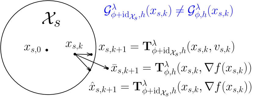
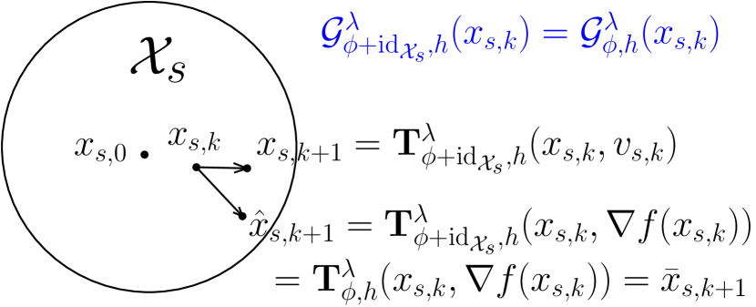
To resolve the mismatch between and , we propose the following probabilistic argument to show that the right-hand-side case of Figure 1 happens in the majority of iterations.
Lemma 3.6.
For any epochs generated by Algorithm 1, define the set and event as
where is an arbitrary positive number. Then it holds that
Proof.
By lemma 3.5, ignoring the squared gradient mapping terms yields
where the last inequality is due to the fact that
for any non-negative random variable and any event . Therefore, conditioning on the event , there exists with and for any . As a result, for any , define . Then given , the triangle inequality and the arithmetic inequality indicate that
| (18) |
Hence we have
| (19) |
Note that the above inequalities hold w.p. 1 conditioning on . Combined with (3.1), we have
Hence we complete the proof. ∎
By Lemma 3.6, we show that epochs never move out of with probability, which indicates that the iterates in these epochs are at least away from the boundary of . In the next lemma, we show that with high probability, the majority of iterates that do not exit will not suffer the mismatch between and .
Lemma 3.7.
For any epochs generated by Algorithm 1, define the set and event as
where is an arbitrary positive number. Then it holds that
Proof.
Theorem 3.8.
Let us set , , and . Suppose the target accuracy satisfies and let be uniformly randomly selected from all iterations that are -away from the corresponding epoch boundary , then there is a high probability event , conditioning on which we have
with , which goes to as The corresponding sample complexity is
Note that the typical complexity for nonconvex stochastic optimization is for finite-sum problem and for general expectation problems. That is, only in the accuracy regime where , utilizing the finite-sum structure will be beneficial. Otherwise, when , it is better to ignore the finite-sum structure and simply treat it as a general expectation. Hence the term in should naturally be close to .
Proof.
First of all, suppose we select and such that both and are upper bounded by . As a result, we have
| (20) |
That is, w.p. at least neither nor happens. Define a third event as
| (21) |
where . That is, by definition, for any , all iterations of epoch- are -close from the epoch starting point . In the meanwhile, the restricted gradient mapping coincides with the real gradient mapping, namely, Therefore, by Lemma 3.5, ignoring the Bregman divergence terms gives
where in (i) is because conditioning on . Suppose we have chosen such that , then and hence
Let us set so that and set , then we have
To maximize the the above probability, we can choose such that
where (i) is due to the choice of and (ii) is due to the choice of and the fact that . Similarly, let us select such that
Now it remains to determine the parameter regimes where the above selection of and satisfies our previous requirements of them. That is, given the current choice of , we require
That is, as long as the target accuracy , then all the previous requirements on and are automatically satisfied. Therefore, combining the previous discussion, we have
Hence we complete the proof. ∎
One comment here is that if one define the event
then . Therefore, it is clear that while could be potentially much closer to 1 than . However, as also includes the points that are close to the epoch boundaries (), whose number is difficult to bound, we analyze the event in Theorem 3.8.
3.2 Improved algorithm for finite-sum setting
Though Algorithm 1 is simple to describe and easy to analyze, it also suffers several drawbacks. In terms of implementation, it is limited to large batch sizes. In addition, when the iterates hit the boundary before the epoch ends, which suggests the set starts to hurdle the algorithm from making progress, Algorithm 1 still continues computing the rest iterations of the epoch, causing a waste of computation. Moreover, in terms of technical analysis of Theorem 3.8, a lot of “good” iterates where are abandoned by the event due to technical difficulties, which makes the final provable success probability to be . In this section we introduce an improved version of Algorithm 1 that both allows arbitrary batch sizes, proper restarting of epochs, and an improved success chance, as described by Algorithm 2.
Compared to Algorithm 1, this variant adopts an additional interpolation step (24) to enable arbitrary batch size. An additional epoch restarting rule was also introduced in Line 6 of Algorithm 2, which enables us to update the “safe region” () for kernel conditioning when it starts to hurdle the optimization progress. We present the convergence results as follows.
Lemma 3.9.
By properly bounding the error term , we obtain Lemma 3.10 for the restricted gradient mapping. The proof of Lemma 3.9 and Lemma 3.10 are both placed in Appendix C.
Lemma 3.10.
For any , set , , and , , then
A significant difference between the Lemma 3.10 and Lemma 3.5 is that in the above result, the actual epoch length are also random variables. Therefore, one may not simply taking average by dividing on both sides. Moreover, intuitively and informally speaking, the output accuracy should be of order . If are too small compared to , then one should frequently restart and take full batch to initialize the epochs, which may cause a bad sample complexity. Therefore, careful probabilistic analyses are required to exclude such undesirable event.
Lemma 3.11.
The proof of this lemma is very similar to that of Lemma 3.6 and 3.7. The only difference is that one needs to pay attention to the relationship . Hence we omit the proof. Next, we provide the final complexity result. As the bound for requires a significantly different analysis, the proof of this theorem is remained in the main paper.
Theorem 3.12.
For any constant batch size , let us set the epoch length as , stepsize , interpolation coefficient , and total epoch number . Suppose the target accuracy satisfies and let be uniformly randomly selected from all iterations, then there is a high probability event such that
In particular, goes to as Suppose we take the batch size , , then the total number of samples consumed is .
Compared to Theorem 3.8, the success probability of the event increases from to . In addition, it also allows a much more flexible selection of batch size and epoch length without additional cost.
Proof.
By lemma 3.10, ignoring the squared gradient mapping terms yields
By expanding the expectation over all possible and , we have for all that
Note that for , since while , we have Repeating the analysis of (18) and (19) yields , which always holds true. Then substituting this lower bound to (3.2) gives
| (26) |
Let us inherit the definition of events and from the proof of Theorem 3.8 while modifying the definition of to . Then we have
Note that for any positive numbers , the arithmetic-harmonic inequality states that
Applying this inequality gives
which implies that
Substituting this bound to the above inequality for and setting yields
where (i) is due to (26) and the fact that
| (29) |
(ii) is due to Lemma 3.11, and :
and (iii) is because we require such that
Therefore, to maximize the above probability, we can choose such that
where the last inequality is due to the fact that Combining all the above discussion, we can conclude that
when taking and Note that the requirement on further implies that and , and hence . Similar to the analysis of Theorem 3.8, by ignoring the Bregman divergence terms of Lemma 3.10, we obtain
Conditioning on , regardless of the random sets and , we have
where the second last inequality is because , and the last inequality is because since we require . As a result,
where the last equality is due to the definition of , , and the fact that coincides with in . As a result, we have
Given the choice of , , , and the fact that , the total sample complexity will be
which indicates an sample complexity for all (or equivalently, ). If larger batch size with is taken, then we obtain an complexity. ∎
3.3 Variance reduced algorithm for general expectation setting
In this section, we discuss how the previously introduced techniques can handle problem (1) with For this setting, we assume the following assumptions.
Assumption 3.13.
For almost every , the function is -smooth relative to the kernel for some random variable . The second moment of exists and we denote .
Besides the above variant of smooth-adaptability assumption for the general expectation setting, we also adopt the following assumption on the variance of the stochastic gradient estimator.
Assumption 3.14.
There exists a function such that for any , we have
Unlike most existing results that require the stochastic gradient variance to be an absolute constant, see e.g. [9], we only require it to be bounded by some function . This assumption strictly includes the bounded variance assumption by setting to be a constant function, but it also allows the variance to go to as grows unbounded, which is important for the considered problem class. A naive example is with . This is a cubic polynomial function whose gradient is quadratic and is hence not Lipschitz continuous. One can explicitly compute that
which indicates that Assumption 3.14 holds with . It is worth noting that there are also different alternative assumptions to capture the potentially unbounded variance. For example, the affine variance assumption introduced in [15]. However, for simplicity, we only discuss the result under current assumption, which more general than the affine variance assumption.
In terms of the algorithm design, it suffices to modify the construction of in Algorithm 2 as
| (31) |
where is a batch of i.i.d. samples from the distribution of . Similarly, the set in (12) are also i.i.d. samples of . After this modification, the Lemma 3.9 still holds true. To avoid repetition, we will only present the main results in this section while moving all the proof to Appendix D.
Theorem 3.15.
Let be some positive constant, for any constant batch size for and with , let us set the epoch length as , stepsize , interpolation coefficient , and total epoch number . Suppose the target accuracy satisfies and let be uniformly randomly selected from all iterations, then there is a high probability event s.t.
Note that if , then the batch size . Consequently, we can compute the total number of samples used as In particular, under the bounded variance assumption adopted in [9] where is a constant, one would expect a significantly smaller sample consumption if grows large.
4 Establishing convergence under the new gradient mapping
In Section 3, we have shown how a simple epoch bounding mechanism and a novel probabilistic argument can activate the kernel conditioning regularity and hence enable the general variance reduction techniques. However, these analyses are all based on the existing Bregman proximal gradient mapping . Consider the special case where , as discussed in Section 2, having a small does not necessarily indicate the near-stationarity of the solution. The existing approaches circumvent this issue by assuming the level set to be compact and hence one may replace the in (10) by , resulting in an convergence in . However, without the compactness assumption of the level set, such an argument may no longer holds. In fact, in the worst-case situation described by Example 2, does not even indicate . Therefore, it is also meaningful to study the convergence under the new Bregman proximal gradient mapping , without relying on the level set compactness.
4.1 An ODE view on deterministic Bregman proximal gradient method
Let us start with the deterministic setting. To establish the convergence of without compact level set assumption, the key is to provide a tight bound on iterations before finding an -stationary point. Let be the iteration sequence of some Bregman proximal gradient type method and let be the first time an -stationary point is obtained, then we aim to provide an that only depends on , , (and ) such that In other words, as long as the algorithm does not find an -stationary point, it will not exit the compact region , which further indicates an iteration complexity. To get a sense on the magnitude of , we start by considering a simple ODE continuation of the Bregman proximal gradient method for differentiable objective functions where . In this case, the limiting Bregman proximal gradient mapping has a simple explicit form.
Lemma 4.1 (Limiting gradient mapping).
Let be twice continuously differentiable and -strongly convex for some , and suppose the Hessian is locally Lipschitz continuous everywhere. Suppose . Then for , the following limit exists
Therefore, we can define the limiting Bregman proximal gradient mapping as
| (32) |
Proof.
Let us inherit the notation from Lemma 2.6 with . By the -strong convexity of , setting in (9) gives
| (33) |
That is, . Note that is locally Lipschitz continuous, there exists some s.t. for all , and is -Lipsthiz continuous in . Denote
as the residual term, then and Consequently,
where the last inequality is due to (33). Taking the limit of proves the first inequality of the lemma. Next, replacing with and utilizing the definition of proves (32). ∎
Based on this Lemma, we construct the following ODE, which is a continuation model of the of Bregman proximal gradient method that takes infinitesimal step sizes:
| (34) |
Suppose Assumption 2.4 holds, then we have the following proposition.
Proposition 4.2.
Proof.
By (32), the ODE (34) reduces to . By definition, we have
On the other hand, we also have
Combining the above two inequalities yields
As when , we have for . The above inequality further implies
where the last inequality is due to (Assumption 2.4). Integrating the above inequality from to yields
Substituting to the above inequality proves the lemma. ∎
Given this proposition, as long as the smooth-adaptable function satisfies the kernel conditioning regularity, the ode (34) (continuized Bregman proximal gradient method) can find an -stationary point of the problem within an distance from the initial point regardless of the potential unboundedness of the level set. On the other hand, from (2) of Example 1, there is an instance for which any non-local-max -stationary points are at least away from the initial point, proving the tightness of the upper bound . Therefore, the intuition behind Proposition 4.2 is that, if the step sizes of the Bregman proximal gradient method are properly selected so that the iterations can sufficiently approximate the ODE solution curve, then we can claim that an -stationary point can be obtained within a provably compact region .
4.2 An adaptive step size control for Bregman proximal gradient method
In this section, we extend the discussion of Section 4.1 to the general case, where can be a convex but non-differentiable function. A simple mechanism is proposed to adaptively determine the step sizes that can properly approximate the ODE (34) without being too conservative:
| (35) |
where is introduced by Assumption 2.1, and are introduced by the Assumption 2.4, and comes from the following bounded subgradient assumption on the non-differentiable term .
Assumption 4.3.
There exists a constant such that for any .
In particular, if , then , the step size rule reduces to . Under this assumption, the adaptively selected step size (35) satisfies the following descent result.
Lemma 4.4.
Proof.
First of all, with , (9) indicates that
| (36) |
where and it satisfies . As result, we complete the proof of Next, let us establish the descent results of this lemma. By standard analysis, we have
where the second inequality is due to . By [33, Theorem 2.1.5, Eq.(2.1.10)], we also have
| (38) |
A Similar inequality also holds for . Suppose , then this situation may only happen if s.t. . In this situation, with , the second row of (4.2) and (38) indicate that
where the last inequality is due to the fact that . Because and , we have and
Consequently, we have
If , the second row of (4.2) and (38) indicate that
Therefore, no matter which value takes, it will at least achieve the minimum descent among the two cases. Hence we complete proof of the lemma. ∎
As a result, we can obtain the following counterpart of Proposition 4.2.
Lemma 4.5.
In particular, when and , the traveling upper bound only suffers a constant overhead comparing to the in Proposition 4.2. Therefore, one does not really need to take an infinitesimal step size to control the searching area.
Proof.
First of all, our requirement on the target accuracy indicates that . Then the second inequality of Lemma 4.4 indicates that
| (39) |
Combined with the first inequality of Lemma 4.4, we have
where the last inequality is due to Assumption 2.4 and (Lemma 4.4). This proves the first part of the lemma. Next, we show the bound on the maximum movement before finding an -stationary solution. By the definition of , we have for . As a result
Applying triangle inequality to the above bound proves the rest of the lemma. ∎
Theorem 4.6.
As a remark, for the polynomial kernel where and are , the maximal iterations before finding an -stationary point is reduced to .
Proof.
By Lemma 4.4 and 4.5, it is straightforward that . Hence, for . Substituting this upper bound to (39) and then summing the resulting inequalities up for yields
which proves the first inequality of the theorem. Note that by Lemma 4.4, our adaptive step size control strategy guarantees that , then the second inequality of the theorem directly follows Lemma 2.8 and the fact that . For the differentiable case where , the result directly follows the definition of and the fact that for any . ∎
As commented in the theorem, the constant with potentially depends . For example, for a degree- polynomial kernel and suppose the level set is unbounded, the worst-case pessimistic estimation gives , which, by Theorem 4.6, suggests that . Such an iteration complexity for making is significantly larger than the complexity for making . Therefore, it is crucial to verify whether the complexity is fundamental for Bregman proximal gradient method or it is just a loose technical artifact. Recall the Example 1 where the standard Bregman proximal gradient method is analyzed, if the iterations move along the positive direction of axis, it is not hard to observe that the gradient size is monotonically decreasing in . According to (35) with , if we set , then and the update rule (35) coincides with the standard Bregman proximal gradient method. Then bullet (3) of Example 1 states that , and at least iterations are needed to find an -stationary point. Therefore, the potential -dependence in provided by Theorem 4.6 is a tight characterization of the iteration complexity.
4.3 Adaptive step size control with stochastic variance reduction
Note that the exact gradient norm is required in the adaptive step size control scheme (35), which is inaccessible in the stochastic setting. Moreover, as both and are random variables, the complex interplay between them makes a sheer in-expectation analysis insufficient to bound the sample complexity. Instead, a high probability bound will be favorable in the following discussion. Basically, we will still adopt the framework of Algorithm 2, while removing the bound constraint and the early stop mechanism (Line 6) of each epoch. In other words, we set in Algorithm 2. In addition, we modify the update (24) with the following update under adaptive step size control:
| (40) |
| (41) |
By slightly modifying the analysis of (36) and (C.1), we obtain the following descent result for the update (40) and (41), whose proof is omitted.
Lemma 4.7.
To establish the counterpart of Lemma 4.4, a high probability bound on is required. However, simply applying the standard Azuma-Hoeffding inequality may incur additional dependence on problem dimension. To avoid such a dependence, we need the following large deviation bound for vector-valued martingale in 2-smooth normed spaces from [24].
Definition 4.8.
Let denote a finite-dimensional space equipped with some norm . We say the space (and the norm on ) is -regular for some , if there exists a constant and a norm on such that the function is -smooth and is -compatible with . That is, for , we have
We should notice that the and here has nothing to do with the condition numbers that are widely used throughout the paper.
Theorem 4.9 (Theorem 2.1-(ii), [24]).
Suppose is -regular for some and is an -valued martingale difference sequence w.r.t. the filtration and default . Suppose satisfies the following light-tail property:
When , for any , it holds that
Consider where stands for the standard Euclidean (L-2) norm that we use throughout this paper. Setting and in Definition 4.8, then straight computation shows that is -regular. As a result, we have the following bound for
Lemma 4.10.
Proof.
Fix any epoch index , consider the sequence defined as
In the above definition, the index runs through , and the index can take value from given each . For each in our index range, stands for the -th sample from the batch . Then by direct computation, we have and forms a martingale difference sequence if the index runs in a lexicographical order. Note that
where the last inequality is because , Assumption 2.4, and the fact that
As this bound holds almost surely, we have . Applying Theorem 4.9 to this martingale difference sequence gives
Finally, setting gives , which proves the lemma. ∎
Let us define as the stochastic surrogate of the the exact Bregman proximal gradient mapping , then we have the following lemma.
Lemma 4.11.
Proof.
First of all, by Lemma 4.10, setting gives
| (42) |
Given , we have with probability at least that
Combining the above inequality with Lemma 4.7, we have
This proves the first inequality of the lemma. Next, let us prove the result by discussing the following cases:
case 1. When , regardless of , the second row of (4.3) indicates that
case 2. If and . This case may happen only if , namely, only if Note that for some , in this case, we have . Then the second row of (4.3) gives
case 3. If and . In this case, the third row of (4.3) indicates that
Combining cases 1,2, and 3, we know the least descent among the three cases are guaranteed to be achieved. Note that if , direct computation shows that lower bounds the descents in all three cases, which completes the proof. ∎
Consequently, define as the first time that we find a point , and set as the maximum traveling distance until finding such a point. Then the following theorem holds while the proof is omitted.
Theorem 4.12.
Proof.
The bounds on and are straightforward consequence of Lemma 4.11. We only need to show the bound of exact Bregman proximal gradient mapping. For notational simplicity, let us denote . Then by definition, we have . Let be the ideal intermediate update point that uses the exact gradient , hence the exact gradient mapping will be . By the proof of Lemma 3.2 and (42), we have
Consequently, with , we further obtain that
Using the fact that , we finish the proof of . ∎
5 Comparison and conclusion
Comparison.
After establishing the convergence and complexities of the (deterministic or stochastic variance reduced) Bregman proximal gradient methods under both the old and new gradient mappings, it is crucial to make a thorough comparison between them. For general composite (deterministic or stochastic) nonconvex optimization of form (1), suppose we aim to find some solution such that
| (45) |
either deterministically, in expectation, or with high probability.
In the deterministic setting, the existing results [4, 16, 17, 28, 36, etc.] typically guarantee that . Assuming the level set to be compact and following Remark 2.9, the existing analysis based on the old gradient mapping can provide an iteration complexity of for finding some that satisfies (45), which can be improved to by adopting a similar approach of (10). On the other hand, based on the analysis of the new gradient mapping provided in Section 4, with additional -Lipschitz continuity assumption on the non-differentiable term , it takes iterations to find an that satisfies (45). Because , it always holds that . Comparing the two results, it can be observed that the old analysis is more flexible in terms of the , while being more restrictive in terms of the compactness of the level set . If the level set is not much larger than in the sense that and are having similar magnitudes, then the existing analysis based on the old gradient mapping can provide a comparable iteration complexity as that provided by our Theorem 4.6. However, if is compact but much larger than , then our new analysis will provide a much tighter bound on iteration complexity. If is unbounded so that , then the existing analyses fail.
In the stochastic setting, let us consider the finite-sum case for example. After adopting the epoch bound mechanism and the probabilistic argument in Section 3, we require to obtain some such that in conditional-expectation of some high probability event . Unlike the deterministic case where the iteration sequence provably stays in the level set , the randomness of the algorithm gives a probability of the iteration sequence to move outside . Based on the compactness of , if it one is able to show that is almost surely bounded in some compact set (see e.g. [9, Theorem 19]), then one may set s.t. satisfies (45) with a sample complexity of . If more careful analysis is adopted, an improved complexity of can be possible. If all the “if” arguments in the above discussion are done, and the set (agnostic to users) is not much larger than in sense that and share a similar magnitude, then the complexity provided by the analysis of old gradient mapping can be comparable to that provided by the analysis based on new gradient mapping. However, if is unbounded, then all the analysis based on the old gradient mapping can fail to provide stationarity of the output solutions.
Conclusion and future works.
Several important questions in the Bregman proximal gradient methods for solving nonconvex composite stochastic optimization problems are considered in this paper. We reveal several weaknesses of the current widely adopted Bregman proximal gradient mapping , including the potential inability to capture stationarity for unbounded problems and the sensitivity to the choice of kernel . We resolve this issue by proposing an alternative gradient mapping that is provably comparable with the standard near-stationarity measure . We also propose a new kernel-conditioning regularity assumption that enables us to exploit the variance reduction techniques in the stochastic setting. An improved sample complexity under the old gradient mapping as well as brand-new complexity results and analysis techniques under the new gradient mapping are provided in this paper. In terms of future works, a potential interesting direction could be studying the proper form of kernel-conditioning regularity for smooth-adaptable functions with while being singular on , for which the examples can be found in [30].
Appendix A Supporting Lemmas
Lemma A.1 (Three-Point Property of Tseng [37]).
Let be a convex function, and let be the Bregman distance for . For a given vector , let Then
Lemma A.2 (Lemma 2 finite-sum case of [35]).
Let be generated by (12), suppose and the sampled index are uniformly randomly picked from with replacement, then
where the expectation term of satisfies
In particular, we have slightly modified the second inequality to suit our analysis.
Lemma A.3 (Lemma 2 general expectation case of [35]).
Appendix B Proof of Section 3.1
B.1 Proof of Lemma 3.2
B.2 Proof of Lemma 3.3
B.3 Proof of Lemma 3.5
Appendix C Proof of Section 3.2
C.1 Proof of Lemma 3.9
Proof.
First of all, similar to the proof Lemma 3.3, we have
where (i) is due to the convexity of and the following scaling property
and (ii) is due to Lemma A.1 and the optimality of Notice that by Lemma 3.2, we also have
Multiplying both sides of the above inequality by and add it to (C.1) proves the lemma. ∎
C.2 Proof of Lemma 3.10
Proof.
First, by Lemma A.2, we can bound the expectation of the gradient error term by
Substituting this bound to Lemma 3.9, we have the following descent result throughout the -th epoch
| (50) | ||||
Suppose we choose and we choose . Then we have
Substitute the bound to the previous inequality, summing up over all epochs, and taking the expectation over all randomness proves the lemma. ∎
Appendix D Proof of Section 3.3
In this section we present the analysis for obtaining Theorem 3.15.
D.1 Establishing the square summability of surrogate gradient mapping
Lemma D.1.
For any , set , , , and for some , , then
Proof.
First, let us bound the expectation of the squared gradient error term by
where (i) is by summing up the inequalities of Lemma A.3, (ii) is by Assumption 3.13, 3.14 and the analysis of (C.2). Substituting this bound to Lemma 3.9, selecting for some , and repeating the analyses of (C.2) and (C.2) proves the lemma. ∎
D.2 Bounding the probability of events and
Lemma D.2.
D.3 Proof of Theorem 3.15
Proof.
With the new square summability result in Lemma D.1, mimicking the analysis of (3.2) and (26) by expanding the expectation over all possible and , we have for all that
| (52) |
Let us inherit the definition of events and from the proof of Theorem 3.12. Let us set and repeat the analyses from (3.2) to (3.2), we obtain
where (i) is due to (52) and (29), both (ii) and (iii) are due to setting , , and in Lemma D.2, as well as the choice of , , and the fact that . Given the above parameter selections, straight computation gives , , and Therefore, to maximize the above probability, we can choose such that
Combining all the above discussion, we conclude that
when taking and Note that the requirement on further implies that . When , we also have , and hence . Therefore, repeating the analysis of Theorem 3.12 by ignoring the Bregman divergence terms of Lemma 3.10 yields
Again, conditioning on , we bound by
As a result, repeating the discussion of (3.2) yields
Since coincides with in . We further have
Hence we complete the proof. ∎
Appendix E Proof of Example 1
Proof.
Because (1) is straightforward, we start with proving the argument (2). Note that
By the symmetry of the objective function, let us assume in the following discussion. By , we have , and hence Together with , the second term of satisfies As when , we have
which indicates that
Finally, let us prove (3) of Example 1. To begin with, we show by induction that . By initialization, holds true. Suppose , then . Denote and , then substituting these derivatives to the BPG subproblem yields
| (53) |
In (53), only appears in the last norm polynomial terms. Hence we have . Next, substituting to (53) yields a simplified subproblem only in terms of the variable , whose KKT condition can be written as
| (54) |
Since for . With , the KKT condition (54) indicates that is monotonically increasing. Hence, substituting the value of , we have
Take the -th root and apply the inequality that , we obtain
| (55) |
where the last inequality is because . Now, we are ready to derive the upper bound for . Define , for , where . Then we know . On the other hand, (55) indicates that . Therefore, we have
That is, . Notice that if we want , then we will need
and hence we have Substituting this bound and to the gradient yields
Hence we complete the proof. ∎
References
- [1] Yossi Arjevani, Yair Carmon, John C Duchi, Dylan J Foster, Nathan Srebro, and Blake Woodworth. Lower bounds for non-convex stochastic optimization. Mathematical Programming, 199(1-2):165–214, 2023.
- [2] Heinz H Bauschke, Jérôme Bolte, and Marc Teboulle. A descent lemma beyond lipschitz gradient continuity: first-order methods revisited and applications. Mathematics of Operations Research, 42(2):330–348, 2017.
- [3] Amir Beck. First-order methods in optimization. SIAM, 2017.
- [4] Jérôme Bolte, Shoham Sabach, Marc Teboulle, and Yakov Vaisbourd. First order methods beyond convexity and lipschitz gradient continuity with applications to quadratic inverse problems. SIAM Journal on Optimization, 28(3):2131–2151, 2018.
- [5] Alejandro Carderera, Mathieu Besançon, and Sebastian Pokutta. Simple steps are all you need: Frank-wolfe and generalized self-concordant functions. Advances in Neural Information Processing Systems, 34, 2021.
- [6] Yair Carmon, John C Duchi, Oliver Hinder, and Aaron Sidford. Lower bounds for finding stationary points ii: first-order methods. Mathematical Programming, 185(1-2):315–355, 2021.
- [7] Ashok Cutkosky and Francesco Orabona. Momentum-based variance reduction in non-convex sgd. Advances in neural information processing systems, 32, 2019.
- [8] Damek Davis, Dmitriy Drusvyatskiy, and Kellie J MacPhee. Stochastic model-based minimization under high-order growth. arXiv preprint arXiv:1807.00255, 2018.
- [9] Kuangyu Ding, Jingyang Li, and Kim-Chuan Toh. Nonconvex stochastic bregman proximal gradient method with application to deep learning. arXiv preprint arXiv:2306.14522, 2023.
- [10] Radu Alexandru Dragomir, Mathieu Even, and Hadrien Hendrikx. Fast stochastic bregman gradient methods: Sharp analysis and variance reduction. In International Conference on Machine Learning, pages 2815–2825. PMLR, 2021.
- [11] Radu-Alexandru Dragomir, Adrien B Taylor, Alexandre d’Aspremont, and Jérôme Bolte. Optimal complexity and certification of bregman first-order methods. Mathematical Programming, pages 1–43, 2021.
- [12] Dmitriy Drusvyatskiy and Adrian S Lewis. Error bounds, quadratic growth, and linear convergence of proximal methods. Mathematics of Operations Research, 43(3):919–948, 2018.
- [13] Pavel Dvurechensky, Kamil Safin, Shimrit Shtern, and Mathias Staudigl. Generalized self-concordant analysis of frank–wolfe algorithms. Mathematical Programming, pages 1–69, 2022.
- [14] Cong Fang, Chris Junchi Li, Zhouchen Lin, and Tong Zhang. Spider: Near-optimal non-convex optimization via stochastic path-integrated differential estimator. Advances in neural information processing systems, 31, 2018.
- [15] Matthew Faw, Isidoros Tziotis, Constantine Caramanis, Aryan Mokhtari, Sanjay Shakkottai, and Rachel Ward. The power of adaptivity in sgd: Self-tuning step sizes with unbounded gradients and affine variance. In Conference on Learning Theory, pages 313–355. PMLR, 2022.
- [16] Tianxiang Gao, Songtao Lu, Jia Liu, and Chris Chu. Randomized bregman coordinate descent methods for non-lipschitz optimization. arXiv preprint arXiv:2001.05202, 2020.
- [17] Tianxiang Gao, Songtao Lu, Jia Liu, and Chris Chu. On the convergence of randomized bregman coordinate descent for non-lipschitz composite problems. In ICASSP 2021-2021 IEEE International Conference on Acoustics, Speech and Signal Processing (ICASSP), pages 5549–5553. IEEE, 2021.
- [18] Benjamin Grimmer. Radial subgradient method. SIAM Journal on Optimization, 28(1):459–469, 2018.
- [19] Benjamin Grimmer. Radial duality part ii: applications and algorithms. Mathematical Programming, pages 1–37, 2023.
- [20] Filip Hanzely and Peter Richtárik. Fastest rates for stochastic mirror descent methods. Computational Optimization and Applications, 79:717–766, 2021.
- [21] Filip Hanzely, Peter Richtarik, and Lin Xiao. Accelerated bregman proximal gradient methods for relatively smooth convex optimization. Computational Optimization and Applications, 79:405–440, 2021.
- [22] Mingyi Hong, Siliang Zeng, Junyu Zhang, and Haoran Sun. On the divergence of decentralized nonconvex optimization. SIAM Journal on Optimization, 32(4):2879–2908, 2022.
- [23] Rie Johnson and Tong Zhang. Accelerating stochastic gradient descent using predictive variance reduction. Advances in neural information processing systems, 26, 2013.
- [24] Anatoli Juditsky and Arkadii S Nemirovski. Large deviations of vector-valued martingales in 2-smooth normed spaces. arXiv preprint arXiv:0809.0813, 2008.
- [25] A. Ya. Kruger. On fréchet subdifferentials. Journal of Mathematical Sciences, 116:3325–3358, 2003.
- [26] Puya Latafat, Andreas Themelis, Masoud Ahookhosh, and Panagiotis Patrinos. Bregman finito/miso for nonconvex regularized finite sum minimization without lipschitz gradient continuity. SIAM Journal on Optimization, 32(3):2230–2262, 2022.
- [27] Khanh Hien Le Thi, Nicolas Gillis, and Panagiotis Patrinos. Inertial block mirror descent method for non-convex non-smooth optimization.
- [28] Qiuwei Li, Zhihui Zhu, Gongguo Tang, and Michael B Wakin. Provable bregman-divergence based methods for nonconvex and non-lipschitz problems. arXiv preprint arXiv:1904.09712, 2019.
- [29] Haihao Lu. “relative continuity” for non-lipschitz nonsmooth convex optimization using stochastic (or deterministic) mirror descent. INFORMS Journal on Optimization, 1(4):288–303, 2019.
- [30] Haihao Lu, Robert M Freund, and Yurii Nesterov. Relatively smooth convex optimization by first-order methods, and applications. SIAM Journal on Optimization, 28(1):333–354, 2018.
- [31] Mahesh Chandra Mukkamala, Peter Ochs, Thomas Pock, and Shoham Sabach. Convex-concave backtracking for inertial bregman proximal gradient algorithms in nonconvex optimization. SIAM Journal on Mathematics of Data Science, 2(3):658–682, 2020.
- [32] Mahesh Chandra Mukkamala, Felix Westerkamp, Emanuel Laude, Daniel Cremers, and Peter Ochs. Bregman proximal framework for deep linear neural networks. arXiv preprint arXiv:1910.03638, 2019.
- [33] Yurii Nesterov et al. Lectures on convex optimization, volume 137. Springer, 2018.
- [34] Lam M Nguyen, Marten van Dijk, Dzung T Phan, Phuong Ha Nguyen, Tsui-Wei Weng, and Jayant R Kalagnanam. Finite-sum smooth optimization with sarah. Computational Optimization and Applications, 82(3):561–593, 2022.
- [35] Nhan H Pham, Lam M Nguyen, Dzung T Phan, and Quoc Tran-Dinh. Proxsarah: An efficient algorithmic framework for stochastic composite nonconvex optimization. The Journal of Machine Learning Research, 21(1):4455–4502, 2020.
- [36] Marc Teboulle. A simplified view of first order methods for optimization. Mathematical Programming, 170(1):67–96, 2018.
- [37] Paul Tseng. On accelerated proximal gradient methods for convex-concave optimization. submitted to SIAM Journal on Optimization, 2(3), 2008.
- [38] Zhe Wang, Kaiyi Ji, Yi Zhou, Yingbin Liang, and Vahid Tarokh. Spiderboost: A class of faster variance-reduced algorithms for nonconvex optimization. arXiv, 2018, 2018.
- [39] Junyu Zhang and Mingyi Hong. First-order algorithms without lipschitz gradient: A sequential local optimization approach. arXiv preprint arXiv:2010.03194, 2020.
- [40] Renbo Zhao and Robert M Freund. Analysis of the frank-wolfe method for logarithmically-homogeneous barriers, with an extension. arXiv e-prints, pages arXiv–2010, 2020.
- [41] Dongruo Zhou and Quanquan Gu. Lower bounds for smooth nonconvex finite-sum optimization. In International Conference on Machine Learning, pages 7574–7583. PMLR, 2019.