Convergence Analysis of Non-Strongly-Monotone Stochastic Quasi-Variational Inequalities

Abstract

While Variational Inequality (VI) is a well-established mathematical framework that subsumes Nash equilibrium and saddle-point problems, less is known about its extension, Quasi-Variational Inequalities (QVI). QVI allows for cases where the constraint set changes as the decision variable varies allowing for a more versatile setting. In this paper, we propose extra-gradient and gradient-based methods for solving a class of monotone Stochastic Quasi-Variational Inequalities (SQVI) and establish a rigorous convergence rate analysis for these methods. Our approach not only advances the theoretical understanding of SQVI but also demonstrates its practical applicability. Specifically, we highlight its effectiveness in reformulating and solving problems such as generalized Nash Equilibrium, bilevel optimization, and saddle-point problems with coupling constraints.

1 Introduction

Variational Inequality (VI) problems find applications in various areas like convex Nash games, traffic equilibrium, and economic equilibrium [9]. The Stochastic Variational Inequality (SVI) extends VI theory to address decision-making problems involving uncertainty [11]. An extension of VI, known as Quasi-Variational Inequality (QVI) emerges when the constraint set depends on the decision variable. From the Nash equilibrium game perspective, QVI captures interdependencies among players’ strategy sets, particularly in scenarios involving shared resources.

In this paper, we consider a Stochastic QVI (SQVI) problem. In particular, the goal is to find $x^{*}\in K(x^{*})$ such that

$$\langle F(x^{*}),y-x^{*}\rangle\geq 0,\quad\forall y\in K(x^{*}),$$ (SQVI)

where $K:X\to 2^{X}$ is a set-valued mapping with non-empty, closed and convex values such that $K(x)\subseteq X$ for all $x\in X$, $X\subseteq\mathbb{R}^{n}$ is a convex and compact set, $F(x)\triangleq\mathbb{E}[G(x,\xi)]$, $\xi:\Omega\to\mathbb{R}^{d}$, ${G}:X\times\mathbb{R}^{d}\rightarrow\mathbb{R}^{n}$, and the associated probability space is denoted by $(\Omega,{\cal F},\mathbb{P})$.

Although the theoretical results and algorithm development for VIs are rich and fruitful [1, 14, 16, 25, 37, 26, 19, 21], research studies on QVIs remain limited and most of the existing methods for solving VIs are not amendable for solving (SQVI) which calls for the development of new techniques and iterative methods. In particular, the primary focus of existing research studies for QVIs is on solution existence [32] and the development of algorithms often requires restrictive assumptions such as strong monotonicity [23]. To fill this gap, in this paper, we aim to develop efficient inexact iterative methods for solving (SQVI) under less restrictive assumptions with convergence rate guarantees. In the deterministic setting, several studies have explored numerical approaches for solving QVIs [31, 3, 8, 22, 28, 33, 34, 29]. Notably, [23] demonstrated a linear convergence rate for the strongly monotone QVI problem (see also [27]). In the stochastic regime, in our previous work [2], we obtained a linear convergence rate under strong monotonicity assumptions. In this paper, we extend the result to monotone SQVIs, where the operator $F$ satisfies the quadratic growth property (see Definition 1).

1.1 Outline of the Paper

In the next section, we explore how the SQVI problem fits into well-known problems in optimization and game theory. In Section 3, we outline the key contributions of our work. Then, in Section 4, we lay out the key assumptions needed for our convergence analysis. Section 5 introduces inexact extra-gradient and gradient-based algorithms, and in Section 6, we show the effectiveness of the proposed methods in solving real-world examples. In Section 7, we summarize our key findings and propose directions for future research.

2 Applications

2.1 Generalized Nash Equilibruim

Nash equilibrium (NE) is a fundamental concept in game theory where a finite collection of selfish agents compete with each other and seek to optimize their own individual objectives. An NE is described as a collection of specific strategies chosen by all the players, where no player can reduce their cost by unilaterally changing their strategy within their feasible strategy set. The Generalized Nash equilibrium Problem (GNEP) is an extension of the classic NE Problem (NEP), in which players interact also at the level of the feasible sets, i.e., each player’s strategy set depends on other players’ strategies. This situation arises naturally if the players share some common resource, e.g., a communication link, an electrical transmission line, etc. GNEP has been extensively utilized in the literature to formulate applications arising in economics, operations research, and other fields [7, 17]. Consider $N$ players each with cost function $f_{i}(x_{i},x_{(-i)})\triangleq\mathbb{E}[h(x_{i},x_{(-i)},\xi)]$ for $i=1\ldots,N$, where $x_{i}$ is the strategy of player $i$ and $x_{(-i)}$ is the strategy of other players. Each player $i$’s objective is to solve the following optimization problem:

$$\min_{x_{i}}f_{i}(x_{i},x_{(-i)})\quad\hbox{s.t.}\quad x_{i}\in K_{i}(x_{(-i)}),$$

where $K_{i}(x_{(-i)})=\{x_{i}\in\mathbb{R}^{n_{i}}|g_{i}(x_{i},x_{(-i)})\leq 0\}$ is a closed convex set-valued map. $f_{i},g_{i}:\mathbb{R}^{n}\times\mathbb{R}^{m}\to\mathbb{R}$ are continuously differentiable. By defining $K(x)=\prod_{i=1}^{N}K_{i}(x_{(-i)})$ and $F(x)=[\nabla_{x_{i}}f_{i}(x)]_{i=1}^{N}$, finding a GNE will be equivalent to solving the following SQVI problem. $\langle F(x^{*}),x-x^{*}\rangle\geq 0,$ for all $x\in K(x^{*})$.

2.2 Bilevel Optimization

A bilevel optimization problem is hierarchical decision-making where one optimization problem is nested within another. This problem has a variety of applications, including data hyper cleaning, hyper-parameter optimization, and meta-learning in machine learning [18, 10]. This problem can be formulated as follows:

$$\min_{u\in U}~{}f(u,w(u))\quad\hbox{s.t.}\quad w(u)\in\mathop{\rm argmin}_{w\in W}~{}g(u,w),$$ (1)

where $f(u,w)\triangleq\mathbb{E}[h(u,w,\xi)]$, $f,g:\mathbb{R}^{n}\times\mathbb{R}^{m}\to\mathbb{R}$ are continuously differentiable, $U\subseteq\mathbb{R}^{n}$ and $W\subseteq\mathbb{R}^{m}$ are convex and compact sets. This problem can be equivalently represented as the following minimization problem:

$$\min_{u\in U,w\in W}~{}f(u,w)\quad\hbox{s.t.}\quad w\in S(u),$$ (2)

where $S(u)$ is the solution to the lower-level problem in (1) for any given $u\in U$. Note that (2) in its general form can be NP-hard, therefore, it is imperative to seek a first-order stationary solution, i.e., finding $(u^{*},w^{*})$ such that $\langle\nabla_{u}f(u^{*},w^{*}),u-u^{*}\rangle+\langle\nabla_{w}f(u^{*},w^{*}),w-w^{*}\rangle\geq 0$ for any $u\in U$ and $w\in S(u^{*})$, which is a special case of (SQVI) by defining $x\triangleq[u^{\top},w^{\top}]^{\top}$, $F(x)\triangleq[\nabla_{u}f(u,w),\nabla_{w}f(u,w)]^{\top}$, and $K(x)\triangleq U\times S(u)$.

2.3 Saddle Point Problems with Coupling Constraints

Recently, minimax optimization problems, i.e., $\min_{u\in U}\max_{w\in W}f(u,w)$, have received considerable attention due to their relevance to a wide range of machine learning (ML) problems such as reinforcement learning, generative adversarial networks (GAN), fairness in machine learning, and generative adversarial imitation learning. Convex-concave minimax problems can be also viewed from a game theory perspective in which the objective function severs as a payoff function and one player aims to minimize the payoff while the second player’s goal is to maximize it. In this context, a saddle point solution $(u^{*},w^{*})$ serves as both a minimum of $f$ in the $u$-direction and a maximum of $f$ in the $w$-direction. Here, $w^{*}$ represents the inner player’s best response to their opponent’s strategy $u^{*}$, and a saddle point $(u^{*},w^{*})$ is also called a Nash equilibrium (NE).

Here, we consider a more general SP problem where the constraint depends on the decisions of both players, i.e.,

$$\min_{u\in U}\max_{w\in W}f(u,w)\quad\hbox{s.t.}\quad g(u,w)\leq 0,$$ (3)

where $f(u,w)\triangleq\mathbb{E}[h(u,w,\xi)]$, $U$ and $W$ are convex sets. Such problems have numerous applications in various fields such as adversarial attacks in network flow problems [36]. Because of the dependency of the constraint on both variables, if $g$ is not jointly convex in both $x$ and $y$ then this problem cannot be formulated as traditional VI but we can reformulate it as QVI. From the first order optimality condition of (3), we have that

$$\langle\nabla_{x}f(u^{*},w^{*}),u-u^{*}\rangle\geq 0,\forall u\in\{u\in U\mid g(u,w^{*})\leq 0\}$$

$$\langle\nabla_{w}f(u^{*},w^{*}),w^{*}-w\rangle\geq 0,\forall w\in\{w\in W|g(u^{*},w)\leq 0\}.$$

Defining $F(x^{*})=\begin{bmatrix}\nabla_{u}f(x^{*})\\ -\nabla_{\color[rgb]{0,0,0}w}f(x^{*})\end{bmatrix}$ and $K(x^{*})\triangleq U(w^{*})\times W(u^{*})$, solving (3) will be equivalent to solving the following SQVI problem. $\langle F(x^{*}),x-x^{*}\rangle\geq 0,\forall x\in K(x^{*})$.

3 Contributions

Motivated by the absence of efficient methods to solve non-strongly monotone SQVI problems, we develop extra-gradient and gradient-based schemes to solve a class of monotone SQVI where the operator satisfies quadratic growth property. In particular, we examine the convergence rate of the proposed method when computing the projection onto the constraint may be challenging. In cases where this projection is not easily computed, during each iteration of the proposed method, the projection step is solved inexactly, and we analyze the impact of the associated error on the convergence rate. By improving the accuracy of such approximations at a suitable rate, combined with a variance reduction technique, we demonstrate a linear convergence rate in terms of the outer iterations. Furthermore, we show an oracle complexity of $\mathcal{O}(1/\epsilon^{2})$; that is, to achieve an $\epsilon$-solution, $\mathcal{O}(1/\epsilon^{2})$ sample operators need to be computed. The oracle complexity will improve to $\mathcal{O}(\log(1/\epsilon))$ for the deterministic case. To the best of our knowledge, our proposed algorithms are the first with a convergence rate guarantee to solve non-strongly monotone SQVIs.

4 Preliminaries

In this section, first, we define important notations and then we present the definitions, assumptions, and essential technical lemmas required for our convergence analysis.

4.1 Notations

Throughout the paper, $\|x\|$ denotes the Euclidean vector norm, i.e., $\|x\|=\sqrt{x^{T}x}$. $\mathcal{P}_{K}[x]$ is the projection of $x$ onto the set $K$, i.e. $\mathcal{P}_{K}[x]=\mbox{argmin}_{y\in K}\|y-x\|$. $\mathbb{E}[x]$ is used to denote the expectation of a random variable $x$. We let $X^{*}$ denote the set of optimal solution of (SQVI) problem, which is assumed to be nonempty.

4.2 Assumptions and Technical Lemmas

In this paper, we consider a monotone operator $F$ that has a quadratic growth property, which is defined next.

Definition 1.

An operator $F$ has a quadratic growth (QG) property on set $X$ if there exists a constant ${\color[rgb]{0,0,0}\mu_{F}}>0$ such that for any $x\in X$ and $y=\mathcal{P}_{X^{*}}(x)$

$$\langle F(x)-F(y),x-y\rangle\geq{\color[rgb]{0,0,0}\mu_{F}}\|x-y\|^{2},\quad\forall x\in X.$$

It is worth noting that, unlike the strong monotonicity assumption, the QG property does not imply a unique solution. In fact, QG property is a weaker assumption than strong monotonicity [24]. As an example of a QG operator, consider function $f(x)\triangleq g(Ax)+c^{T}x$, where $g$ is a smooth and strongly convex function, $A\in\mathbb{R}^{n\times m}$ is a nonzero general matrix and $c\in\mathbb{R}^{n}$. One can show that $\nabla f(x)$ satisfies the QG property [24] while $\nabla f(x)$ may not be strongly monotone unless $A$ has a full column rank.

Next, we state our main assumptions considered in the paper.

Assumption 1.

(i) The set of optimal solution, $X^{*}$ is nonempty. (ii) Operator $F:X\rightarrow\mathbb{R}^{n}$ is monotone, i.e., $\langle F(x)-F(y),x-y\rangle\geq 0$ for all $x,y\in X$, and satisfies the QG property. (iii) $F$ is $L$-Lipschitz continuous on $X$, i.e.,

$$\|F(x)-F(y)\|\leq L\|x-y\|,\quad\forall x,y\in X.$$

If $\mathcal{F}_{k}$ denotes the information history at epoch $k$, then we have the following requirements on the associated filtrations where $\bar{w}_{k,N_{k}}\triangleq\tfrac{1}{N_{k}}{\sum_{j=1}^{N_{k}}{\color[rgb]{0,0,0}(G(x_{k},\xi_{j,k})-F(x_{k}))}}$.

Assumption 2.

There exists $\nu>0$ such that $\mathbb{E}[\bar{w}_{k,N_{k}}\mid\mathcal{F}_{k}]=0$ and $\mathbb{E}[\|\bar{w}_{k,N_{k}}\|^{2}\mid\mathcal{F}_{k}]\leq\tfrac{\nu^{2}}{N_{k}}$ holds almost surely for all $k$, where $\mathcal{F}_{k}\triangleq\sigma\{x_{0},x_{1},\ldots,x_{k-1}\}$.

In our analysis, the following technical lemma for projection mappings is used.

Lemma 1.

[5] Let $X\subseteq\mathbb{R}^{n}$ be a nonempty closed and convex set. Then the following hold: (a) $\|\mathcal{P}_{X}[u]-\mathcal{P}_{X}[v]\|\leq\|u-v\|$ for all $u,v\in\mathbb{R}^{n}$; (b) $(\mathcal{P}_{X}[u]-u)^{T}(x-\mathcal{P}_{X}[u])\geq 0$ for all $u\in\mathbb{R}^{n}$ and $x\in X$.

Gap Function. Now, we define a gap function to measure the quality of the solution obtained from the algorithm. In particular, for a given iterate $x$ we use $\text{dist}(x,X^{*})\triangleq\|x-\mathcal{P}_{X^{*}}(x)\|$ to find the distance of the solution obtained by the algorithm from the optimal solution set $X^{*}$. Moreover, we call $x$ to be an $\epsilon$-solution if $\|x-\bar{x}\|\leq\epsilon$ where $\bar{x}\triangleq\mathcal{P}_{X^{*}}(x)$.

5 Proposed Method

A popular method for solving SVI problems is the stochastic Extra-gradient (SEG) method originally proposed by Korpelevic [16] for deterministic setting. In particular, when $K(x)=K$ is a closed and convex set, the (SQVI) problem reduces to SVI. In each iteration of SEG, two consecutive projection steps are calculated with the following updates:

$$u_{k}\leftarrow\mathcal{P}_{K}\left(x_{k}-\eta\frac{\sum_{j=1}^{N_{k}}G(x_{k},\xi_{j,k})}{N_{k}}\right);$$

$$x_{k+1}\leftarrow\mathcal{P}_{K}\left(u_{k}-\eta\frac{\sum_{j=1}^{N_{k}}G(u_{k},\xi_{j,k})}{N_{k}}\right);$$

The challenge in developing algorithms for solving SQVI primarily arises from the dynamic nature of the constraint set, which evolves during iterations. To manage this variation, it is crucial to ensure that the set $K(x)$ does not change drastically as $x$ varies. To achieve this, we impose a condition on the corresponding projection operator, which guarantees that the projection remains contractive with respect to the set $K(x)$. This condition is formally stated in the following assumption. Note that this is a common assumption for the convergence guarantee of QVI problems (see [30]).

Assumption 3.

There exists $\gamma>0$ such that $\|\mathbf{P}_{K(x)}[u]-\mathbf{P}_{K(y)}[u]\|\leq\gamma\|x-y\|$ for all $x,y,u\in X$ and $\gamma+\sqrt{1-{\mu_{F}}^{2}/L^{2}}<1$.

Furthermore, from an algorithmic perspective to ensure convergence guarantee due to changes in the constraint set, one approach is to introduce a retraction step [23], denoted as $(1-\alpha)x_{k}+\alpha u_{k}$ for some $\alpha\in[0,1]$. By integrating these ideas, we present the following variant of the SEG method for solving (SQVI).

$$v_{k}\leftarrow\mathcal{P}_{K(x_{k})}\left(x_{k}-\eta\frac{\sum_{j=1}^{N_{k}}G(x_{k},\xi_{j,k})}{N_{k}}\right);$$

$$u_{k}\leftarrow(1-b_{k})x_{k}+b_{k}v_{k}$$

$$y_{k}\leftarrow\mathcal{P}_{K(u_{k})}\left(u_{k}-\eta\frac{\sum_{j=1}^{N_{k}}G(u_{k},\xi_{j,k})}{N_{k}}\right);$$

$$x_{k+1}\leftarrow(1-\alpha_{k})x_{k}+\alpha_{k}y_{k};$$

It is worth noting that, the exact computation of the projection onto the constraint set can be computationally expensive or even infeasible in certain scenarios. To overcome this limitation, we propose utilizing approximation techniques, allowing us to obtain practical solutions even when precise projections are unattainable. In particular, we assume that the constraints are comprised of the nonlinear smooth function $g:X\times X\to\mathbb{R}^{m}$, i.e., $K(x)=\{y\in X\mid g(x,y)\leq 0\}$, such that $g(x,\cdot)$ is convex for any $x\in X$. To handle the nonlinear constraints, in Algorithm 1, we introduce an inexact Extra-gradient SQVI (iEG-SQVI) method. In this method, at each step of the algorithm, we approximately solve the projection using an inner algorithm denoted as $\mathcal{M}$, which operates for a specified number of inner iterations, denoted as $t_{k}$. To guarantee fast convergence, Algorithm $\mathcal{M}$ should satisfy the following property.

Assumption 4.

For any $x\in\mathbb{R}^{n}$, any closed and convex set $K\subseteq\mathbb{R}^{n}$, and an initial point $u_{0}$, $\mathcal{M}$ can generate an output $u\in\mathbb{R}^{n}$ such that $\|u-\tilde{u}\|^{2}\leq C/t^{2}$ for some $C>0$ satisfying $\tilde{u}=\mbox{argmin}_{y\in K}\{\tfrac{1}{2}\|y-x\|^{2}\}$.

In the following remark, we discuss that several optimization methods satisfy the condition outlined in Assumption 4.

Remark 1.

When constraint set $K(x)$ is represented by (non)linear convex constraints, in steps (1) and (3) of Algorithm 1, one needs to compute the projection operator inexactly, which involves solving a strongly convex optimization problem subject to (non)linear convex constraints. In the field of optimization, various methods have been developed to address such problems. A highly efficient class of algorithms for solving this problem is the first-order primal-dual scheme such as [13, 20, 12]. This method ensures a convergence rate of $\mathcal{O}(1/t^{2})$ in terms of suboptimality and infeasibility, where $t$ represents the number of iterations.

Algorithm 1 inexact Extra-gradient SQVI (iEG-SQVI)

Input: $x_{0}\in X$, $\eta>0$, $\{N_{k}\}_{k}$, $\{t_{k}\}_{k}$, ${\color[rgb]{0,0,0}\{b_{k}\}_{k}}$, $\{\alpha_{k}\}_{k}$ and Algorithm $\mathcal{M}$ satisfying Assumption 4;
for $k=0,\ldots T-1$ do
 (1) Use Algorithm $\mathcal{M}$ with $t_{k}$ iterations to find an approximated solution $d_{k}$ of

$$\min_{x\in K(x_{k})}\left\|x-\left(x_{k}-\eta\frac{\sum_{j=1}^{N_{k}}G(x_{k},\xi_{j,k})}{N_{k}}\right)\right\|^{2};$$

(2) $u_{k}\leftarrow(1-b_{k})x_{k}+b_{k}d_{k}$;
 (3) Use Algorithm $\mathcal{M}$ with $t_{k}$ iterations to find an approximated solution $s_{k}$ of

$$\min_{x\in K(u_{k})}\left\|x-\left(u_{k}-\eta\frac{\sum_{j=1}^{N_{k}}G(u_{k},\xi^{\prime}_{j,k})}{N_{k}}\right)\right\|^{2};$$

(4) $x_{k+1}\leftarrow(1-\alpha_{k})x_{k}+\alpha_{k}s_{k}$;
end for

5.1 Convergence Analysis

Next, we introduce a crucial lemma for our convergence analysis. As previously discussed, the problem is not strong monotone and may not possess a unique solution. Therefore, we define the gap function as $\text{dist}(x,X^{*})\triangleq\|x-\bar{x}\|$, where $\bar{x}=\mathcal{P}_{X^{*}}(x)$. Since the optimal solutions are not explicitly available, we need to express $\bar{x}$ based on its first-order optimality condition. This representation will be utilized in the subsequent convergence analysis of the algorithm.

Lemma 2.

Let $X^{*}$ denote the set of optimal solutions of problem (SQVI). Moreover, for any $x\in X$ define $\bar{x}\triangleq\mathcal{P}_{X^{*}}(x)$. Then, $\bar{x}$ satisfies the following

$$\bar{x}=\mathcal{P}_{K(\bar{x})}(\bar{x}-\eta F(\bar{x})),$$ (4)

for any $\eta>0$.

Proof.

Note that $\bar{x}\in X^{*}$ implies that for any $x\in K(\bar{x})$ we have that $\langle F(\bar{x}),x-\bar{x}\rangle\geq 0$. Multiplying both sides of the last inequality by $\eta>0$ we obtain that for any $x\in K(\bar{x})$, $\langle\eta F(\bar{x}),x-\bar{x}\rangle\geq 0$ which due to convexity of set $K(\bar{x})$ is equivalent to $\bar{x}=\mbox{argmin}_{x\in K(\bar{x})}\|x-(\bar{x}-\eta F(\bar{x}))\|^{2}=\mathcal{P}_{K(\bar{x})}(\bar{x}-\eta F(\bar{x}))$. ∎

Before stating our main results, we define a few notations to facilitate the rate results.

Definition 2.

At each iteration of $k\geq 0$, we define the error of sample operator $F$ as $\bar{w}_{k,N_{k}}\triangleq\tfrac{1}{N_{k}}{\sum_{j=1}^{N_{k}}(G(x_{k},\xi_{j,k})-F(x_{k}))}$, and $\bar{w}^{\prime}_{k,N_{k}}\triangleq\tfrac{1}{N_{k}}{\sum_{j=1}^{N_{k}}(G(u_{k},\xi_{j,k})-F(u_{k}))}$. Moreover, the error of approximating the projection is defined by $e_{k}\triangleq d_{k}-\mathcal{P}_{K(x_{k})}\left(x_{k}-\eta\frac{\sum_{j=1}^{N_{k}}G(x_{k},\xi_{j,k})}{N_{k}}\right)$ and $e^{\prime}_{k}\triangleq s_{k}-\mathcal{P}_{K(u_{k})}\left(u_{k}-\eta\frac{\sum_{j=1}^{N_{k}}G(u_{k},\xi_{j,k})}{N_{k}}\right)$ in step (1) and (3) of Algorithm 1, respectively.

In the next theorem, we establish a bound on the expected solution error, which is expressed in terms of errors associated with the sample operator and the projection approximations. Subsequently, in Corollary 1, we provide the rate and complexity statements for Algorithm 1.

Theorem 1.

Let $\{x_{k}\}_{k\geq 0}$ be the iterates generated by Algorithm 1 using step-size $\eta>0$ satisfying $|\eta-\tfrac{\mu_{F}}{L^{2}}|<{\frac{\sqrt{\mu_{F}^{2}-L^{2}(2\gamma-\gamma^{2})}}{L^{2}}}$ and retraction parameters $\alpha_{k}=\bar{\alpha}\in(0,1)$ and $b_{k}=\bar{b}\in(0,\frac{1}{1-\beta})$ for $k\geq 0$, where $\beta\triangleq\gamma+\sqrt{1+L^{2}\eta^{2}-2\eta\mu_{F}}$. Suppose Assumptions 1 and 2 hold, then for any $T\geq 1$ we have that

$$\|x_{T}-\bar{x}_{T}\| \leq(1-q)^{T}\|x_{0}-\bar{x}_{0}\|+{\bar{\alpha}\beta\bar{b}\sum_{k=0}^{T-1}(1-q)^{T-k-1}\left(\|e^{\prime}_{k}\|+\eta\|\bar{w}^{\prime}_{k,N_{k}}\|\right)}$$

$$\quad+{\bar{\alpha}\sum_{k=0}^{T-1}(1-q)^{T-k-1}\left(\|e_{k}\|+\eta\|\bar{w}_{k,N_{k}}\|\right)},$$ (5)

where $q\triangleq\bar{\alpha}(1-\beta)(1+\beta\bar{b})\in(0,1)$.

Proof.

For any $k\geq 0$, we define $\bar{x}_{k}\triangleq\mathcal{P}_{X^{*}}(x_{k})$ where $X^{*}$ denotes the set of optimal solutions of problem (SQVI). From Lemma 2 we conclude that $\bar{x}_{k}=\mathcal{P}_{K(\bar{x}_{k})}[\bar{x}_{k}-\eta F(\bar{x}_{k})]$. Using the update rule of $x_{k+1}$ in Algorithm 1 and the fact that $e_{k}$ denotes the error of computing the projection operator, we obtain the following.

$$\|x_{k+1}-\bar{x}_{k}\|$$

$$=\|(1-\alpha_{k})x_{k}+\alpha_{k}\mathcal{P}_{K(u_{k})}\left[u_{k}-\eta(F(u_{k})+\bar{w}_{k,N_{k}})\right]+{\alpha_{k}e_{k}}-(1-\alpha_{k})\bar{x}_{k}-\alpha_{k}\mathcal{P}_{K(\bar{x}_{k})}\left[\bar{x}_{k}-\eta F(\bar{x}_{k})\right]\|$$

$$=\|(1-\alpha_{k})x_{k}+\alpha_{k}\mathcal{P}_{K(u_{k})}\left[u_{k}-\eta(F(u_{k})+\bar{w}_{k,N_{k}})\right]+{\alpha_{k}e_{k}}-(1-\alpha_{k})\bar{x}_{k}-\alpha_{k}\mathcal{P}_{K(\bar{x}_{k})}\left[\bar{x}_{k}-\eta F(\bar{x}_{k})\right]$$

$$\quad\pm\alpha_{k}\mathcal{P}_{K(x_{k})}\left[u_{k}-\eta(F(u_{k})+\bar{w}_{k,N_{k}})\right]\|$$

$$\leq(1-\alpha_{k})\|x_{k}-\bar{x}_{k}\|+\alpha_{k}\|\mathcal{P}_{K(u_{k})}\left[u_{k}-\eta(F(u_{k})+\bar{w}_{k,N_{k}})\right]-\mathcal{P}_{K(\bar{x}_{k})}\left[u_{k}-\eta(F(u_{k})+\bar{w}_{k,N_{k}})\right]\|$$

$$\quad+\alpha_{k}\|\mathcal{P}_{K(\bar{x}_{k})}\left[u_{k}-\eta(F(u_{k})+\bar{w}_{k,N_{k}})\right]-\mathcal{P}_{K(\bar{x}_{k})}\left[\bar{x}_{k}-\eta F(\bar{x}_{k})\right]\|+{\alpha_{k}\|e_{k}\|}$$

$$\leq(1-\alpha_{k})\|(x_{k}-\bar{x}_{k})\|+\alpha_{k}\gamma\|u_{k}-\bar{x}_{k}\|+\alpha_{k}\underbrace{\|u_{k}-\bar{x}_{k}-\eta(F(u_{k})-F(\bar{x}_{k}))\|}_{\text{term (a)}}+\alpha_{k}\eta\|\bar{w}_{k,N_{k}}\|+{\alpha_{k}\|e_{k}\|},$$ (6)

where the first inequality follows from the triangle inequality, and in the last inequality, we used Lemma 1-(a) and Assumption 3. Next, we provide an upper bound for the term (a) in (5.1) by using Definition 1 and Lipschitz continuity of operator $F$ as follows

term (a) $$=\|u_{k}-\bar{x}_{k}\|^{2}+\eta^{2}\|F(u_{k})-F(\bar{x}_{k})\|^{2}-2\eta\langle u_{k}-\bar{x}_{k},F(u_{k})-F(\bar{x}_{k})\rangle$$

$$\leq(1+L^{2}\eta^{2}-2\eta\mu_{F})\|u_{k}-\bar{x}_{k}\|^{2}$$

$$\implies\text{term(a)} \leq\sqrt{1+L^{2}\eta^{2}-2\eta\mu_{F}}\|u_{k}-\bar{x}_{k}\|.$$ (7)

Combining (5.1) and (5.1), and defining $\beta\triangleq\gamma+\sqrt{1+L^{2}\eta^{2}-2\eta\mu_{F}}$ we obtain

$$\|x_{k+1}-\bar{x}_{k}\|\leq(1-\alpha_{k})\|x_{k}-\bar{x}_{k}\|+\alpha_{k}\beta\|u_{k}-\bar{x}_{k}\|+\alpha_{k}\eta\|\bar{w}_{k,N_{k}}\|{\color[rgb]{0,0,0}+\alpha_{k}\|e_{k}\|.}$$ (8)

Next, we turn our attention to providing an upper bound for $\|u_{k}-\bar{x}_{k}\|$. In particular, using the update of $u_{k}$ in Algorithm 1 by taking similar steps as (5.1) and (5.1), one can obtain:

$$\|u_{k}-\bar{x}_{k}\|$$

$$=\|(1-b_{k})x_{k}+b_{k}\mathcal{P}_{K(x_{k})}\left[x_{k}-\eta(F(x_{k})+\bar{w}^{\prime}_{k,N_{k}})\right]+{b_{k}e^{\prime}_{k}}-(1-b_{k})\bar{x}_{k}-b_{k}\mathcal{P}_{K(\bar{x}_{k})}\left[\bar{x}_{k}-\eta F(\bar{x}_{k})\right]\|$$

$$\leq(1-b_{k})\|x_{k}-\bar{x}_{k}\|+b_{k}\beta\|x_{k}-\bar{x}_{k}\|+b_{k}\eta\|\bar{w}^{\prime}_{k,N_{k}}\|{\color[rgb]{0,0,0}+b_{k}\|e^{\prime}_{k}\|}$$

$$=(1-b_{k}(1-\beta))\|x_{k}-\bar{x}_{k}\|+b_{k}\eta\|\bar{w}^{\prime}_{k,N_{k}}\|{\color[rgb]{0,0,0}+b_{k}\|e^{\prime}_{k}\|}.$$

Replacing the above inequality in (8), and defining $q_{i}\triangleq\alpha_{i}(1-\beta)(1{\color[rgb]{0,0,0}+}\beta b_{i})$ we conclude that

$$\|x_{k+1}-\bar{x}_{k}\|$$

$$\leq(1-\alpha_{k})\|x_{k}-\bar{x}_{k}\|+\alpha_{k}\beta((1-b_{k}(1-\beta))\|x_{k}-\bar{x}_{k}\|+b_{k}\eta\|\bar{w}^{\prime}_{k,N_{k}}\|{\color[rgb]{0,0,0}+b_{k}\|e^{\prime}_{k}\|})+\alpha_{k}\eta\|\bar{w}_{k,N_{k}}\|{\color[rgb]{0,0,0}+\alpha_{k}\|e_{k}\|}$$

$$=(1-\alpha_{k}(1-\beta)(1{\color[rgb]{0,0,0}+}\beta b_{k}))\|x_{k}-\bar{x}_{k}\|+\alpha_{k}\eta\beta b_{k}\|\bar{w}^{\prime}_{k,N_{k}}\|{\color[rgb]{0,0,0}+\alpha_{k}\beta b_{k}\|e^{\prime}_{k}\|}+\alpha_{k}\eta\|\bar{w}_{k,N_{k}}\|{\color[rgb]{0,0,0}+\alpha_{k}\|e_{k}\|}.$$

Now, from the fact that $\bar{x}_{k+1}=\mathcal{P}_{X^{*}}(x_{k+1})$ one can conclude that $\|x_{k+1}-\bar{x}_{k+1}\|\leq\|x_{k+1}-\bar{x}_{k}\|$. Therefore, for any $k\geq 0$

$$\|x_{k+1}-\bar{x}_{k+1}\| \leq\prod_{i=0}^{k}(1-q_{i})\|x_{0}-\bar{x}_{0}\|+\sum_{i=0}^{k}\left(\left(\prod_{j=i}^{k-1}(1-q_{j})\right)\alpha_{i}\beta b_{i}\left(\eta\|\bar{w^{\prime}}_{i,N_{i}}\|+\|e^{\prime}_{i}\|\right)\right)$$

$$\quad+\sum_{i=0}^{k}\left(\left(\prod_{j=i}^{k-1}(1-q_{j})\right)\alpha_{i}\left(\eta\|\bar{w}_{i,N_{i}}\|+\|e_{i}\|\right)\right),$$

where we assume that the product is 1 when there are no terms in the multiplication, i.e., $\prod_{j=i}^{k-1}(1-q_{j+1})=1$ if $i>k-1$.

From the condition of $\eta$, we have that $\beta<1$. Moreover, choosing $b_{k}=\bar{b}<\tfrac{1}{1-\beta}$ and $\alpha_{k}=\bar{\alpha}<1$ one can readily verify that $q_{k}=q=\bar{\alpha}(1-\beta)(1+\beta\bar{b})<1$ for all $k\geq 0$. Therefore, the result immediately follows by using the fact that $\prod_{j=i}^{k-1}(1-q)=(1-q)^{k-i}.$ ∎

In the next corollary, we consider increasing the sample size at each iteration to demonstrate a linear convergence rate and obtain the oracle complexity.

Corollary 1 (Increasing sample-size).

Under the premises of Theorem 1, by selecting the number of inner steps for algorithm $\mathcal{M}$ as $t_{k}=\tfrac{({k+1})\log^{2}(k+2)}{\rho^{k}}$ and choosing the number of sample sizes at iteration $k$ as $N_{k}=\lceil\rho^{-2k}\rceil$ where $\rho>1-q$, we obtain the following results.

(i) For any $T\geq 1$, $\mathbb{E}[\|x_{T}-{\color[rgb]{0,0,0}\bar{x}_{T}}\|]\leq\mathcal{O}(\rho^{T}).$

(ii) An $\epsilon$-solution $x_{T}$, i.e., $\mathbb{E}[|x_{T}-\bar{x}_{T}|]\leq\epsilon$, can be achieved within $T=\mathcal{O}(\log(1/\epsilon))$ iterations which requires $\sum_{k=0}^{T-1}N_{k}\geq\mathcal{O}(1/\epsilon^{2})$ sample operator evaluations and $\sum_{k=0}^{T-1}t_{k}=\mathcal{O}(\frac{1}{\epsilon}\log(1/\epsilon))$ number of total inner iterations.

Proof.

(i) Taking expectation from both sides of (5), choosing $N_{k}=\lceil\rho^{-2k}\rceil$, and using Assumption 2, one can obtain:

$$\mathbb{E}\left[\|x_{T}-{\color[rgb]{0,0,0}\bar{x}_{T}}\|\right] \leq(1-q)^{T}\|x_{0}-{\color[rgb]{0,0,0}\bar{x}_{0}}\|{\color[rgb]{0,0,0}\quad+\bar{\alpha}\beta\bar{b}(1-q)^{T-1}\sum_{k=0}^{T-1}\left(\eta\nu^{\prime}(\frac{\rho}{1-q})^{k}+\mathbb{E}[\|e^{\prime}_{k}\|](1-q)^{-k}\right)}$$

$${\color[rgb]{0,0,0}\quad+\bar{\alpha}(1-q)^{T-1}\sum_{k=0}^{T-1}\left(\eta\nu(\frac{\rho}{1-q})^{k}+\mathbb{E}[\|e_{k}\|](1-q)^{-k}\right).}$$

Using the fact that $\sum_{{\color[rgb]{0,0,0}k}=0}^{T-1}({\color[rgb]{0,0,0}\tfrac{\rho}{1-q}})^{{\color[rgb]{0,0,0}k}}=\tfrac{1-(\tfrac{\rho}{1-q})^{T}}{1-\tfrac{\rho}{1-q}}$, we conclude that

$$\mathbb{E}\left[\|x_{T}-{\color[rgb]{0,0,0}\bar{x}_{T}}\|\right] \leq{\color[rgb]{0,0,0}(1-q)}^{T}\|x_{0}-{\color[rgb]{0,0,0}\bar{x}_{0}}\|+\bar{\alpha}\beta\bar{b}\eta\nu^{\prime}\frac{\rho^{T}-(1-q)^{T}}{\rho+q-1}+{\bar{\alpha}\beta\bar{b}(1-q)^{T-1}\sum_{k=0}^{{\color[rgb]{0,0,0}T-1}}\left({\color[rgb]{0,0,0}\mathbb{E}[\|e^{\prime}_{k}\|]}{\color[rgb]{0,0,0}(1-q)}^{-k}\right)}$$

$$\quad+\bar{\alpha}\eta\nu\frac{\rho^{T}-(1-q)^{T}}{\rho+q-1}+{\bar{\alpha}(1-q)^{T-1}\sum_{k=0}^{{\color[rgb]{0,0,0}T-1}}\left({\color[rgb]{0,0,0}\mathbb{E}[\|e_{k}\|]}{\color[rgb]{0,0,0}(1-q)}^{-k}\right).}$$

Since $\rho\geq 1-q$ and $q\in(0,1)$, one can easily confirm that $-\frac{(1-q)^{T}}{\rho+q-1}<0$, hence the following holds.

$$\mathbb{E}\left[\|x_{T}-{\color[rgb]{0,0,0}\bar{x}_{T}}\|\right] \leq{\color[rgb]{0,0,0}(1-q)}^{T}\|x_{0}-{\color[rgb]{0,0,0}\bar{x}_{0}}\|+\frac{\bar{\alpha}\beta\bar{b}\eta\nu^{\prime}\rho^{T}}{\rho+q-1}+{\bar{\alpha}\beta\bar{b}\sum_{k=0}^{{\color[rgb]{0,0,0}T-1}}\left(\mathbb{E}[\|e^{\prime}_{k}\|]{\color[rgb]{0,0,0}(1-q)^{T-1-k}}\right)}$$

$$\quad+\frac{\bar{\alpha}\eta\nu\rho^{T}}{\rho+q-1}+{\bar{\alpha}\sum_{k=0}^{{\color[rgb]{0,0,0}T-1}}\left(\mathbb{E}[\|e_{k}\|]{\color[rgb]{0,0,0}(1-q)^{T-1-k}}\right)}$$

$$\leq\rho^{T}\|x_{0}-{\color[rgb]{0,0,0}\bar{x}_{0}}\|+\frac{\bar{\alpha}\beta\bar{b}\eta\nu^{\prime}\rho^{T}}{\rho+q-1}+\bar{\alpha}\beta\bar{b}\sum_{k=0}^{{\color[rgb]{0,0,0}T-1}}\left(\mathbb{E}[\|e^{\prime}_{k}\|]{\color[rgb]{0,0,0}\rho^{T-1-k}}\right)+\frac{\bar{\alpha}\eta\nu\rho^{T}}{\rho+q-1}$$

$$\quad+\bar{\alpha}\sum_{k=0}^{{\color[rgb]{0,0,0}T-1}}\left(\mathbb{E}[\|e_{k}\|]\rho^{T-1-k}\right).$$

According to the Assumption 4, Algorithm $\mathcal{M}$ has a convergence rate of $C/t_{k}^{2}$ within $t_{k}$ inner steps. By selecting $t_{k}=\tfrac{({k+1})\log^{2}(k+2)}{\rho^{k}}$, we have that $\mathbb{E}[\|{e_{k}}\|]\leq\tfrac{C}{t_{k}}=\tfrac{C\rho^{k}}{(k+1)\log^{2}(k+2)}$ and $\mathbb{E}[\|{e^{\prime}_{k}}\|]\leq\tfrac{C^{\prime}\rho^{k}}{(k+1)\log^{2}(k+2)}$. These upper bounds are independent of $x_{k}$, so by using the tower property of expectation in the previous inequality, we obtain the following.

$$\mathbb{E}\left[\|x_{T}-{\color[rgb]{0,0,0}\bar{x}_{T}}\|\right] \leq\rho^{T}\|x_{0}-\bar{x}_{0}\|+\frac{\bar{\alpha}\beta\bar{b}\eta\nu^{\prime}\rho^{T}}{\rho+q-1}+\bar{\alpha}\beta\bar{b}C^{\prime}{\color[rgb]{0,0,0}\rho^{T-1}}\sum_{k=0}^{{\color[rgb]{0,0,0}T-1}}{\color[rgb]{0,0,0}\tfrac{1}{(k+1)\log^{2}(k+2)}}$$

$$\quad+\frac{\bar{\alpha}\eta\nu\rho^{T}}{\rho+q-1}+\bar{\alpha}C{\color[rgb]{0,0,0}\rho^{T-1}}\sum_{k=0}^{{\color[rgb]{0,0,0}T-1}}{\color[rgb]{0,0,0}\tfrac{1}{(k+1)\log^{2}(k+2)}}.$$

By applying the Cauchy-Schwarz inequality, using the fact that $D\triangleq\sum_{{\color[rgb]{0,0,0}k=0}}^{{\color[rgb]{0,0,0}\infty}}\tfrac{1}{(k+1)\log^{2}(k+2)}{\color[rgb]{0,0,0}\leq 3.39}$ and rearranging the terms, the desired result is obtained:

$$\mathbb{E}\left[\|x_{T}-{\color[rgb]{0,0,0}\bar{x}_{T}}\|\right]\leq{\color[rgb]{0,0,0}\rho}^{T}\|x_{0}-{\color[rgb]{0,0,0}\bar{x}_{0}}\|+{\color[rgb]{0,0,0}\rho^{T}\bar{\alpha}\eta(\tfrac{\beta\bar{b}\nu^{\prime}+\nu}{\rho+q-1})+\rho^{T-1}\bar{\alpha}D(\beta\bar{b}C^{\prime}+C).}$$ (9)

(ii) To compute an $\epsilon$-solution, i.e., $\mathbb{E}[\|x_{T}-\bar{x}_{T}\|]\leq\epsilon$, it follows from (9) that $T=\log_{1/\rho}(\bar{D}/\epsilon)$ iterations is required, where $\bar{D}=\|x_{0}-{\color[rgb]{0,0,0}\bar{x}_{0}}\|+{\color[rgb]{0,0,0}\bar{\alpha}\eta(\tfrac{\beta\bar{b}\nu^{\prime}+\nu}{\rho+q-1})+\tfrac{\bar{\alpha}D(\beta\bar{b}C^{\prime}+C)}{\rho}}$. Moreover, in Algorithm 1, each iteration requires taking $t_{k}=\tfrac{({k+1})\log^{2}(k+2)}{\rho^{k}}$ inner steps of Algorithm $\mathcal{M}$. Therefore, the total number of inner iterations is

$$\sum_{k=0}^{T-1}t_{k}=\sum_{k=0}^{T-1}\tfrac{({k+1})\log^{2}(k+2)}{\rho^{k}} \leq{T}\log^{2}(T+1)\tfrac{(1/\rho)^{T}}{1/\rho-1}=\log_{1/\rho}{\bar{D}/\epsilon}.$$

Furthermore, the total number of sample operator evaluations can be obtained as follows:

$$\sum_{k=0}^{T-1}N_{k}=\sum_{k=0}^{T-1}\lceil\rho^{-2k}\rceil\geq\frac{\rho^{2}}{1-\rho^{2}}\left(\frac{\bar{D}^{2}}{\epsilon^{2}}-1\right).$$

∎

Remark 2.

The error bound derived in Theorem 1 and Corollary 1 signify convergence rates concerning the error associated with the projection operator. To be specific, in Corollary 1, we characterized how quickly this error must decrease to ensure linear convergence. Conversely, in cases where the projection onto the constraint set is straightforward to compute, i.e., when $e_{k}=e_{k}^{\prime}=0$ for all $k\geq 0$, and under the assumptions of Theorem 1 the expectation of solution error will be bound as follows:

$$\|x_{T}-\bar{x}_{T}\| \leq(1-q)^{T}\|x_{0}-\bar{x}_{0}\|+{\bar{\alpha}\beta\bar{b}\eta\sum_{k=0}^{T-1}(1-q)^{T-k-1}\|\bar{w}^{\prime}_{k,N_{k}}\|}+{\bar{\alpha}\eta\sum_{k=0}^{T-1}(1-q)^{T-k-1}\|\bar{w}_{k,N_{k}}\|}.$$

By choosing $N_{k}=\lceil\rho^{-2k}\rceil$ where $\rho>1-q$, Algorithm 1 achieves a linear convergence rate, i.e., $\mathbb{E}[\|x_{T}-{\color[rgb]{0,0,0}\bar{x}_{T}}\|]\leq\mathcal{O}(\rho^{T})$.

Next, let’s examine a scenario in which a constant (mini) batch-size sampling operator of $F$ is accessible during each iteration $k\geq 0$. This configuration arises in various contexts, including online optimization, where problem information becomes progressively available over time. (See Appendix for proof.)

Corollary 2 (Constant mini-batch).

Under the premises of Theorem 1 by choosing $t_{k}=\tfrac{({k+1})\log^{2}(k+2)}{(1-q)^{k}}$ and $N_{k}=N$, then the following results hold.

(i) For any $T\geq 1$

$$\mathbb{E}\left[\|x_{T}-{\color[rgb]{0,0,0}\bar{x}_{T}}\|\right]\leq\mathcal{O}\left({\color[rgb]{0,0,0}(1-q)}^{T}+\frac{1}{q\sqrt{N}}\right).$$

(ii) Let mini-batch size $N=\mathcal{O}(1/(q^{2}\epsilon^{2}))$. An $\epsilon$-solution $x_{T}$, i.e., $\mathbb{E}[|x_{T}-\bar{x}_{T}|]\leq\epsilon$, can be achieved within $T=\mathcal{O}(\frac{1}{q}\log(1/\epsilon))$ iterations which requires $NT=\mathcal{O}(\frac{1}{q^{3}\epsilon^{2}}\log(1/\epsilon))$ sample operator evaluations.

In the following corollary, we demonstrate an improvement in the oracle complexity for the deterministic case, reducing it to $\mathcal{O}(\log(1/\epsilon))$. The proof is included in the appendix and follows a similar approach to that of Corollary 1, with $w$ and $w^{\prime}$ both being zero.

Corollary 3 (Deterministic QVI).

Under the premises of Theorem 1 for the deterministic case, by selecting the number of inner steps for algorithm $\mathcal{M}$ as $t_{k}=\tfrac{({k+1})\log^{2}(k+2)}{\rho^{k}}$ where $\rho>1-q$, the following holds.
(i) For any $T\geq 1$, $\mathbb{E}[\|x_{T}-{\color[rgb]{0,0,0}\bar{x}_{T}}\|]\leq\mathcal{O}(\rho^{T}).$ (ii) To compute an $\epsilon$-solution, i.e., $\mathbb{E}[\|x_{T}-\bar{x}_{T}\|]\leq\epsilon$, the total number of operator calls is $\mathcal{O}(\log(1/\epsilon))$ and total number of inner iterations is $\sum_{k=0}^{T-1}t_{k}=\mathcal{O}(\frac{1}{\epsilon}\log(1/\epsilon))$.

5.2 Gradient Approach

A natural question that arises after proposing an extra gradient method is whether one can achieve similar convergence results for a gradient method. Therefore, in this section, we shift our focus to gradient method for solving the (SQVI) problem. i.e., letting retraction parameter $b_{k}=0$ in Algorithm 1. In particular, we propose an inexact Gradient SQVI (iG-SQVI) method in Algorithm 2.

Algorithm 2 inexact Gradient SQVI (iG-SQVI)

Input: $x_{0}\in X$, $\eta>0$, $\{N_{k}\}_{k}$, $\{t_{k}\}_{k}$, $\{\alpha_{k}\}_{k}$ and Algorithm ${\color[rgb]{0,0,0}\mathcal{M}}$ satisfying Assumption 4;
for $k=0,\ldots T-1$ do
(1) Use Algorithm $\mathcal{M}$ with $t_{k}$ iterations and find an approximated solution $d_{k}$ of

$$\min_{x\in K(x_{k})}\left\|x-\left(x_{k}-\eta\frac{\sum_{j=1}^{N_{k}}G(x_{k},\xi_{j,k})}{N_{k}}\right)\right\|^{2};$$

(2) $x_{k+1}=(1-\alpha_{k})x_{k}+\alpha_{k}d_{k}$;
end for
Output: $x_{k+1}$;

In the next theorem and corollary, we show the convergence results of Algorithm 2 which is similar to the rate results of Algorithm 1. (See Appendix for proof.)

Theorem 2.

Let $\{x_{k}\}_{k\geq 0}$ be the iterates generated by Algorithm 2 using step-size $\eta>0$ satisfying $|\eta-\tfrac{\mu_{F}}{L^{2}}|<{\frac{\sqrt{\mu_{F}^{2}-L^{2}(2\gamma-\gamma^{2})}}{L^{2}}}$ and retraction parameter $\alpha_{k}=\bar{\alpha}\in(0,1)$ for $k\geq 0$. Suppose Assumptions 1 and 2 hold, then for any $T\geq 1$ we have that

$$\|x_{T}-\bar{x}_{T}\|\leq(1-q)^{T}\|x_{0}-\bar{x}_{0}\|+{\bar{\alpha}\sum_{k=0}^{T-1}(1-q)^{T-k-1}\left(\|e_{k}\|+\eta\|\bar{w}_{k,N_{k}}\|\right)},$$ (10)

where $q\triangleq\bar{\alpha}(1-\beta)\in(0,1)$ and $\beta\triangleq\gamma+\sqrt{1+L^{2}\eta^{2}-2\eta\mu_{F}}$.

Corollary 4.

Under the premises of Theorem 2 by selecting the number of inner steps for algorithm $\mathcal{M}$ as $t_{k}=\tfrac{({k+1})\log^{2}(k+2)}{\rho^{k}}$ and choosing $N_{k}=\lceil\rho^{-2k}\rceil$ where $\rho>1-q$, the following can be obtained.

(i) For any $T\geq 1$, $\mathbb{E}[\|x_{T}-{\color[rgb]{0,0,0}\bar{x}_{T}}\|]\leq\mathcal{O}(\rho^{T}).$

(ii) To find an $\epsilon$-solution $x_{T}$, i.e., $\mathbb{E}[\|x_{T}-\bar{x}_{T}\|]\leq\epsilon$, the total number of sample operators and inner iterations of algorithm $\mathcal{M}$ are $\sum_{k=0}^{T-1}N_{k}\geq\mathcal{O}(1/\epsilon^{2})$ and $\sum_{k=0}^{T-1}t_{k}\leq\mathcal{O}(\frac{1}{\epsilon}\log(1/\epsilon))$, respectively.

Remark 3.

Here, we would like to highlight the difference between the iEG-SQVI and iG-SQVI algorithms. According to Theorems 1 and 2, both algorithms demonstrate a linear convergence rate of $(1-q)^{T}$, where $q=\bar{\alpha}(1-\beta)(1+\beta\bar{b})$ for iEG-SQVI and $q=\bar{\alpha}(1-\beta)$ for iG-SQVI. It is evident that the extra-gradient method (iEG-SQVI) achieves a faster convergence rate due to the additional factor of $(1+\beta\bar{b})$. However, it is important to note that the extra-gradient method requires twice the number of operator and (inexact) projection evaluations at each iteration. Consequently, in cases where these evaluations are costly, one might prefer implementing the gradient method (G-SQVI); otherwise, the extra-gradient method (iEG-SQVI) may be more favorable.

6 Numerical Experiment

Over-parameterized Regression Game. In a regression problem, the goal is to find a parameter vector $x\in\mathbb{R}^{d}$ that minimizes the loss function $\ell^{\text{tr}}(x)$ over the training dataset $D^{\text{tr}}$. Without explicit regularization, an over-parameterized regression problem exhibits multiple global minima over the training dataset, and not all optimal regression coefficients perform equally well. Considering a secondary objective, such as minimizing the loss over a validation set $D^{\text{val}}$, helps in selecting a model parameter that performs well on both training and validation dataset.

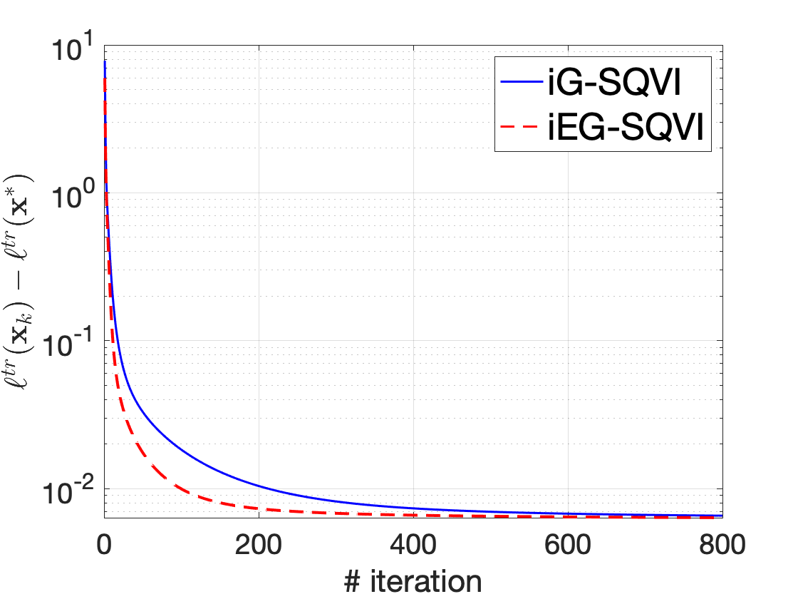
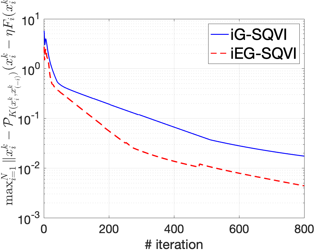
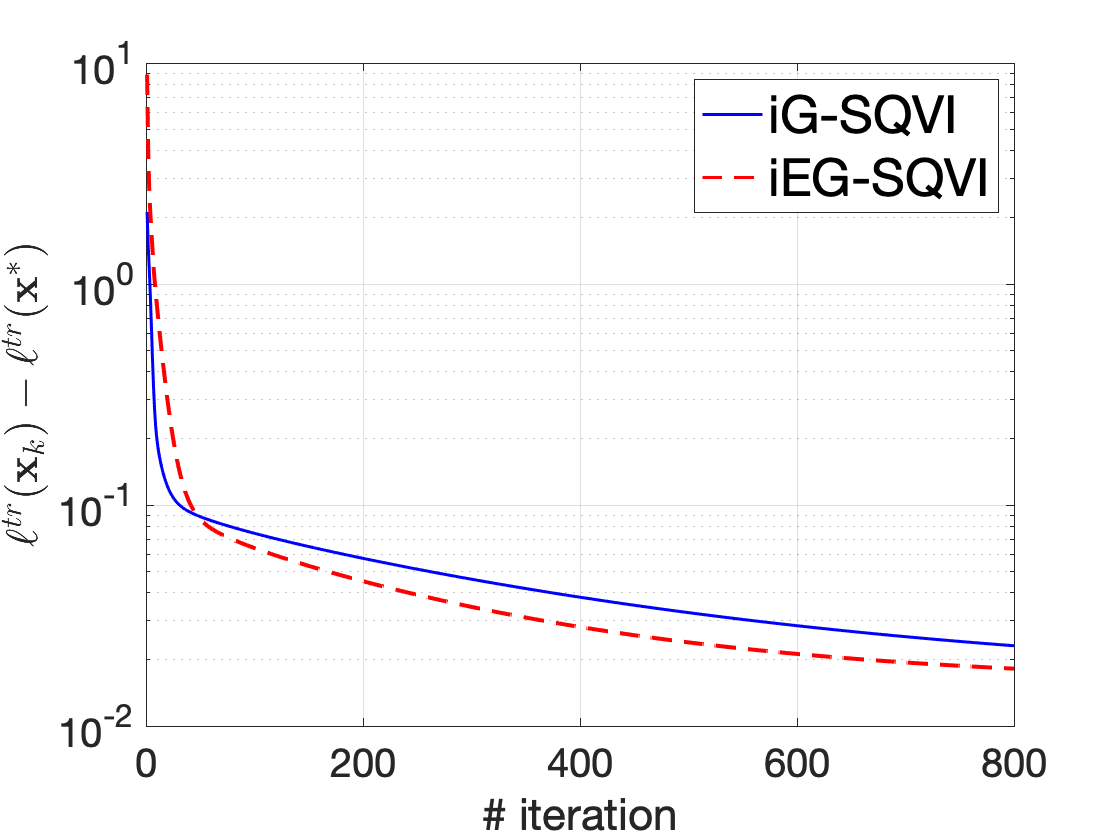
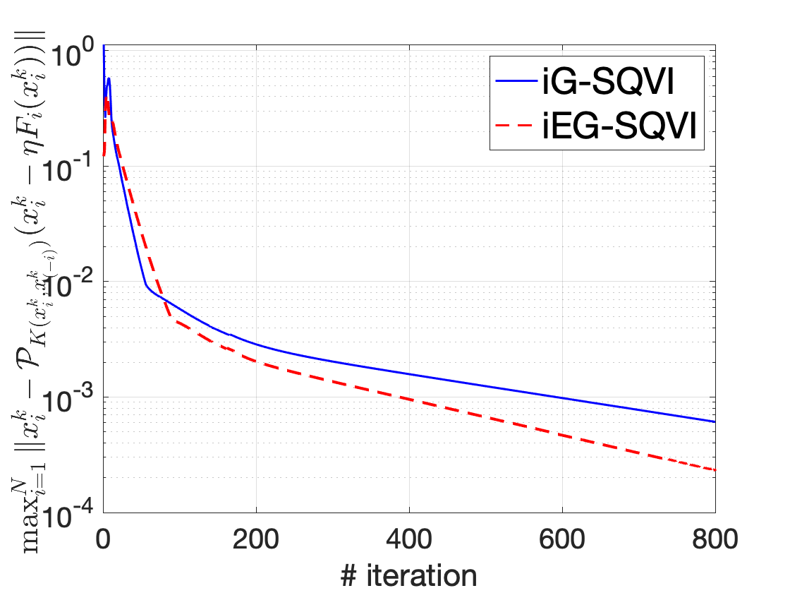
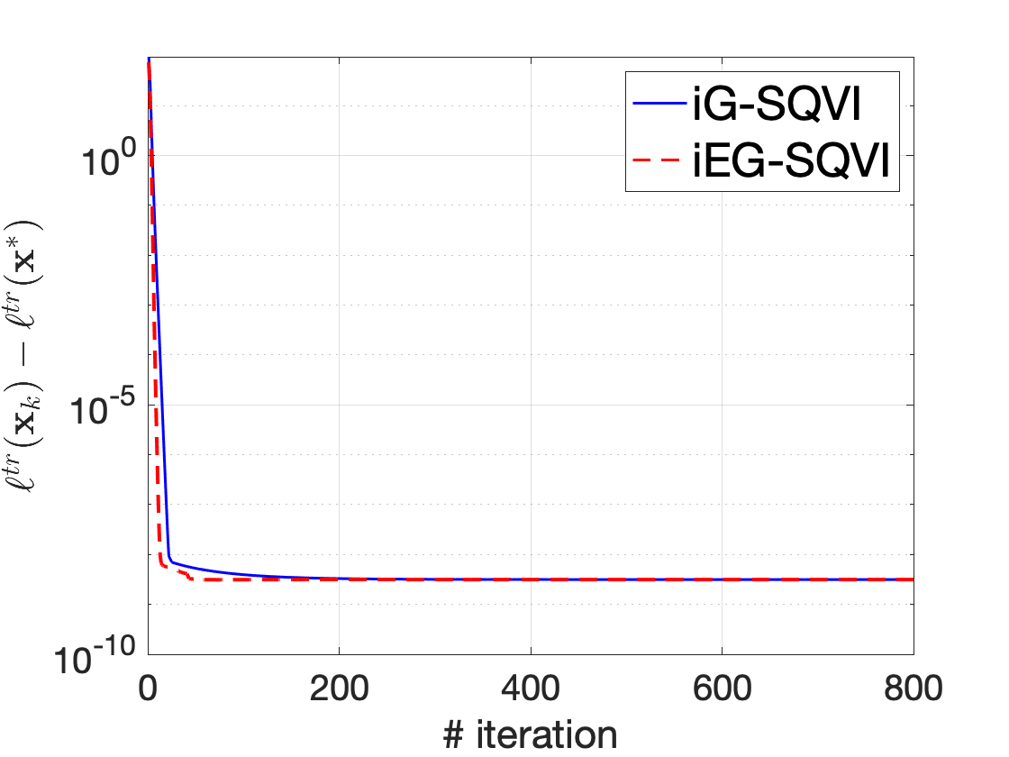
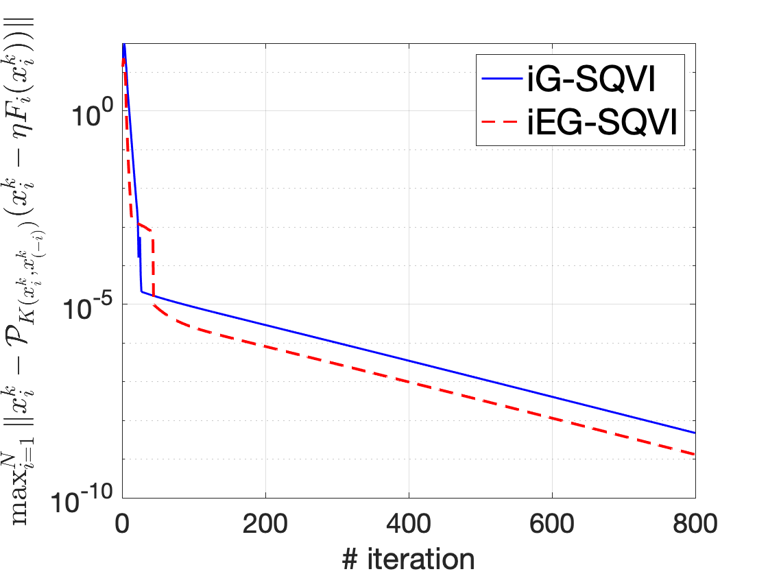
Figure 1: Comparison of iG-SQVI and iEG-SQVI: (Top) for the triazines dataset with 180 data points and 60 features, (Middle) for the eunite2001 dataset with 320 data points and 16 features, (Bottom) for a synthetic dataset with 250 data points and 25 features.

Consider a collection of $N$ players each having a model parameter $x_{i}\in\mathbb{R}^{d}$. Define $\mathbf{x}\triangleq[x_{i}]_{i=1}^{N}$, and suppose there is a shared training dataset $D^{\text{tr}}$ and each player possesses an individual validation dataset $D^{\text{val}}_{i}$. The goal is to find a model parameter $\mathbf{x}$ by minimizing the training loss $\ell^{\text{tr}}(x)$ while each player improves its model parameter based on their validation set by minimizing $\ell^{\text{val}}_{i}(x_{i})$. This problem can be formulated as the following bilevel GNE:

$$\min_{x_{i}\in\mathbb{R}^{d}}\ \ell^{\text{val}}_{i}(x_{i})$$

$$x_{i}\in\mbox{argmin}_{x_{i}\in K_{i}}\ell^{\text{tr}}\left(x_{i},x_{(-i)}^{*}\right).$$

In this experiment, we define $\ell^{\text{val}}_{i}(x_{i})\triangleq\frac{1}{2}\|A_{i}^{\text{val}}x_{i}-b_{i}^{\text{val}}\|^{2},$ where $A_{i}^{\text{val}}\in\mathbb{R}^{n\times d}$ and $b_{i}^{\text{val}}\in\mathbb{R}^{n\times 1}$, and $\ell^{\text{tr}}(x)\triangleq\frac{1}{2}\|A^{\text{tr}}\mathbf{x}-b^{\text{tr}}\|^{2},$ where $A^{\text{tr}}\in\mathbb{R}^{Nn\times Nd}$ and $b^{\text{tr}}\in\mathbb{R}^{Nn\times 1}$ and $X_{i}=\{x_{i}\mid\|x_{i}\|\leq\lambda\}$ for some $\lambda>0$. One can show that this problem can ve formulated as (SQVI) by choosing $K(x)=\Pi_{i=1}^{N}K_{i}(x_{i},x_{(-i)})$, where

$$K_{i}(x_{i},x_{(-i)})=\mbox{argmin}_{x_{i}\in X_{i}}\frac{1}{2}\left\|A_{i}^{\text{tr}}x_{i}+A_{(-i)}^{\text{tr}}x_{(-i)}-b_{i}^{\text{tr}}\right\|^{2},$$

and $F(x)=[F_{i}(x_{i})]_{i=1}^{N}$ where

$$F_{i}(x_{i})=(A_{i}^{\text{val}})^{T}(A_{i}^{\text{val}}x_{i}-b_{i}^{\text{val}}).$$

Note that, operator $F$ is monotone and satisfies quadratic growth property but it may not be strongly monotone. In Figure 1, we present a performance comparison of our proposed methods. For the triazines dataset [6], we set the number of players $N=6$, for the eunite2001 dataset [6] $N=4$, and for the synthetic dataset $N=10$. In all cases, we utilized $80\%$ of the data points for training and allocated the remaining $20\%$ for validation. To solve the projection inexactly, observe that the sub-problem is a simple bilevel optimization problem. This type of problem has been explored in the literature [15, 35]. Here, following [35], we employed the FISTA algorithm [4] to solve the corresponding regularized problem satisfying Assumption 4. For all the experiments, we execute the inner algorithm for $k\log^{2}(k+1)(1-1\text{e-}3)^{k}$ iterations, and the remaining parameters are selected according to the following table after fine-tuning.

Table 1: Parameter settings after fine-tuning for the algorithms across all datasets

	triazines	eunite2001	synthetic
Stepsize $\eta$	5e-2	3e-1	1e-2
$\bar{\alpha}$	1e-1	5e-1	9e-1
$\bar{b}$	1e-1	5e-1	12e-1
Regularizer	1e0	1e-1	1e-2

In Figure 1, on the left, we compared the suboptimality of the lower-level problem, and on the right, we compared the gap function based on the optimality condition (4). It is evident that both methods converge to the optimal solution. Notably, iEG-SQVI demonstrates a slightly better performance due to a smaller convergence rate factor.

7 Conclusion

This paper focuses on solving a class of monotone stochastic quasi-variational inequality problems where the operator satisfies quadratic growth property. We introduce extra-gradient and gradient-based schemes and characterize the convergence rate and oracle complexity of the proposed methods. To the best of our knowledge, our proposed algorithms are the first with a convergence rate guarantee when dealing with non-strongly monotone SQVI problems, especially when projecting onto the constraints is challenging. In our numerical experiments, we showcase the effectiveness and robustness of our methods in solving over-parameterized regression games. These results mark an important first step in exploring broader scenarios, including monotone and weakly-monotone SQVIs. Future directions also involve delving into distributed and risk-based SQVI problems.

Appendix A Extra Gradient Method

Proof of Corollary 2. (i) By taking expectation from both sides of 5, choosing $N_{k}=N$, and using Assumption 2, the following holds.

$$\mathbb{E}\left[\|x_{T}-{\color[rgb]{0,0,0}\bar{x}_{T}}\|\right] \leq(1-q)^{T}\|x_{0}-{\color[rgb]{0,0,0}\bar{x}_{0}}\|{\color[rgb]{0,0,0}+\bar{\alpha}\beta\bar{b}(1-q)^{T-1}\sum_{k=0}^{T-1}\left(\frac{\eta\nu^{\prime}}{(1-q)^{k}\sqrt{N}}+\mathbb{E}[\|e^{\prime}_{k}\|](1-q)^{-k}\right)}$$

$$\quad{\color[rgb]{0,0,0}+\bar{\alpha}(1-q)^{T-1}\sum_{k=0}^{T-1}\left(\frac{\eta\nu}{(1-q)^{k}\sqrt{N}}+\mathbb{E}[\|e_{k}\|](1-q)^{-k}\right).}$$

Following the similar steps as in the proof of Corollary 1, and defining $D\triangleq\sum_{{\color[rgb]{0,0,0}k=0}}^{{\color[rgb]{0,0,0}\infty}}\tfrac{1}{(k+1)\log^{2}(k+2)}{\color[rgb]{0,0,0}\leq 3.39}$, the following can be obtained.

$$\mathbb{E}\left[\|x_{T}-{\color[rgb]{0,0,0}\bar{x}_{T}}\|\right]\leq{\color[rgb]{0,0,0}(1-q)}^{T}\|x_{0}-{\color[rgb]{0,0,0}\bar{x}_{0}}\|+\frac{\bar{\alpha}\beta\bar{b}\eta\nu^{\prime}}{q\sqrt{N}}+\frac{\bar{\alpha}\eta\nu}{q\sqrt{N}}+{\bar{\alpha}\beta\bar{b}C^{\prime}D(1-q)^{T-1}}+{\bar{\alpha}CD(1-q)^{T-1}}.$$

Now by rearranging the terms, we obtain the desired result:

$$\mathbb{E}\left[\|x_{T}-{\color[rgb]{0,0,0}\bar{x}_{T}}\|\right]\leq{\color[rgb]{0,0,0}(1-q)}^{T}\|x_{0}-{\color[rgb]{0,0,0}\bar{x}_{0}}\|+(1-q)^{T-1}\bar{\alpha}D{(\beta\bar{b}C^{\prime}+C)}+\frac{\bar{\alpha}\eta}{q\sqrt{N}}(\beta\bar{b}\nu^{\prime}+\nu).$$ (A1)

(ii) Let $T=\log_{1/(1-q)}(2\bar{D}/\epsilon)$, $N=\tfrac{4\bar{C}^{2}}{q^{2}\epsilon^{2}}$, and define $\bar{D}\triangleq\|x_{0}-{\color[rgb]{0,0,0}\bar{x}_{0}}\|+\tfrac{\bar{\alpha}D{(\beta\bar{b}C^{\prime}+C)}}{(1-q)}$ and $\bar{C}\triangleq\bar{\alpha}\eta(\beta\bar{b}\nu^{\prime}+\nu)$, then from A1 we have that:

$$\mathbb{E}\left[\|x_{T}-{\color[rgb]{0,0,0}\bar{x}_{T}}\|\right] \leq{\color[rgb]{0,0,0}(1-q)}^{T}\big{(}\|x_{0}-{\color[rgb]{0,0,0}\bar{x}_{0}}\|+(1-q)\bar{\alpha}D{(\beta\bar{b}C^{\prime}+C)\big{)}}+\frac{\bar{\alpha}\eta}{q\sqrt{N}}(\beta\bar{b}\nu^{\prime}+\nu)$$

$$\leq{\color[rgb]{0,0,0}(1-q)}^{T}\bar{D}+\frac{\bar{C}}{q\sqrt{N}}\leq\epsilon,$$

where in the last inequality we used the definition of $T$ and $N$.$\square$

Proof of Corollary 3. (i) When a problem is deterministic, we have that $w=w^{\prime}=0$. Therefore, from inequality 5 one can obtain:

$$\|x_{T}-\bar{x}_{T}\|\leq(1-q)^{T}\|x_{0}-\bar{x}_{0}\|+{\bar{\alpha}\sum_{k=0}^{T-1}(1-q)^{T-k-1}\|e_{k}\|}+{\bar{\alpha}\beta\bar{b}\sum_{k=0}^{T-1}(1-q)^{T-k-1}\|e^{\prime}_{k}\|},$$

where $q\triangleq\bar{\alpha}(1-\beta)(1+\beta\bar{b})\in(0,1)$. Now, taking expectations from both sides of the previous inequality, the following holds:

$$\mathbb{E}\left[\|x_{T}-{\color[rgb]{0,0,0}\bar{x}_{T}}\|\right] \leq{\color[rgb]{0,0,0}(1-q)}^{T}\|x_{0}-{\color[rgb]{0,0,0}\bar{x}_{0}}\|+{\bar{\alpha}\beta\bar{b}(1-q)^{T-1}\sum_{k=0}^{{\color[rgb]{0,0,0}T-1}}\left({\color[rgb]{0,0,0}\mathbb{E}[\|e^{\prime}_{k}\|]}{\color[rgb]{0,0,0}(1-q)}^{-k}\right)}$$

$$\quad+{\bar{\alpha}(1-q)^{T-1}\sum_{k=0}^{{\color[rgb]{0,0,0}T-1}}\left({\color[rgb]{0,0,0}\mathbb{E}[\|e_{k}\|]}{\color[rgb]{0,0,0}(1-q)}^{-k}\right).}$$

Following the similar steps as in the proof of Corollary 1, the following can be obtained:

$$\mathbb{E}\left[\|x_{T}-{\color[rgb]{0,0,0}\bar{x}_{T}}\|\right]\leq{\color[rgb]{0,0,0}\rho}^{T}\|x_{0}-{\color[rgb]{0,0,0}\bar{x}_{0}}\|+\rho^{T-1}\bar{\alpha}D(\beta\bar{b}C^{\prime}+C).$$

(ii) Similar steps as in the proof of Corollary 1 (ii). $\square$

Appendix B Gradient Method

In this section, we prove the convergence results of iG-SQVI algorithm. In our analysis, $e_{k}$ denotes the error of computing the projection operator, i.e., for any $k\geq 0$, $e_{k}\triangleq d_{k}-\mathcal{P}_{K(x_{k})}\left(x_{k}-\eta\frac{\sum_{j=1}^{N_{k}}G(x_{k},\xi_{j,k})}{N_{k}}\right)$ and we define $\bar{w}_{k,N_{k}}\triangleq\tfrac{1}{N_{k}}{\sum_{j=1}^{N_{k}}(G(x_{k},\xi_{j,k})-F(x_{k}))}$.

Proof of Theorem 2. For any $k\geq 0$, we define $\bar{x}_{k}\triangleq\mathcal{P}_{X^{*}}(x_{k})$ where $X^{*}$ denotes the set of optimal solutions of problem (SQVI). From Lemma 2 we conclude that $\bar{x}_{k}=\mathcal{P}_{K(\bar{x}_{k})}[\bar{x}_{k}-\eta F(\bar{x}_{k})]$. Using the update rule of $x_{k+1}$, in Algorithm 2 and the fact that $e_{k}$ denotes the error of computing the projection operator, we obtain the following.

$$\|x_{k+1}-\bar{x}_{k}\|$$

$$=\|(1-\alpha_{k})x_{k}+\alpha_{k}\mathcal{P}_{K(x_{k})}\left[x_{k}-\eta(F(x_{k})+\bar{w}_{k,N_{k}})\right]+{\alpha_{k}e_{k}}-(1-\alpha_{k})\bar{x}_{k}-\alpha_{k}\mathcal{P}_{K(\bar{x}_{k})}\left[\bar{x}_{k}-\eta F(\bar{x}_{k})\right]\|$$

$$\leq\|(1-\alpha_{k})(x_{k}-\bar{x}_{k})\|+\alpha_{k}\|\mathcal{P}_{K(x_{k})}\left[x_{k}-\eta(F(x_{k})+\bar{w}_{k,N_{k}})\right]-\mathcal{P}_{K(\bar{x}_{k})}\left[x_{k}-\eta(F(x_{k})+\bar{w}_{k,N_{k}})\right]\|$$

$$\quad+\alpha_{k}\|\mathcal{P}_{K(\bar{x}_{k})}\left[x_{k}-\eta(F(x_{k})+\bar{w}_{k,N_{k}})\right]-\mathcal{P}_{K(\bar{x}_{k})}\left[\bar{x}_{k}-\eta F(\bar{x}_{k})\right]\|+{\alpha_{k}\|e_{k}\|}$$

$$\leq\|(1-\alpha_{k})(x_{k}-\bar{x}_{k})\|+\alpha_{k}\gamma\|x_{k}-\bar{x}_{k}\|+\alpha_{k}\underbrace{\|x_{k}-\bar{x}_{k}-\eta(F(x_{k})-F(\bar{x}_{k}))\|}_{\text{term (a)}}+\alpha_{k}\eta\|\bar{w}_{k,N_{k}}\|+{\alpha_{k}\|e_{k}\|.}$$ (A2)

By using Definition 1 and Lipschitz continuity, the following can be obtained,

$$\|x_{k}-\bar{x}_{k}-\eta(F(x_{k})-F(\bar{x}_{k}))\|^{2} =\|x_{k}-\bar{x}_{k}\|^{2}+\eta^{2}\|F(x_{k})-F(\bar{x}_{k})\|^{2}-2\eta\langle x_{k}-\bar{x}_{k},F(x_{k})-F(\bar{x}_{k})\rangle$$

$$\leq(1+L^{2}\eta^{2}-2\eta k_{f})\|x_{k}-\bar{x}_{k}\|^{2}$$

$$\implies\text{term(a)}\leq\sqrt{1+L^{2}\eta^{2}-2\eta k_{f}}\|x_{k}-\bar{x}_{k}\|.$$ (A3)

Now by using (B) in (B), defining $\beta\triangleq\gamma+\sqrt{1+L^{2}\eta^{2}-2\eta\mu}$ and $q_{i}\triangleq(1-\beta)\alpha_{i}$ we get the following:

$$\|x_{k+1}-\bar{x}_{k}\| \leq(1-\alpha_{k})\|x_{k}-\bar{x}_{k}\|+\alpha_{k}\eta\|\bar{w}_{k,N_{k}}\|{\color[rgb]{0,0,0}+\alpha_{k}\|e_{k}\|}+\alpha_{k}\left(\gamma+\sqrt{1+L^{2}\eta^{2}-2\eta\mu}\right)\|x_{k}-\bar{x}_{k}\|$$

$$=(1-(1-\beta)\alpha_{k})\|x_{k}-\bar{x}_{k}\|+\alpha_{k}\eta\|\bar{w}_{k,N_{k}}\|+{\alpha_{k}\|e_{k}\|}$$

$$\leq{\prod_{i=0}^{k}(1-q_{i})\|x_{0}-\bar{x}_{k}\|+\alpha_{k}\left(\eta\|\bar{w}_{k,N_{k}}\|+\|e_{k}\|\right)}$$

$$\qquad+\sum_{i=0}^{k-1}\left(\left(\prod_{j=i}^{k-1}(1-q_{j+1})\right)\alpha_{i}\left(\eta\|\bar{w}_{i,N_{i}}\|+\|e_{i}\|\right)\right).$$

Next, by choosing $\alpha_{k}=\bar{\alpha}$, where $0<\bar{\alpha}<1$, and based on the conditions of the theorem, one can easily verify that $\beta<1$ and $q_{k}=q<1$ for all $k\geq 0$. $\square$

Proof of Corollary 4. Taking expectation from both sides of 10, choosing $N_{k}=\lceil\rho^{-2k}\rceil$, and using Assumption 2, one can obtain:

$$\mathbb{E}\left[\|x_{T}-{\color[rgb]{0,0,0}\bar{x}_{T}}\|\right]\leq(1-q)^{T}\|x_{0}-{\color[rgb]{0,0,0}\bar{x}_{0}}\|{\color[rgb]{0,0,0}+\bar{\alpha}(1-q)^{T-1}\sum_{k=0}^{T-1}\left(\eta\nu(\frac{\rho}{1-q})^{k}+\mathbb{E}[\|e_{k}\|](1-q)^{-k}\right).}$$ (A4)

Using the fact that $\sum_{{\color[rgb]{0,0,0}k}=0}^{T-1}({\color[rgb]{0,0,0}\tfrac{\rho}{1-q}})^{{\color[rgb]{0,0,0}k}}=\tfrac{1-(\tfrac{\rho}{1-q})^{T}}{1-\tfrac{\rho}{1-q}}$, in (A4), we conclude that

$$\mathbb{E}\left[\|x_{T}-{\color[rgb]{0,0,0}\bar{x}_{T}}\|\right]\leq{\color[rgb]{0,0,0}(1-q)}^{T}\|x_{0}-{\color[rgb]{0,0,0}\bar{x}_{0}}\|+\bar{\alpha}\eta\nu\frac{\rho^{T}-(1-q)^{T}}{\rho+q-1}+{\bar{\alpha}(1-q)^{T-1}\sum_{k=0}^{{\color[rgb]{0,0,0}T-1}}\left({\color[rgb]{0,0,0}\mathbb{E}[\|e_{k}\|]}{\color[rgb]{0,0,0}(1-q)}^{-k}\right).}$$

Since $\rho\geq 1-q$ and $q\in(0,1)$, one can easily show that $-\frac{(1-q)^{T}}{\rho+q-1}<0$. Hence, from the previous inequality we conclude that

$$\mathbb{E}\left[\|x_{T}-{\color[rgb]{0,0,0}\bar{x}_{T}}\|\right] \leq{\color[rgb]{0,0,0}(1-q)}^{T}\|x_{0}-{\color[rgb]{0,0,0}\bar{x}_{0}}\|+\frac{\bar{\alpha}\eta\nu\rho^{T}}{\rho+q-1}+{\bar{\alpha}\sum_{k=0}^{{\color[rgb]{0,0,0}T-1}}\left(\mathbb{E}[\|e_{k}\|]{\color[rgb]{0,0,0}(1-q)^{T-1-k}}\right)}$$

$$\leq\rho^{T}\|x_{0}-{\color[rgb]{0,0,0}\bar{x}_{0}}\|+\frac{\bar{\alpha}\eta\nu\rho^{T}}{\rho+q-1}+\bar{\alpha}\sum_{k=0}^{{\color[rgb]{0,0,0}T-1}}\left(\mathbb{E}[\|e_{k}\|]\rho^{T-1-k}\right).$$

According to the assumption 4, Algorithm $\mathcal{M}$ has a convergence rate of $C/t_{k}^{2}$ within $t_{k}$ inner steps. By selecting $t_{k}=\tfrac{({k+1})\log^{2}(k+2)}{\rho^{k}}$, we conclude that $\mathbb{E}[\|{e_{k}}\|]\leq\tfrac{C}{t_{k}}=\tfrac{C\rho^{k}}{(k+1)\log^{2}(k+2)}$. By using the tower property of expectation in the previous inequality, one can obtain:

$$\mathbb{E}\left[\|x_{T}-{\color[rgb]{0,0,0}\bar{x}_{T}}\|\right]\leq\rho^{T}\|x_{0}-\bar{x}_{0}\|+\frac{\bar{\alpha}\eta\nu\rho^{T}}{\rho+q-1}+\bar{\alpha}C{\color[rgb]{0,0,0}\rho^{T-1}}\sum_{k=0}^{{\color[rgb]{0,0,0}T-1}}{\color[rgb]{0,0,0}\tfrac{1}{(k+1)\log^{2}(k+2)}}.$$

Using the Cauchy-Schwarz inequality, and using the fact that $\rho\geq 1-q$ the following can be obtained:

$$\mathbb{E}\left[\|x_{T}-{\color[rgb]{0,0,0}\bar{x}_{T}}\|\right]\leq{\color[rgb]{0,0,0}\rho}^{T}\|x_{0}-{\color[rgb]{0,0,0}\bar{x}_{0}}\|++\frac{\bar{\alpha}\eta\nu\rho^{T}}{\rho+q-1}+{\bar{\alpha}C{\color[rgb]{0,0,0}\rho^{T-1}}\sum_{k=0}^{{\color[rgb]{0,0,0}T-1}}\left({\color[rgb]{0,0,0}\tfrac{1}{(k+1)\log^{2}(k+2)}}\right)}.$$

Now, by using the fact that $D\triangleq\sum_{{\color[rgb]{0,0,0}k=0}}^{{\color[rgb]{0,0,0}\infty}}\tfrac{1}{(k+1)\log^{2}(k+2)}{\color[rgb]{0,0,0}\leq 3.39}$, and rearranging the terms, the desired result can be obtained

$$\mathbb{E}\left[\|x_{T}-{\color[rgb]{0,0,0}\bar{x}_{T}}\|\right]\leq{\color[rgb]{0,0,0}\rho}^{T}\|x_{0}-{\color[rgb]{0,0,0}\bar{x}_{0}}\|+{\color[rgb]{0,0,0}\tfrac{\rho^{T}\bar{\alpha}\eta\nu}{\rho+q-1}+\rho^{T-1}\bar{\alpha}CD.}$$

(ii) Similar steps as in the proof of Corollary 1 (ii). $\square$

References

- [1] Z. Alizadeh, A. Jalilzadeh, and F. Yousefian, Randomized lagrangian stochastic approximation for large-scale constrained stochastic nash games, arXiv preprint arXiv:2304.07688, (2023).
- [2] Z. Alizadeh, B. M. Otero, and A. Jalilzadeh, An inexact variance-reduced method for stochastic quasi-variational inequality problems with an application in healthcare, in 2022 Winter Simulation Conference (WSC), IEEE, 2022, pp. 3099–3109.
- [3] A. S. Antipin, N. Mijajlović, and M. Jaćimović, A second-order iterative method for solving quasi-variational inequalities, Computational Mathematics and Mathematical Physics, 53 (2013), p. 258.
- [4] A. Beck and M. Teboulle, A fast iterative shrinkage-thresholding algorithm for linear inverse problems, SIAM journal on imaging sciences, 2 (2009), pp. 183–202.
- [5] D. Bertsekas, A. Nedić, and A. Ozdaglar, Convex analysis and optimization, ser, vol. 1, Athena Scientific, 2003.
- [6] C.-C. Chang and C.-J. Lin, LIBSVM: A library for support vector machines, ACM Transactions on Intelligent Systems and Technology, 2 (2011), pp. 27:1–27:27. Software available at http://www.csie.ntu.edu.tw/~cjlin/libsvm.
- [7] F. Facchinei and C. Kanzow, Generalized nash equilibrium problems, Annals of Operations Research, 175 (2010), pp. 177–211.
- [8] F. Facchinei, C. Kanzow, and S. Sagratella, Solving quasi-variational inequalities via their kkt conditions, Mathematical Programming, 144 (2014), pp. 369–412.
- [9] F. Facchinei and J.-S. Pang, Finite-dimensional variational inequalities and complementarity problems, Springer Science & Business Media, 2007.
- [10] L. Franceschi, P. Frasconi, S. Salzo, R. Grazzi, and M. Pontil, Bilevel programming for hyperparameter optimization and meta-learning, in International conference on machine learning, PMLR, 2018, pp. 1568–1577.
- [11] G. Gurkan, A. Y. Ozge, and S. M. Robinson, Sample-path solution of stochastic variational inequalities, with applications to option pricing, in Proceedings Winter Simulation Conference, J. M. Charnes, D. J. Morrice, D. T. Brunner, and J. J. Swain, eds., IEEE, 1996, pp. 337–344.
- [12] E. Y. Hamedani and N. S. Aybat, A primal-dual algorithm with line search for general convex-concave saddle point problems, SIAM Journal on Optimization, 31 (2021), pp. 1299–1329.
- [13] N. He, A. Juditsky, and A. Nemirovski, Mirror prox algorithm for multi-term composite minimization and semi-separable problems, Computational Optimization and Applications, 61 (2015), pp. 275–319.
- [14] A. Jalilzadeh and U. V. Shanbhag, A proximal-point algorithm with variable sample-sizes (PPAWSS) for monotone stochastic variational inequality problems, in 2019 Winter Simulation Conference (WSC), N. Mustafee, K.-H. G. Bae, S. Lazarova-Molnar, M. Rabe, C. Szabo, P. Haas, and Y.-J. Son, eds., IEEE, 2019, pp. 3551–3562.
- [15] R. Jiang, N. Abolfazli, A. Mokhtari, and E. Y. Hamedani, A conditional gradient-based method for simple bilevel optimization with convex lower-level problem, in International Conference on Artificial Intelligence and Statistics, PMLR, 2023, pp. 10305–10323.
- [16] G. M. Korpelevich, The extragradient method for finding saddle points and other problems, Matecon, 12 (1976), pp. 747–756.
- [17] S. Krilašević and S. Grammatico, Learning generalized nash equilibria in monotone games: A hybrid adaptive extremum seeking control approach, Automatica, 151 (2023), p. 110931.
- [18] J. Li, B. Gu, and H. Huang, Improved bilevel model: Fast and optimal algorithm with theoretical guarantee, arXiv preprint arXiv:2009.00690, (2020).
- [19] Y. Malitsky, Projected reflected gradient methods for monotone variational inequalities, SIAM Journal on Optimization, 25 (2015), pp. 502–520.
- [20] , Proximal extrapolated gradient methods for variational inequalities, Optimization Methods and Software, 33 (2018), pp. 140–164.
- [21] Y. Malitsky and M. K. Tam, A forward-backward splitting method for monotone inclusions without cocoercivity, SIAM Journal on Optimization, 30 (2020), pp. 1451–1472.
- [22] N. Mijajlović and M. Jacimović, A proximal method for solving quasi-variational inequalities, Computational Mathematics and Mathematical Physics, 55 (2015), p. 1981.
- [23] N. Mijajlović, M. Jaćimović, and M. A. Noor, Gradient-type projection methods for quasi-variational inequalities, Optimization Letters, 13 (2019), pp. 1885–1896.
- [24] I. Necoara, Y. Nesterov, and F. Glineur, Linear convergence of first order methods for non-strongly convex optimization, Mathematical Programming, 175 (2019), pp. 69–107.
- [25] A. Nemirovski, Prox-method with rate of convergence o(1/t) for variational inequalities with lipschitz continuous monotone operators and smooth convex-concave saddle point problems, SIAM Journal on Optimization, 15 (2004), pp. 229–251.
- [26] Y. Nesterov, Dual extrapolation and its applications to solving variational inequalities and related problems, Mathematical Programming, 109 (2007), pp. 319–344.
- [27] Y. Nesterov and L. Scrimali, Solving strongly monotone variational and quasi-variational inequalities, Discrete and Continuous Dynamical Systems, 31 (2011), pp. 1383–1396.
- [28] M. A. Noor, New approximation schemes for general variational inequalities, Journal of Mathematical Analysis and applications, 251 (2000), pp. 217–229.
- [29] , Existence results for quasi variational inequalities, Banach Journal of Mathematical Analysis, 1 (2007), pp. 186–194.
- [30] M. A. Noor and W. Oettli, On general nonlinear complementarity problems and quasi-equilibria, Le Matematiche, 49 (1994), pp. 313–331.
- [31] J.-S. Pang and M. Fukushima, Quasi-variational inequalities, generalized nash equilibria, and multi-leader-follower games, Computational Management Science, 2 (2005), pp. 21–56.
- [32] U. Ravat and U. V. Shanbhag, On the existence of solutions to stochastic quasi-variational inequality and complementarity problems, Mathematical Programming, 165 (2017), pp. 291–330.
- [33] I. P. Ryazantseva, First-order methods for certain quasi-variational inequalities in a hilbert space, Computational Mathematics and Mathematical Physics, 47 (2007), pp. 183–190.
- [34] H. Salahuddin, Projection methods for quasi-variational inequalities, Mathematical and Computational Applications, 9 (2004), pp. 125–131.
- [35] S. Samadi, D. Burbano, and F. Yousefian, Achieving optimal complexity guarantees for a class of bilevel convex optimization problems, arXiv preprint arXiv:2310.12247, (2023).
- [36] I. Tsaknakis, M. Hong, and S. Zhang, Minimax problems with coupled linear constraints: Computational complexity and duality, SIAM Journal on Optimization, 33 (2023), pp. 2675–2702.
- [37] P. Tseng, A modified forward-backward splitting method for maximal monotone mappings, SIAM Journal on Control and Optimization, 38 (2000), pp. 431–446.