Non-Hermitian Dirac theory from Lindbladian dynamics

Abstract

This study investigates the intricate relationship between dissipative processes of open quantum systems and the non-Hermitian quantum field theory of relativistic fermionic systems. By examining the influence of dissipative effects on Dirac fermions via Lindblad formalism, we elucidate the effects of the coupling of relativistic Dirac particles with the environment. Employing rigorous theoretical analysis, we explore the impact of dissipative interactions and find the Lyapunov equation of the relativistic dissipation-driven fermionic system. By use of a thermal ansatz, one finds the solution to the Lyapunov equations in terms of a stationary Wigner distribution. Our results describe a non-hermitian fermionic system and provide valuable insights into dissipative quantum phenomena’ fundamental mechanisms in relativistic fermionic systems, advancing our understanding of their behavior in non-equilibrium scenarios.

I Introduction

The theoretical description of the subatomic realms through quantum field theory (QFT) evolved significantly over the past century since Dirac’s pioneering work in quantizing the electromagnetic field [1]. The success of the Hamiltonian paradigm and its philosophical implications became hegemonic in the theoretical studies on QFT. As a consequence, the development of mathematical tools for describing the thermodynamic properties of quantum systems, based on Matsubara’s seminal contributions [2] utilizing the imaginary time formalism (known as Matsubara formalism), further revolutionized our understanding of quantum and cosmological realms. While many physicists embraced the equilibrium framework implicit in the Hamiltonian and reflected on the Matsubara formalism [3], a parallel line of research emerged during this period, focusing on the study of out-of-equilibrium QFT. Prominent figures in this pursuit include J. Schwinger [5], L.P. Kadanoff [4], and L.V. Keldysh [6], who made significant contributions to the field of non-equilibrium QFT.

Despite the notable achievements of out-of-equilibrium quantum field theory (QFT) in describing quantum phenomena, the dominance of the equilibrium paradigm has often led the physics community to overlook the contributions of non-equilibrium QFT tools. This dismissal is often justified by arguments regarding the complexity of the formalism and the perceived difficulty of extracting meaningful information from it. However, embracing the equilibrium assumption without demonstrating its inherent presence in a system can obscure fundamental aspects of matter’s behavior. Notably, this philosophical standpoint hinders a genuine comprehension of the nature of the kinetic equation governing a specific system. Recognizing the significance of non-equilibrium QFT is vital for understanding physical phenomena comprehensively and uncovering essential features beyond the equilibrium framework.

I. Prigogine, a Nobel Prize winner for discovering the so-called dissipative structures [7], identified a unique phenomenon exclusive to systems that are out of equilibrium and therefore in constant motion. This discovery brought significant advances in the understanding of nature, challenging the existing paradigm in physics by focusing on systems that are not static, which, according to Prigogine, systems in equilibrium are the exception, not the norm. According to him, quantum mechanics based on the Copenhagen interpretation could not explain irreversible phenomena, since, when defined in a Hilbert space, has its real eigenvalues and, therefore, preserves time-reversal symmetry [8].

The mathematical framework that describes a similar quantum phenomenon has been shown independently from the seminal works written years before in parallel by V. Gorini, A. Kossakowski, and G. Sudarshan (GKS) [9], and G. Lindblad [10]. The so-called GKSL master equation or Lindbladian is one of the general forms of Markovian master equations describing open quantum systems. The Schrödinger equation is generalized for open quantum systems, e.g. a system weakly coupled to a Markovian reservoir. One uses the term Markovian to describe systems where memory effects are absent, and local (in time) equations can describe the system. Within this framework, the dynamical behavior of the system is no longer unitary, but instead preserves trace and remains completely positive for all initial conditions.

To avoid imposing equilibrium conditions, this study adopts the out-of-equilibrium formalism based on the real-time approach, in contrast to the imaginary time method employed in Matsubara formalism. Specifically, we utilize the Closed-Time-Path (CTP) formalism, originally developed by Schwinger [12] and Keldysh [13]. For a detailed understanding of the formalism, interested readers can refer to references such as Berges et al. [14] and Kamenev [15, 16, 17]. As a consequence of the Lindblad master equation, the emerging Dirac-like Lagrangian has a non-hermitian character. The non-hermitian quantum field theory is a recent field of study, and some interesting features arose as the violation of the Noether theorem that related symmetries and charge conservation, and new sources of phase transitions [19, 20, 21].

This work is organized as follows: In Section II one introduces the main aspects of the Lindblad formalism and its application to the Dirac fermionic system with linear jump operators. By use of the path integral formalism, one reaches the action that describes the Dirac fermionic system and through the generating functional, we find the proper Dyson-Schwinger (DS) equations and show the kinetic equation where the Lyapunov equations arose. In Section III we focus on the electromagnetic response of the open fermionic system. In Section VI we present our final comments and perspectives. Throughout this paper, we will be considering the natural units where $\hbar=k_{b}=c=1$.

II The model :

To study the quantum open system one focuses on the reduced density matrix $\rho$ of the system of interest, where one traces over the environment degrees of freedom. The result is the effective non-equilibrium dynamics governed by the following equation:

$$\partial_{t}\rho=\mathcal{L}\rho\leavevmode\nobreak\ \leavevmode\nobreak\ ,$$ (1)

where

$$\mathcal{L}\rho=-i[H,\rho]+\sum_{i}\lambda_{i}\left({L}_{i}^{\dagger}\rho{L}_{i}-\frac{1}{2}\{{L}_{i}^{\dagger}L_{i},\rho\}\right)\leavevmode\nobreak\ \leavevmode\nobreak\ ,$$ (2)

with $H$ a hermitian operator is an effective Hamiltonian operator and the operators $L_{i}^{\dagger},L_{i}$ are the non-hermitian jump operators and model the coupling with the environment in combination with the positive constants $\lambda_{i}$. Equation (1) is called the Lindblad master equation and when the jump operators vanish, one recovers the Von-Neumann master equation the the density matrix. The systems described by equation (1) are commonly called driven open many-body quantum systems and are the most general open quantum systems with local properties.

Assuming that the fermionic system can be described by fermionic creation/annihilation operators $\hat{a}_{{\bf p},s}$, $\hat{b}_{{\bf p},s}$ that obey $\hat{a}_{{\bf p},s}|0\rangle=\hat{b}_{{\bf p},s}|0\rangle=0$. Particle states are obtained acting the creation operators $\hat{a}_{{\bf p},s}^{\dagger}$ and $\hat{b}_{{\bf p},s}^{\dagger}$ operators correspond to the creation operator for particle and anti-particle, respectively. They respect the Grassmman algebra $\{\hat{a}_{{\bf p},s},\hat{a}_{{\bf p^{\prime}},s^{\prime}}^{\dagger}\}=\{\hat{b}_{{\bf p},s},\hat{b}_{{\bf p^{\prime}},s^{\prime}}^{\dagger}\}=\delta_{ss^{\prime}}\delta_{\bf pp^{\prime}}$ and $\{\hat{a}_{{\bf p},s},\hat{a}_{{\bf p^{\prime}},s^{\prime}}\}=\{\hat{b}_{{\bf p},s},\hat{b}_{{\bf p^{\prime}},s^{\prime}}\}=0$. The simplest fermionic CP-even Hamiltonian can be written as $H_{f}=H_{f,0}+H_{f,nl}$:

$$H_{f}=\sum_{\bf p,s}\epsilon_{\bf p}\left(\hat{a}_{{\bf p},s}^{\dagger}\hat{a}_{{\bf p},s}+\hat{b}_{{\bf p},s}^{\dagger}\hat{b}_{{\bf p},s}\right)\leavevmode\nobreak\ \leavevmode\nobreak\ ,$$ (3)

where $\epsilon_{\bf p}=\sqrt{{\bf p}^{2}+m^{2}}$ . This Hamiltonian (3) describes a fermionic harmonic oscillator. To describe the dynamics of the fermionic quantum system in the presence of an environment with a short memory time, one assumes the simplest jump operators as linear operators as follows:

$$L_{1}=\hat{a}_{{\bf p},s}\leavevmode\nobreak\ \leavevmode\nobreak\ ,\leavevmode\nobreak\ \leavevmode\nobreak\ L_{2}=\hat{a}_{{\bf p},s}^{\dagger}\leavevmode\nobreak\ \leavevmode\nobreak\ ,\leavevmode\nobreak\ \leavevmode\nobreak\ L_{3}=\hat{b}_{{\bf p},s}\leavevmode\nobreak\ \leavevmode\nobreak\ ,\leavevmode\nobreak\ \leavevmode\nobreak\ L_{4}=\hat{b}_{{\bf p},s}^{\dagger}\leavevmode\nobreak\ \leavevmode\nobreak\ .$$ (4)

To simplify the notation, we will use $\hat{c}$ to denote the creation/annihilation operators, where $c=a,b$. The Lindblad equation can be expressed as follows:

$$\mathcal{L}\rho=-i[{H}_{f},\rho]+\sum_{\sigma}\left[\lambda_{1,\sigma}\left(\hat{c}_{\sigma}^{\dagger}\rho\hat{c}_{\sigma}-\frac{1}{2}\{\hat{c}_{\sigma}^{\dagger}\hat{c}_{\sigma},\rho\}\right)\right.+$$

$$\hskip 42.67912pt+\left.\lambda_{2,{\bf p}}\left(\hat{c}_{\sigma}\rho\hat{c}_{\sigma}^{\dagger}-\frac{1}{2}\{\hat{c}_{\sigma}\hat{c}_{\sigma}^{\dagger},\rho\}\right)\right]\leavevmode\nobreak\ \leavevmode\nobreak\ .$$ (5)

where $\sigma=\{{\bf p},s,c\}$ and $\lambda_{i,\sigma}\geq 0$ with $i=1,2$ defines the rate of particle gain and loss of the system, respectively. The sum over $c$ means the sum over the particle and antiparticles.

To express the reduced density matrix in the form of a functional integral, one can construct coherent states $|\Psi_{\bf p,s}\rangle,|\Psi^{c}_{\bf p,s}\rangle$ which obey $\hat{a}_{{\bf p},s}|\Psi_{\bf p,s}\rangle=\Psi_{\bf p,s}|\Psi_{\bf p,s}\rangle$ and $\hat{b}_{{\bf p},s}|\Psi^{c}_{\bf p,s}\rangle=\Psi^{c}_{\bf p,s}|\Psi^{c}_{\bf p,s}\rangle$ the coherent particle/anti-particle state, respectively. The elements $\Psi_{\bf p,s}$ and $\Psi^{c}_{\bf p,s}$ are Grassmann variables. By use of the Grassmann algebra one can write:

$$|\Psi_{\sigma}\rangle=e^{-\Psi_{\sigma}\hat{c}_{\sigma}^{\dagger}}|0\rangle\leavevmode\nobreak\ \leavevmode\nobreak\ ,\leavevmode\nobreak\ \leavevmode\nobreak\ \langle\Psi_{\sigma}|=\langle 0|e^{-\tilde{\Psi}_{\sigma}\hat{c}_{\sigma}}$$ (6)

with $\tilde{\Psi}_{\sigma}$ completely unrelated with $\Psi_{\sigma}$ and where $|0\rangle$ is the vacuum state defined via the identities $\hat{c}_{\sigma}|0\rangle=0$, for $c=a,b$. Can be seen that $\langle\Psi_{\sigma}|\Psi_{\sigma^{\prime}}\rangle=\delta_{\bf pp^{\prime}}\delta_{cc^{\prime}}\delta_{ss^{\prime}}e^{\tilde{\Psi}_{\sigma}\Psi_{\sigma^{\prime}}}$, which means the coherent states are not normalized. Therefore, to fix this feature, one needs to introduce the so-called resolution of unity in the coherent states basis, which can be achieved as follows:

$$\hat{1}=\prod_{\sigma}\int D\Psi_{\sigma}e^{-\tilde{\Psi}_{\sigma}\Psi_{\sigma}}|\Psi_{\sigma}\rangle\langle\Psi_{\sigma}|\leavevmode\nobreak\ \leavevmode\nobreak\ .$$ (7)

with $D\Psi=d\tilde{\Psi}_{\sigma}d\Psi_{\sigma}$. Moreover, with these coherent states, one can write any normally ordered operator in terms of the field $\Psi_{\sigma}$. For instance:

$$\langle\Psi_{\sigma^{\prime}}|\hat{c}^{\dagger}_{\sigma^{\prime}}\hat{c}_{\sigma}|\Psi_{\sigma}\rangle=\delta_{\sigma\sigma^{\prime}}\tilde{\Psi}_{\sigma}\Psi_{\sigma}e^{\tilde{\Psi}_{\sigma}\Psi_{\sigma}}\leavevmode\nobreak\ \leavevmode\nobreak\ .$$ (8)

Thus, the trace of some observable $\mathcal{O}$ is given by:

$$Tr[\mathcal{O}]=\prod_{\sigma}\int D\Psi_{\sigma}e^{-\tilde{\Psi}_{\sigma}\Psi_{\sigma}}\langle\Psi_{\sigma}|\mathcal{O}|-\Psi_{\sigma}\rangle\leavevmode\nobreak\ \leavevmode\nobreak\ .$$ (9)

Now, with these properties, one can construct the functional integral version of the reduced density matrix. The solution of equation (1) and can be formally written as:

$$\rho(t)=\mathbb{T}e^{\int_{t_{0}}^{t}dt\hat{\mathcal{L}}(t)}\rho(t_{0})$$ (10)

where $\mathbb{T}$ represents the time-ordering and $\hat{\mathcal{L}}(t)$ is the general time-dependent Lindbladian super-operator. By use of discretization of time in $N$ slices $\delta_{t}$, labeled as $t_{j}$, $j=0,...,N$, the reduced density matrix at time $t_{j+1}$ can be written as follows:

$$\rho_{j+1}=e^{\delta_{t}\hat{\mathcal{L}}_{j}}\rho_{j}\approx\left(1+\delta_{t}\hat{\mathcal{L}}_{j}\right)\rho_{j}\leavevmode\nobreak\ \leavevmode\nobreak\ .$$ (11)

Due to the structure of the super-operator, one needs to introduce two sets of coherent states basis, $|\Psi_{{\bf p},j}^{+}\rangle$, $|\Psi_{{\bf p},j}^{-}\rangle$, acting from the left and right sides of the Lindbladian super-operator, respectively. Therefore, the reduced density matrix super-operator at $t_{j}$ can be written as:

$$\hat{\rho}_{j} = \prod_{\sigma}\int\mathcal{D}(\Psi_{\sigma,j})e^{-(\tilde{\Psi}^{+}_{\sigma_{j}}\Psi^{+}_{\sigma,j})+(\tilde{\Psi}^{-}_{\sigma_{j}}\Psi^{-}_{\sigma,j})}$$ (12)

$$\hskip 28.45274pt\times|\Psi^{+}_{\sigma,j}\rangle\langle\Psi^{+}_{\sigma,j}|\hat{\rho_{j}}|\Psi^{-}_{\sigma,j}\rangle\langle\Psi^{-}_{\sigma,j}|\leavevmode\nobreak\ \leavevmode\nobreak\ ,$$

with $\mathcal{D}(\Psi_{\sigma,j})=d\Psi^{+}_{\sigma,j}d\Psi^{-}_{\sigma,j}$. The Lindblad super-operator at $t_{j}$ is given by:

$$\hat{\mathcal{L}}_{j}\left[|\Psi^{+}_{\sigma,j}\rangle\langle\Psi^{-}_{\sigma,j}|\right] = -iH_{j}|\Psi^{+}_{\sigma,j}\rangle\langle\Psi^{-}_{\sigma,j}|+$$

$$+i|\Psi^{+}_{\sigma,j}\rangle\langle\Psi^{-}_{\sigma,j}|H_{j}+\sum_{\sigma^{\prime},i}\lambda_{\sigma,i}\left({L}_{\sigma^{\prime},i}^{\dagger}|\Psi^{+}_{\sigma,j}\rangle\langle\Psi^{-}_{\sigma,j}|{L}_{\sigma^{\prime},i}+\right.$$

$$-\frac{1}{2}\left({L}_{\sigma^{\prime},i}^{\dagger}L_{\sigma^{\prime},i}|\Psi^{+}_{\sigma,j}\rangle\langle\Psi^{-}_{\sigma,j}|+|\Psi^{+}_{\sigma,j}\rangle\langle\Psi^{-}_{\sigma,j}|{L}_{\sigma^{\prime},i}^{\dagger}L_{\sigma^{\prime},i}\right)\leavevmode\nobreak\ \leavevmode\nobreak\ .$$

Therefore, the matrix elements of the reduced density matrix in the subsequent instant of time $t_{j+1}$ can be written as:

$$\langle\Psi^{+}_{\sigma,j+1}|\hat{\rho}_{j+1}|\Psi^{-}_{\sigma,j}\rangle=\langle\Psi^{+}_{\sigma,j+1}|\hat{\rho}_{\sigma,j}|\Psi^{-}_{\sigma,j}\rangle+$$

$$\hskip 28.45274pt+\delta_{t}\langle\Psi^{+}_{\sigma,j+1}|\hat{\mathcal{L}}_{j}\left[|\Psi^{+}_{\sigma,j}\rangle\langle\Psi^{-}_{\sigma,j}|\right]|\Psi^{-}_{\sigma,j}\rangle\leavevmode\nobreak\ .$$ (14)

where using the properties of normal and time ordering and also the properties of the coherent states given by $\hat{c}_{\sigma}|\Psi_{\sigma,j}\rangle=\Psi_{\sigma,j}|\Psi_{\sigma,j}\rangle$ and $\langle\Psi_{\sigma,j}|\hat{c}_{\sigma}^{\dagger}=\langle\Psi_{\sigma,j}|\Psi_{\sigma,j}$ one reaches:

$$\langle\Psi^{+}_{\sigma,j+1}|\hat{\mathcal{L}}_{j}\left[|\Psi^{+}_{\sigma,j}\rangle\langle\Psi^{-}_{\sigma,j}|\right]|\Psi^{-}_{\sigma,j}\rangle=$$

$$\langle\Psi^{+}_{\sigma,j+1}|\Psi^{+}_{\sigma,j}\rangle\langle\Psi^{-}_{\sigma,j}|\Psi^{-}_{\sigma,j+1}\rangle$$

$$\times\mathcal{L}\left(\tilde{\Psi}_{\sigma,j+1}^{\pm},\tilde{\Psi}_{\sigma,j}^{\pm},\Psi_{\sigma,j}^{\pm},\Psi_{\sigma,j+1}^{\pm}\right)\leavevmode\nobreak\ \leavevmode\nobreak\ ,$$ (15)

and the function $\mathcal{L}$ depends on the form of the Hamiltonian and the jump operators. Thus, at first order on $\delta_{t}$ one can affirm that:

$$\langle\Psi^{+}_{\sigma,j+1}|\hat{\rho}_{j+1}|\Psi^{-}_{\sigma,j+1}\rangle=$$

$$=\prod_{\sigma}\int\mathcal{D}(\Psi_{\sigma,j})e^{\delta_{t}\mathcal{K}\left(\Psi\right)}\langle\Psi^{+}_{\sigma,j}|\hat{\rho}_{\sigma,j}|\Psi^{-}_{\sigma,j}\rangle\leavevmode\nobreak\ \leavevmode\nobreak\ ,$$ (16)

with

$$\mathcal{K}\left(\Psi\right) = \mathcal{K}\left(\tilde{\Psi}_{\sigma,j+1},\tilde{\Psi}_{\sigma,j},\Psi_{\sigma,j+1},\Psi_{\sigma,j}\right)=$$ (17)

$$=\frac{\left(\tilde{\Psi}^{+}_{\sigma,j+1}-\tilde{\Psi}^{+}_{\sigma,j}\right)}{\delta_{t}}{\Psi}^{+}_{\sigma}+\tilde{\Psi}^{-}_{\sigma}\frac{\left(\Psi^{-}_{\sigma,j+1}-\Psi^{-}_{\sigma,j}\right)}{\delta_{t}}+$$

$$+\mathcal{L}\left(\tilde{\Psi}_{\sigma,j+1}^{\pm},\tilde{\Psi}_{\sigma,j}^{\pm},\Psi_{\sigma,j}^{\pm},\Psi_{\sigma,j+1}^{\pm}\right)\leavevmode\nobreak\ \leavevmode\nobreak\ .$$

Finally, by iterating expression from eq. (II) from the initial time $t_{0}$ to a final $t_{f}$ in the limit $\delta_{t}\rightarrow 0$ one reaches:

$$\rho=\frac{e^{iS_{f}\left(\tilde{\Psi},\Psi\right)}}{Z}\leavevmode\nobreak\ \leavevmode\nobreak\ ,\leavevmode\nobreak\ \leavevmode\nobreak\ Z=\int\mathcal{D}\left(\tilde{\Psi},\Psi\right)e^{iS_{f}(\tilde{\Psi},\Psi)}\leavevmode\nobreak\ \leavevmode\nobreak\ ,$$ (18)

with

$$S_{f}(\tilde{\Psi},\Psi) = \sum_{\sigma}\int_{t_{0}}^{t_{f}}dt\Bigg{[}\tilde{\Psi}_{\sigma}^{+}i\partial_{t}\Psi_{\sigma}^{+}-\tilde{\Psi}_{\sigma}^{-}i\partial_{t}\Psi_{\sigma}^{-}-$$ (19)

$$-H_{f}\left(\tilde{\Psi}_{\sigma}^{+},\Psi_{\sigma}^{+}\right)+H_{f}\left(\tilde{\Psi}_{\sigma}^{-},\Psi_{\sigma}^{-}\right)+$$

$$-i\sum_{\sigma,i}\lambda_{i,\sigma}\left((L_{i,\sigma}^{*})^{-}L_{i,\sigma}^{+}-\frac{1}{2}(L_{i,\sigma}^{*})^{+}L_{i,\sigma}^{+}+\right.$$

$$\left.-\frac{1}{2}(L_{i,\sigma}^{*})^{-}L_{i,\sigma}^{-}\right)\Bigg{]}\leavevmode\nobreak\ \leavevmode\nobreak\ ,$$

where $\Psi^{\pm}_{\sigma}=\Psi^{\pm}_{\sigma}(t)$, $\tilde{\Psi}^{\pm}_{\sigma}=\tilde{\Psi}^{\pm}_{\sigma}(t)$ and $L_{i,\sigma}^{\pm}=L_{i}\left(\tilde{\Psi}_{\sigma}^{\pm},\Psi_{\sigma}^{\pm}\right)$. Using the Hamiltonian and jump operators defined in eq. (3) and eq. (4), one reaches:

$$S_{f}(\Psi^{\pm})=$$

$$=\sum_{\sigma}\int_{t_{0}}^{t_{f}}dt\Bigg{[}\tilde{\Psi}_{\sigma}^{+}(i\partial_{t}-\epsilon_{\sigma})\Psi_{\sigma}^{+}-\tilde{\Psi}_{\sigma}^{-}(i\partial_{t}-\epsilon_{\sigma})\Psi_{\sigma}^{-}+$$

$$\hskip 28.45274pt-i\lambda_{1,\sigma}\left(\tilde{\Psi}^{-}_{\sigma}\Psi^{+}_{\sigma}-\frac{1}{2}\tilde{\Psi}^{+}_{\sigma}\Psi^{+}_{\sigma}-\frac{1}{2}\tilde{\Psi}^{-}_{\sigma}\Psi^{-}_{\sigma}\right)+$$

$$\hskip 28.45274pt+i\lambda_{2,\sigma}\left(\tilde{\Psi}^{+}_{\sigma}\Psi^{-}_{\sigma}-\frac{1}{2}\tilde{\Psi}^{+}_{\sigma}\Psi^{+}_{\sigma}-\frac{1}{2}\tilde{\Psi}^{-}_{\sigma}\Psi^{-}_{\sigma}\right)\Bigg{]}\leavevmode\nobreak\ \leavevmode\nobreak\ .$$

Note the plus sign in front of $\lambda_{2,\sigma}$ which comes from the anti-Grassmann properties. Furthermore, one can introduce a new basis, the so-called Keldysh basis, given by:

$$\Psi^{1/2}_{\sigma}=\frac{1}{\sqrt{2}}\left(\Psi^{+}_{\sigma}\pm\Psi^{-}_{\sigma}\right)\leavevmode\nobreak\ \leavevmode\nobreak\ ,\leavevmode\nobreak\ \leavevmode\nobreak\ \tilde{\Psi}^{1/2}_{\sigma}=\frac{1}{\sqrt{2}}\left(\tilde{\Psi}^{+}_{\sigma}\mp\tilde{\Psi}^{-}_{\sigma}\right)\leavevmode\nobreak\ \leavevmode\nobreak\ .$$ (20)

So, the action can be rewritten as:

$$S_{f}=\sum_{\sigma}\int_{t_{0}}^{t_{f}}dt$$

$$\begin{pmatrix}\tilde{\Psi}^{1}_{\sigma}&\tilde{\Psi}^{2}_{\sigma}\end{pmatrix}\begin{pmatrix}i\partial_{t}-\epsilon_{\sigma}-iq_{\sigma}&id_{\sigma}\\ 0&i\partial_{t}-\epsilon_{\sigma}+iq_{\sigma}\end{pmatrix}\begin{pmatrix}\Psi^{1}_{\sigma}\\ \Psi^{2}_{\sigma}\end{pmatrix}\leavevmode\nobreak\ \leavevmode\nobreak\ .$$

where $q_{\sigma}=\frac{1}{2}\left(\lambda_{1,\sigma}+\lambda_{2,\sigma}\right)$ and $d_{\sigma}=\left(\lambda_{1,\sigma}-\lambda_{2,\sigma}\right)$. Finally, based on the assumptions that the dissipative corrections are small, one can write the action in terms of the following four-component Dirac spinors:

$$\psi^{a}({\bf x},t)=\sum_{{\bf p},s}(2\epsilon_{\bf p})^{-1/2}\left(\Psi^{a}_{{\bf p},s}(t)u_{{\bf p},s}e^{i{\bf p}\cdot{\bf x}}+\right.$$

$$\hskip 56.9055pt\left.+(\tilde{\Psi}^{c})^{a}_{{\bf p},s}(t)v_{{\bf p},s}e^{-i{\bf p}\cdot{\bf x}}\right)\leavevmode\nobreak\ \leavevmode\nobreak\ ,$$ (22)

with $a=1,2$ and $u_{{\bf p},s}$, $v_{{\bf p},s}$ are shown in Appendix IV, and defining the Dirac conjugate $\bar{\psi}=\psi^{\dagger}\gamma^{0}$ one has:

$$\bar{\psi}^{a}({\bf x},t)=\sum_{{\bf p},s}(2\epsilon_{\bf p})^{-1/2}\left(\tilde{\Psi}^{a}_{{\bf p},s}(t)\bar{u}_{{\bf p},s}e^{-i{\bf p}\cdot{\bf x}}\right.+$$

$$\hskip 56.9055pt+\left.({\Psi}^{c})^{a}_{{\bf p},s}(t)\bar{v}_{{\bf p},s}e^{i{\bf p}\cdot{\bf x}}\right)\leavevmode\nobreak\ \leavevmode\nobreak\ .$$ (23)

Therefore, the fermionic action takes the final form given by $S_{f}=S_{f,0}+S_{d}$, where:

$$S_{f,0}(\bar{\psi},\psi) =$$ (24)

$$=\int dtd{\bf x}\begin{pmatrix}\bar{\psi}^{1}\leavevmode\nobreak\ \bar{\psi}^{2}\end{pmatrix}\begin{pmatrix}i\not{\partial}-m&0\\ 0&i\not{\partial}-m\end{pmatrix}\begin{pmatrix}\psi^{1}\\ \psi^{2}\end{pmatrix},$$

with $\not{\partial}=\gamma^{\mu}\partial_{\mu}=(\gamma^{0}\partial_{t}-{\bf\gamma}\cdot\nabla)$. The dissipative term reads:

$$S_{d}=\int dtd{\bf x}d{\bf x}^{\prime}\left(\bar{\psi}^{a}(t,{\bf x})\check{\mathcal{D}}_{ab}({\bf x}-{\bf x^{\prime}})\psi^{b}(t,{\bf x^{\prime}})\right)$$

$$\leavevmode\nobreak\ \leavevmode\nobreak\ ,$$ (25)

with

$$\check{\mathcal{D}}_{ab}({\bf x}-{\bf x^{\prime}})=\begin{pmatrix}-i\check{Q}({\bf x}-{\bf x^{\prime}})&i\check{D}({\bf x}-{\bf x^{\prime}})\\ 0&i\check{Q}({\bf x}-{\bf x^{\prime}})\end{pmatrix}\leavevmode\nobreak\ \leavevmode\nobreak\ ,\leavevmode\nobreak\ \leavevmode\nobreak\$$ (26)

where

$$\check{Q}({\bf x}-{\bf x^{\prime}})=\sum_{\bf p}e^{i{\bf p}\cdot({\bf x}-{\bf x^{\prime}})}\check{Q}({\bf p})$$ (27)

and

$$\check{D}({\bf x}-{\bf x^{\prime}})=\sum_{\bf p}e^{i{\bf p}\cdot({\bf x}-{\bf x^{\prime}})}\check{D}({\bf p})\leavevmode\nobreak\ \leavevmode\nobreak\ .$$ (28)

with

$$\check{Q}({\bf p})=\frac{\epsilon_{\bf p}}{2m^{2}}\Big{(}\hat{\not{p}}\left(q_{\bf p}+\tilde{q}_{\bf p}\right)+m\left(q_{\bf p}-\tilde{q}_{\bf p}\right)\Big{)}\leavevmode\nobreak\ \leavevmode\nobreak\ ,$$ (29)

and

$$\check{D}({\bf p})=\frac{\epsilon_{\bf p}}{2m^{2}}\Big{(}\hat{\not{p}}\left(d_{\bf p}+\tilde{d}_{\bf p}\right)+m\left(d_{\bf p}-\tilde{d}_{\bf p}\right)\Big{)}\leavevmode\nobreak\ \leavevmode\nobreak\ ,$$ (30)

where one defines $\hat{p}_{\mu}=(\epsilon_{\bf p},{\bf p})$ is the on-shell four-momentum with $\hat{\not{p}}^{2}=\hat{p}^{2}=m^{2}$ and $\{q,d\},\{\tilde{q},\tilde{d}\}$ the dissipative coefficients for the particles and antiparticles, respectively. The fact that the on-shell momentum appears in equations (27) and (28) is due to the on-shell profile of the particle/antiparticle projectors (defined in Appendix IV). Thus, one shows that the relativistic fermionic system acquires a non-local behavior when interacting with the environment. Particularly, Lindbladian formalism provides a general form to describe the Markovian process of interaction with the external bath via quantum jumps and generates a non-locality in space coordinates even in a free system.

II.1 Dyson-Schwinger equation

Moreover, to construct the Green functions of the system one defines the generating functional as follows:

$$Z[\bar{\eta},\eta]=\int\mathcal{D}[\bar{\psi},\psi]e^{iS[\bar{\psi},\psi,\sigma]+i\int dx\left(\bar{\eta}\psi+\bar{\psi}\eta\right)}\leavevmode\nobreak\ \leavevmode\nobreak\ .$$ (31)

with $\eta^{a},\bar{\eta}^{a}$ the corresponding sources. The generating functional of the connected Green functions $W$ can be written as $W=\frac{1}{i}\ln Z$. Thus, defining the effective action as $\Gamma[\bar{\psi},\psi,\Phi]=W[\bar{\eta},\eta,j]-\int dx[\bar{\eta}\psi+\bar{\psi}\eta+j\sigma]$ one can find the Dyson-Schwinger (DS) equation for the full fermionic propagator $\check{\mathcal{S}}_{ab}(x,y)$ and gives us:

$$\int dy\check{\mathcal{S}}^{-1}_{ab}(x,y)\check{\mathcal{S}}_{bc}(y,z)=\delta_{ac}\delta(x-z),$$ (32)

and, by use of the causality property, the propagator can be rewritten in terms of the retarded, advanced, and Keldysh components as follows:

$$\check{\mathcal{S}}^{-1}_{ab}(x,y)=\begin{pmatrix}(\check{\mathcal{S}}^{R})^{-1}(x,y)&(\check{\mathcal{S}}^{K})^{-1}(x,y)\\ 0&(\check{\mathcal{S}}^{A})^{-1}(x,y)\end{pmatrix}$$ (33)

with

$$(\check{\mathcal{S}}^{R/A})^{-1}(x,x^{\prime})=$$

$$=\left(\left(i\not{\partial}-m\right)\delta({\bf x}-{\bf x}^{\prime})\mp i\check{Q}({\bf x}-{\bf x}^{\prime})\right)\delta(t-t^{\prime})\leavevmode\nobreak\ \leavevmode\nobreak\ .$$

Going further, the fermionic propagator reads:

$$(\check{\mathcal{S}}^{K})^{-1}(x,x^{\prime})=i\check{D}({\bf x}-{\bf x}^{\prime})\delta(t-t^{\prime})\leavevmode\nobreak\ \leavevmode\nobreak\ ,$$

$$\check{\mathcal{S}}_{ab}(x,y)=\begin{pmatrix}\check{\mathcal{S}}^{R}(x,y)&\check{\mathcal{S}}^{K}(x,y)\\ 0&\check{\mathcal{S}}^{A}(x,y)\end{pmatrix}\leavevmode\nobreak\ \leavevmode\nobreak\ ,$$ (36)

such way the DS equation components can be written as follows:

$$\int dy\left(\check{\mathcal{S}}^{R/A}\right)^{-1}(x,y)\check{\mathcal{S}}^{R/A}(y,z)=\delta(x-z),$$ (37)

and

$$\int dy\left(\check{\mathcal{S}}^{R}\right)^{-1}(x,y)\check{\mathcal{S}}^{K}(y,z)=$$ (38)

$$-\int dy\left(\check{\mathcal{S}}^{K}\right)^{-1}(x,y)\check{\mathcal{S}}^{A}(y,z),$$ (39)

The retarded/advanced components of the propagator can be written in momentum space as follows:

$$\check{\mathcal{S}}^{R/A}(x,y)=\sum_{p}e^{ip\cdot(x-y)}\check{\mathcal{S}}^{R/A}(p)$$ (40)

with

$$\check{\mathcal{S}}^{R}(p)=\frac{1}{\not{p}+m-i\check{Q}(\bf p)}\leavevmode\nobreak\ \leavevmode\nobreak\ ,\leavevmode\nobreak\ \leavevmode\nobreak\ \check{\mathcal{S}}^{A}(p)=\frac{1}{\not{p}+m+i\check{Q}({\bf p})}\leavevmode\nobreak\ .$$ (41)

Going further, in general, is a common feature to redefine the anti-Hermitian Keldysh Green function $\mathcal{S}^{K}$ by a Hermitian function $\check{F}=\overline{(\check{F})}$ as $S^{K}=S^{R}\circ\check{F}-\check{F}\circ S^{A}$, where $\check{F}$ is called Wigner distribution and the symbol “$\circ$” represents the convolution operator. By using this parametrization, applying $(\mathcal{S}^{A})^{-1}(z,w)$ from the right side of equation (38) and integrate over $z$, one reaches:

$$\int dy\check{F}(x,y)\left(\check{\mathcal{S}}^{A}\right)^{-1}(y,w)-\int dy(\check{\mathcal{S}}^{R})^{-1}(x,y)\check{F}(y,w)+(\check{\mathcal{S}}^{K})^{-1}(x,w)=0,$$ (42)

and eq.(42) is the kinetic equation in coordinate space. Now, for a given a two-point function $A(x,x^{\prime})$, one can introduce new variables designated by the central point coordinate $X=(x+x^{\prime})/2$ and the relative coordinate $\xi=x-x^{\prime}$, one can perform the Fourier transform on the relative coordinate $\xi$ such that $A(x,x^{\prime})\rightarrow A(X,p)$. This procedure is known as the Wigner transformation. Applying this technique the Eq. (42) one finds that the kinetic equation reads:

$$\frac{i}{2}\{\gamma^{\mu},\frac{\partial\check{F}(X,p)}{\partial X^{\mu}}\}=[\not{p},\check{F}(X,p)]-i\{\check{Q}(p),\ostar\check{F}(X,p)\}+i\check{D}(p)\leavevmode\nobreak\ \leavevmode\nobreak\ .$$ (43)

where

$$A(X,p)\ostar B(X,p)=$$

$$A(X,p)e^{\frac{i}{2}\overleftarrow{\partial}_{X}\overrightarrow{\partial}_{p}-\overleftarrow{\partial}_{p}\overrightarrow{\partial}_{X}}B(X,p)\leavevmode\nobreak\ \leavevmode\nobreak\ .$$ (44)

where the operation with $\ostar$ is known as the Moyal product, and its composition of functions is strongly non-local. Therefore, eq. (43) has infinite derivatives of $\check{F}(X,p)$. Using the Wigner transformation the Keldysh component of the fermionic propagator reads:

$$\check{\mathcal{S}}^{K}(X,p)=\check{\mathcal{S}}^{R}(p)\ostar\check{F}(X,p)-\check{F}(X,p)\ostar\check{\mathcal{S}}^{A}(p)\leavevmode\nobreak\ \leavevmode\nobreak\ .$$ (45)

Moreover, to extract some information, it is useful to assume $\check{F}(X,p)$ independent of $X$ ($\check{F}(X,p)=\check{f}(p)$) and therefore a stationary solution, and apply it to eq. (43) one finds:

$$[\not{p},\check{f}(p)]-i\{\check{Q}(p),\check{f}(p)\}+i\check{D}(p)=0\leavevmode\nobreak\ \leavevmode\nobreak\ .$$ (46)

Eq. (46) is the Lyapunov equation of the relativistic dissipation-driven fermionic system and is one of our main results.

To extract information from eq. (46) is useful to decompose the stationary Wigner distribution $f(p)$ in terms of its spinorial structure as follows:

$$\check{f}(p)=\mathfrak{s}({p})+i\gamma_{5}\mathfrak{p}(p)+\not{\mathfrak{v}}({p})+i\gamma_{5}\not{\mathfrak{a}}({p})+\sigma_{\mu\nu}\mathfrak{t}^{\mu\nu}({p})\leavevmode\nobreak\ \leavevmode\nobreak\ ,$$ (47)

and the non-hermitian terms can be decomposed as follows:

$$\check{Q}(p)=\not{\xi}^{q}(p)+\rho^{q}(p)\leavevmode\nobreak\ \leavevmode\nobreak\ ,\leavevmode\nobreak\ \leavevmode\nobreak\ \check{D}(p)=\not{\xi}^{d}(p)+\rho^{d}(p)\leavevmode\nobreak\ \leavevmode\nobreak\ .$$ (48)

with $\xi^{q}_{\mu}=\frac{\epsilon_{\bf p}}{2m^{2}}\hat{p}_{\mu}(q_{\bf p}+\tilde{q}_{\bf p})$, $\xi^{d}_{\mu}=\frac{\epsilon_{\bf p}}{2m^{2}}\hat{p}_{\mu}(d_{\bf p}+\tilde{d}_{\bf p})$, $\rho^{q}=\frac{\epsilon_{\bf p}}{2m}(q_{\bf p}-\tilde{q}_{\bf p})$ and $\rho^{d}=\frac{\epsilon_{\bf p}}{2m}(d_{\bf p}-\tilde{d}_{\bf p})$. Combining these features on (46) one finds the following set of equations:

$$2\mathfrak{s}\rho^{q}+\rho^{d}+2\mathfrak{v}\cdot\xi^{q}=0\leavevmode\nobreak\ \leavevmode\nobreak\ ,$$ (49a)

$$\mathfrak{a}\cdot p+\mathfrak{p}\rho^{q}=0\leavevmode\nobreak\ \leavevmode\nobreak\ ,$$ (49b)

$$2p^{\mu}\mathfrak{t}_{\beta\mu}+\xi^{d}_{\beta}+2\mathfrak{s}\xi^{q}_{\beta}+2\rho^{q}\mathfrak{v}_{\beta}=0\leavevmode\nobreak\ \leavevmode\nobreak\ ,$$ (49c)

$$-p^{\mu}\leavevmode\nobreak\ {}^{*}\mathfrak{t}_{\beta\mu}-\rho^{q}\mathfrak{a}_{\beta}+\mathfrak{p}p_{\beta}=0\leavevmode\nobreak\ \leavevmode\nobreak\ ,$$ (49d)

$$-\rho^{q}\mathfrak{t}_{\beta\rho}+p_{[\rho}\mathfrak{v}_{\beta]}+\varepsilon_{\beta\rho\mu\nu}\mathfrak{a}^{\mu}(\xi^{q})^{\nu}=0\leavevmode\nobreak\ \leavevmode\nobreak\ .$$ (49e)

with ${}^{*}\mathfrak{t}_{\beta\mu}=\frac{1}{2}\mathfrak{t}^{\nu\rho}\varepsilon_{\beta\mu\nu\rho}$. Although the intricate character of those equations the solution for each component of the Wigner distribution can be found and is given by:

$$\mathfrak{s}(p)=\frac{\rho^{q}\left(b(\xi^{q})^{2}\rho^{q}-\rho^{d}\left(p^{2}+(\rho^{q})^{2}\right)\right)+b(p\cdot\xi^{q})^{2}}{2(\rho^{q})^{2}\left(p^{2}-(\xi^{q})^{2}+(\rho^{q})^{2}\right)-2(p\cdot\xi^{q})^{2}}\leavevmode\nobreak\ \leavevmode\nobreak\ ,$$ (50a)

$$\mathfrak{v}_{\beta}(p)=\frac{(\rho^{d}-b\rho^{q})\left((\rho^{q})^{2}\eta_{\beta\alpha}+p_{\alpha}p_{\beta}\right)(\xi^{q})^{\alpha}}{2(\rho^{q})^{2}\left(p^{2}-(\xi^{q})^{2}+(\rho^{q})^{2}\right)-2(p\cdot\xi^{q})^{2}}\leavevmode\nobreak\ \leavevmode\nobreak\ ,$$

$$\mathfrak{t}_{\rho\beta}=\frac{\rho^{q}(\rho^{d}-b\rho^{q})\left(\xi^{q}_{[\beta}p_{\rho]}\right)}{2(\rho^{q})^{2}\left(p^{2}-(\xi^{q})^{2}+(\rho^{q})^{2}\right)-2(p\cdot\xi^{q})^{2}}$$ (50c)

$$\mathfrak{a}(p)=\mathfrak{p}(p)=0\leavevmode\nobreak\ \leavevmode\nobreak\ ,$$ (50d)

where one defines $b=\frac{d_{\bf p}+\tilde{d}_{\bf p}}{q_{\bf p}+\tilde{q}_{\bf p}}$. Going further, in the next section one restricts the coupling configuration to extract physical insights about the dissipative behavior of the model.

II.2 Thermal Bath:

Assuming the following parametrization of the couplings given by

$$\lambda_{1,{\bf p}}=\kappa\left(1-\tanh\left(\frac{\epsilon_{\bf p}-\mu}{2T}\right)\right)\leavevmode\nobreak\ \leavevmode\nobreak\ ,$$ (51a)

$$\lambda_{2,{\bf p}}=\kappa\left(1+\tanh\left(\frac{\epsilon_{\bf p}-\mu}{2T}\right)\right)\leavevmode\nobreak\ \leavevmode\nobreak\ ,$$ (51b)

$$\tilde{\lambda}_{1,{\bf p}}={\kappa}\left(1-\tanh\left(\frac{\epsilon_{\bf p}+\mu}{2T}\right)\right)\leavevmode\nobreak\ \leavevmode\nobreak\ ,$$ (51c)

and

$$\tilde{\lambda}_{2,{\bf p}}={\kappa}\left(1+\tanh\left(\frac{\epsilon_{\bf p}+\mu}{2T}\right)\right)\leavevmode\nobreak\ \leavevmode\nobreak\ .$$ (51d)

This structure is related to the assumption of the equilibrium of the thermal bath, with fermionic constituents, temperature $T$, and chemical potential $\mu$. Thus, applying this thermal ansatz one finds that the dissipative terms can be written as follows:

$$\xi^{q}_{\mu}=\frac{\epsilon_{\bf p}\kappa}{m^{2}}\hat{p}_{\mu}\leavevmode\nobreak\ \leavevmode\nobreak\ ,\leavevmode\nobreak\ \leavevmode\nobreak\ \rho^{q}=0\leavevmode\nobreak\ \leavevmode\nobreak\ ,$$ (52)

$$\xi^{d}_{\mu}=-\frac{\epsilon_{\bf p}\kappa}{m^{2}}\hat{p}_{\mu}\left(\tanh\left(\frac{\epsilon_{\bf p}-\mu}{2T}\right)+\tanh\left(\frac{\epsilon_{\bf p}+\mu}{2T}\right)\right)\leavevmode\nobreak\ \leavevmode\nobreak\$$ (53)

and

$$\rho^{d}=-\frac{\epsilon_{\bf p}\kappa}{m}\left(\tanh\left(\frac{\epsilon_{\bf p}-\mu}{2T}\right)-\tanh\left(\frac{\epsilon_{\bf p}+\mu}{2T}\right)\right)\leavevmode\nobreak\ \leavevmode\nobreak\ .$$ (54)

Therefore, the stationary solution to the Lyapunov equations can be written as follows:

$$\mathfrak{s}(p)=-\frac{b}{2}\leavevmode\nobreak\ \leavevmode\nobreak\ ,\leavevmode\nobreak\ \leavevmode\nobreak\ \mathfrak{v}_{\mu}(p)=-\frac{\rho^{d}}{2(p\cdot\xi^{q})}p_{\mu}\leavevmode\nobreak\ \leavevmode\nobreak\ .$$ (55)

So, the stationary Wigner distribution is the following:

$$\check{f}(p) = \frac{1}{2}\left(\tanh\left(\frac{\epsilon_{\bf p}-\mu}{2T}\right)+\tanh\left(\frac{\epsilon_{\bf p}+\mu}{2T}\right)\right)+$$

$$+\frac{m\not{p}}{2\left(p\cdot\hat{p}\right)}\left(\tanh\left(\frac{\epsilon_{\bf p}-\mu}{2T}\right)-\tanh\left(\frac{\epsilon_{\bf p}+\mu}{2T}\right)\right)\leavevmode\nobreak\ \leavevmode\nobreak\ .$$

In the case where the thermal bath has a null chemical potential $\mu=0$, i.e., when the particle/antiparticle symmetry is present on the thermal bath, the stationary Wigner distribution simplifies and is the following:

$$\lim_{\mu\rightarrow 0}\check{f}(p)=\tanh\left(\frac{\epsilon_{\bf p}}{2T}\right)=1-2n_{FD}({\bf p})\leavevmode\nobreak\ \leavevmode\nobreak\ ,\leavevmode\nobreak\$$ (57)

with $n_{FD}({\bf p})=\frac{1}{\exp\left(\epsilon_{\bf p}/T\right)+1}$ is the Fermi-Dirac distribution. This result is well-known to respect the fermionic fluctuation-dissipation theorem (FDT) on systems in equilibrium for a fermionic open system given by $\check{\mathcal{S}}^{K}(p)=\check{f}(p)\left(\check{\mathcal{S}}^{R}(p)-\check{\mathcal{S}}^{A}(p)\right)$. Nonetheless, for non-null values of $\mu$ the correspondence disappears due to the spinorial structure of the stationary Wigner distribution. Furthermore, the components of the fermionic propagator are given as:

$$\check{\mathcal{S}}^{R}(p)=\frac{\left(\not{p}+i\not{\xi}^{q}+m\right)}{\left(p+i\xi^{q}\right)^{2}-m^{2}}\leavevmode\nobreak\ \leavevmode\nobreak\ ,\leavevmode\nobreak\ \leavevmode\nobreak\ \check{\mathcal{S}}^{A}(p)=\frac{\left(\not{p}-i\not{\xi}^{q}+m\right)}{\left(p-i\xi^{q}\right)^{2}-m^{2}}$$ (58)

and the poles of the propagator are given by:

$$p_{0}=-i\kappa\left(\frac{\epsilon_{\bf p}}{m}\right)^{2}\pm\sqrt{|{\bf p}|^{2}\left(1+i\frac{\kappa}{m}\left(\frac{\epsilon_{\bf p}}{m}\right)\right)^{2}+m^{2}}$$

$$\hskip 56.9055pt=\mathcal{E}_{\bf p}e^{i\theta_{\bf p}}\leavevmode\nobreak\ \leavevmode\nobreak\ ,$$ (59)

and the energy of the particles is given by the real part, i.e., $Re[p_{0}]=\mathcal{E}_{\bf p}\cos\theta_{\bf p}$ and the decay rate is expressed by the imaginary part $\Gamma_{\bf p}=\mathcal{E}_{\bf p}\sin\theta_{\bf p}$. In fig. 1 one plots the dispersion relation to some representative values of $\kappa$. As it can be seen, the usual dispersion relation for Dirac fermions given by $p_{0}=\sqrt{|{\bf p}|^{2}+m^{2}}$ is represented by the black curve of Fig. 1. As the value of the rate $\kappa/m$ increases one notices that the particle and anti-particle bands start to reform and the gap between the bands becomes smaller. Although the energy spectrum reflects a symmetry between particles/antiparticles, the asymmetry becomes visible when we look at the phase $\theta_{\bf p}$. In fig. 2 one notices that the sign of the quantity $\sin\theta_{\bf p}$ changes from minus to plus at some value of $|{\bf p}|/m$ in which depends on the value of $\kappa$. On the other hand, in fig. 2 the quantity $\sin\theta_{\bf p}$ is positive for any value of $\kappa>0$. Therefore, for the sake of stability one need to have $Im[p_{0}]=\Gamma_{\bf p}<0$, and for $\kappa>0$ one has that the antiparticles are unstable for all ${\bf p}$ but the antiparticles are stable for some values of $|\bf{p}|$ lesser than $\bar{p}(\kappa)$. Now, a useful property can be used to analyze the case $\kappa<0$. The change $\kappa\rightarrow-\kappa$ on eq. II.2 is equivalent to taking its complex conjugate, thus $\kappa\rightarrow-\kappa$ implies that $\theta_{\bf p}\rightarrow-\theta_{\bf p}$. Thus, for $\kappa<0$ one has that the antiparticles are stable for all ${\bf p}$ but the antiparticles are stable for some values of $|\bf{p}|$ greater than $\bar{p}(\kappa)$. The quantity $\bar{p}(\kappa)/m-1$ is shown in fig. 3, and one has two important limits, which are given by $\lim_{\kappa\rightarrow 0}\bar{p}(\kappa)\approx 1.27m$ and $\lim_{\kappa\rightarrow\infty}\bar{p}(\kappa)=m$.

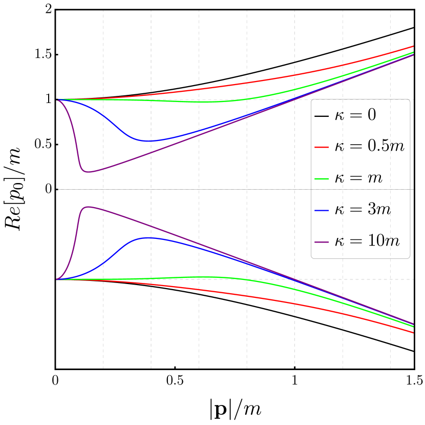
Figure 1: Dispersion relation for the dissipative-driven fermionic particle for some representative values of $\kappa$.

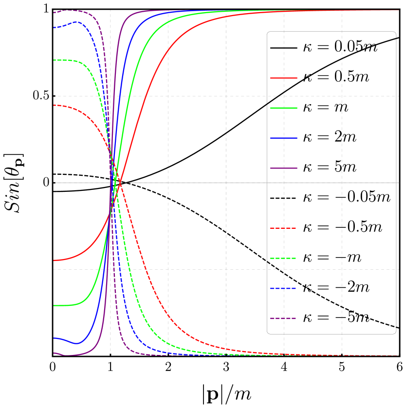
Figure 2: Plot of $\sin\theta_{\bf p}$ as a function of $|{\bf p}|/m$ for $\kappa>0$ and for $\kappa<0$ (both for particles).

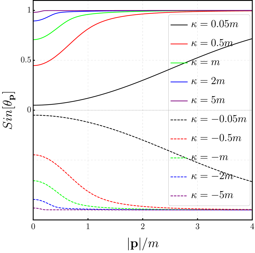
Figure 3: Plot of $\sin\theta_{\bf p}$ as a function of $|{\bf p}|/m$ for $\kappa>0$ and for $\kappa<0$ (both for antiparticles).

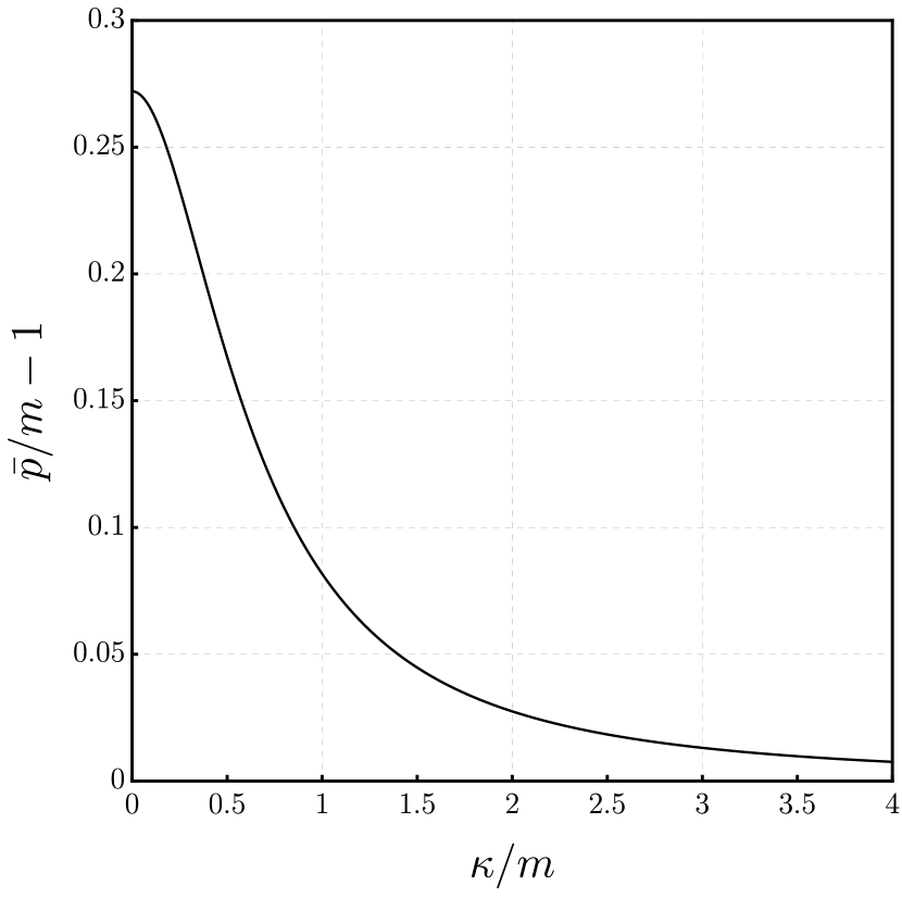
Figure 4: Plot of $\bar{p}/m-1$ as a function of $\kappa/m$.

II.3 Electromagnetic response:

To analyze the behavior of the fermionic system under the presence of an external electromagnetic field we link the fermions to the Electromagnetic field through the covariant derivative operator $D_{\mu}=\partial_{\mu}-ieA_{\mu}$, following the U(1) gauge symmetry principle. Nonetheless, in the out-of-equilibrium paradigm, one must introduce two fields $A_{\mu}^{+},A_{\mu}^{-}$ which interact with the system from the left and right sides. Moreover, rewriting the EM field in terms of classical and quantum fields as follows:

$$A_{\mu}^{cl}=\frac{1}{2}\left(A_{\mu}^{+}+A_{\mu}^{-}\right)\leavevmode\nobreak\ \leavevmode\nobreak\ ,\leavevmode\nobreak\ \leavevmode\nobreak\ A_{\mu}^{q}=\frac{1}{2}\left(A_{\mu}^{+}-A_{\mu}^{-}\right)\leavevmode\nobreak\ \leavevmode\nobreak\ ,$$ (60)

one can write the interaction action:

$$S_{int}=e\int dtd{\bf x}\Bigg{[}\begin{pmatrix}\bar{\psi}^{1}\leavevmode\nobreak\ \bar{\psi}^{2}\end{pmatrix}\begin{pmatrix}\not{A}^{cl}&\not{A}^{q}\\ \not{A}^{q}&\not{A}^{cl}\end{pmatrix}\begin{pmatrix}\psi^{1}\\ \psi^{2}\end{pmatrix}\Bigg{]}$$

$$\hskip 28.45274pt=e\int dtd{\bf x}\bar{\psi}^{a}\gamma^{\mu}\psi^{b}A^{c}_{\mu}(\hat{\sigma}_{c})_{ab}\leavevmode\nobreak\ \leavevmode\nobreak\ ,$$ (61)

where $a,b,c=\{cl,q\}$ and $\hat{\sigma}^{cl}=\begin{pmatrix}1&0\\ 0&1\end{pmatrix}$, $\hat{\sigma}^{q}=\begin{pmatrix}0&1\\ 1&0\end{pmatrix}$. The presence of the quantum source field violates causality but they are non-physical and only serve as auxiliary fields to generate observables. The electronic current can be calculated by application of a functional derivative as follows:

$$j^{c}_{\mu}(x)=\frac{\delta lnZ[A]}{\delta A^{\mu}_{c}(x)}\Bigg{|}_{A=0}=ieTr\Big{[}\gamma_{\mu}\check{\mathcal{S}}^{ab}(x,x)\left(\hat{\sigma^{c}}\right)_{ab}\Big{]}\leavevmode\nobreak\ .$$ (62)

The physical current is coupled to the quantum component of the field and the causality of the action is restored by taking the quantum field as zero. Thus, one finds:

$$j_{\mu}(x)=\frac{\delta lnZ[A]}{\delta A^{\mu}_{q}(x)}\Bigg{|}_{A=0}=ieTr\big{[}\gamma_{\mu}\check{\mathcal{S}}^{K}(x,x)\big{]}\leavevmode\nobreak\ \leavevmode\nobreak\ .$$ (63)

Additionally, looking for stationary configurations one reaches:

$$j^{st}_{\mu} = -4eIm\int dp\leavevmode\nobreak\ \frac{\left(p+i\xi^{q}\right)_{\mu}\mathfrak{s}(p)+m\mathfrak{v}_{\mu}(p)}{(p+i\xi^{q})^{2}-m^{2}}\leavevmode\nobreak\ \leavevmode\nobreak\ .$$

Now, since the component proportional to $\mathfrak{s}$ is an odd function in $p_{0}+i\xi^{q}$, it vanishes. Furthermore, one can split the results into the vacuum and thermodynamic parts, i.e., $j^{st}_{\mu}=j^{st}_{\mu}(T=\mu=0)+j^{st}_{\mu}(T,\mu)$. Can be shown that the vacuum component $j^{st}_{\mu}(T=\mu=0)$ also vanishes. Thus, one can analyze some special limits to extract new information about the result given by eq. (II.3). Is known that the presence of chemical potential generates an effective charge imbalance. For instance, in the limit $T\rightarrow 0$ the quantum electrodynamics result for the charge imbalance is given by $j_{0}/e\approx\frac{\mu^{3}}{6\pi^{2}}$. Going further, one can rewrite the result of eq. (II.3) as follows:

$$j^{st}_{\mu}(T,\mu) = -\frac{e}{(2\pi)^{3}}\int d^{3}{\bf p}\leavevmode\nobreak\ g({\bf p},\kappa,m)\times$$ (65)

$$\left(\tanh\left(\frac{\epsilon_{\bf p}-\mu}{2T}\right)-\tanh\left(\frac{\epsilon_{\bf p}+\mu}{2T}\right)\right)$$

where

$$g({\bf p},\kappa,m)=\frac{1}{2}Im\int_{-\infty}^{\infty}\frac{dp_{0}p_{0}}{(p+i\xi^{q})^{2}-m^{2}}\frac{m^{2}}{p_{0}\epsilon_{\bf p}-{\bf p}^{2}}\leavevmode\nobreak\ \leavevmode\nobreak\ ,$$ (66)

with $g({\bf p},\kappa=0,m)=\pi/2$. The result of eq. (66) is shown in figure 5.

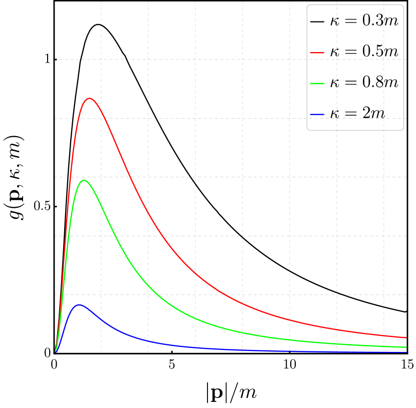
Figure 5: Plot of $g({\bf p},\kappa,m)$ as a function of ${\bf p}/m$ for some values of $\kappa$.

III Final Remarks

In this work, one seeks the formal description of Dirac Lagrangian which arose from the dynamics driven by the Lindblad master equation. The Lindblad equation ensures trace preservation, Hermiticity, and positive semi-definiteness of the reduced density matrix[15]. Interestingly, the Lagrangian that emerges is a non-hermitian model that is an extension of the Dirac Lagrangian. The resulting model is time-local and the dissipative properties that bring non-locality in space coordinates depend on the coupling constants $\lambda_{\sigma}$. By analyzing the retarded propagator one can show that its poles are given by complex quantities and these complex poles are the result of the non-hermitian character of the model.

By use of the Keldysh formalism within the spinor properties, one has successfully determined the Lyapunov equations for stationary Wigner distributions that generalize equilibrium kinetic distributions, using the Dyson-Schwinger equations. Assuming the thermal coupling with the bath that respects the relation $\lambda_{1,{\bf p}}/\lambda_{2,{\bf p}}=\tilde{\lambda}_{1,{\bf p}}/\tilde{\lambda}_{2,{\bf p}}=\exp\left(\epsilon_{\bf p}/T\right)$ we recover the DFT solution of the Wigner distribution of a fermionic stationary system $f(p)=\tanh\left(\frac{\epsilon_{\bf p}}{2T}\right)$, which means that the Fermi-Dirac distribution is a solution of the Lyapunov equations given by eq. 46. However, if the thermal bath has a non-null chemical potential, this asymmetry influences the couplings in such a way the DFT is broken, and a much richer and more complex structure arises from the Lyapunov equations.

Because of the memory-less character typical of Markovian dynamics, the dependence on the initial conditions does not appear in the model presented. Thus, one interesting application of our model can be in the description of the particle/antiparticle asymmetry in the universe, since this asymmetry could be explained by the proper dynamics of the system instead of a problem of some cosmological initial conditions.

Furthermore, if one generalizes the couplings to the bath to include the chirality of the particles one can find the non-hermitian terms $\bar{\psi}\gamma_{5}\psi$ and $\bar{\psi}\gamma_{5}\gamma_{\mu}\psi$ [19, 20, 21]. Another way to describe more general systems is to introduce extra terms to the Hamiltonian, as $(\hat{a}^{2}+h.c.)$ terms. In condensed matter, this kind of term generates the so-called quantum heating effects [25, 26] and can bring interesting modifications to the fermionic system described in this work. The generalization of coupling with the bath to a non-linear version can generate new phenomena as well.

Also, one delves into the intricacies of a fermionic linear system that exhibits unique stationary states confined to the phase space. It is observed that irrespective of the initial state, the system approaches this stationary state exponentially. However, it is important to note that multiple possible scenarios can be observed in linear systems. In some cases, the system can be destabilized, resulting in an exponential runaway behavior. Nonlinearities in the system, as Nambu-Jona-Lasinio models [27, 28], can eventually curtail the instability. This aspect of system behavior governed by nonlinearities will be the focus of future research.

IV Appendix

This appendix shows the orthonormalized Dirac eigenvectors used in the article. Starting from the Dirac equation in four dimensions, one has:

$$(i\gamma^{\mu}\partial_{\mu}-m)\psi(x)=0$$ (67)

with $\psi(x)$ a generic four-component spinor and $\gamma^{\mu}$ the $4\times 4$ Dirac matrices in the Dirac representation can be written as:

$$\gamma^{0}=\begin{pmatrix}1&0\\ 0&-1\end{pmatrix}\leavevmode\nobreak\ \leavevmode\nobreak\ ,\leavevmode\nobreak\ \leavevmode\nobreak\ \gamma^{i}=\begin{pmatrix}0&\sigma^{i}\\ -\sigma^{i}&0\end{pmatrix}\leavevmode\nobreak\ \leavevmode\nobreak\ .$$ (68)

The plane-wave solutions are eigenvectors representing the particle given by:

$$u_{{\bf p},1}=N\begin{pmatrix}1\\ 0\\ \frac{p_{z}}{\epsilon_{\bf p}+m}\\ \frac{p_{+}}{\epsilon_{\bf p}+m}\end{pmatrix}\leavevmode\nobreak\ \leavevmode\nobreak\ ,\leavevmode\nobreak\ \leavevmode\nobreak\ u_{{\bf p},2}=N\begin{pmatrix}0\\ 1\\ \frac{p_{-}}{\epsilon_{\bf p}+m}\\ -\frac{p_{z}}{\epsilon_{\bf p}+m}\end{pmatrix}$$ (69)

The eigenvectors representing the anti-particle are given by:

$$v_{{\bf p},1}=N\begin{pmatrix}\frac{p_{-}}{\epsilon_{\bf p}+m}\\ -\frac{p_{z}}{\epsilon_{\bf p}+m}\\ 0\\ 1\end{pmatrix}\leavevmode\nobreak\ \leavevmode\nobreak\ ,\leavevmode\nobreak\ \leavevmode\nobreak\ v_{{\bf p},2}=N\begin{pmatrix}\frac{p_{z}}{\epsilon_{\bf p}+m}\\ -\frac{p_{+}}{\epsilon_{\bf p}+m}\\ 0\\ 1\\ \end{pmatrix}$$ (70)

with $p_{\pm}=p_{x}\pm ip_{y}$, $N=\sqrt{\epsilon_{\bf p}+m}$ such way $u^{\dagger}u=v^{\dagger}v=2\epsilon_{\bf p}$. The eigenvectors respect the following identities:

$$\bar{u}_{{\bf p},s}u_{{\bf p},s^{\prime}}=2m\delta_{ss^{\prime}}\leavevmode\nobreak\ \leavevmode\nobreak\ ,\leavevmode\nobreak\ \leavevmode\nobreak\ \bar{v}_{{\bf p},s}v_{{\bf p},s^{\prime}}=-2m\delta_{ss^{\prime}}$$ (71)

and

$$\bar{u}_{{\bf p},s}\gamma^{\mu}u_{{\bf p},s^{\prime}}=\bar{v}_{{\bf p},s}\gamma^{\mu}v_{{\bf p},s^{\prime}}=2\hat{p}^{\mu}\delta_{ss^{\prime}}\leavevmode\nobreak\ \leavevmode\nobreak\ ,\leavevmode\nobreak\ \leavevmode\nobreak\ \hat{p}^{\mu}=(\epsilon_{\bf p},{\bf p})\leavevmode\nobreak\ \leavevmode\nobreak\ .$$ (72)

The eigenvectors also obey the completeness relation given by:

$$\sum_{s}u_{{\bf p},s}\bar{u}_{{\bf p},s}=\hat{\not{p}}+m\leavevmode\nobreak\ \leavevmode\nobreak\ ,\leavevmode\nobreak\ \leavevmode\nobreak\ \sum_{s}v_{{\bf p},s}\bar{v}_{{\bf p},s}=\hat{\not{p}}-m\leavevmode\nobreak\ \leavevmode\nobreak\ .$$ (73)

One can write the particle/anti-particle projectors given by:

$$\mathbb{P}=\frac{\hat{\not{p}}+m}{2m}\leavevmode\nobreak\ \leavevmode\nobreak\ ,\mathbb{P}^{c}=\frac{-\hat{\not{p}}+m}{2m}\leavevmode\nobreak\ \leavevmode\nobreak\ ,$$ (74)

such way one can write:

$$\mathbb{P}u_{{\bf p},s}=u_{{\bf p},s}\leavevmode\nobreak\ \leavevmode\nobreak\ ,\leavevmode\nobreak\ \leavevmode\nobreak\ \mathbb{P}^{c}u_{{\bf p},s}=0\leavevmode\nobreak\ \leavevmode\nobreak\ ,\leavevmode\nobreak\ \leavevmode\nobreak\ \mathbb{P}^{c}v_{{\bf p},s}=v_{{\bf p},s}\leavevmode\nobreak\ \leavevmode\nobreak\ ,\leavevmode\nobreak\ \leavevmode\nobreak\ \mathbb{P}v_{{\bf p},s}=0$$ (75)

References

[1] P. A. M. Dirac, The quantum theory of the emission and absorption of radiation. Proceedings of the Royal Society of London. Series A, Containing Papers of a Mathematical and Physical Character, 114(767), 243-265 (1927).
[2] T. Matsubara, A new approach to quantum-statistical mechanics. Progress of theoretical physics, 14(4), 351-378 (1955).
[3] A. A. Abrikosov, L. P. Gor’kov and I. E. Dzyaloshinski. Methods of Quantum Field Theory in Statistical Physics, Dover (1963).
[4] L. P. Kadanoff and G. Baym. Quantum Statistical Mechanics, (New York: Benjamin,
1962).
[5] J. Schwinger, PNAS, 46 (1960), 1401; J. Math. Phys., 2 (1961), 407.
[6] L. V. Keldysh. Zh. Eksp. Teor. Fiz., 47 (1964), 1515; [Sov. Phys. JETP, 20 (1965),
1018].
[7] I. Prigogine, Time, structure and fluctuations. Nobel lecture 8 December. Université Libre de Bruxells, Brussels, Belgium (1977).
[8]T. Petrosky, and I. Prigogine, The Liouville space extension of quantum mechanics. Advances in Chemical Physics, 99, 1-120 (1997).
[9]V. Gorini, A. Kossakowski, and E. C. G. Sudarshan, Completely positive dynamical semigroups of N-level systems, J. Math. Phys. 17, 821 (1976).
[10] G. Lindblad, On the generators of quantum dynamical semigroups, Commun. Math. Phys. 48, 119 (1976).
[11]J. Bardeen, L. N. Cooper, and J.R. Schrieffer, Theory of superconductivity. Physical Review, 108(5), 1175 (1957).
[12] P.C. Martin, and J. Schwinger, Theory of many-particle systems. I. Physical Review, 115(6), 1342 (1959).
[14] J. Berges, Introduction to nonequilibrium quantum field theory, AIP Conf. Proc. 739 (1) (2004) 3–62. arXiv: hep-ph/0409233, doi:10.1063/1.1843591.
[15] A. Kamenev, Field theory of non-equilibrium systems (Cambridge University Press, 2011).
[16] A. Kamenev, and A. Levchenko, Keldysh technique and non-linear -model: basic principles and applications, Adv. Phys, (2010)
[17] F. Thompson and A. Kamenev, Field theory of many-body Lindbladian dynamics. Annals of Physics, 169385, (2023).
[18] Sieberer, L. M., Buchhold, M., and Diehl, S. (2016). Keldysh field theory for driven open quantum systems. Reports on Progress in Physics, 79(9), 096001.
[19]J. Alexandre, C.M. Bender, and P. Millington, Non-Hermitian extension of gauge theories and implications for neutrino physics. Journal of High Energy Physics, 2015 (11), 1-24, (2015).
[20]J. Alexandre, J. Ellis, P. Millington, and D. Seynaeve, Spontaneous symmetry breaking and the Goldstone theorem in non-Hermitian field theories. Physical Review D, 98(4), 045001, (2018)
[21] J. Alexandre, P. Millington, and D. Seynaeve, Symmetries and conservation laws in non-Hermitian field theories. Physical Review D, 96(6), 065027, (2017).
[22] Y.M.P. Gomes, Dyson-Schwinger equation approach to Lorentz symmetry breaking with finite temperature and chemical potential. Physical Review D, 104(1), 015022, (2021).
[23]Y. Hidaka, S. Pu, Q. Wang, and D.L. Yang, Foundations and applications of quantum kinetic theory. Progress in Particle and Nuclear Physics, 103989 (2022).
[24] M. Le Bellac, Thermal field theory. Cambridge university press, 2000.
[25]M. I. Dykman and V. N. Smelyanskiy, Quantum theory of transitions between stable states of a nonlinear oscillator interacting with a medium in a resonant field,
Zh. Eksp. Teor. Fiz., 94, 61 (1988);
[26] M. Marthaler and M. I. Dykman, Switching via quantum activation: A parametrically modulated oscillator, Phys. Rev. A, 73, 042108 (2006).
[27] Y. Nambu, and G. Jona-Lasinio, Dynamical model of elementary particles based on an analogy with superconductivity. I. Physical Review, 122(1), 345 (1961).
[28] Y. Nambu, and G. Jona-Lasinio, Dynamical model of elementary particles based on an analogy with superconductivity. II. Physical Review, 124(1), 246.