Robust Bichromatic Classification using Two Lines

Abstract

Given two sets $R$ and $B$ of at most $n$ points in the plane, we present efficient algorithms to find a two-line linear classifier that best separates the “red” points in $R$ from the “blue” points in $B$ and is robust to outliers. More precisely, we find a region $\mathcal{W}_{B}$ bounded by two lines, so either a halfplane, strip, wedge, or double wedge, containing (most of) the blue points $B$, and few red points. Our running times vary between optimal $O(n\log n)$ and $O(n^{4})$, depending on the type of region $\mathcal{W}_{B}$ and whether we wish to minimize only red outliers, only blue outliers, or both.

1 Introduction

Let $R$ and $B$ be two sets of at most $n$ points in the plane. Our goal is to best separate the “red” points $R$ from the “blue” points $B$ using at most two lines. That is, we wish to find a region $\mathcal{W}_{B}$ bounded by lines $\ell_{1}$ and $\ell_{2}$ containing (most of) the blue points $B$ so that the number of points $k_{R}$ from $R$ in the interior $\operatorname{int}(\mathcal{W}_{B})$ of $\mathcal{W}_{B}$ and/or the number of points $k_{B}$ from $B$ in the interior of the region $\mathcal{W}_{R}=\mathbb{R}^{2}\setminus\mathcal{W}_{B}$ is minimized. We refer to these subsets $\mathcal{E}_{R}=R\cap\operatorname{int}(\mathcal{W}_{B})$ and $\mathcal{E}_{B}=B\cap\operatorname{int}(\mathcal{W}_{R})$ as the red and blue outliers, respectively, and define $\mathcal{E}=\mathcal{E}_{R}\cup\mathcal{E}_{B}$ and $k=k_{R}+k_{B}$.

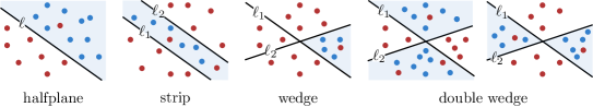
Figure 1: We consider separating $R$ and $B$ by at most two lines. This gives rise to four types of regions $\mathcal{W}_{B}$; halfplanes, strips, wedges, and two types of double wedges; hourglasses and bowties.

It follows that the region $\mathcal{W}_{B}$ is either: $(i)$ a halfplane, $(ii)$ a strip bounded by two parallel lines $\ell_{1}$ and $\ell_{2}$, $(iii)$ a wedge, i.e. one of the four regions induced by a pair of intersecting lines $\ell_{1},\ell_{2}$, or $(iv)$ a double wedge, i.e. two opposing regions induced by a pair of intersecting lines $\ell_{1},\ell_{2}$. See Figure 1. We can reduce the case that $\mathcal{W}_{B}$ would consist of three regions to the wedge case by recoloring the points. We present efficient algorithms to compute an optimal region $\mathcal{W}_{B}$, minimizing either $k_{R}$, $k_{B}$, or $k$, for each of these cases. See Table 1.

Motivation and related work.

Classification is a key problem in computer science. The input is a labeled set of points and the goal is to obtain a procedure that given an unlabeled point assigns it a label that “fits it best”, considering the labeled points. Classification has many direct applications, e.g. identifying SPAM in email messages, or tagging fraudulent transactions [18, 20], but is also the key subroutine in other problems such as clustering [1].

We restrict our attention to binary classification where our input is a set $R$ of red points and a set $B$ of blue points. Popular binary classifiers such as support vector machines (SVMs) [10] attempt to find a hyperplane that “best” separates the red points from the blue points. We can compute if $R$ and $B$ can be perfectly separated by a line (and compute such a line if it exists), in $O(n)$ time using linear programming. This extends to finding a separating hyperplane in case of points in $\mathbb{R}^{d}$, for some constant $d$ [17].

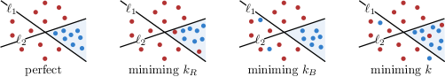
Figure 2: Perfectly separating $R$ and $B$ may require more than one line. When considering outliers, we may allow only red outliers, only blue outliers, or both.

Clearly, it is not always possible to find a hyperplane that perfectly separates the red and the blue points, see for example Figure 2, in which the blue points are actually all contained in a wedge. Hurtato et al. [14, 15] consider separating $R$ and $B$ in $\mathbb{R}^{2}$ using at most two lines $\ell_{1}$ and $\ell_{2}$. In this case, linear programming is unfortunately no longer applicable. Instead, Hurtato et al. present $O(n\log n)$ time algorithms to compute a perfect separator (i.e. a strip, wedge, or double wedge containing all blue points but no red points), if it exists. These results were shown to be optimal [5], and can be extended to the case where $B$ and $R$ contain other geometric objects such as segments or circles, or to include constraints on the slopes [14]. Similarly, Hurtado et al. [16] considered similar strip and wedge separability problems for points in $\mathbb{R}^{3}$. Arkin et al. [4] show how to compute a 2-level binary space partition (a line $\ell$ and two rays starting on $\ell$) separating $R$ and $B$ in $O(n^{2})$ time, and a minimum height $h$-level tree, with $h\leq\log n$, in $n^{O(\log n)}$ time. Even today, computing perfect bichromatic separators with particular geometric properties remains an active research topic [2].

Alternatively, one can consider separation with a (hyper-)plane but allow for outliers. Chan [9] presented algorithms for linear programming in $\mathbb{R}^{2}$ and $\mathbb{R}^{3}$ that allow for up to $k$ violations –and thus solve hyperplane separation with up to $k$ outliers– that run in $O((n+k^{2})\log n)$ and $O(n\log n+k^{11/4}n^{1/4}\operatorname{polylog}n)$ time, respectively. In higher (but constant) dimensions, no non-trivial solutions are known. For arbitrary (non-constant) dimensions the problem is NP-hard [3]. There is also a fair amount of work that aims to find a halfplane that minimizes some other error measure, e.g. the distance to the farthest misclassified point, or the sum of the distances to misclassified points [7, 13].

Separating points using more general non-hyperplane separators and outliers while incorporating guarantees on the number of outliers seems to be less well studied. Seara [19] showed how to compute a strip containing all blue points, while minimizing the number of red points in the strip in $O(n\log n)$ time. Similarly, he presented an $O(n^{2})$ time algorithm for computing a wedge with the same properties. Armaselu and Daescu [6] show how to compute and maintain a smallest circle containing all red points and the minimum number of blue points. In this paper, we take some initial steps toward the fundamental, but challenging problem of computing a robust non-linear separator that provides performance guarantees.

region $\mathcal{W}_{B}$	minimize $k_{R}$		minimize $k_{B}$		minimize $k$
halfplane	$O(n\log n)$	§4	$O(n\log n)$	§4	$O((n+k^{2})\log n)$	[9]
strip	$\Theta(n\log n)$	[19], §5.1	$O(n^{2}\log n)$	§5.2	$O(n^{2}\log n)$	§5.3
wedge	$O(n^{2})$	[19]
	$\Theta(n\log n)$	§6.1	$O(n^{3}\log n)$	§6.2	$O(n^{4})$	§3.1
double wedge	$O(n^{2}\log n)$	§7	$O(n^{2}\log n)$	§7	$O(n^{4})$	§3.1
$\alpha$-double wedge	$O(n^{2}/\alpha)$	§7	$O(n^{2}\log n)$		$O(n^{4})$

Table 1: An overview of our results.

Results.

We present efficient algorithms for computing a region $\mathcal{W}_{B}=\mathcal{W}_{B}(\ell_{1},\ell_{2})$ defined by at most two lines $\ell_{1}$ and $\ell_{2}$ containing only the blue points, that are robust to outliers. Our results depend on the type of region $\mathcal{W}_{B}$ we are looking for, i.e. halfplane, strip, wedge, or double wedge, as well as on the type of outliers we allow: red outliers (counted by $k_{R}$), blue outliers (counted by $k_{B}$), or all outliers (counted by $k$). Refer to Table 1 for an overview.

Our main contributions are efficient algorithms for when $\mathcal{W}_{B}$ is really bounded by two lines. In all but two cases, we improve over the somewhat straightforward $O(n^{4})$ time algorithm of generating a (discrete set) of $O(n^{4})$ candidate regions $\mathcal{W}_{B}(\ell_{1},\ell_{2})$ and explicitly computing how many outliers such a region produces (covered in Section 3). In particular, in the versions of the problem where we wish to minimize the number of red outliers $k_{R}$, we achieve significant speedups. For example, we can compute an optimal wedge $\mathcal{W}_{B}$ containing $B$ and minimizing $k_{R}$ in optimal $\Theta(n\log n)$ time. This improves the earlier $O(n^{2})$ time algorithm from Seara [19].

We use two forms of duality to achieve these results. First, we use the standard duality transform to map points to lines, and lines to points. This allows various structural insights into the problem. For example, in the case of wedges and double wedges we are now searching for particular types of line segments. This then allows us to once more, map each point $p\in R\cup B$ into a forbidden region $E_{p}$ in a low-dimensional parameter space, such that: i) every point $s$ in this parameter space corresponds to a region $\mathcal{W}_{B}(s)$, and ii) this region $\mathcal{W}_{B}(s)$ misclassifies point $p$ if and only if this point $s$ lies in $E_{p}$. Hence, we can reduce our problems to computing a point that is contained in few of these forbidden regions, i.e. that has low ply. We then develop efficient algorithms to this end.

Types of double wedges.

In case of double wedges, this does lead us to make a surprising distinction between “hourglass” type double wedges (that contain a vertical line), and the remaining “bowtie” type double wedges. When we do not allow blue outliers (i.e. when we are minimizing $k_{R}$), we can show that there are only $\Theta(n)$ relevant double (bowtie) wedges w.r.t. $B$. In contrast, there can be $\Theta(n^{2})$ relevant hourglass type double wedges. Hence, dealing with such wedges is harder. Bertschinger et al. [8] observed the same behavior when dealing with intersections of double wedges. In case we have some lower bound on the interior angle $\alpha\pi\leq\pi$ of our double wedge $\mathcal{W}_{B}$, we refer to such double wedges as $\alpha$-double wedges, we can rotate the plane by $i\alpha\pi$, for $i\in 0,..,O(1/\alpha)$, and run our bowtie wedge algorithm each of them. In at least one of these copies the optimum $\mathcal{W}_{B}$ is a bowtie type wedge. This then leads to an $O(n^{2}/\alpha)$ time algorithm for minimizing $k_{R}$.

It is not clear how to find a rotation that turns $\mathcal{W}_{B}$ into a bowtie type double wedge if we do not have any bound on $\alpha$. Instead, we can swap the colors of the point sets, and thus attempt to minimize the number $k_{B}$ of blue outliers, while not allowing any red outliers. The second surprise is that this problem is harder to solve. For double wedges, we present an $O(n^{2}\log n)$ time algorithm, while for single wedges our algorithm takes $O(n^{3}\log n)$ time. For these problems, the duality transform unfortunately does not give us as much information.

Outline.

We give some additional definitions and notation in Section 2. In Section 3 we present a characterization of optimal solutions that lead to our simple $O(n^{4})$ time algorithm for any type of wedges, and in Section 4 we show how to extend Chan’s algorithm [9] to handle one-sided outliers. In Sections 5, 6, and 7 we discuss the case when $W_{B}$ is, respectively, a strip, wedge, or double wedge. In each of these sections we separately go over minimizing the number of red outliers $k_{R}$, the number of blue outliers $k_{B}$, and the total number of outliers $k$. We wrap up with some concluding remarks and future work in Section 8.

2 Preliminaries

In this section we discuss some notation and concepts used throughout the paper. For ease of exposition we assume $B\cup R$ contains at least three points and is in general position, i.e. that all coordinate values are unique, and that no three points are colinear.

Notation.

Let $\ell^{-}$ and $\ell^{+}$ be the two halfplanes bounded by line $\ell$, with $\ell^{-}$ below $\ell$ (or left of $\ell$ if $\ell$ is vertical). Any pair of lines $\ell_{1}$ and $\ell_{2}$, with the slope of $\ell_{1}$ smaller than that of $\ell_{2}$, subdivides the plane into at most four interior-disjoint regions $\mathrm{North}(\ell_{1},\ell_{2})=\ell_{1}^{+}\cap\ell_{2}^{+}$, $\mathrm{East}(\ell_{1},\ell_{2})=\ell_{1}^{+}\cap\ell_{2}^{-}$, $\mathrm{South}(\ell_{1},\ell_{2})=\ell_{1}^{-}\cap\ell_{2}^{-}$ and $\mathrm{West}(\ell_{1},\ell_{2})=\ell_{1}^{-}\cap\ell_{2}^{+}$. When $\ell_{1}$ and $\ell_{2}$ are clear from the context we may simply write $\mathrm{North}$ to mean $\mathrm{North}(\ell_{1},\ell_{2})$ etc. We assign each of these regions to either $B$ or $R$, so that $\mathcal{W}_{B}=\mathcal{W}_{B}(\ell_{1},\ell_{2})$ and $\mathcal{W}_{R}=\mathcal{W}_{R}(\ell_{1},\ell_{2})$ are the union of some elements of $\{\mathrm{North},\mathrm{East},\mathrm{South},\mathrm{West}\}$. In case $\ell_{1}$ and $\ell_{2}$ are parallel, we assume that $\ell_{1}$ lies below $\ell_{2}$, and thus $\mathcal{W}_{B}=\mathrm{East}$.

Duality.

We make frequent use of the standard point-line duality [11], where we map objects in primal space to objects in a dual space. In particular, a primal point $p=(a,b)$ is mapped to a dual line $p^{*}:y=ax-b$ and a primal line $\ell:y=ax+b$ is mapped to a dual point $\ell^{*}=(a,-b)$. Note that dualizing an object twice results in the same object, so $(p^{*})^{*}=p$. If in the primal a point $p$ lies above a line $\ell$, then in the dual the line $p^{*}$ lies below the point $\ell^{*}$.

For a set of points $P$ with duals $P^{*}=\{p^{*}\mid p\in P\}$, we are often interested in the arrangement $\mathcal{A}(P^{*})$, i.e. the vertices, edges, and faces formed by the lines in $P^{*}$. Two unbounded faces of $\mathcal{A}(P^{*})$ are antipodal if their unbounded edges have the same two supporting lines. Consider two antipodal outer faces $P$ and $Q$.

Since every line contributes to four unbounded faces, there are $O(n)$ pairs of antipodal faces. We denote the upper envelope of $P^{*}$, i.e. the polygonal chain following the highest line in $\mathcal{A}(P^{*})$, by $\mathcal{U}(P^{*})$, and the lower envelope by $\mathcal{L}(P*)$.

3 Properties of an optimal separator.

Next, we prove some structural properties about the lines bounding the region $\mathcal{W}_{B}$ containing (most of the) the blue points in $B$. First for strips:

Lemma 3.1.

For the strip classification problem there exists an optimum where one line goes through two points and the other through at least one point.

Proof 3.2.

Clearly, we can shrink an optimal strip $\mathcal{W}_{B}(\ell_{1},\ell_{2})$ so that both $\ell_{1}$ and $\ell_{2}$ contain a (blue) point, say $b_{1}$ and $b_{2}$, respectively. Now rotate $\ell_{1}$ around $b_{1}$ and $\ell_{2}$ around $b_{2}$ in counter-clockwise direction until either $\ell_{1}$ or $\ell_{2}$ contains a second point.

Something similar holds for wedges:

Lemma 3.3.

For any wedge classification problem there exists an optimum where both lines go through a blue and a red point.

Proof 3.4.

We first show that any single wedge can be adjusted such that both its lines go through a blue and a red point, without misclassifying any more points. We then show the same for any double wedge. Since this also holds for a given optimum of a wedge classification problem, we obtain the Lemma.

Claim 1.

Let $\mathcal{W}_{B}(\ell_{1},\ell_{2})$ be a single wedge so that there is at least one correctly classified point of each color. There exists a single wedge $\mathcal{W}_{B}(\ell^{\prime}_{1},\ell^{\prime}_{2})$ such that: (1) both $\ell_{1}^{\prime}$ and $\ell_{2}^{\prime}$ go through a red point and a blue point, (2) and $\mathcal{E}(\ell_{1}^{\prime},\ell_{2}^{\prime})\subseteq\mathcal{E}(\ell_{1},\ell_{2})$.

We show how to find $\ell_{1}^{\prime}$ with a fixed $\ell_{2}$. Line $\ell_{2}^{\prime}$ can be found in the same way afterwards while fixing $\ell_{1}^{\prime}$.

W.l.o.g. assume $\mathcal{W}_{B}$ is the $\mathrm{West}$ wedge. Let $B^{\prime}\subseteq B$ be the correctly classified blue points in that wedge. Start with $\ell_{1}^{\prime}=\ell_{1}$ and shift it downwards it until we hit the convex hull $\mathit{CH}(B^{\prime})$. Note that this does not violate (2): no extra red points are misclassified since we only make the $\mathrm{West}$ wedge smaller, and no extra blue points are misclassified because we stop at the first correctly classified one we hit. Rotate $\ell_{1}^{\prime}$ clockwise around $\mathit{CH}(B^{\prime})$ until we hit a red point, at which point we satisfy (1). If $\ell_{1}^{\prime}$ becomes vertical, the naming of the wedges shifts clockwise (e.g. the $\mathrm{West}$ wedge becomes the $\mathrm{North}$ wedge), so we must change $\mathcal{W}_{B}(\ell_{1}^{\prime},\ell_{2}^{\prime})$ and $\mathcal{W}_{R}(\ell_{1}^{\prime},\ell_{2}^{\prime})$ appropriately. If $\ell_{1}^{\prime}$ becomes parallel to $\ell_{2}$, the $\mathrm{East}$ wedge (temporarily) becomes a strip and the $\mathrm{West}$ wedge disappears. Immediately afterwards the strip becomes the $\mathrm{West}$ wedge, and a new empty $\mathrm{East}$ wedge appears. If $B$ is assigned $\mathrm{West}$ or $\mathrm{East}$ at this time we must change $\mathcal{W}_{B}(\ell_{1}^{\prime},\ell_{2}^{\prime})$ and $\mathcal{W}_{R}(\ell_{1}^{\prime},\ell_{2}^{\prime})$ appropriately.

This procedure does not violate (2) because all of $B^{\prime}$ lies on the same side of $\ell_{1}^{\prime}$ at all times, and we never cross red points. It terminates, i.e. we hit a red point before having rotated around the entire convex hull, because we assumed there to be at least one correctly classified red point which must lie outside the $\mathrm{West}$ wedge and therefor outside of $\mathit{CH}(B^{\prime})$.

Now we show the same for double wedges:

Claim 2.

Let $\mathcal{W}_{B}(\ell_{1},\ell_{2})$ be a double wedge so that there is at least one correctly classified point of each color. There exists a double wedge $\mathcal{W}_{B}(\ell^{\prime}_{1},\ell^{\prime}_{2})$ such that: (1) both $\ell_{1}^{\prime}$ and $\ell_{2}^{\prime}$ go through a red point and a blue point, (2) and $\mathcal{E}(\ell_{1}^{\prime},\ell_{2}^{\prime})\subseteq\mathcal{E}(\ell_{1},\ell_{2})$.

We show how to find $\ell_{1}^{\prime}$ with a fixed $\ell_{2}$. Line $\ell_{2}^{\prime}$ can be found in the same way afterwards while fixing $\ell_{1}^{\prime}$.

W.l.o.g. assume $\mathcal{W}_{B}$ is the bowtie consisting of the $\mathrm{West}$ and $\mathrm{East}$ wedges. Consider the dual arrangement $\mathcal{A}(B^{*},R^{*})$, where we want segment $\overline{{\ell_{1}^{*}}\ell_{2}^{*}}$ to intersect blue lines but not red lines. Let $m$ be the supporting line of segment $\overline{{\ell_{1}^{*}}\ell_{2}^{*}}$. Start with ${\ell_{1}^{*}}^{\prime}=\ell_{1}^{*}$. Note that if ${\ell_{1}^{*}}^{\prime}$ ever lies in a face with red and blue segments on its boundary we are done: set ${\ell_{1}^{*}}^{\prime}$ as one of the red-blue intersections, which satisfies (1) and does not change (2). Otherwise we distinguish two cases:

• ${\ell_{1}^{*}}^{\prime}$ lies in an all red face. We can shrink $\overline{{\ell_{1}^{*}}^{\prime}\ell_{2}^{*}}$ by moving ${\ell_{1}^{*}}^{\prime}$ towards $\ell_{2}^{*}$ along $m$ until we enter a bicolored face, in which case we are done. This will not violate (2), since shrinking the segment can only cause it to intersect fewer red lines. We must enter a bicolored face before the segment collapses since we assumed there to be at least one correctly classified blue point. See Figure 3a.

• ${\ell_{1}^{*}}^{\prime}$ lies in an all blue face. We extend $\overline{{\ell_{1}^{*}}^{\prime}\ell_{2}^{*}}$ by moving ${\ell_{1}^{*}}^{\prime}$ along $m$ until either (i) ${\ell_{1}^{*}}^{\prime}$ enters a bicolored face, in which case we are done, or until (ii) ${\ell_{1}^{*}}^{\prime}$ ends up in an outer face which is unbounded in the direction of $m$. This does not violate (2), since extending the segment will only make it intersect more blue lines. See Figure 3b.

  In case (ii), let $F$ be the outer face ${\ell_{1}^{*}}^{\prime}$ ends up in, and let $p^{*}$ be some point on $m$ in $F$. Let $F^{\prime}$ be the antipodal face of $F$, and let $q^{*}$ be some point on $m$ in $F^{\prime}$. See Figure 3c. Observe that segment $\overline{q^{*}\ell_{2}^{*}}$ intersects exactly those lines that segment $\overline{p^{*}\ell_{2}^{*}}$ does not intersect, and the other way around. In the primal, points in the hourglass wedge of $(p,\ell_{2})$ are in the bowtie wedge of $(q,\ell_{2})$. Therefore segment $\overline{p^{*}\ell_{2}^{*}}$ yields the exact same classification $\overline{q^{*}\ell_{2}^{*}}$, after assigning $B$ to the hourglass wedge instead of the bowtie wedge.

  This means we can set ${\ell_{1}^{*}}^{\prime}=q$, change the color assignment appropriately, and shrink segment $\overline{{\ell_{1}^{*}}^{\prime}\ell_{2}^{*}}$ until ${\ell_{1}^{*}}^{\prime}$ lies in a bicolored face. This does not violate (2), since shrinking the segment only makes it intersect fewer blue lines. We must enter a bicolored face before the segment collapses since we assumed there to be at least one corrrectly classified red point.

The above two claims tell us that, given some optimal (double) wedge for a wedge separation problem, we can adjust the wedge until both lines go through a red and a blue point, proving the Lemma.

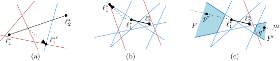
Figure 3: (a)/(b): shrinking/extending segment $\overline{{\ell_{1}^{*}}\ell_{2}^{*}}$ until it reaches a bicolored face. (c): points $p^{*}$ and $q^{*}$ in antipodal outer faces $F$ and $F^{\prime}$. Segment $\overline{p^{*}\ell_{2}^{*}}$ intersects exactly those lines that $\overline{q^{*}\ell_{2}^{*}}$ does not intersect.

3.1 Simple general algorithm

Lemma 3.3 tells us we only have to consider lines through red and blue points. Hence, there is a simple somewhat brute-force algorithm that works for both wedges and double wedges and any type of outliers by considering all pairs of such lines.

Theorem 3.5.

Given two sets of $n$ points $B,R\subset\mathbb{R}^{2}$, we can construct a (double) wedge $\mathcal{W}_{B}$ minimizing either $k_{r}$, $k_{b}$, or $k$ in $O(n^{4})$ time.

Proof 3.6.

By Lemma 3.3 we only have to consider lines through blue and red points. There are $O(n^{2})$ such lines, so $O(n^{4})$ pairs of such lines. We could trivially calculate the number of misclassifications for two fixed lines in $O(n)$ time by iterating through all points, which would result in $O(n^{5})$ total time, but we can improve on this.

Construct the dual arrangement $\mathcal{A}(B^{*}\cup R^{*})$ of $B\cup R$ in $O(n^{2})$ time. A red-blue intersection in the dual $\mathcal{A}(B^{*}\cup R^{*})$ corresponds to a candidate line through a red and a blue point in the primal. Choose two arbitrary red-blue vertices as $\ell_{1}^{*}$ and $\ell_{2}^{*}$, and calculate the number of red and blue points in each of the four wedge regions in $O(n)$ time. Move $\ell_{1}^{*}$ through the arrangement in a depth-first search order, updating the number of points in each wedge at each step. There is only a single point that lies on the other side of $\ell_{1}$ after this movement, so this update can be done in constant time. After every step of $\ell_{1}^{*}$, also move $\ell_{2}^{*}$ through the whole arrangement in depth-first search order, updating the number of points in each wedge, again in constant time. Finally, output the pair of lines that misclassify the fewest points. There are $O(n^{2})$ choices for $\ell_{1}^{*}$, and for each of those there are $O(n^{2})$ choices for $\ell_{2}^{*}$. Since every update takes constant time, this takes $O(n^{4})$ time in total.

4 Single line one-sided outliers

In this section, our goal is to find a single line $\ell$ such that $B\subset\ell^{+}$ and the minimum number $k$ of red points $R\subset\ell^{+}$. Similar to Chan [9] we can solve this using duality and interval counting. The case where we allow a minimum number of blue outliers (but no red outliers) is symmetric.

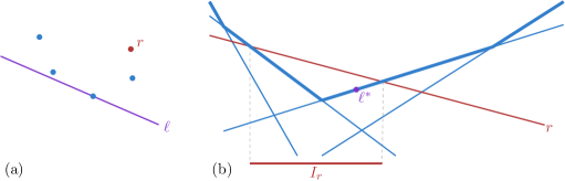
Figure 4: (a) Line $\ell$ misclassifies a red point $r$, in the dual space (b) that means $\ell^{*}\in I_{r}$.

Theorem 4.1.

Given two sets of $n$ points $B,R\subset\mathbb{R}^{2}$, we can find a line with all points of $B$ on one side and as many points of $R$ as possible on the other side in $O(n\log n)$ time.

Proof 4.2.

Dualize the points in $B$ and $R$ to lines. Our goal is then to find a point $\ell^{*}$ that lies above all blue lines, i.e. above the upper envelope $\mathcal{U}(B^{*})$, and above at most $k$ red lines. See Figure 4. Observe that if there exists such a point $\ell^{*}$ we can always shift it downwards until it lies on $\mathcal{U}(B^{*})$ without increasing the number of red lines below $\ell^{*}$ (and while keeping all blue lines below it). Hence, assume without loss of generality that $\ell^{*}$ lies on $\mathcal{U}(B^{*})$.

Since $\mathcal{U}(B^{*})$ is a convex polygonal chain, every red line $r\in R^{*}$ lies on or above $\mathcal{U}(B^{*})$ in a single interval $I_{r}$ along $\mathcal{U}(B^{*})$. Moreover, (the line dual to) $\ell^{*}\in\mathcal{U}(B^{*})$ misclassifies line $r$ if and only if $\ell^{*}\in I_{r}$. Hence, given the set of intervals $\{I_{r}\mid r\in R^{*}\}$ our goal is to find a point $\ell^{*}$ with minimum ply $\Delta(\ell^{*})=|\{I_{r}\mid r\in R^{*}\land\ell^{*}\in I_{r}\}|$, i.e. the number of intervals containing $\ell^{*}$. This can be done in $O(n\log n)$ time by sorting and scanning. Computing $\mathcal{U}(B^{*})$ takes $O(n\log n)$ time, and given a line $r\in R^{*}$, we can compute $I_{r}$ in $O(\log n)$ time by a simple binary search.

5 Separation with a strip

In this section we consider the case where lines $\ell_{1}$ and $\ell_{2}$ are parallel, with $\ell_{2}$ above $\ell_{1}$, and thus $\mathcal{W}_{B}(\ell_{1},\ell_{2})$ forms a strip. We want $B$ to be inside the strip, and $R$ outside. We solve this problem in the dual, where we want to find two points $\ell_{1}^{*}$ and $\ell_{2}^{*}$ with the same $x$-coordinate such that vertical segment $\overline{\ell_{1}^{*}\ell_{2}^{*}}$ intersects the lines in $B^{*}$ but not the lines in $R^{*}$.

5.1 Strip separation with red outliers

We first consider the case where all blue points must be correctly classified, and we minimize the number of red outliers $k_{R}$. We present an $O(n\log n)$ time algorithm to this end. Note that this runtime matches the existing algorithm from Seara [19]. We wish to find a segment $\overline{\ell_{1}^{*}\ell_{2}^{*}}$ that intersects all lines in $B^{*}$, so $\ell_{1}^{*}$ must be above the upper envelope $\mathcal{U}(B^{*})$ and $\ell_{2}^{*}$ must be below the lower envelope $\mathcal{L}(B^{*})$. We can assume $\ell_{1}^{*}$ to lie on $\mathcal{U}(B^{*})$ and $\ell_{2}^{*}$ on $\mathcal{L}(B^{*})$, since shortening $\overline{\ell_{1}^{*}\ell_{2}^{*}}$ can only decrease the number of red lines intersected.

As $\mathcal{U}(B^{*})$ and $\mathcal{L}(B^{*})$ are $x$-monotone, there is only one degree of freedom for choosing our segment: its $x$-coordinate. We parameterize $\mathcal{U}(B^{*})$ and $\mathcal{L}(B^{*})$ over $\mathbb{R}$, our parameter space, such that each point $p\in\mathbb{R}$ corresponds to the vertical segment $\overline{\ell_{1}^{*}\ell_{2}^{*}}$ on the line $x=p$. We wish to find a point in this parameter space whose corresponding segment minimizes the number of red misclassifications, i.e. the number of red intersections. Let the forbidden regions of a red line $r$ be those intervals on the parameter space in which corresponding segments intersect $r$. We distinguish between four types of red lines, as in Figure 5:

• Line $a$ intersects $\mathcal{U}(B^{*})$ in points $a_{1}$ and $a_{2}$, with $a_{1}\leq a_{2}$. Segments with $\ell^{*}_{1}$ left of $a_{1}$ or right of $a_{2}$ misclassify $a$, so $a$ produces two forbidden intervals: $(-\infty,a_{1})$ and $(a_{2},\infty)$.

• Line $b$ intersects $\mathcal{L}(B^{*})$ in points $b_{1}$ and $b_{2}$, with $b_{1}\leq b_{2}$. Similar to line $a$ this produces forbidden intervals $(-\infty,b_{1})$ and $(b_{2},\infty)$.

• Line $c$ intersects $\mathcal{L}(B^{*})$ in $c_{1}$ and $\mathcal{U}(B^{*})$ in $c_{2}$. Only segments between $c_{1}$ and $c_{2}$ misclassify $c$. This gives one forbidden interval: $(\min\{c_{1},c2\},\max\{c_{1},c_{2}\})$.

• Line $d$ intersects neither $\mathcal{U}(B^{*})$ nor $\mathcal{L}(B^{*})$. All segments misclassify $d$. This gives one trivial forbidden region, namely the entire space $\mathbb{R}$.

The above list is exhaustive. Clearly a line can not intersect $\mathcal{U}(B^{*})$ or $\mathcal{L}(B^{*})$ more than twice. Let $b_{1},b_{2}$ be the two blue lines supporting the unbounded edges of $\mathcal{U}(B^{*})$, and note that these are the same two lines supporting the unbounded edges of $\mathcal{L}(B^{*})$. Therefore if a line intersects $\mathcal{U}(B^{*})$ twice it can not intersect $\mathcal{L}(B^{*})$ and vice versa. Additionally, any line intersecting $\mathcal{U}(B^{*})$ once must have a slope between those of $b_{1}$ and $b_{2}$, hence it must also intersect $\mathcal{L}(B^{*})$ once, and vice versa.

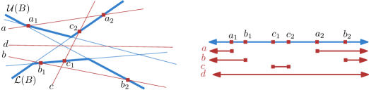
Figure 5: Four types of red lines for strip separation, with restrictions on their parameter space.

Recall that our goal is to find a point with minimum ply in these forbidden regions. We can compute such a point in $O(n\log n)$ time by sorting and scanning. Computing $\mathcal{U}(B^{*})$ and $\mathcal{L}(B^{*})$ takes $O(n\log n)$ time. Given a red line $r\in R^{*}$ we can compute its intersection points with $\mathcal{U}(B^{*})$ and $\mathcal{L}(B^{*})$ in $O(\log n)$ time using binary search (using that $\mathcal{U}(B^{*})$ and $\mathcal{L}(B^{*})$ are convex). Computing the forbidden regions thus takes $O(n\log n)$ time in total. We conclude:

Theorem 5.1.

Given two sets of $n$ points $B,R\subset\mathbb{R}^{2}$, we can construct a strip $\mathcal{W}_{B}$ minimizing the number of red outliers $k_{R}$ in $O(n\log n)$ time.

5.2 Strip separation with blue outliers

We now consider the case when all red points must be correctly classified, and we minimize the number of blue outliers $k_{B}$. Seara [19] uses a very similar algorithm to find the minimum number of strips needed to perfectly separate $B$ and $R$.

We are looking for a strip of two lines $\ell_{1}$ and $\ell_{2}$ containing no red points and as many blue points as possible. In the dual this is a vertical segment $\overline{\ell_{1}^{*}\ell_{2}^{*}}$ intersecting no red lines and as many blue lines as possible. Intersecting no red lines means the segment must lie in a face of $\mathcal{A}(R^{*})$; similar to before we can always extend a segment until its endpoints lie on red lines.

Say we wish to find the best segment at a fixed $x$-coordinate, so on a vertical line $z$. Line $z$ is divided into $m+1$ intervals by the $m$ red lines, where each interval is a possible segment. This segment intersects exactly those blue lines that intersect $z$ in the same interval, so we are looking for the red interval in which the most blue intersections lie.

Algorithm.

Calculate all $O(n^{2})$ intersections between lines in $B^{*}\cup R^{*}$, and sort them. We sweep through them with a vertical line $z$. At any time, there are $m+1$ red intervals on the sweepline. Number the intervals $0$ to $m$ from bottom to top. We maintain a list $S$ of size $m+1$, such that $S[i]$ contains the number of blue lines intersecting $z$ in interval $i$. Additionally, for every red line $r_{j}$ we maintain the (index of the) interval $a_{j}$ above it. There are 3 types of events:

• Red-red intersection between lines $r_{j}$ and $r_{k}$, with the slope of $r_{j}$ larger than that of $r_{k}$. This means red interval $a_{j}$ collapses and opens again. We adjust the adjacent intervals of both lines accordingly, by incrementing $a_{j}$ and decrementing $a_{k}$.

• Blue-blue intersection: two blue lines change places in an interval, but the number of blue lines in the interval stay the same, so we do nothing.

• Red-blue intersection between red line $r_{j}$ and blue line $b$. Line $b$ moves from one interval to an adjacent one. Specifically, if the slope of $r_{j}$ is larger than that of $b$ we decrement $S[a_{j}]$ and increment $S[a_{j}-1]$, and otherwise we increment $S[a_{j}]$ and decrement $S[b_{j}-1]$.

Each event is handled in constant time. Sorting the events takes $O(n^{2}\log n)$ time.

Theorem 5.2.

Given two sets of $n$ points $B,R\subset\mathbb{R}^{2}$, we can construct a strip containing the most points of $B$ and no points of $R$ in $O(n^{2}\log n)$ time.

5.3 Strip separation with both outliers

Finally we consider the case where we allow both red and blue outliers, and we minimize the total number of outliers $k$. We again consider the dual in which $\mathcal{W}_{B}(\ell_{1},\ell_{2})$ corresponds to a vertical segment $\overline{\ell_{1}^{*}\ell_{2}^{*}}$. By Observation 3.1 there is an optimal solution where: (i) $\ell_{2}^{*}$ is a vertex of $\mathcal{A}(B^{*}\cup R^{*})$ and $\ell_{1}^{*}$ lies on a line from $B^{*}\cup R^{*}$ above $\ell^{*}_{2}$, or (ii) vice versa. We present an $O(n^{2}\log n)$ time algorithm to find the best solution of type (i). Computing the best solution of type (ii) is analogous.

We again sweep the arrangement $\mathcal{A}(B^{*}\cup R^{*})$ with a vertical line. During the sweep we maintain a data structure storing the lines intersected by the sweep line in bottom-to-top order, so that given a vertex $\ell_{2}^{*}$ on the sweepline we can efficiently find a corresponding point $\ell_{1}^{*}$ above $\ell_{2}^{*}$ for which $|\mathcal{E}(\ell_{1},\ell_{2})|$ is minimized. In particular, we argue that we can answer such queries in $O(\log n)$ time, and support updates (insertions and deletions of lines) in $O(\log n)$ time. It then follows that we obtain an $O(n^{2}\log n)$ time algorithm by performing $O(1)$ updates and one query at every vertex of $\mathcal{A}(B^{*}\cup R^{*})$.

Finding an optimal line $\ell_{1}$.

Fix a point $\ell_{2}^{*}=(x,y_{2})$, and consider the number of blue outliers $k_{B}(y_{1})=|\mathcal{E}_{B}(\ell_{1},\ell_{2})|$ in a strip with $\ell_{1}^{*}=(x,y_{1})$. Observe that $k_{B}(y_{1})$ is the number of blue lines passing below $\ell_{2}^{*}$ plus the number of blue lines passing above $\ell^{*}_{1}$. Hence $k_{B}(y_{1})$ is a non-increasing piecewise constant function of $y_{1}$. Analogously, the number of red outliers $k_{R}(y_{1})$ is the number of red lines passing in between $\ell_{1}$ and $\ell_{2}$. This function is non-decreasing piecewise constant function of $y_{1}$. See Figure 6. We have $k(y_{1})=k_{R}(y_{1})+k_{B}(y_{1})$, and we are interested in the value $\hat{y}=\arg\min_{y_{1}}k(y_{1})$ where $k$ attains its minimum.

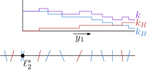
Figure 6: A snapshot of the sweepline (rotated to be horizontal), and the functions $k_{B}$, $k_{R}$, and $k$ expressing the number of outliers as a function of $y_{1}$.

The data structure.

We now argue we can maintain an efficient representation of the function $k$ in case $\ell_{2,y}^{*}=-\infty$. We then argue that we can also use the structure to query with other values of $\ell_{2}^{*}$. Our data structure is a fully persistent red-black tree [12] that stores the lines of $B^{*}\cup R^{*}$ in the order in which they intersect the vertical (sweep)line at $x$. We annotate each node $\nu$ with: (i) the number $k_{R}^{\nu}$ of red lines in its subtree, (ii) the number $k_{B}^{\nu}$ of blue lines in its subtree, (iii) the minimum value $\min^{\nu}$ of $k(y_{1})$ when restricted to all lines in the subtree rooted at $\nu$, and (iv) the value $\hat{y}^{\nu}$ achieving that minimum. Let $\ell$ and $r$ be the children of $\nu$, and observe that $\min^{\nu}=\min\{\min^{\ell}+k_{B}^{r},\min^{r}+k_{R}^{\ell}\}$. Hence, $\min^{\nu}$ can be (re)computed from the values of its children. The same applies for $k_{R}^{\nu}$ and $k_{B}^{\nu}$. Therefore, we can easily support inserting or deleting a line in $O(\log n)$ time. Indeed, inserting a red line that intersects the vertical line at $x$ in $y$, increases the error either for all values $y^{\prime}>y$ or for all value $y^{\prime}<y$ by exactly one, hence this affects only $O(\log n)$ nodes in the tree.

Observe that for $\ell^{*}_{2,y}=-\infty$ the root $\nu$ of the tree stores the value $\min^{\nu}=\min_{y}k(y)$, and the value $\hat{y}^{\nu}$ attaining this minimum. Hence, for such queries we can report the answer in constant time. To support querying with a different value of $\ell^{*}_{2,y}$, we simply split the tree at $\ell^{*}_{2,y}$, and use the subtree storing the lines above $\ell^{*}_{2}$ to answer the query. Observe that the number of blue lines below $\ell_{2}^{*}=(x,y_{2})$ is a constant with respect to $y_{1}\geq y_{2}$. Hence, it does not affect the position at which $\min_{y>y_{2}}k(y)$ attains its minimum. Splitting the tree and then answering the query takes $O(\log n)$ time. After the query we discard the two subtrees and resume using the original one, which we still have access to as the tree is fully persistent. We thus obtain the following result:

Theorem 5.3.

Given two sets of $n$ points $B,R\subset\mathbb{R}^{2}$, we can compute a strip $\mathcal{W}_{B}$ minimizing the total number of outliers $k$ in $O(n^{2}\log n)$ time.

6 Separation with a wedge

We consider the case where the region $\mathcal{W}_{B}$ is a single wedge and $\mathcal{W}_{R}$ is the other three wedges. In Section 6.1 we show how to minimize $k_{R}$ in optimal $O(n\log n)$, and in Section 6.2 we show how to minimize $k_{B}$ in $O(n^{3}\log n)$.

6.1 Wedge separation with red outliers

We distinguish between $\mathcal{W}_{B}$ being an $\mathrm{East}$ or $\mathrm{West}$ wedge, and a $\mathrm{North}$ or $\mathrm{South}$ wedge. In either case we can compute optimal lines $\ell_{1}$ and $\ell_{2}$ defining $\mathcal{W}_{B}$ in $O(n\log n)$ time.

Finding an East or West wedge.

We wish to find two lines $\ell_{1}$ and $\ell_{2}$ such that $\mathcal{W}_{B}(\ell_{1},\ell_{2})=\mathrm{East}(\ell_{1},\ell_{2})$ or $\mathcal{W}_{B}(\ell_{1},\ell_{2})=\mathrm{West}(\ell_{1},\ell_{2})$, i.e. we wish to find $\ell_{1}$ and $\ell_{2}$ such that every blue point and as few red points as possible lie above $\ell_{1}$ and below $\ell_{2}$. In the dual this corresponds to two points $\ell_{1}^{*}$ and $\ell_{2}^{*}$ such that all blue lines and as few red lines as possible lie below $\ell_{1}^{*}$ and above $\ell_{2}^{*}$, as in Figure 7.

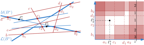
Figure 7: The arrangement of $B^{*}\cup R^{*}$ with its parameter space and forbidden regions.

Clearly $\ell_{1}^{*}$ must lie above $\mathcal{U}(B^{*})$, and $\ell_{2}^{*}$ below $\mathcal{L}(B^{*})$, and by Lemma 3.3 we can even assume they lie on $\mathcal{U}(B^{*})$ and $\mathcal{L}(B^{*})$. Similar to the case of strips in Section 5.1, we parameterize $\mathcal{U}(B^{*})$ and $\mathcal{L}(B^{*})$ over $\mathbb{R}^{2}$ such that a point $(p,q)$ in this parameter space corresponds to two dual points $\ell_{1}^{*}$ and $\ell_{2}^{*}$, with $\ell_{1}^{*}$ on $\mathcal{U}(B^{*})$ at $x=p$ and $\ell_{2}^{*}(y)$ on $\mathcal{L}(B^{*})$ at $x=q$, as illustrated in Figure 7. We wish to find a value in our parameter space whose corresponding segment minimizes the number of red misclassifications. Let the forbidden regions of a red line $r$ be those regions in the parameter space in which corresponding segments misclassify $r$. We distinguish between five types of red lines, as in Figure 7 (left):

• Line $a$ intersects $\mathcal{U}(B^{*})$ in points $a_{1}$ and $a_{2}$, with $a_{1}$ left of $a_{2}$. Only segments with $\ell_{1}^{*}$ left of $a_{1}$ or right of $a_{2}$ misclassify $a$. This produces two forbidden regions: $(-\infty,a_{1})\times(-\infty,\infty)$ and $(a_{2},\infty)\times(-\infty,\infty)$.

• Line $b$ intersects $\mathcal{L}(B^{*})$ in points $b_{1}$ and $b_{2}$, with $b_{1}$ left of $b_{2}$. Symmetric to line $a$ this produces forbidden regions $(-\infty,\infty)\times(-\infty,b_{1})$ and $(-\infty,\infty)\times(b_{2},\infty)$.

• Line $c$ intersects $\mathcal{U}(B^{*})$ in $c_{1}$ and $\mathcal{L}(B^{*})$ in $c_{2}$, with $c_{1}$ left of $c_{2}$. Only segments with endpoints after $c_{1}$ and before $c_{2}$ misclassify $c$. This produces the region $(c_{1},\infty)\times(-\infty,c_{2})$.

• Line $d$ intersects $\mathcal{U}(B^{*})$ in $d_{1}$ and $\mathcal{L}(B^{*})$ in $d_{2}$, with $d_{1}$ right of $d_{2}$. Symmetric to line $c$ it produces the forbidden region $(-\infty,d_{1})\times(d_{2},\infty)$.

• Line $e$ intersects neither $\mathcal{U}(B^{*})$ nor $\mathcal{L}(B^{*})$. All segments misclassify $e$. In the primal this corresponds to red points inside the blue convex hull. This produces one forbidden region; the entire plane $\mathbb{R}^{2}$.

As in Section 6.1, the above list is exhaustive.

The forbidden regions generated by the red lines $r^{*}\in R^{*}$ divide the parameter space in axis-aligned orthogonal regions. Our goal is again to find a point with minimum ply in these forbidden regions. For this we prove the following lemma:

Lemma 6.1.

Given a set $\mathcal{R}$ of $n$ constant complexity, axis-aligned, orthogonal regions, we can compute the point with minimum ply in $O(n\log n)$ time.

Proof 6.2.

We sweep through the plane with a vertical line $z$ while maintaining a minimum ply point on $z$. See Figure 7 for an illustration. As a preprocessing step, we cut each region into a constant number of axis-aligned (possibly unbounded) rectangles, and build the skeleton of a segment tree on the $y$-coordinates of the vertical sides of these rectangles in $O(n\log n)$ time [11]. This results in a binary tree with a leaf for each elementary $x$-interval induced by the segments. A node $v$ corresponds to the union of the intervals of its children. The canonical subset of $v$ is the set of intervals containing $v$ but not the parent of $v$. For a node $v$ we store the size $s(v)$ of its canonical subset, the minimum ply $\mathrm{ply}(v)$ within the subtree of $v$, and a point attaining this minimum ply.

We start with $z$ at $-\infty$ and sweep to the right. When we encounter the left (respectively right) side of a rectangle with vertical segment $I=(y_{1},y_{2})$, insert (respectively delete) $I$ in the segment tree. Since we already constructed the skeleton of this tree, the endpoints of $I$ are already present, so the shape of the tree does not change. Updating $s(v)$ takes $O(\log n)$ time [11], since $I$ is in the canonical subset of only $O(\log n)$ nodes. The minimum ply in a node $v$ with children $c_{1},c_{2}$, and a point attaining this minimum, can be updated simultaneously: $\mathrm{ply}(v)=s(v)+\min(\mathrm{ply}(c_{1}),\mathrm{ply}(c_{2}))$. After every update, the root node stores the current minimum ply. We maintain and return the overall minimum ply over all positions of the sweepline.

Since there are $O(n)$ rectangles, each of which is added and removed once in $O(\log n)$ time, this leads to a running time of $O(n\log n)$.

We construct $\mathcal{U}(B^{*})$ and $\mathcal{L}(B^{*})$ in $O(n\log n)$ time. For every red line $r$, we calculate its intersections with $\mathcal{U}(B^{*})$ and $\mathcal{L}(B^{*})$ in $O(\log n)$ time, determine its type ($a-e$), and construct its forbidden regions. By Lemma 6.1 we can find a point with minimum ply in these forbidden regions in $O(n\log n)$ time.

Theorem 6.3.

Given two sets of $n$ points $B,R\subset\mathbb{R}^{2}$, we can construct an $\mathrm{East}$ or $\mathrm{West}$ wedge containing all points of $B$ and the fewest points of $R$ in $O(n\log n)$ time.

Finding a South or North wedge

We wish to find two lines $\ell_{1}$ and $\ell_{2}$ such that $\mathcal{W}_{B}(\ell_{1},\ell_{2})=\mathrm{South}(\ell_{1},\ell_{2})$, i.e. such that every blue point and as few red points as possible lie below both $\ell_{1}$ and $\ell_{2}$. The case where $\mathcal{W}_{B}(\ell_{1},\ell_{2})=\mathrm{North}(\ell_{1},\ell_{2})$ is symmetric. In the dual this corresponds to two points $\ell_{1}^{*}$ and $\ell_{2}^{*}$ such that all blue lines and as few red lines as possible lie above both $\ell_{1}^{*}$ and $\ell_{2}^{*}$.

Clearly both $\ell_{1}^{*}$ and $\ell_{2}^{*}$ must lie below $\mathcal{L}(B^{*})$, and by Lemma 1 we can even assume they lie on $\mathcal{L}(B^{*})$. Similar to before we parameterize the $x$-coordinate of both points over $\mathbb{R}^{2}$, such that a point $(p,q)$ in the parameter space corresponds to two dual points $\ell_{1}^{*}$ and $\ell_{2}^{*}$, with $\ell_{1}^{*}$ on $\mathcal{L}(B^{*})$ at $x=p$ and $\ell_{2}^{*}$ on $\mathcal{L}(B^{*})$ at $x=q$. Note that the resulting parameter space $P$ is symmetric over $y=x$, since $\ell_{1}^{*}$ and $\ell_{2}^{*}$ are interchangeable.

Let $s_{\min}$ ($s_{\max}$) be the minimum (maximum) slope of all blue lines. There are now four types of red lines, as illustrated in Figure 8:

• line $a$: intersects $\mathcal{L}(B^{*})$ twice in $a_{1}$ and $a_{2}$. Line $a$ is misclassified if both $\ell_{1}^{*}$ and $\ell_{2}^{*}$ lie below $a$. In the parameter space, this corresponds to four forbidden corners of the parameter space, as in Figure 8.

• line $b$: intersects $\mathcal{L}(B^{*})$ once in $b_{1}$ and has a slope $s\in(-\infty,s_{\min})$. Only segments with both endpoints left of $b_{1}$ misclassify $b$, producing a forbidden bottomleft quadrant in the parameter space $P$.

• line $c$: intersects $\mathcal{L}(B^{*})$ once in $c_{1}$ and has a slope $s\in(s_{\max},\infty)$. Similar to $b$, this produces a forbidden topright quadrant.

• line $d$: does not intersect $\mathcal{L}(B^{*})$. This point will always be misclassified by a $\mathrm{North}$ wedge. In the primal, this corresponds to red points lying in or directly below the convex hull of the blue points.

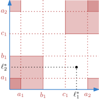
Figure 8: Left: The arrangement of lines $B^{*}$ and $R^{*}$. Right: The corresponding parameter space $P$ and forbidden regions.

As before we construct all forbidden regions, and apply the algorithm of Lemma 6.1 to obtain a point in the parameter space with minimum ply in $O(n\log n)$ time. We obtain the following:

Theorem 6.4.

Given two sets of $n$ points $B,R\subset\mathbb{R}^{2}$, we can construct a $\mathrm{North}$ or $\mathrm{South}$ wedge containing all points of $B$ and the fewest points of $R$ in $O(n\log n)$ time.

6.2 Wedge separation with blue outliers

We now consider the case where all red points must be classified correctly, and we minimize the number of blue outliers. We present an $O(n^{3}\log n)$ time algorithm to this end. The main idea is once again to map blue points $b$ to a region $I_{b}$ in some solution space corresponding to wedges that misclassify $b$. However, contrary to the other sections we will obtain this mapping directly from the primal space.

By Lemma 3.3, there exists an optimal wedge $\mathcal{W}_{B}(\ell_{1},\ell_{2})$ in which $\ell_{1}$ and $\ell_{2}$ both go through a blue and a red point. Consider the case $\mathcal{W}_{B}(\ell_{1},\ell_{2})$ is an $\mathrm{East}$ wedge (the other cases, including the cases where it is a $\mathrm{North}$ or $\mathrm{South}$ wedge, are symmetric). Fix a line $\ell_{2}$ going through a blue and a red point, and assume that $\ell_{2}$ has a greater slope than $\ell_{1}$. That means all points above $\ell_{2}$ are outside the wedge, so we only have to consider only the points below $\ell_{2}$.

Let $B^{\prime}$ and $R^{\prime}$ be the subset of blue, respectively red, points below $\ell_{2}$. Given a point $p$ on $\ell_{2}$, let $\ell_{1}(p)$ be the line through $p$ tangent to the upper half of $\mathit{CH}(R^{\prime})$, such that $R^{\prime}$ is just below the $\mathrm{East}$ wedge $\mathcal{W}_{B}(\ell_{1}(p),\ell_{2})$ (see Figure 9 for an illustration).

Lemma 6.5.

Given a line $\ell_{2}$ and a point $p\in\ell_{2}$, line $\ell_{1}(p)$ is an optimal line through $p$, i.e., there exists no better line $m$ through $p$ s.t. $|\mathcal{E}(m,\ell_{2})|<|\mathcal{E}(\ell_{1}(p),\ell_{2})|$.

Proof 6.6.

Assume there does exist a better line $m$. Since $m$ still correctly classifies all points in $R$, the line $\ell_{1}(p)$ has a slope at most as large as $m$, hence the wedge $\mathcal{W}_{B}(\ell_{1}(p),\ell_{2})$ contains the wedge $\mathcal{W}_{B}(m,\ell_{2})$. Therefore, wedge $\mathcal{W}_{B}(\ell_{1}(p),\ell_{2})$ contains at least as many blue points as wedge $\mathcal{W}_{B}(m,\ell_{2})$, while both correctly classify all red points. Thus, $|\mathcal{E}(m,\ell_{2})|\geq|\mathcal{E}(\ell_{1}(p),\ell_{2})|$, which contradicts our assumption that $m$ was better than $\ell_{1}(p)$. Therefore, such a better line $m$ does not exist.

We parameterize $\ell_{2}$ over $\mathbb{R}$ by $x$-coordinate such that each point $z\in\mathbb{R}$ corresponds to the wedge $\mathcal{W}_{B}(\ell_{1}(p),\ell_{2})$ with $p$ on the line $x=z$. Each blue point $b\in B^{\prime}$ defines a (possibly unbounded) forbidden region $I_{b}\subset\mathbb{R}$, such that $p\in I_{b}$ if and only if $\mathcal{W}_{B}(\ell_{1}(p),\ell_{2})$ does not contain $b$. More precisely, consider the tangents of $b$ with $\mathit{CH}(R^{\prime})$. These tangents define four wedges. Let $W_{1}$ be the wedge with bounded, non-empty intersection with $\ell_{2}$, and let $W_{2}$, $W_{3}$ and $W_{4}$ be the other wedges in clockwise order. The interval $I_{b}$ depends on which of the four wedges contains $\mathit{CH}(R^{\prime})$. For some segment $e$, let $x(e)$ be the set of $x$-coordinates of the points on $e$. We have the following four cases:

1. If $\mathit{CH}(R^{\prime})\subset W_{1}$, then $I_{b}=x(\ell_{2}\setminus W_{2})$ (Figure 9a).

2. If $\mathit{CH}(R^{\prime})\subset W_{2}$, then $I_{b}=x(\ell_{2}\setminus W_{3})=\mathbb{R}$ (Figure 9b).

3. If $\mathit{CH}(R^{\prime})\subset W_{3}$, then $I_{b}=x(\ell_{2}\setminus W_{4})$ (Figure 9c).

4. If $\mathit{CH}(R^{\prime})\subset W_{4}$, then $I_{b}=x(\ell_{2}\setminus W_{1})$ (Figure 9d).

Figure 9: The four different types of blue points and their regions $I_{b}$.

Any optimal line $\ell_{1}(p)$ corresponds to a point with minimum ply with respect to the regions $I_{b}$. Given these $O(n)$ regions, each being the union of at most two intervals, we can compute such a point in $O(n\log n)$ time by sorting and scanning the intervals. Computing the intervals takes $O(n\log n)$ time as well (by constructing $\mathit{CH}(R^{\prime})$ and finding the tangents of each blue point). This gives an optimal line $\ell_{1}(p)$ given $\ell_{2}$ in $O(n\log n)$ time. There are $O(n^{2})$ choices for the line $\ell_{2}$, and we simply try them all, obtaining the following result:

Theorem 6.7.

Given two sets of $n$ points $B,R\subset\mathbb{R}^{2}$, we can construct a wedge $\mathcal{W}_{B}$ minimizing the number of blue outliers $k_{B}$ in $O(n^{3}\log n)$ time.

7 Separation with a double wedge

In this section we present algorithms for double wedge classification with either red or blue outliers, where we make the assumption that the blue points (are supposed to) lie in a bowtie double wedge. We present an $O(n^{2})$ time algorithm for the case of red outliers in Section 7.1. In Section 7.2 we present a slightly slower $O(n^{2}\log n)$ time algorithm for the case of blue outliers. We handle the other cases (when $\mathcal{W}_{B}$ is an hourglass type wedge) through recoloring. Note that this causes the type of outliers to switch, and thus we end up with an $O(n^{2}\log n)$ time algorithm minimizing either $k_{B}$ or $k_{R}$.

7.1 Bowtie wedge separation with red outliers

We work in dual space, where a bowtie wedge containing all of $B$ dualizes to a line segment intersecting all lines of $B^{*}$. Any line of $R^{*}$ that is also intersected corresponds to a red point in the double wedge, which is an outlier. Hence we focus on computing a segment that intersects all lines of $B^{*}$ and as few of $R^{*}$ as possible.

Observe that the only segments intersecting all lines of $B^{*}$ have their endpoints in antipodal outer faces of $\mathcal{A}(B^{*})$. We can construct the outer faces in $O(n\log n)$ time [21], since the outer faces are the zone of the boundary of a sufficiently large rectangle (one that contains all vertices of the arrangement). With the outer faces constructed, we can apply a very similar algorithm to the one in Section 6.1 on each pair of antipodal faces (where for the parameter space, lines of type $c$ and $d$ add two forbidden quadrants rather than one). This gives an $O(n^{2}\log n)$ time algorithm for bowtie double wedge classification with red outliers.

Considering the running time is super-quadratic, we opt to construct the entire arrangement $\mathcal{A}(B^{*}\cup R^{*})$ of all lines explicitly. This takes $O(n^{2})$ time (see e.g. [11]), and as we show next, allows us to shave off a logarithmic factor.

Let $P,Q$ be the boundary chains of a pair of antipodal outer faces of $\mathcal{A}(B^{*})$, made up of a total of $m$ edges. We assume for ease of exposition that $P$ and $Q$ are separated by the $x$-axis, with $P$ above and $Q$ below the axis. We distinguish between two types of red lines: splitting lines and stabbing lines. Splitting lines intersect both $P$ and $Q$, while stabbing lines intersect at most one of $P$ and $Q$. Note that a line is a splitting line for exactly one pair of antipodal faces, but can be a stabbing line for multiple pairs of antipodal faces. For two points $p$ and $q$, let $\mathrm{stab}(p,q)$ (respectively $\mathrm{split}(p,q)$) be the number of stabbing (respectively splitting) lines that $\overline{pq}$ intersects. Let $s$ be the number of splitting lines for the pair of faces $P,Q$.

Lemma 7.1.

We can construct a line segment with endpoints on $P$ and $Q$ that intersects as few red lines as possible in $O(s^{2}+m+n)$ time.

Proof 7.2.

See Figure 10 for an illustration. The $s$ splitting lines partition $P$ and $Q$ into $s+1$ chains each. Let $P_{0},\dots,P_{s}$ be the chains partitioning $P$ and let $Q_{0},\dots,Q_{s}$ be the chains partitioning $Q$, both in clockwise order along $P$ and $Q$. Consider some pair of chains $P_{i},Q_{j}$. Note that all segments starting in $P_{i}$ and ending in $Q_{j}$ intersect the same number of splitting lines, i.e. $\forall p_{1},p_{2}\in P_{i},\forall q_{1},q_{2}\in Q_{j}:\mathrm{split}(p_{1},q_{1})=\mathrm{split}(p_{2},q_{2})=\mathrm{split}(P_{i},Q_{j})$. Therefore the best segment from $P_{i}$ to $Q_{j}$ is the one that intersects the fewest stabbing lines. For points $p\in P_{i},q\in Q_{j}$, let $x_{p}$ be the number of stabbing lines above $p$, and $y_{q}$ the number of stabbing lines below $q$, and note that $\mathrm{stab}(p,q)=n-s-x_{p}-y_{q}$. Thus, the best segment from $P_{i}$ to $Q_{j}$ is $\overline{p_{i}q_{j}}$, where $p_{i}=\mathrm{argmax}_{p\in P_{i}}x_{p}$, and $q_{j}=\mathrm{argmax}_{q\in Q_{j}}y_{q}$. Note that $p_{i}$ does not depend on $Q_{j}$, and vice versa.

We compute these points $p_{i}$ for all chains $P_{i}$ (and symmetrically $q_{j}$ for all chains $Q_{j}$) as follows. We move a point $p$ clockwise along $P$ in the arrangement $\mathcal{A}(B^{*}\cup R^{*})$, maintaining $x_{p}$, as well as $p_{\max}$ and $x_{p_{\max}}$, the (point attaining the) maximum value of $x_{p}$ encountered so far on the current chain $P_{i}$. When we cross a stabbing line $\ell$ we increment or decrement $x_{p}$, depending on the slope of $\ell$. Specifically, if the slope of $\ell$ is greater than the slope of the edge of $P$ we are currently on then we decrement $x_{p}$, and otherwise we increment the count. When we reach the end of chain $P_{i}$, i.e. when we cross a splitting line or reach the end of $P$, we set $p_{i}=p_{\max}$, and reset $p_{\max}$ and $x_{p_{\max}}$. This procedure takes $O(m+n)$ time.

For each segment $\overline{p_{i}q_{j}}$, we now know $\mathrm{stab}(p_{i},q_{j})=n-s-x_{p_{i}}-y_{q_{j}}$. Next we show that we can compute the number of splitting lines $\mathrm{split}(P_{i},Q_{j})$ intersected by segments with endpoints on $P_{i}$ and $Q_{j}$, for all pairs, in $O(s^{2})$ time. For this we use dynamic programming. Let $\ell_{i}$ be the splitting line in between chain $P_{i}$ and $P_{i+1}$. We compute the number of splitting lines $\mathrm{split}(P_{i},Q_{i})$ between each pair of chains with the following recurrence (recall that the partitionings of $P$ and $Q$ are in clockwise order):

$$\mathrm{split}(P_{i},Q_{j}) =\begin{cases}s-j&\text{if $i=0$,}\\ \mathrm{split}(P_{i-1},Q_{j})+1&\text{if segment $\overline{p_{i}q_{j}}$ intersects $\ell_{i-1}$,}\\ \mathrm{split}(P_{i-1},Q_{j})-1&\text{if segment $\overline{p_{i}q_{j}}$ does not intersect $\ell_{i-1}$.}\end{cases}$$

We compute the $O(s^{2})$ values for $\mathrm{split}(P_{i},Q_{j})$ in $O(s^{2})$ time with dynamic programming. Having computed both $\mathrm{stab}(p_{i},q_{j})$ and $\mathrm{split}(P_{i},Q_{j})$ for all pairs of chains, we compute the pair minimizing $\mathrm{stab}(p_{i},q_{j})+\mathrm{split}(P_{i},Q_{j})$ in $O(s^{2})$ additional time by iterating through them. The segment connecting this pair intersects the fewest red lines.

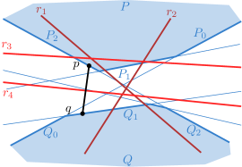
Figure 10: Two antipodal faces $P$ and $Q$, with two splitting lines $r_{1},r_{2}$ and two stabbing lines $r_{3},r_{4}$, and an optimal segment $\overline{pq}$ from $P$ to $Q$.

There are $O(n)$ pairs of antipodal blue faces $P$ and $Q$. For the $x^{\mathrm{th}}$ pair, let $m_{x}$ be their total complexity and $s_{x}$ be the number of splitting lines. We apply the above algorithm to each pair, leading to total time $O(\sum_{x}(s_{x}^{2}+m_{x}+n))$. The total complexity of all outer faces is $O(n)$, and a red line is a splitting line for exactly one pair of antipodal faces. Hence the total running time simplifies to $O(n^{2})$.

Theorem 7.3.

Given two sets of $n$ points $B,R\subset\mathbb{R}^{2}$, we can construct the bowtie double wedge $\mathcal{W}_{B}$ minimizing the number of red outliers $k_{R}$ in $O(n^{2})$ time.

7.2 Bowtie wedge separation with blue outliers

Again we work in dual space, where a bowtie double wedge $\mathcal{W}_{B}$ containing some of $B$ and none of $R$ dualizes to a line segment intersecting some lines of $B^{*}$ and none of $R^{*}$. Any line of $B^{*}$ that is not intersected corresponds to a blue point not in $\mathcal{W}_{B}$, which is an outlier. Hence we focus on computing a segment that intersects the most lines of $B^{*}$, while intersecting none of $R^{*}$.

Observe that the only segments intersecting no line of $R^{*}$ lie completely inside a face of $\mathcal{A}(R^{*})$. We construct the arrangements $\mathcal{A}(R^{*})$ and $\mathcal{A}(B^{*}\cup R^{*})$ in $O(n^{2})$ time [11].

Consider a face $F$ of $\mathcal{A}(R^{*})$. We wish to compute the segment in $F$ that intersects the most blue lines, and which hence has the fewest blue outliers of any segment in $F$. W.l.o.g. we only consider segments with endpoints on the boundary $P$ of $F$, since we can always extend a segment without introducing blue misclassifications.

Let $B^{*}_{P}$ be the set of blue lines intersecting $P$, which we report by scanning over $P$ inside the arrangement $\mathcal{A}(B^{*}\cup R^{*})$. This takes $O(|P|+|B^{*}_{P}|)$ time. We reuse the parameter space tool from Section 6.1. Fix an arbitrary point $o$ on $P$ and parameterize over $P$ in clockwise order, with $P(0)=P(1)=o$. For a given blue line $b$ intersecting $P$ in points $P(b_{1}),P(b_{2})$ with $b_{1}<b_{2}$, a segment $\overline{P(\ell_{1}^{*})P(\ell_{2}^{*})}$ intersects $b$ if and only if $\ell_{1}^{*}\in[b_{1},b_{2}]$ and $\ell_{2}^{*}\in[0,b_{1}]\cup[b_{2},1]$, or $\ell_{1}^{*}\in[0,b_{1}]\cup[bPs_{2},1]$ and $\ell_{2}^{*}\in[b_{1},b_{2}]$. This results in four forbidden regions in the parameter space, as in Figure 11.

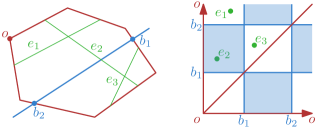
Figure 11: A face $F$ with its parameter space and the forbidden regions induced by the blue line.

We compute the intersection values $x_{1},x_{2}$ for all lines in $B^{*}_{P}$ by scanning over $P$ in $\mathcal{A}(B^{*}\cup R^{*})$, as we did for reporting all lines in $B^{*}_{P}$. The segment $\overline{P(\ell_{1}^{*})P(\ell_{2}^{*})}$ intersecting the most blue lines corresponds to the point $(\ell_{1}^{*},\ell_{2}^{*})$ in the parameter space with maximum ply. Similar to Lemma 6.1, where we compute the minimum ply point in a set of rectangles, we can compute the maximum ply point in this set of $|B^{*}_{P}|$ rectangles in $O(|B^{*}_{P}|\log|B^{*}_{P}|)$ time.

The total complexity of the sets $B^{*}_{P}$, over all faces of $\mathcal{A}(R^{*})$, is at most the complexity of $\mathcal{A}(B^{*}\cup R^{*})$, that is $O(n^{2})$. We therefore obtain a total running time of $O(n^{2}\log n)$.

Theorem 7.4.

Given two sets of $n$ points $B,R\subset\mathbb{R}^{2}$, we can construct a bowtie double wedge $\mathcal{W}_{B}$ minimizing the number of blue outliers $k_{B}$ in $O(n^{2}\log n)$ time.

8 Concluding Remarks

We presented efficient algorithms for robust bichromatic classification of $R\cup B$ with at most two lines. Our results depend on the shape of the region containing (most of the) blue points $B$, and whether we wish to minimize the number of red outliers, blue outliers, or both. See Table 1. Many of our algorithms reduce to the problem of computing a point with minimum ply with respect to a set of regions. We can extend these algorithms to support weighted regions, and thus we may support classifying weighted points (minimizing the weight of the misclassified points). It is interesting to see if we can support other error measures as well.

There are also still many open questions. The most prominent questions are wheter we can design faster algorithms for the algorithms minimizing the total number of outliers $k$, in particular for the wedge and double wedge case. For the strip case, the running time of our algorithm $O(n^{2}\log n)$ matches the worst case running time for halfplanes ($O((n+k^{2})\log n)$, which is $O(n^{2}\log n)$ when $k=O(n)$), but it would be interesting to see if we can also obtain algorithms sensitive to the number of outliers $k$. Furthermore, it would be interesting to establish lower bounds for the various problems. In particular, are our algorithms for computing a halfplane minimizing $k_{R}$ optimal, and in case of wedges (where the problem is asymmetric) is minimizing the number of blue outliers $k_{B}$ really more difficult then minimizing $k_{R}$?

References

- [1] Charu C. Aggarwal. Data classification: algorithms and applications. CRC press, 2014.
- [2] Carlos Alegría, David Orden, Carlos Seara, and Jorge Urrutia. Separating bichromatic point sets in the plane by restricted orientation convex hulls. Journal of Global Optimization, 85(4):1003–1036, 2023. doi:10.1007/s10898-022-01238-9.
- [3] Edoardo Amaldi and Viggo Kann. The complexity and approximability of finding maximum feasible subsystems of linear relations. Theoretical Computer Science, 147(1&2):181–210, 1995. doi:10.1016/0304-3975(94)00254-G.
- [4] Esther M. Arkin, Delia Garijo, Alberto Márquez, Joseph S. B. Mitchell, and Carlos Seara. Separability of point sets by k-level linear classification trees. International Journal of Computational Geometry & Applications, 22(2):143–166, 2012. doi:10.1142/S0218195912500021.
- [5] Esther M. Arkin, Ferran Hurtado, Joseph S. B. Mitchell, Carlos Seara, and Steven Skiena. Some lower bounds on geometric separability problems. International Journal of Computational Geometry & Applications, 16(1):1–26, 2006. doi:10.1142/S0218195906001902.
- [6] Bogdan Armaselu and Ovidiu Daescu. Dynamic minimum bichromatic separating circle. Theoretical Computer Science, 774:133–142, 2019. doi:10.1016/j.tcs.2016.11.036.
- [7] Boris Aronov, Delia Garijo, Yurai Núñez Rodríguez, David Rappaport, Carlos Seara, and Jorge Urrutia. Minimizing the error of linear separators on linearly inseparable data. Discrete Applied Mathematics, 160(10-11):1441–1452, 2012. doi:10.1016/j.dam.2012.03.009.
- [8] Daniel Bertschinger, Henry Förster, and Birgit Vogtenhuber. Intersections of double-wedge arrangements. In Proc. European Workshop on Computational Geometry (EuroCG 2022), pages 58–1, 2022.
- [9] Timothy M. Chan. Low-dimensional linear programming with violations. SIAM Journal on Computing, 34(4):879–893, 2005. doi:10.1137/S0097539703439404.
- [10] Corinna Cortes and Vladimir Vapnik. Support-vector networks. Machine Learning, 20(3):273–297, Sep 1995. doi:10.1007/BF00994018.
- [11] Mark de Berg, Otfried Cheong, Marc J. van Kreveld, and Mark H. Overmars. Computational geometry: algorithms and applications, 3rd Edition. Springer, 2008.
- [12] James R. Driscoll, Neil Sarnak, Daniel Dominic Sleator, and Robert Endre Tarjan. Making data structures persistent. Journal of Compututer and Systtem Sciences, 38(1):86–124, 1989. doi:10.1016/0022-0000(89)90034-2.
- [13] Sariel Har-Peled and Vladlen Koltun. Separability with outliers. In Proc. 16th International Symposium on Algorithms and Computation, volume 3827 of Lecture Notes in Computer Science, pages 28–39. Springer, 2005. doi:10.1007/11602613\_5.
- [14] Ferran Hurtado, Mercè Mora, Pedro A. Ramos, and Carlos Seara. Separability by two lines and by nearly straight polygonal chains. Discrete Applied Mathematics, 144(1-2):110–122, 2004. doi:10.1016/j.dam.2003.11.014.
- [15] Ferran Hurtado, Marc Noy, Pedro A. Ramos, and Carlos Seara. Separating objects in the plane by wedges and strips. Discrete Applied Mathematics, 109(1-2):109–138, 2001. doi:10.1016/S0166-218X(00)00230-4.
- [16] Ferran Hurtado, Carlos Seara, and Saurabh Sethia. Red-blue separability problems in 3D. International Journal of Computational Geometry & Applications, 15(2):167–192, 2005. doi:10.1142/S0218195905001646.
- [17] Nimrod Megiddo. Linear programming in linear time when the dimension is fixed. Journal of the ACM, 31(1):114–127, 1984. doi:10.1145/2422.322418.
- [18] D. Sculley and Gabriel M. Wachman. Relaxed online SVMs for spam filtering. In Proc. 30th Annual International ACM SIGIR Conference on Research and Development in Information Retrieval, SIGIR ’07, page 415–422. Association for Computing Machinery, 2007. doi:10.1145/1277741.1277813.
- [19] Carlos Seara. On geometric separability. PhD thesis, Univ. Politecnica de Catalunya, 2002.
- [20] Aihua Shen, Rencheng Tong, and Yaochen Deng. Application of classification models on credit card fraud detection. In Proc. 2007 International conference on service systems and service management, pages 1–4. IEEE, 2007.
- [21] Haitao Wang. A simple algorithm for computing the zone of a line in an arrangement of lines. In Proc. 5th Symposium on Simplicity in Algorithms, pages 79–86. SIAM, 2022. doi:10.1137/1.9781611977066.7.