Particle-Wise Higher-Order SPH Field Approximation for DVR

Abstract

When employing Direct Volume Rendering (DVR) for visualizing volumetric scalar fields, classification is generally performed on a piecewise constant or piecewise linear approximation of the field on a viewing ray. Smoothed Particle Hydrodynamics (SPH) data sets define volumetric scalar fields as the sum of individual particle contributions, at highly varying spatial resolution. We present an approach for approximating SPH scalar fields along viewing rays with piecewise polynomial functions of higher order. This is done by approximating each particle contribution individually and then efficiently summing the results, thus generating a higher-order representation of the field with a resolution adapting to the data resolution in the volume.

Keywords: Scientific Visualization, Ray Casting, Higher-Order Approximation, Volume Rendering, Scattered Data, SPH

1 INTRODUCTION

Introduced by Gingold and Monaghan [Gingold and Monaghan, 1977] and independently by Lucy [Lucy, 1977], Smoothed Particle Hydrodynamics (SPH) is a group of methods for simulating dynamic mechanical processes, typically fluid or gas flows but also solid mechanics. The objective matter is modeled by means of particles, each representing a small portion of a simulated substance and attributed a specific mass, density, and other physical measures.

These discrete and scattered particles define scalar and vector fields on the spatial continuum through an interpolation rule, determining a physical field as the sum of the isotropic contributions of the particles, each following a smooth function only of the distance from the particle position, called the kernel function. As an example, we refer to the SPH kernel function defined by the cubic B-spline [Rosswog, 2009]

$$\mathop{w}\mathopen{}\left(r\right)=\frac{1}{4\pi}\begin{cases}\left(2-r\right)^{3}-4\left(1-r\right)^{3},&0\leq r<1\\ \left(2-r\right)^{3},&1\leq r<2\\ 0,&2\leq r\;.\end{cases}$$ (1)

In this work, we assume the kernel function to have compact support. We consider this to be a minor restriction because kernel functions with compact support are appreciated in the SPH community for bounding the particles’ volumes of influence. Obviously, by simply defining some cut-off value as upper bound, any kernel function can be supported. Given such a function, a particle’s contribution to a scalar field can be expressed as

$$\frac{\mu\alpha}{\rho\zeta^{3}}\mathop{w}\mathopen{}\left(\frac{\left\|\boldsymbol{x}-\boldsymbol{\chi}\right\|}{\zeta}\right)$$

for the particle’s position $\boldsymbol{\chi}$, mass $\mu$, target field value $\alpha$, density $\rho$, and smoothing radius $\zeta$. While $\mu$, $\alpha$, and $\rho$ serve as simple multiplicative constants, defining only the amplitude of the contribution, $\zeta$ radially scales the domain and thus defines the radius of the particle’s volume of influence.

Direct Volume Rendering (DVR) has a long-standing tradition for visualizing scalar volumetric fields [Drebin et al., 1988] and is commonly implemented as a ray casting method. It builds on assigning visual characteristics, representing features of the field, to the target domain volume and then rendering it by casting viewing rays through the volume. The color of each pixel of the output image is the result of simulating the behavior of light traveling through the volume along a ray in opposite viewing direction.

Said visual characteristics, usually comprising light emission and absorption, are computed from local target field characteristics, like values or gradients, in a process called classification [Max, 1995]. It is commonly employed based on a piecewise constant or piecewise linear approximation of the target scalar field along the ray.

Direct volume rendering of astronomical SPH data was first performed by incorporating contributions of both grid and particle data into the optical model [Kähler et al., 2007]. Efficient full-featured DVR applied directly to large SPH data sets on commodity PC hardware has first been managed by resampling the scalar fields to a perspective grid held in a 3-d texture for each rendering frame [Fraedrich et al., 2010]. Later, DVR for large scattered data was proposed to be performed on the CPU by Knoll et al. [Knoll et al., 2014] and mostly applied to molecular dynamics. Although employing radial basis function kernel (RBF) interpolation similar to the SPH case, they focus on the very special task of rendering a surface defined by a density field. This is in line with more recent contributions in rendering SPH data, such as [Hochstetter et al., 2016] or [Oliveira and Paiva, 2022], targeting only simulated fluids.

The approaches for volume-rendering arbitrary SPH fields employ equidistant sampling of the target field along viewing rays and acting on a piecewise linear approximation of it, which, depending on the local particle density, may miss detailed features in regions of high particle density, or oversample particles with large smoothing length in sparse regions.

Thus, in this work, we explore the capabilities and limitations of approximating SPH scalar fields with higher-order piecewise polynomial functions, whose resolution adapts to the local resolution of the given particle data. The higher-order approximations may facilitate quantitatively more accurate output images at a worthwhile cost.

2 METHOD OVERVIEW

As SPH interpolation defines the target scalar field as the sum of particle contributions to it, our concept builds on approximating each individual particle contribution on a viewing ray and then employing the sum of these approximations. Although summing an indefinite number of piecewise polynomial functions may seem like a task of quadratic complexity not amenable to GPU processing, we encode these functions in a way reducing the summation to a simple sorting task.

Our method comprises three passes:

1. For each particle, approximate its contribution to all relevant viewing rays.

2. For each ray, sort the contribution data assigned to it with respect to the distance from the viewer.

3. For each ray, accumulate the contributions along the ray, classify and composite the result.

In the remainder of this section, we declare our concept of representing piecewise polynomial functions and show how these can be processed during the compositing sweep. In Section 3, we present a way to efficiently compute optimal approximations for single particle contributions during the first sweep. In Section 4, we then describe a pitfall that our higher-order approximation scheme involves and develop an improvement of our method to overcome this difficulty. Finally, in Section 5, we analyze the approximation errors implied by our scheme and discuss the choice of the major parameters like the approximation order, before concluding our work in Section 6.

Localized Difference Coefficients.

A real polynomial function $A:\mathbb{R}\to\mathbb{R}$ of order $D$ is generally represented by its coefficients, i. e., numbers $a_{d}\in\mathbb{R}$ such that $\mathop{A}\mathopen{}\left(t\right)=\sum_{d=0}^{D}a_{d}t^{d}$. They provide a direct image of how the function and all its derivatives behave at $t=0$ since the $d^{\text{th}}$ derivative of $A$ at $t=0$ amounts to $d!a_{d}$. If we wanted to know the value or derivative of order $d$ at some other $t_{*}$, we could compute it as

$$\mathop{A^{\left(d\right)}}\mathopen{}\left(t_{*}\right)=\sum_{j=d}^{D}\frac{j!}{\left(j-d\right)!}a_{j}t_{*}^{j-d}=d!\sum_{j=d}^{D}\binom{j}{d}a_{j}t_{*}^{j-d},$$

which shows that the real numbers

$$a_{*d}=\sum_{j=d}^{D}\binom{j}{d}a_{j}t_{*}^{j-d}$$

represent the order-$d$ behavior of $A$ at $t=t_{*}$ just as the $a_{d}$ do at $t=0$. In fact, $A$ can be expressed using these localized coefficients as

$$\mathop{A}\mathopen{}\left(t\right)=\sum_{d=0}^{D}a_{*d}\left(t-t_{*}\right)^{d}.$$

Now, a continuous piecewise polynomial function is defined by a sequence of border arguments $t_{0}<t_{1}<\dots$ and several polynomial functions $A_{0},A_{1},\dots$ such that each polynomial function $A_{k}$ is applied in its respective interval $\left[t_{k},t_{k+1}\right]$.

If we were representing each polynomial $A_{k}$ by its coefficients, summing several piecewise polynomial functions would require tracking the applicable polynomials for each resulting argument interval and summing their coefficients.

Instead, we save for each border argument $t_{k}$ the change that the overall function performs in all orders. Specifically, we save the localized coefficients of the difference between the polynomials $A_{k}$ applicable on the right of $t_{k}$ and $A_{k-1}$ applicable on its left.

Thus, when saving a piecewise polynomial approximation of order $D$ along a viewing ray, we encode it as a sequence of knots

$$\left(t_{k},\hat{a}_{k0},\dots,\hat{a}_{kD}\right),\quad k=0,1,\dots$$

consisting of a ray parameter $t_{k}$ defining the knot position on the ray and localized difference coefficients $\hat{a}_{k0},\dots,\hat{a}_{kD}$, such that

$$\mathop{A_{k}}\mathopen{}\left(t\right)-\mathop{A_{k-1}}\mathopen{}\left(t\right)=\sum_{d=0}^{D}\hat{a}_{kd}\left(t-t_{k}\right)^{d}.$$

Summing several piecewise polynomials encoded this way amounts to nothing more than sorting their joint knots for increasing knot positions. The resulting approximation can then be processed piece by piece, retrieving the localized coefficients $a_{k0},\dots,a_{kD}$ of each piece polynomial $A_{k}$ at its left boundary argument $t_{k}$ from the ones of the last piece according to the updating rule

$$a_{kd}=\hat{a}_{kd}+\sum_{j=d}^{D}\binom{j}{d}a_{\left(k-1\right)j}\left(t_{k}-t_{k-1}\right)^{j-d}$$ (2)

for $d=0,\dots,D$, which is a computation of constant complexity per piece, irrespective of the number of particles contributing.

3 APPROXIMATING SINGLE PARTICLE CONTRIBUTIONS

3.1 Deduction from Unit Particle

Since the same SPH kernel function is applied for all particles, their contributions to the volume differ in only a few scaling and translation parameters, namely their position $\boldsymbol{\chi}$, mass $\mu$, density $\rho$, smoothing radius $\zeta$, and applicable scalar field attribute $\alpha$.

Figure 1: Sketch of measures involved in the positional relationship between viewing ray and particle. The volume of influence of a particle with smoothing length $\zeta$ is intersected by a viewing ray, defined by base point $\boldsymbol{b}$ and unit direction vector $\boldsymbol{v}$. The particle’s contribution on the ray at a point $\mathop{\boldsymbol{x}}\mathopen{}\left(t\right)$ is determined by its distance to the particle position $\boldsymbol{\chi}$. We denote by $q$ the upper bound of the kernel function’s support, such that $q\zeta$ is the radius of the particle’s volume of influence.

To model a viewing ray, we fix a straight line with vector equation $\mathop{\boldsymbol{x}}\mathopen{}\left(t\right)=\boldsymbol{b}+t\boldsymbol{v}$ for some base point $\boldsymbol{b}\in\mathbb{R}^{3}$, unit direction vector $\boldsymbol{v}\in\mathbb{R}^{3}$, and parameter $t\in\mathbb{R}$. We consider a normalized particle, i. e., one of unit mass, unit density, unit field attribute, and unit smoothing radius. Assuming the base point $\boldsymbol{b}$ on the ray is the one closest to the particle position, the normalized particle’s contribution to this line is

$$\mathop{B_{\Lambda}}\mathopen{}\left(t\right)=\mathop{w}\mathopen{}\left(\sqrt{\Lambda^{2}+t^{2}}\right),$$

where $\Lambda$ is the distance between the particle’s position and the line. Then, the contribution of a specific data particle on a ray at distance $\Lambda\zeta$ from its position $\boldsymbol{\chi}$ amounts to

$$\frac{\mu\alpha}{\rho\zeta^{3}}\mathop{B_{\Lambda}}\mathopen{}\left(\frac{t-t_{\boldsymbol{\chi}}}{\zeta}\right),$$

where $t_{\boldsymbol{\chi}}$ is the parameter of the point on the ray closest to the particle position and $\Lambda=\frac{1}{\zeta}\left\|\boldsymbol{\chi}-\mathop{\boldsymbol{x}}\mathopen{}\left(t_{\boldsymbol{\chi}}\right)\right\|$. The situation is depicted in Figure 1.

Finding optimal piecewise polynomial approximations for $B_{\Lambda}$ for all $\Lambda$ within the SPH kernel’s support suffices to generate optimal approximations for any particle by just translating and scaling it in the same way. For quick access, we thus prepare a look-up table containing the localized difference coefficients of order-$D$ approximations of $B_{\Lambda}$ for many equidistant values of $\Lambda$. In the remainder of this section, we show how we can find these optimal approximations.

3.2 Optimization Problem Definition

Before we can find optimal approximations, we need to define what optimality shall mean in this context. Specifically, we have to settle on:

1. The space of eligible candidates, i. e., the condition of what we want to consider a feasible approximation.

2. The error measure defining whether one approximation is better than another.

The main restriction on the space of eligible approximation candidates is the imposition of a maximum polynomial degree $D$, i.e, the order of approximation, and the number $K$ of non-trivial polynomial pieces per particle, i. e., the number of non-zero polynomials defining the approximation of a single particle. We dedicate Section 5 to evaluating choices of $D$ and $K$ but leave them unspecified for now. Beyond that, we demand that our approximations shall be continuous and even functions with compact support. This seems reasonable, as our approximation target $B_{\Lambda}$ also has these properties.

For measuring the approximating quality of any piecewise polynomial function candidate $S:\mathbb{R}\to\mathbb{R}$, we apply its $L^{2}$ distance to $B_{\Lambda}$, i. e., we seek to minimize the approximation error

$$\mathop{E_{\Lambda}}\mathopen{}\left(S\right)=\left\|S-B_{\Lambda}\right\|_{2}=\left(\intop_{\mathbb{R}}\left[\mathop{S}\mathopen{}\left(t\right)-\mathop{B_{\Lambda}}\mathopen{}\left(t\right)\right]^{2}\mathop{}\!\mathrm{d}t\right)^{\frac{1}{2}}\!\!\!.$$ (3)

In contrast to the supremum norm, often used in approximation theory, this error measure punishes not only the maximum pointwise deviation from the target, but also the length of segments of high deviation. Moreover, another advantage of the $L^{2}$ norm is its associated inner product, which allows us to generate a closed-form solution of the optimal approximation and its error value as a function only of the knot positions, as shown in Section 3.3. We then find optimal knot positions through standard non-linear optimization as explained in Section 3.4.

3.3 Solution for Fixed Knot Positions

As a prerequisite for finding truly optimal approximations, we first handle the case of arbitrary fixed knot positions. Due to our evenness requirement, the negative knot positions are determined from the positive ones. Hence, our optimization domain is the set of even continuous piecewise polynomial functions with compact support, maximal degree $D$, maximal number of non-trivial pieces $K$, and positive knot positions $\theta_{1},\dots,\theta_{\left\lceil\nicefrac{{\vphantom{K}\smash{K}}}{{2}}\right\rceil}$. We denote this set by $\mathcal{S}$.

Consider the vector space $\mathop{L^{2}}\mathopen{}\left(\mathbb{R}\right)$ of square-integrable functions $\mathbb{R}\to\mathbb{R}$, which by the Riesz-Fischer theorem is complete with respect to the $L^{2}$ norm and therefore a Hilbert space when equipped with the inner product

$$\left\langle A,B\right\rangle=\intop_{\mathbb{R}}\mathop{A}\mathopen{}\left(t\right)\mathop{B}\mathopen{}\left(t\right)\mathop{}\!\mathrm{d}t\quad\text{for}\quad A,B\in\mathop{L^{2}}\mathopen{}\left(\mathbb{R}\right),$$

which induces the $L^{2}$ norm $\left\|A\right\|_{2}=\sqrt{\left\langle A,A\right\rangle}$. The approximation target $B_{\Lambda}$ is clearly an element of $\mathop{L^{2}}\mathopen{}\left(\mathbb{R}\right)$ as it is continuous and has compact support.

For any $A,B\in\mathop{L^{2}}\mathopen{}\left(\mathbb{R}\right)$, $B\not\equiv\mathbf{0}$, we denote by

$$\mathop{\operatorname{proj}_{B}}\mathopen{}\left(A\right)=\frac{\left\langle A,B\right\rangle}{\left\langle B,B\right\rangle}B$$

the orthogonal projection of $A$ on $B$.

As we will see shortly, $\mathcal{S}$ is a subspace of $\mathop{L^{2}}\mathopen{}\left(\mathbb{R}\right)$ of finite dimension $\left\lfloor\frac{KD}{2}\right\rfloor$, for which we can compute an orthogonal basis $\mathcal{A}$, which in turn we can use to calculate the orthogonal projection of $B_{\Lambda}$ on $\mathcal{S}$ as

$$S_{\Lambda}=\sum_{A\in\mathcal{A}}\mathop{\operatorname{proj}_{A}}\mathopen{}\left(B_{\Lambda}\right).$$ (4)

It is easy to show that $S_{\Lambda}$ is the unique error-optimal approximation of $B_{\Lambda}$ among the elements of $\mathcal{S}$ (proof in Appendix, Section 2). Therefore, all we need for computing the optimal approximation for fixed knot positions is a suitable orthogonal basis.

We specify a non-orthogonal basis as a starting point here: Let $\mathcal{J}$ be the set of pairs $\left(k,d\right)$ of positive integers $k\leq\left\lceil\nicefrac{{\vphantom{K}\smash{K}}}{{2}}\right\rceil$ and $d\leq D$ but excluding elements $\left(1,d\right)$ for uneven $d$ if $K$ is uneven. Then the set $\tilde{\mathcal{A}}=\left\{\vphantom{\big{\{}}\smash{\tilde{A}_{kd}}:\left(k,d\right)\in\mathcal{J}\right\}$ of functions

$$\mathop{\tilde{A}_{kd}}\mathopen{}\left(t\right)=\begin{cases}1&\text{if }\left|t\right|\leq\theta_{k-1}\\ 1-\left(\frac{\left|t\right|-\theta_{k-1}}{\theta_{k}-\theta_{k-1}}\right)^{d}&\text{if }\theta_{k-1}\leq\left|t\right|\leq\theta_{k}\\ 0&\text{if }\left|t\right|\geq\theta_{k}\end{cases}$$

is a basis of $\mathcal{S}$ (proof in Appendix, Section 1).

Given $\tilde{\mathcal{A}}$, we convert it into an orthogonal basis $\mathcal{A}=\left\{A_{kd}:\left(k,d\right)\in\mathcal{J}\right\}$ by employing the Gram-Schmidt process. Specifically, we recursively set

$$A_{k^{*}d^{*}}=\tilde{A}_{d^{*}k^{*}}-\sum_{\begin{subarray}{c}\left(k,d\right)\in\mathcal{J}\\ k<k^{*}\vee\left(k=k\wedge d<d^{*}\right)\end{subarray}}\mathop{\operatorname{proj}_{A_{kd}}}\mathopen{}\left(\vphantom{\big{(}}\smash{\tilde{A}_{d^{*}k^{*}}}\right)$$

in lexicographical order of pairs $\left(k^{*},d^{*}\right)\in\mathcal{J}$.

3.4 Optimal Knot Positions

While we can directly compute optimal approximations for given knot positions as shown above, finding error-optimal knot positions is a nonlinear optimization problem over the variables $\theta_{1},\dots,\theta_{\left\lceil\nicefrac{{\vphantom{K}\smash{K}}}{{2}}\right\rceil}$.

The objective function $E_{\Lambda}$ is continuous within the interior of the feasible domain defined by the constraints $0<\theta_{1}<\dots<\theta_{\left\lceil\nicefrac{{\vphantom{K}\smash{K}}}{{2}}\right\rceil}$, due to the continuity of the inner product and of the constructed basis with respect to the $\theta_{k}$, which would even hold for a discontinuous SPH kernel function. Also, we can expect to find a global optimizer within the interior of the feasible domain, i. e., without any of the constraints being active, because an equality of any two variables would be equivalent to a reduction of the number of non-zero pieces, diminishing the freedom for approximating and therefore resulting in higher or equal error. Hence, if a local optimum was attained at the feasible domain border, it could not be isolated because shifting one of the colliding $\theta_{k}$ and defining the polynomials on both of its sides to be equal would result in the same approximation function and therefore in the same error value.

While evaluating $E_{\Lambda}$ could be done following the steps above for every set of fixed $\theta_{1},\dots,\theta_{\left\lceil\nicefrac{{\vphantom{K}\smash{K}}}{{2}}\right\rceil}$, it is worthwhile to only fix $K$ and $D$ and perform the process in a symbolic manner, generating an explicit formula of the objective error function, which can later be evaluated for any knot positions and distance parameter $\Lambda$. The generation of a closed-form representation of an orthogonal basis for variable knot positions and $\Lambda$ has to be done only once as it does not depend on the SPH kernel used. However, the explicit expression of the approximation error following (4) requires closed-form solutions of the integrals defining the inner products $\left\langle A,B_{\Lambda}\right\rangle$ for orthogonal basis functions $A$. In the case of an SPH kernel defined by a continuous piecewise polynomial function such as the cubic B-spline kernel (1), this can clearly be achieved. In any case, as the symbolic computations are rather involved, computer algebra systems are of great help during this preparatory process.

We have conducted this process for the cubic B-spline kernel, going to considerable length to find a global optimizer for many discrete $\Lambda$. For $\Lambda$ close to the upper bound $q$, however, we have found the evaluation of some of the formulae to become instable. To obtain reliable results, we employed the GNU MPFR library to perform the computations in multiple precision arithmetic. Since we have not encountered any severe problems during these optimizations, we have reason to hope they are manageable for any piecewise polynomial SPH kernel function.

4 QUANTIZATION TO PREVENT HIGHER-ORDER ERRORS

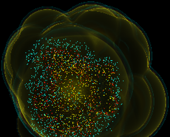
(a) (b) 

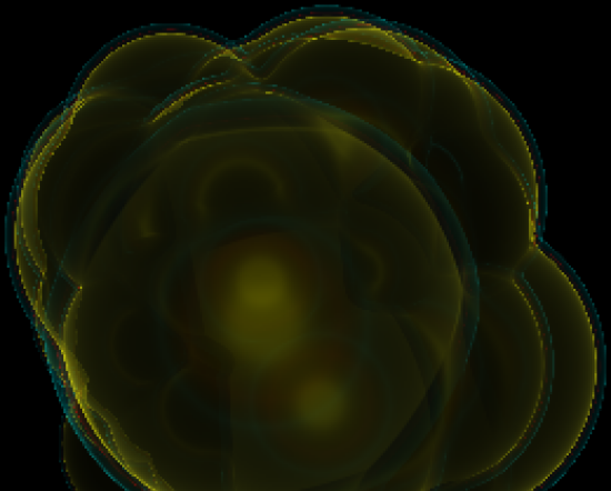
Figure 2: Extracts of sample renderings of the temperature field of an SPH data set using our higher-order SPH field approximation scheme and a transfer function emphasizing three rather low temperature value regions by mapping them to an emission of blue, yellow, and red light. All computations are performed in single precision on the GPU.
(a) clearly shows “sprinkling” artifacts caused by higher-order rounding error propagation, which “randomly” cause the field approximation on the ray to stay within one of the highlighted temperature regions far “behind” the particle cluster.
(b) shows the result of employing 10 slices of reinitialization to mitigate the problem.

4.1 Higher-order Rounding Error Propagation

For the stated efficiency reasons, the recursive computation of polynomial coefficients according to (2) is an integral component to our particle-wise approximation approach. However, it comes at a substantial price which may not be obvious at first glance. Directly applying (2) during the compositing sweep using floating-point numbers is problematic because rounding errors are propagated at higher order from front to back along the viewing ray, resulting in unreliable coefficients especially for higher $t$.

To illustrate the issue, consider a piecewise polynomial function modeling the contribution of a small number of particles. Clearly, the last piece polynomial of this approximation should be the zero polynomial. However at its starting knot, its value is most probably not computed to be zero but some value close to zero, due to rounding errors in the computation. Although this zeroth-order distortion may be negligible by itself, small rounding errors in higher-order terms cause large errors further down the ray. We may thus find the polynomial’s value to have grown far from zero for larger $t$.

The direct effect of these errors is an unstable result: When using a transfer function with focus on lower attribute values typically reached just before leaving the volumes of influence of the last contributing particles, the resulting pixel colors are highly unstable and the generated images show strong “sprinkling” artifacts, as shown in Figure 2 (a). Hence, solving this problem is indispensable if we want our higher-order ray casting concept to be of any use.

There are several conceivable measures for alleviation. One is to limit the maximum distance on the ray that the error may use to grow by introducing a number of special reinitialization knots at predetermined $t$ on all rays, as performed for the rendering of Figure 2 (b). When processing a particle during the first sweep, in addition to the knots encoding its higher-order approximation as difference coefficients, we also add to all covered reinitialization knots the localized coefficients of this particle’s contributions. Later when processing the sorted sequence of knots, whenever we encounter a reinitialization knot, we directly take the coefficients attached to it instead of computing the coefficients following the update rule (2), thus eliminating the effect of past errors for future pieces. However, this approach not only introduces the complexity of two different kinds of knots but also can only partially solve the problem. Besides, defining how many reinitialization knots to utilize is non-trivial.

Clearly, an alternative would be to avoid the cause of higher-order error propagation altogether and proceed to a direct, possibly localized, coefficient representation of the polynomials, considering for the computation of each result piece only the contributions with overlapping support. While this would most probably facilitate stable results, it would mean accepting the expense of determining for each piece the set of relevant contributions.

4.2 Exact Arithmetic Through Quantization

We propose yet another approach to fully avoid rounding errors during the computation of (2), namely by transferring all involved quantities from floating-point to fixed-point numbers, which allow an exact arithmetic. More precisely, we slightly shift all numbers encoding the individual contribution approximations into integer multiples of some quantum values, a process we call quantization. While this increases the approximation errors for the individual contributions, the update operations in (2) are reduced to exact integer manipulations.

Adhering to the notation used in (2), the values to be quantized are the elements of the knots $\left(t_{k},\hat{a}_{k0},\dots,\hat{a}_{kD}\right)$ and the localized coefficients $a_{kd}$. We thus seek to fix real quantum values $\tau>0$ and $\varsigma_{d}>0$ for $d=0,\dots,D$ such that $t_{k}\approx\bar{t}_{k}\tau$ for some $\bar{t}_{k}\in\mathbb{N}$ and $\hat{a}_{kd}\approx\bar{\hat{a}}_{kd}\varsigma_{d}$, $a_{kd}\approx\bar{a}_{kd}\varsigma_{d}$ for integers $\bar{\hat{a}}_{kd}$ and $\bar{a}_{kd}$. The quantized knots can then be encoded as the integer components $\left(\bar{t}_{k},\bar{\hat{a}}_{k0},\dots,\bar{\hat{a}}_{kD}\right)$.

Written in these terms, (2) becomes

$$\bar{a}_{kd}=\bar{\hat{a}}_{kd}+\sum_{j=d}^{D}\binom{j}{d}\frac{\varsigma_{j}\tau^{j-d}}{\varsigma_{d}}\bar{a}_{\left(k-1\right)j}\left(\bar{t}_{k}-\bar{t}_{k-1}\right)^{j-d},$$

which we have to guarantee to result in an integer for arbitrary integer values of previously computed $\left(\bar{t}_{k}-\bar{t}_{k-1}\right)$ and $\bar{a}_{\left(k-1\right)j}$. This can only be accomplished by requiring $\binom{j}{d}\frac{\varsigma_{j}\tau^{j-d}}{\varsigma_{d}}\in\mathbb{Z}$ for all $d$ and $j\geq d$, which we can fulfill by simply setting $\varsigma_{d}=\frac{\varsigma}{\tau^{d}}$ for all $d$, where we abbreviate $\varsigma=\varsigma_{0}$. This leaves us with only two quantum values: one length quantum $\tau$ and one field value quantum $\varsigma$. We show our strategy of choosing the two in Section 4.4.

However, we first specify in Section 4.3 how we set up the quantized knot positions $\bar{t}_{k}$ and difference coefficients $\bar{\hat{a}}_{kd}$, which later form the input of the coefficients update rule (2), now reduced to the integer-only representation

$$\bar{a}_{kd}=\bar{\hat{a}}_{kd}+\sum_{j=d}^{D}\binom{j}{d}\bar{a}_{\left(k-1\right)j}\left(\bar{t}_{k}-\bar{t}_{k-1}\right)^{j-d}.$$ (5)

4.3 Setting Quantized Knots

In order to not introduce higher-order errors through the back door after all, we have to ensure that the input to the integer computations does not contain such errors already. Each individual particle approximation has to have compact support, i. e., its knots have to exactly neutralize each other. This guides us to compute the knots of single particle contributions according to the following rules (derivation in Appendix, Section 3).

Given a particle with attributes $\mu$, $\rho$, $\zeta$, and $\alpha$, positioned at distance $\Lambda\zeta$ from the ray with closest point parameter $t_{\boldsymbol{\chi}}$, we select from the look-up table the optimal normalized positive knot positions $\theta_{k}$ and localized difference coefficients $\hat{s}_{kd}$ corresponding to the normalized distance closest to $\Lambda$, all in floating-point representation.

We then set the knot position quantum counts to

$$\bar{t}_{0}=\left\lceil\frac{t_{\boldsymbol{\chi}}}{\tau}\right\rfloor\text{ and }\;\bar{t}_{k}=\bar{t}_{0}+\left\lceil\frac{\zeta\theta_{k}}{\tau}\right\rfloor,\;\bar{t}_{-k}=2\bar{t}_{0}-\bar{t}_{k}$$

for $k=1,\dots,\left\lceil\nicefrac{{\vphantom{K}\smash{K}}}{{2}}\right\rceil$, where we use $\left\lceil\cdot\right\rfloor$, a notation inspired by [Hastad et al., 1989, page 860], to refer to just a usual nearest integer rounding function. In this context it is irrelevant whether we round $z+\frac{1}{2}$ to $z$ or to $z+1$ for $z\in\mathbb{Z}$.

Then, for $k\geq 1$, except for $k=1$ and uneven $d$ if $K$ is uneven, the quantized localized difference coefficients are computed as

$$\bar{\hat{a}}_{kd}=\left\lceil\frac{\tau^{d}\mu\alpha\hat{s}_{kd}}{\varsigma\rho\zeta^{d+3}}\right\rfloor\text{ and }\;\bar{\hat{a}}_{-kd}=\left(-1\right)^{d+1}\bar{\hat{a}}_{kd}.$$

In case of $K$ being even, there is a middle knot with possibly non-zero coefficients

$$\bar{\hat{a}}_{0d}=-2\sum_{k=-\left\lceil\nicefrac{{\vphantom{K}\smash{K}}}{{2}}\right\rceil}^{-1}\sum_{j=d}^{D}\binom{j}{d}\bar{\hat{a}}_{kj}\left(\bar{t}_{0}-\bar{t}_{k}\right)^{j-d}$$

for uneven $d$. Otherwise, there is no middle knot, i. e., $\bar{\hat{a}}_{0d}=0$ for all $d$, but we set

$$\bar{\hat{a}}_{-1d}=-\!\!\!\!\sum_{k=-\left\lceil\nicefrac{{\vphantom{K}\smash{K}}}{{2}}\right\rceil}^{-2}\!\!\!\bar{\hat{a}}_{kd}-\!\!\!\sum_{j=d+1}^{D}\!\binom{\!j}{d\!}\!\sum_{k=-\left\lceil\nicefrac{{\vphantom{K}\smash{K}}}{{2}}\right\rceil}^{-1}\!\!\!\bar{\hat{a}}_{kj}\left(\bar{t}_{0}-\bar{t}_{k}\right)^{j-d}$$

and $\bar{\hat{a}}_{1d}=\left(-1\right)^{d+1}\bar{\hat{a}}_{-1d}$ in descending order of uneven $d$.

4.4 Specifying Quantum Values

Computing optimal quantum values requires the definition of a manageable error measure for minimization. In our attempts to measure the changes to the field approximation originating from quantization, we have developed the data-independent and ray-independent relative quantization error estimate (derivation in the Appendix, Section 4)

$$\mathop{Q_{D}}\mathopen{}\left(\tau,\varsigma\right)=\frac{1}{4\kappa}\sqrt{\kappa^{\prime 2}\tau^{2}+\sum_{d=0}^{D}\frac{2q^{2d+3}}{\left(2d+1\right)\left(2d+3\right)}\cdot\frac{\varsigma^{2}}{\tau^{2d}}},$$

where $q$ is the upper bound of the kernel function’s support and we have abbreviated the constants

$$\kappa =\left(4\pi\int\limits_{t=0}^{\infty}\left[t\mathop{w}\mathopen{}\left(t\right)\right]^{2}\mathop{}\!\mathrm{d}t\right)^{\frac{1}{2}}\quad\text{and}$$

$$\kappa^{\prime} =\left(\intop_{0}^{q}\Lambda\intop_{\mathbb{R}}\left[\mathop{\frac{\mathop{}\!\mathrm{d}}{\mathop{}\!\mathrm{d}t}B_{\Lambda}}\mathopen{}\left(t\right)\right]^{2}\mathop{}\!\mathrm{d}t\mathop{}\!\mathrm{d}\Lambda\right)^{\frac{1}{2}},$$

which only depend on the SPH kernel.

$Q_{D}$ clearly grows with $\varsigma$, which is reasonable because the smaller we set $\varsigma$, the closer the quantized approximations cat get to the optimal ones. However, smaller $\varsigma$ require larger integer values $\bar{a}_{kd}$ and $\bar{\hat{a}}_{kd}$. Hence, to guard against integer overflow, we propose to set it to the optimal lower bound

$$\varsigma=\frac{a_{\max}}{\text{INT{\_}MAX}},$$

where INT_MAX is the maximum representable integer for an integer bit-length yet to be chosen, and $a_{\max}$ an overall upper bound of the values expected to occur in the approximation, which can be generated by a short analysis of the data set to be visualized.

The situation is not as straight-forward for the length quantum $\tau$. On the one hand, large $\tau$ result in large quantization errors by distorted knot positions. On the other hand, small $\tau$ mean large higher-order quantum values $\varsigma_{d}$, as we have seen in Section 4.2. However, given $\varsigma$, it is easy to show that $\mathop{Q_{D}}\mathopen{}\left(\tau,\varsigma\right)$ is a convex function with respect to $\tau$, whose minimizer can be found by common root-finding methods (proof in Appendix, Section 5).

We have to note, though, while $\mathop{Q_{D}}\mathopen{}\left(\tau,\varsigma\right)$ estimates the relative quantization error of a normalized particle, the quantization error for a particle from the data set is better represented by

$$\mathop{Q_{D}}\mathopen{}\left(\frac{1}{\zeta}\tau,\frac{\rho\zeta^{3}}{\mu\alpha}\varsigma\right),$$

i. e., it depends on the particle attributes. Thus, for the purpose of determining a suitable global $\tau$, we first specify “representative” attributes $\mu_{\text{repr}}$, $\rho_{\text{repr}}$, $\zeta_{\text{repr}}$, and $\alpha_{\text{repr}}$ of the data set to be visualized. These could be, for example, average or mean values or the attributes chosen from any particle in a region of interest. Afterwards, abbreviating $\phi_{\text{repr}}=\frac{\vphantom{l}\mu_{\text{repr}}\alpha_{\text{repr}}}{\smash[b]{\rho_{\text{repr}}\zeta_{\text{repr}}^{3}}}$, we set $\tau$ to minimize $\mathop{Q_{D}}\mathopen{}\left(\frac{\tau}{\zeta_{\text{repr}}},\frac{\varsigma}{\phi_{\text{repr}}}\right)$.

5 CHOOSING APPROXIMATION DIMENSIONS

Having set forth our quantized higher-order approximation field concept, the question remains how to choose its most fundamental parameters: the approximation order $D$, the number of non-trivial polynomial pieces per particle $K$, and the bit length defining the maximum representable integer INT_MAX. All three parameters can significantly impact both approximation accuracy and performance. While the quality of any configuration $\left(D,K,\text{INT{\_}MAX}\right)$ ultimately requires thorough testing to be readily evaluated, we do want to provide an overview in theory here.

5.1 Performance Implications

The method’s asymptotic complexity with respect to $K$ and $D$ is easily seen: $K$ has linear impact on the number of knots per ray and therefore a linearithmic one on the overall process time due to the search sweep. The overall time effect of $D$ is quadratic since both the number of coefficients to be updated and the number of operations for each coefficient update according to (5) grow linearly with $D$.

The performance implications of the integer bit length require special attention. In spite of the focus on floating-point performance, modern GPUs intrinsically support calculations on integer types of 16-bit and 32-bit lengths. For 32-bit integers, the throughput of additions is comparable to 32-bit floating-point operations while multiplications are commonly processed about five times slower. 64-bit integer operations are formally supported in some GPU programming contexts (Vulkan API, OpenCL, CUDA, extension of GLSL) but seem to be always emulated in software based on 32-bit operations.

Such an emulation can easily be constructed for integer types of any size, which means that in theory we can go with arbitrarily small quantum values, albeit at a high price performance-wise. To get an impression about the performance implications of using such long integers, we have analysed such algorithms. Compared to 32-bit integers, our results show a cost increase by a factor of roughly 9 for bit-length 64, 24 for 96 bit, and 45 for 128 bit, although we expect 64-bit integers to be especially well-optimized in the implementations by GPU vendors.

To be able to decide whether these cost factors are worthwhile and, consequently, choose adequate quantum values, we have to form an idea of the quality implications of smaller or larger integer sizes. In other words, we have to relate the quantization cost to the quantization error.

5.2 Combined Accuracy Measure

In order to estimate the overall accuracy implications of $D$, $K$, and INT_MAX, we combine the error estimate for piecewise polynomial approximation and the one for quantization.

In Section 3.2, we have already defined the error $\mathop{E_{\Lambda}}\mathopen{}\left(S\right)$ for a non-quantized approximation along a ray with normalized distance $\Lambda$. To become independent from $\Lambda$ and the screen resolution, we integrate the optimal per-ray error over all viewing rays in one direction. We then divide it by the $L^{2}$ norm $\kappa$ of a normalized particle’s contribution to arrive at the per-particle relative error for higher-order approximation

$$E_{K,D}=\frac{1}{\kappa}\left(2\pi\intop_{0}^{q}\Lambda\mathop{E_{\Lambda}^{2}}\mathopen{}\left(S_{\Lambda}\right)\mathop{}\!\mathrm{d}\Lambda\right)^{\frac{1}{2}},$$

where we have used $S_{\Lambda}$ to refer to the optimal approximation at distance $\Lambda$ with optimal knot positions. As we are given these approximations only implicitly through a minimization process, we compute $E_{K,D}$ only approximately as a Riemann sum. It constitutes a precise relative approximation error measure for any particle, not just for the normalized ones.

By contrast, the quantization error is difficult to quantify exactly, due to the statistical and rather complex distortion caused by quantization. We thus content ourselves with the rather rough estimate $\mathop{Q_{D}}\mathopen{}\left(\frac{\tau}{\zeta_{\text{repr}}},\frac{\varsigma}{\phi_{\text{repr}}}\right)$ defined in Section 4.4. While this measure is already in the form of a per-particle relative error derived from an all-rays integration similar to the one for $E_{K,D}$ above, it has the disadvantage of apparently depending on $\tau$, $\varsigma$, and the particle data. Fortunately, a closer look reveals that the only property of the data set that $Q_{D}$ really depends on is

$$\frac{a_{\max}}{\phi_{\text{repr}}},$$

i. e., the ratio between a “representative” particle’s factor to the SPH kernel and an upper bound of the target field value. It is a measure for the variance of the target scalar field. Fixing this value at, say, $10^{5}$ to be robust against integer overflow for at least some level of data variance, we can compute $\frac{\varsigma}{\phi_{\text{repr}}}$ and thus the optimal ratio $\frac{\tau}{\zeta_{\text{repr}}}$ providing the error $Q_{D}$.

Committed on a quantization error estimate $Q_{D}$, we can combine it to $E_{K,D}$ above to form an overall approximation accuracy measure. Simply summing the two errors would introduce an overestimation bias as it would model all distortions acting in the same direction. Instead, we treat the two sources of error as if they were perpendicular and take the $L^{2}$ norm of their sum, arriving at the overall approximation error

$$\sqrt{E_{K,D}^{2}+Q_{D}^{2}}$$

for evaluating configurations $\left(D,K,\text{INT{\_}MAX}\right)$.

Figure 3: Plot of error values in the example case of the cubic B-Spline SPH kernel (1), for $D\leq 6$ and $K\leq 4$. The horizontal colored marks show the polynomial approximation error component $E_{K,D}$ on the left and the combined error $\sqrt{E_{K,D}^{2}+Q_{D}^{2}}$ on the right. The grey bars on the right-hand side depict the quantization error component $Q_{D}$, which has been computed assuming an integer bit length of 64 and a data variance factor $\nicefrac{{a_{\max}}}{{\phi_{\text{repr}}}}=10^{5}$.

The overall error clearly falls with growing $K$ and INT_MAX as these two parameters only effect one of the two components. However, the effect of $D$ is more interesting because higher $D$ cause $E_{K,D}$ to fall but $Q_{D}$ to grow. Thus, for any fixed $K$ and INT_MAX, there is one error-minimizing $D$, such that raising the approximation order further will not be worthwhile as it will reduce the accuracy at even higher cost. Figure 3 shows a plot of $E_{K,D}$ and $Q_{D}$, as well as the combined error, for the cubic B-spline kernel (1). It covers values for approximation order $D$ up to 6 and per-particle non-trivial pieces count $K$ up to 4, assuming an integer bit length of 64 and a data variance ratio of $\nicefrac{{a_{\max}}}{{\phi_{\text{repr}}}}=10^{5}$. One can see that for, e. g., $K=3$ and $K=4$, raising $D$ above 4 is clearly not worthwhile.

While it is hard to select one universal configuration from the analysis presented here, a visualization tool using our method can implement a single one or several, and even more than one SPH kernel function. For each configuration, $E_{K,D}$ can be computed at compile time. Also $Q_{D}$, being a one-dimensional function of $\nicefrac{{a_{\max}}}{{\phi_{\text{repr}}}}$ for each $D$ and INT_MAX after all, can quickly be obtained from a look-up table, facilitating an efficient computation of the combined error estimate when loading a data set. Thus, although choosing an ideal configuration depends on user preferences for balancing quality and speed, a visualization tool may restrict a set of implemented configurations to a preselection of worthwhile configurations in view of the target data set for the user to choose from.

6 CONCLUSION

Seeking a new level of quantitative accuracy in scientific visualization, we have presented a novel approach to approximating SPH scalar fields on viewing rays during volume ray casting. It features a locally adaptive spatial resolution and efficient summation scheme. We have shown how to efficiently compute the best possible higher-order approximations of particle contributions of any given order and resolution, and provided a thorough theoretic analysis of the approximation errors involved. Conveying these error estimates to the user, could meet a field expert’s need for quantitatively assessing the errors involved in the visualization process.

While we have confined our explanations on representing field values, the procedure for gradients or other field features is analogous, as long as these are additively generated from particle contributions. Also, despite our focus on SPH data, our concepts may very well be applicable to direct volume renderings of scattered data.

Clearly, our findings have yet to prove their competitiveness in practise. However, we are confident that they will help in advancing scientific visualization of scattered data in terms of quantitative accuracy.

APPENDIX

Figure 4: Plots of the basis functions $\tilde{A}_{kd}$ for $k=1,\dots,3$, $d=1,\dots,4$, and an arbitrary setting of positive knot positions $\theta_{1}$, $\theta_{2}$, and $\theta_{3}$. These 12 functions are the elements of the basis $\tilde{\mathcal{A}}$ for $K=6$ and $D=4$. For $K=5$, there are still three positive knot positions but the elements $\tilde{A}_{11}$ and $\tilde{A}_{13}$ drawn in paler colors are excluded because they feature a polynomial change at $t=0$.

1 Basis of the Set of Eligible Approximation Candidates for Fixed Knot Positions

Let

• $K$ and $D$ be positive integers,

• $0=\theta_{0}<\theta_{1}<\dots<\theta_{\left\lceil\nicefrac{{\vphantom{K}\smash{K}}}{{2}}\right\rceil}$ a growing real sequence,

• $\mathcal{S}$ the set of even continuous piecewise polynomial functions with compact support, maximal degree $D$, maximal number of non-trivial pieces $K$, and positive knot positions $\theta_{1},\dots,\theta_{\left\lceil\nicefrac{{\vphantom{K}\smash{K}}}{{2}}\right\rceil}$,

• $\mathcal{J}$ the set of pairs $\left(k,d\right)$ of positive integers $k\leq\left\lceil\nicefrac{{\vphantom{K}\smash{K}}}{{2}}\right\rceil$ and $d\leq D$ but excluding elements $\left(1,d\right)$ for uneven $d$ if $K$ is uneven.

Then the set

$$\mathop{\tilde{\mathcal{A}}}\mathopen{}\left(\theta_{1},\dots,\theta_{\left\lceil\nicefrac{{\vphantom{K}\smash{K}}}{{2}}\right\rceil}\right)=\left\{\vphantom{\big{\{}}\smash{\tilde{A}_{kd}}:\left(k,d\right)\in\mathcal{J}\right\}$$

of functions

$$\mathop{\tilde{A}_{kd}}\mathopen{}\left(t\right)=\begin{cases}1&\text{if }\left|t\right|\leq\theta_{k-1}\\ 1-\left(\frac{\left|t\right|-\theta_{k-1}}{\theta_{k}-\theta_{k-1}}\right)^{d}&\text{if }\theta_{k-1}\leq\left|t\right|\leq\theta_{k}\\ 0&\text{if }\left|t\right|\geq\theta_{k}\end{cases}$$

is a basis of $\mathop{\mathcal{S}}\mathopen{}\left(\theta_{1},\dots,\theta_{\left\lceil\nicefrac{{\vphantom{K}\smash{K}}}{{2}}\right\rceil}\right)$.

To illustrate the structure of this basis, Figure 4 shows plots of the graphs of the elements of $\mathop{\tilde{\mathcal{A}}}\mathopen{}\left(\theta_{1},\theta_{2},\theta_{3}\right)$ for $\left\lceil\nicefrac{{\vphantom{K}\smash{K}}}{{2}}\right\rceil=3$ and $D=4$.

Proof.

By construction, all $\tilde{A}_{kd}$ are clearly even continuous polynomial functions with compact support, maximal degree $D$ and positive knot positions $\theta_{1},\dots,\theta_{\left\lceil\nicefrac{{\vphantom{K}\smash{K}}}{{2}}\right\rceil}$. They comprise not more than $K$ non-trivial pieces, including for uneven $K$, because then there is no change of the polynomial at $t=\theta_{0}$ since, for even $d$ and because $\theta_{0}=0$,

$$1-\left(\frac{\left|t\right|-\theta_{0}}{\theta_{1}-\theta_{0}}\right)^{d}=1-\frac{\left(-1\right)^{d}t^{d}}{\theta_{1}^{d}}=1-\frac{t^{d}}{\theta_{1}^{d}}.$$

It therefore suffices to show that $\mathop{\tilde{\mathcal{A}}}\mathopen{}\left(\theta_{1},\dots,\theta_{\left\lceil\nicefrac{{\vphantom{K}\smash{K}}}{{2}}\right\rceil}\right)$ is linearly independent and generates the entire vector space.

For this proof, we use the indexed bracket notation

$${\left[t^{d}\right]_{k}\mathclose{}\mathopen{}A}$$

for a piecewise polynomial $A$ with positive knot positions $\theta_{1},\dots,\theta_{\left\lceil\nicefrac{{\vphantom{K}\smash{K}}}{{2}}\right\rceil}$, $d\geq 0$, and $k\leq\left\lceil\nicefrac{{\vphantom{K}\smash{K}}}{{2}}\right\rceil$, to denote the coefficient of order $d$ of the polynomial corresponding to the subdomain $\left[\theta_{k-1},\theta_{k}\right]$.

We start off with two simple observations about some of the coefficients of the basis functions $\tilde{A}_{kd}$, firstly,

$${\left[t^{d}\right]_{k}\mathclose{}\mathopen{}\tilde{A}_{kd}} ={\left[t^{d}\right]_{k}\mathclose{}\mathopen{}1-\left(\frac{\left|t\right|-\theta_{k-1}}{\theta_{k}-\theta_{k-1}}\right)^{d}}$$

$$=-\left(\theta_{k}-\theta_{k-1}\right)^{-d}$$ (6)

for all $\left(k,d\right)\in\mathcal{J}$ and, secondly,

$$k^{*}\neq k\;\vee\;d^{*}>d\quad\Longrightarrow\quad{\left[t^{d^{*}}\right]_{k^{*}}\mathclose{}\mathopen{}\tilde{A}_{kd}}=0.$$ (7)

Now, to show linear independence, let $a_{kd}\in\mathbb{R}$ for all $\left(k,d\right)\in\mathcal{J}$ and $\sum_{\left(k,d\right)\in\mathcal{J}}a_{kd}\tilde{A}_{kd}\equiv\mathbf{0}$. For a proof by contradiction, suppose there is a non-empty subset $\mathcal{J}^{\prime}\subseteq\mathcal{J}$ such that $a_{kd}\neq 0$ for all $\left(k,d\right)\in\mathcal{J}^{\prime}$. Since $\mathcal{J}^{\prime}$ is finite, it contains one maximal element $\left(k^{*},d^{*}\right)$ with respect to lexicographical order, i. e., such that all $\left(k,d\right)\in\mathcal{J}^{\prime}\setminus\left\{\left(k^{*},d^{*}\right)\right\}$ satisfy $k<k^{*}\;\vee\;\left(k=k^{*}\;\wedge\;d<d^{*}\right)$. The above observations (6) and (7) then imply

$${\left[t^{d^{*}}\right]_{k^{*}}\mathclose{}\mathopen{}\sum_{\left(k,d\right)\in\mathcal{J}}a_{kd}\tilde{A}_{kd}}={} a_{k^{*}d^{*}}\left({\left[t^{d^{*}}\right]_{k^{*}}\mathclose{}\mathopen{}\tilde{A}_{k^{*}d^{*}}}\right)$$

$$+\sum_{\begin{subarray}{c}\left(k,d\right)\in\\ \mathcal{J}^{\prime}\setminus\left\{\left(d^{*},k^{*}\right)\right\}\end{subarray}}a_{kd}\left({\left[t^{d^{*}}\right]_{k^{*}}\mathclose{}\mathopen{}\tilde{A}_{kd}}\right)$$

$$={} -a_{k^{*}d^{*}}\left(\theta_{k^{*}}-\theta_{k^{*}-1}\right)^{-d^{*}}$$

$$\neq{} 0,$$

which proves that the linear combination cannot be zero.

To prove the generator property, let $S\in\mathop{\mathcal{S}}\mathopen{}\left(\theta_{1},\dots,\theta_{\left\lceil\nicefrac{{\vphantom{K}\smash{K}}}{{2}}\right\rceil}\right)$. We now show how to generate multipliers $a_{kd}$ such that the corresponding linear combination

$$A=\sum_{\left(k,d\right)\in\mathcal{J}}^{D}a_{kd}\tilde{A}_{kd}$$

is equal to $S$.

For all $k^{*}=2,\dots,\left\lceil\nicefrac{{\vphantom{K}\smash{K}}}{{2}}\right\rceil$, we recursively set the multipliers $a_{k^{*}d^{*}}$ for decreasing $d^{*}=D,\dots,1$ by the rule

$$\begin{split}a_{k^{*}d^{*}}=&\left(\theta_{k^{*}}-\theta_{k^{*}-1}\right)^{d^{*}}\\ &\cdot\left[\left({\left[t^{d^{*}}\right]_{k^{*}}\mathclose{}\mathopen{}\sum_{d=d^{*}+1}^{\smash{D}}a_{k^{*}d}\tilde{A}_{k^{*}d}}\right)-\left({\left[t^{d^{*}}\right]_{k^{*}}\mathclose{}\mathopen{}S}\right)\right],\end{split}$$

which is well-defined because the $a_{k^{*}d}$ for $d^{*}+1\leq d\leq D$ have already been set before. By (6) and (7), this then guarantees

$${\left[t^{d^{*}}\right]_{k^{*}}\mathclose{}\mathopen{}A}={} \left({\left[t^{d^{*}}\right]_{k^{*}}\mathclose{}\mathopen{}\sum_{d=d^{*}}^{\smash{D}}a_{k^{*}d}\tilde{A}_{k^{*}d}}\right)$$

$$+\left({\left[t^{d^{*}}\right]_{k^{*}}\mathclose{}\mathopen{}\sum_{k\smash{\neq}k^{*}\wedge d<d^{*}}a_{kd}\tilde{A}_{kd}}\right)$$

$$={} -a_{k^{*}d^{*}}\left(\theta_{k^{*}}-\theta_{k^{*}-1}\right)^{-d^{*}}$$

$$+\left({\left[t^{d^{*}}\right]_{k^{*}}\mathclose{}\mathopen{}\sum_{d=d^{*}+1}^{\smash{D}}a_{k^{*}d}\tilde{A}_{k^{*}d}}\right)\vphantom{\sum_{d}^{D}}$$

$$={} {\left[t^{d^{*}}\right]_{k^{*}}\mathclose{}\mathopen{}S}$$

for any positive $d^{*}$ and $k^{*}\geq 2$.

For $k^{*}=1$ and decreasing $d^{*}$, excluding uneven $d^{*}$ in the case of uneven $K$, we adhere to the same rule, which now amounts to

$$a_{1d^{*}}=-\theta_{1}^{d^{*}}\cdot{\left[t^{d^{*}}\right]_{1}\mathclose{}\mathopen{}S}$$

because $\tilde{A}_{1d^{*}}=1-\left(\frac{t}{\theta_{1}}\right)^{d^{*}}$ for $t\in\left[0,\theta_{1}\right]$. This guarantees ${\left[t^{d^{*}}\right]_{1}\mathclose{}\mathopen{}A}={\left[t^{d^{*}}\right]_{1}\mathclose{}\mathopen{}S}$ at least for even $K$ or even $d^{*}$. For uneven $K$ and $d^{*}$, the equality holds, too, because $S$ may not change the polynomial at $\theta_{0}=0$ and ${\left.\kern-1.2ptS\mathclose{}\vphantom{\big{|}}\right|_{\left[-\theta_{1},\theta_{1}\right]}}$ must be even, requiring all of its uneven coefficients to vanish, which is also the case for the elements of $\mathop{\tilde{\mathcal{A}}}\mathopen{}\left(\theta_{1},\dots,\theta_{\left\lceil\nicefrac{{\vphantom{K}\smash{K}}}{{2}}\right\rceil}\right)$ by construction.

Therefore, as the coefficients of $A$ and $S$ in all subdomains intersecting the positive real axis match for positive order, their difference $S-A$ must be piecewise constant there. Since $S-A$ is also even and continuous and has compact support, due to $S$ and A having the same properties, it must be the zero function. ∎

2 Proof of Optimality of $S_{\Lambda}$

Let $L$ be a Hilbert space with scalar product $\left\langle A,B\right\rangle$ and induced norm $\left\|A\right\|=\sqrt{\left\langle A,A\right\rangle}$ for any $A,B\in L$. For $A,B\in L$, $B\not\equiv\mathbf{0}$, we denote by

$$\mathop{\operatorname{proj}_{B}}\mathopen{}\left(A\right)=\frac{\left\langle A,B\right\rangle}{\left\langle B,B\right\rangle}B$$

the orthogonal projection of $A$ on $B$.

Further, let $\mathcal{S}$ be a vector subspace of $L$ of finite dimension with orthogonal basis $\mathcal{A}$.

Then for any $B_{\Lambda}\in L$, its orthogonal projection on $\mathcal{S}$,

$$S_{\Lambda}=\sum_{A\in\mathcal{A}}\mathop{\operatorname{proj}_{A}}\mathopen{}\left(B_{\Lambda}\right)$$ (8)

is the unique element in $\mathcal{S}$ with minimal norm $\left\|S_{\Lambda}-B_{\Lambda}\right\|$.

Proof.

By construction, $S_{\Lambda}$ is a linear combination of the elements of basis $\mathcal{A}$, hence $S_{\Lambda}\in\mathcal{S}$.

For any other element $S\in\mathcal{S}$,

$$\left\langle B_{\Lambda}-S_{\Lambda},S-S_{\Lambda}\right\rangle=0,$$

due to (8) and the elements of $\mathcal{A}$ being mutually orthogonal. Hence, in case of $S\neq S_{\Lambda}$,

$$\left\|S-B_{\Lambda}\right\|^{2}={} \left\langle S-B_{\Lambda},S-B_{\Lambda}\right\rangle$$

$$={} \left\langle S-S_{\Lambda}+S_{\Lambda}-B_{\Lambda},S-S_{\Lambda}+S_{\Lambda}-B_{\Lambda}\right\rangle$$

$$={} \left\langle S-S_{\Lambda},S-S_{\Lambda}\right\rangle+2\left\langle S-S_{\Lambda},S_{\Lambda}-B_{\Lambda}\right\rangle$$

$$+\left\langle S_{\Lambda}-B_{\Lambda},S_{\Lambda}-B_{\Lambda}\right\rangle$$

$$={} \left\|S-S_{\Lambda}\right\|^{2}+2\cdot 0+\left\|S_{\Lambda}-B_{\Lambda}\right\|^{2}$$

$$>{} \left\|S_{\Lambda}-B_{\Lambda}\right\|^{2}.$$

∎

3 Derivation of Computation Rules for Quantized Knots

Given a particle with attributes $\mu$, $\rho$, $\zeta$, and $\alpha$, positioned at distance $\Lambda\zeta$ from the ray with closest point parameter $t_{\boldsymbol{\chi}}$, we select from the look-up table the optimal normalized positive knot positions $\theta_{k}$ and localized difference coefficients $\hat{s}_{kd}$ corresponding to the normalized distance closest to $\Lambda$, all in floating-point representation. They define an optimal approximation $S_{\Lambda}$ of $B_{\Lambda}$, such that the given particle’s contribution is approximated by the (unquantized) piecewise polynomial function

$$\mathop{\tilde{A}}\mathopen{}\left(t\right)=\frac{\mu\sf}{\rho\zeta^{3}}\mathop{S_{\Lambda}}\mathopen{}\left(\frac{t-t_{\boldsymbol{\chi}}}{\zeta}\right).$$

For given quantum values $\tau$ and $\varsigma$, our goal is now to compute quantized knots

$$\left(\bar{t}_{k},\bar{\hat{a}}_{k0},\dots,\bar{\hat{a}}_{kD}\right),\bar{\hat{a}}_{k0}=0,\text{ for }k=-\left\lceil\nicefrac{{\vphantom{K}\smash{K}}}{{2}}\right\rceil,\dots,\left\lceil\nicefrac{{\vphantom{K}\smash{K}}}{{2}}\right\rceil$$

encoding the continuous contribution approximation

$$\mathop{A}\mathopen{}\left(t\right)=\begin{cases}\mathop{A_{-\left\lceil\nicefrac{{\vphantom{K}\smash{K}}}{{2}}\right\rceil-1}}\mathopen{}\left(t\right)&\text{if }t\leq\bar{t}_{-\left\lceil\nicefrac{{\vphantom{K}\smash{K}}}{{2}}\right\rceil}\tau\\[3.0pt] \mathop{A_{k}}\mathopen{}\left(t\right)&\begin{aligned} &\text{if }\bar{t}_{k}\tau\leq t\leq\bar{t}_{k+1}\tau\text{ for some }\\[-3.0pt] &k\in\left\{-\left\lceil\nicefrac{{\vphantom{K}\smash{K}}}{{2}}\right\rceil,\dots,\left\lceil\nicefrac{{\vphantom{K}\smash{K}}}{{2}}\right\rceil-1\right\}\end{aligned}\\[3.0pt] \mathop{A_{\left\lceil\nicefrac{{\vphantom{K}\smash{K}}}{{2}}\right\rceil}}\mathopen{}\left(t\right)&\text{if }t\geq\bar{t}_{\left\lceil\nicefrac{{\vphantom{K}\smash{K}}}{{2}}\right\rceil}\tau\end{cases}$$ (9)

through

$$A_{-\left\lceil\nicefrac{{\vphantom{K}\smash{K}}}{{2}}\right\rceil-1}\equiv\boldsymbol{0}$$

and

$$\mathop{A_{k}}\mathopen{}\left(t\right)-\mathop{A_{k-1}}\mathopen{}\left(t\right)=\varsigma\sum_{d=0}^{D}\bar{\hat{a}}_{kd}\left(t-\bar{t}_{k}\tau\right)^{d}$$ (10)

for $k=-\left\lceil\nicefrac{{\vphantom{K}\smash{K}}}{{2}}\right\rceil,\dots,\left\lceil\nicefrac{{\vphantom{K}\smash{K}}}{{2}}\right\rceil$ such that the quantized localized coefficients $\bar{a}_{kd}$ of the individual polynomial functions

$$\mathop{A_{k}}\mathopen{}\left(t\right)=\varsigma\sum_{d=0}^{D}\bar{a}_{kd}\left(t-\bar{t}_{k}\tau\right)^{d}$$

are recursively given by

$$\bar{a}_{\left(-\left\lceil\nicefrac{{\vphantom{K}\smash{K}}}{{2}}\right\rceil-1\right)d}=0$$ (11)

and (5) for $k=-\left\lceil\nicefrac{{\vphantom{K}\smash{K}}}{{2}}\right\rceil,\dots,\left\lceil\nicefrac{{\vphantom{K}\smash{K}}}{{2}}\right\rceil$, or, explicitly,

$$\bar{a}_{kd} =\sum_{l=-\left\lceil\nicefrac{{\vphantom{K}\smash{K}}}{{2}}\right\rceil}^{k}\sum_{j=d}^{D}\binom{j}{d}\frac{}{}\bar{\hat{a}}_{lj}\left(\bar{t}_{k}-\bar{t}_{l}\right)^{j-d}$$

$$=\bar{\hat{a}}_{kd}+\sum_{l=-\left\lceil\nicefrac{{\vphantom{K}\smash{K}}}{{2}}\right\rceil}^{k-1}\sum_{j=d}^{D}\binom{j}{d}\frac{}{}\bar{\hat{a}}_{lj}\left(\bar{t}_{k}-\bar{t}_{l}\right)^{j-d}$$ (12)

which follows from iteratively applying (5). Thereby, we aim for $A$ to come fairly close to $\tilde{A}$.

3.1 Conditions on Resulting Approximations

So far, we have already assumed any contribution approximation $A$ to be continuous. If not, its definition (9) would be ambiguous at the knot positions $\bar{t}_{k}\tau$.

In addition to continuity, we also adopt the other conditions defining the set of eligible approximations $\mathcal{S}$ for normalized particle contributions, demanding $A$ to have not more than $K$ non-trivial pieces, maximal polynomial degree $D$, compact support, and be shifted even, i. e., fulfill

$$\mathop{A}\mathopen{}\left(t_{0}+t\right)=\mathop{A}\mathopen{}\left(t_{0}-t\right)$$ (13)

for some fixed $t_{0}\in\mathbb{R}$ and all real $t$. Together with $A_{-\left\lceil\nicefrac{{\vphantom{K}\smash{K}}}{{2}}\right\rceil-1}\equiv\boldsymbol{0}$, shifted evenness clearly implies compact support, i. e., $A_{\left\lceil\nicefrac{{\vphantom{K}\smash{K}}}{{2}}\right\rceil}\equiv\boldsymbol{0}$. This is particularly important because otherwise any non-zero coefficient $\bar{a}_{\left\lceil\nicefrac{{\vphantom{K}\smash{K}}}{{2}}\right\rceil\;d}$ would add to regions on the ray onto which the contribution is not meant to have any effect. The error would be propagated at order $d$ even when using exact integer arithmetic, annihilating all fruit of the quantization effort.

We don’t expect requiring all these constraints to raise the approximation error too much because the prototype $\tilde{A}$ of $A$ already fulfills them, including shifted evenness with respect to the ray parameter $t_{\boldsymbol{\chi}}$. Still, as the quantization operation disturbs all knot positions and coefficients, to an extend dictated by the quantum values, we have to keep a close eye on this additional source of error.

3.2 Setting Quantized Knot Positions

To minimize the overall shift between $\tilde{A}$ and $A$, we set the middle knot position quantum count to

$$\bar{t}_{0}=\left\lceil\frac{t_{\boldsymbol{\chi}}}{\tau}\right\rfloor$$ (14)

where we use $\left\lceil\cdot\right\rfloor$ to refer to just a usual nearest integer rounding function. In this context it is irrelevant whether we round $z+\frac{1}{2}$ to $z$ or to $z+1$ for $z\in\mathbb{Z}$.

To keep the distances as close as possible to the non-quantized ones and fulfill shifted evenness with respect to $t_{0}=\bar{t}_{0}\tau$, we continue by setting

$$\bar{t}_{k}=\bar{t}_{0}+\left\lceil\frac{\zeta\theta_{k}}{\tau}\right\rfloor\text{ and }\;\bar{t}_{-k}=\bar{t}_{0}-\left\lceil\frac{\zeta\theta_{k}}{\tau}\right\rfloor=2\bar{t}_{0}-\bar{t}_{k}$$ (15)

for $k=1,\dots,\left\lceil\nicefrac{{\vphantom{K}\smash{K}}}{{2}}\right\rceil$, thus fulfilling $\bar{t}_{k}-\bar{t}_{0}=\bar{t}_{0}-\bar{t}_{-k}$ for all $k$.

3.3 Evenness in Terms of Quantized Localized Difference Coefficients

As we want the resulting particle contribution approximations to be shifted even as in (13), we want to express this condition in terms of the quantized difference coefficients.

Shifted evenness of $A$ is clearly equivalent to

$$\mathop{A_{k}}\mathopen{}\left(t\right)=\mathop{A_{-\left(k+1\right)}}\mathopen{}\left(-t\right)\text{ for }k=0,\dots,\left\lceil\nicefrac{{\vphantom{K}\smash{K}}}{{2}}\right\rceil$$ (16)

which, together with (10), implies

$$\varsigma\sum_{d=0}^{D}\bar{\hat{a}}_{kd}\left(t-\bar{t}_{k}\tau\right)^{d} =\mathop{A_{k}}\mathopen{}\left(t\right)-\mathop{A_{k-1}}\mathopen{}\left(t\right)$$

$$=-\left[\mathop{A_{-k}}\mathopen{}\left(-t\right)-\mathop{A_{-\left(k+1\right)}}\mathopen{}\left(-t\right)\right]$$

$$=-\varsigma\sum_{d=0}^{D}\bar{\hat{a}}_{-kd}\left(-t-\bar{t}_{-k}\tau\right)^{d}$$

$$=\varsigma\sum_{d=0}^{D}\bar{\hat{a}}_{-kd}\left(-1\right)^{d+1}\left(t-\bar{t}_{k}\tau\right)^{d},$$

hence,

$$\bar{\hat{a}}_{kd}=\left(-1\right)^{d+1}\bar{\hat{a}}_{-kd}$$ (17)

for all $d=0,\dots,D$ and $k=0,\dots,\left\lceil\nicefrac{{\vphantom{K}\smash{K}}}{{2}}\right\rceil$.

In the special case of $k=0$, (16) yields

$$\varsigma\sum_{d=0}^{D}\bar{\hat{a}}_{0d}t^{d} =\mathop{A_{0}}\mathopen{}\left(t\right)-\mathop{A_{-1}}\mathopen{}\left(t\right)$$

$$=\mathop{A_{0}}\mathopen{}\left(t\right)-\mathop{A_{0}}\mathopen{}\left(-t\right)$$

$$=\varsigma\sum_{d=0}^{D}\bar{a}_{0d}\left[t^{d}-\left(-t\right)^{d}\right],$$

hence, essentially,

$$\bar{\hat{a}}_{0d}=\begin{cases}0&\text{if }d\text{ is even}\\ 2\bar{a}_{0d}&\text{else}.\end{cases}$$ (18)

We have seen that (16) implies the simple conditions (17) and (18). And the converse is true, too, because (18) directly provides (16) for $k=0$ as

$$\mathop{A_{0}}\mathopen{}\left(t\right)-\mathop{A_{-1}}\mathopen{}\left(t\right) =\varsigma\sum_{d=0}^{D}\bar{\hat{a}}_{0d}t^{d}$$

$$=\varsigma\sum_{d=0}^{D}\bar{a}_{0d}\left[t^{d}-\left(-t\right)^{d}\right]$$

$$=\mathop{A_{0}}\mathopen{}\left(t\right)-\mathop{A_{0}}\mathopen{}\left(-t\right),$$

and (17) yields

$$\mathop{A_{k}}\mathopen{}\left(t\right)-\mathop{A_{k-1}}\mathopen{}\left(t\right) =\varsigma\sum_{d=0}^{D}\bar{\hat{a}}_{kd}\left(t-\bar{t}_{k}\tau\right)^{d}$$

$$=\varsigma\sum_{d=0}^{D}\bar{\hat{a}}_{-kd}\left(-1\right)^{d+1}\left(t-\bar{t}_{k}\tau\right)^{d}$$

$$=-\varsigma\sum_{d=0}^{D}\bar{\hat{a}}_{-kd}\left(-t-\bar{t}_{-k}\tau\right)^{d}$$

$$=\mathop{A_{-\left(k+1\right)}}\mathopen{}\left(-t\right)-\mathop{A_{-k}}\mathopen{}\left(-t\right),$$

such that, by induction over $k$,

$$\mathop{A_{k}}\mathopen{}\left(t\right) =\mathop{A_{-\left(k+1\right)}}\mathopen{}\left(-t\right)-\mathop{A_{-k}}\mathopen{}\left(-t\right)+\mathop{A_{k-1}}\mathopen{}\left(t\right)$$

$$=\mathop{A_{-\left(k+1\right)}}\mathopen{}\left(-t\right).$$

3.4 Setting Quantized Localized Difference Coefficients

The above observations allows us to straightforwardly develop rules for setting the quantized localized difference coefficients $\bar{\hat{a}}_{kd}$.

To obtain a function close to $\tilde{A}$, we simply take all coefficients contained in the look-up table entry, transform them to correspond to $\tilde{A}$, and round to nearest quantized values. Specifically, we achieve

$$\frac{\varsigma}{\tau^{d}}\bar{\hat{a}}_{kd} \approx\frac{\mu\sf\hat{s}_{kd}}{\rho\zeta^{d+3}}$$

by setting

$$\bar{\hat{a}}_{kd}=\left\lceil\frac{\tau^{d}\mu\sf\hat{s}_{kd}}{\varsigma\rho\zeta^{d+3}}\right\rfloor$$ (19)

for $k\geq 1$, except for $k=1$ and uneven $d$ if $K$ is uneven. The corresponding inversely located coefficients $\bar{\hat{a}}_{-kd}$ can then be simply computed as in (17).

The remaining coefficients are already determined by the shifted evenness condition and thus cannot be computed freely from look-up table entries. In case of $K$ being even, there is a middle knot with possibly non-zero coefficients which have to obey (18). Thus, for uneven $d$,

$$\bar{\hat{a}}_{0d} =2\bar{a}_{0d}$$

$$=2\left[\bar{\hat{a}}_{0d}+\sum_{k=-\left\lceil\nicefrac{{\vphantom{K}\smash{K}}}{{2}}\right\rceil}^{-1}\sum_{j=d}^{D}\binom{j}{d}\frac{}{}\bar{\hat{a}}_{kj}\left(\bar{t}_{0}-\bar{t}_{k}\right)^{j-d}\right]$$

due to (12), allowing us to compute them as

$$\bar{\hat{a}}_{0d}=-2\sum_{k=-\left\lceil\nicefrac{{\vphantom{K}\smash{K}}}{{2}}\right\rceil}^{-1}\sum_{j=d}^{D}\binom{j}{d}\frac{}{}\bar{\hat{a}}_{kj}\left(\bar{t}_{0}-\bar{t}_{k}\right)^{j-d}.$$ (20)

Otherwise, there is no middle knot, i. e., $\bar{\hat{a}}_{0d}=0$ for all $d$, but we still have to fulfill (20), which is now equivalent to

$$\sum_{j=d}^{D}\binom{j}{d}\frac{}{}\bar{\hat{a}}_{-1j}\left(\bar{t}_{0}-\bar{t}_{-1}\right)^{j-d}$$

$$=-\sum_{k=-\left\lceil\nicefrac{{\vphantom{K}\smash{K}}}{{2}}\right\rceil}^{-2}\sum_{j=d}^{D}\binom{j}{d}\frac{}{}\bar{\hat{a}}_{kj}\left(\bar{t}_{0}-\bar{t}_{k}\right)^{j-d}$$

for uneven $d$ and thus satisfied when setting

$$\bar{\hat{a}}_{-1d}={} -\sum_{j=d+1}^{D}\binom{j}{d}\frac{}{}\bar{\hat{a}}_{-1j}\left(\bar{t}_{0}-\bar{t}_{-1}\right)^{j-d}$$

$$-\sum_{k=-\left\lceil\nicefrac{{\vphantom{K}\smash{K}}}{{2}}\right\rceil}^{-2}\sum_{j=d}^{D}\binom{j}{d}\frac{}{}\bar{\hat{a}}_{kj}\left(\bar{t}_{0}-\bar{t}_{k}\right)^{j-d}$$

$$={} -\sum_{k=-\left\lceil\nicefrac{{\vphantom{K}\smash{K}}}{{2}}\right\rceil}^{-2}\bar{\hat{a}}_{kd}$$

$$-\sum_{j=d+1}^{D}\binom{j}{d}\frac{}{}\sum_{k=-\left\lceil\nicefrac{{\vphantom{K}\smash{K}}}{{2}}\right\rceil}^{-1}\bar{\hat{a}}_{kj}\left(\bar{t}_{0}-\bar{t}_{k}\right)^{j-d}$$ (21)

in decreasing order of uneven $d$. Afterwards, the corresponding values of $\bar{\hat{a}}_{1d}$ are again accessible through (17).

As all involved values during the computations in (17), (20), and (21) are integers, these operations can be carried out exactly, which ensures the resulting approximation of the particle contribution to be exactly shifted even.

4 Derivation of Quantization Error Estimate $Q_{D}$

We perform quantization for the very purpose of error elimination but introduce with it a new source of error, hoping it will be less severe.

The look-up table contains approximations $S_{\Lambda}$ to normalized particle contributions $B_{\Lambda}$ for several normalized distance values $\Lambda$. These approximations are optimized for given approximation parameters $K$ and $D$. These allow to generate optimal particle contribution approximations $\tilde{A}$, provided that the normalized distance of the particle to the viewing ray is equal to $\Lambda$ for a table entry. While this is not the case in general, the error resulting from a deviation in $\Lambda$ is easily mitigated by providing a large number of entries in the look-up table. We therefore neglect this error and assume $\tilde{A}$ to be almost optimal.

Yet, we don’t utilize $\tilde{A}$ directly but convert it into a quantized version $A$ following the steps explained in Section 3 thereafter. This involves rounding knot positions to full multiples of the quantum value $\tau$ and setting all localized difference coefficients to multiples of a second quantum value $\varsigma$. This distorts the “almost optimal” approximation $\tilde{A}$ in a way that we cannot ignore because the error introduced here—which we call the quantization error—depends primarily on the quantum values $\tau$ and $\varsigma$. Keeping the quantization error small by setting these to arbitrarily small values is not an option as this would increase the integers $\bar{t}_{k}$, $\bar{\hat{a}}_{kd}$, and $\bar{a}_{kd}$ by the same factor, making them costly to operate on.

To be able to balance all involved parameters, we seek to compute the quantization error. While we can directly compute it for a specific instance of a quantized contribution approximation, we cannot simply generalize this because just a small shift on a viewing ray or in particle parameters can change the quantization error dramatically. The error may even vanish if quantum multiples are directly hit by chance. Therefore, we have to tolerate our generalized quantization error measure to be a more vague estimation. Thereby, we attempt to introduce as little bias as possible, estimating the expected error as opposed to providing an upper bound.

As with the approximation error, we start off by assuming the contributing particle to be normalized, i. e., to carry unit mass, density, smoothing radius, and field attribute. Our quantization error estimation has two components, one measuring the error by quantization of knot positions, which depends on the length quantum $\tau$, the other one by quantization of the difference coefficients, based on the value quantum $\varsigma$.

4.1 Positional Quantization Error

Since the knots defining $\tilde{A}$ can be located at just any ray parameter, we slightly shift them as described in Section 3.2 to guarantee that they are multiples of the length quantum $\tau$. The effect is similar to a slight shift of the approximation on the ray. The shifting amount depends on how close the original positions are to multiples of $\tau$. Based on the fact that the distance to the nearest multiple of $\tau$ is an element of the interval $\left[0,\frac{\tau}{2}\right]$ and assuming a uniform probability distribution for the selection from this interval, we simply let the shift be $\frac{\tau}{4}$ to obtain a suitable mean error. More precisely, we expect the average error caused by knot position quantization to be similar to the error of shifting the contribution model $\tilde{A}$ taken from the look-up table by $\frac{\tau}{4}$ along the ray. Measuring this error by its $L^{2}$ norm, it amounts to

$$\left(\intop_{\mathbb{R}}\left[\mathop{\tilde{A}}\mathopen{}\left(t\right)-\mathop{\tilde{A}}\mathopen{}\left(t-\frac{\tau}{4}\right)\right]^{2}\mathop{}\!\mathrm{d}t\right)^{\frac{1}{2}}.$$

However, we don’t compute this error directly but apply further approximations. Firstly, since we hope $\tilde{A}$ to resemble the actual normalized particle contribution $B_{\Lambda}$ fairly well, we can expect the above error measure to stay approximately equal when replacing $\tilde{A}$ by $B_{\Lambda}$. Thereby, our error estimation becomes independent from the actually used piecewise polynomial approximation.

Secondly, to make the error estimate easier computable, we approximate the shifted kernel section by a first-order expression, specifically

$$\mathop{B_{\Lambda}}\mathopen{}\left(t-\frac{\tau}{4}\right)\approx\mathop{B_{\Lambda}}\mathopen{}\left(t\right)-\frac{\tau}{4}\cdot\mathop{\frac{\mathop{}\!\mathrm{d}}{\mathop{}\!\mathrm{d}t}B_{\Lambda}}\mathopen{}\left(t\right),$$

yielding the error estimate of

$$\frac{\tau}{4}\left(\intop_{\mathbb{R}}\left[\mathop{\frac{\mathop{}\!\mathrm{d}}{\mathop{}\!\mathrm{d}t}B_{\Lambda}}\mathopen{}\left(t\right)\right]^{2}\mathop{}\!\mathrm{d}t\right)^{\frac{1}{2}}.$$

To become independent from $\Lambda$ and the screen resolution, we integrate this per-ray measure over all viewing rays in one direction, which results in $\frac{\tau}{4}\kappa^{\prime}$, where we abbreviate

$$\kappa^{\prime}=\left(\intop_{0}^{q}\Lambda\intop_{\mathbb{R}}\left[\mathop{\frac{\mathop{}\!\mathrm{d}}{\mathop{}\!\mathrm{d}t}B_{\Lambda}}\mathopen{}\left(t\right)\right]^{2}\mathop{}\!\mathrm{d}t\mathop{}\!\mathrm{d}\Lambda\right)^{\frac{1}{2}},$$

which for our example cubic B-spline kernel (1) happens to amount to

$$\kappa^{\prime}=\frac{\sqrt{14}}{7\pi}\approx 0.170\text{ .}$$

Ultimately, to obtain a relative error measure, we relate it to the $L^{2}$ norm of the normalized particle contribution itself. Abbreviating it by

$$\kappa=\left(4\pi\int\limits_{t=0}^{\infty}\left[t\mathop{w}\mathopen{}\left(t\right)\right]^{2}\mathop{}\!\mathrm{d}t\right)^{\frac{1}{2}},$$

which is roughly $0.352$ for the cubic B-spline kernel, we arrive at the positional quantization error component estimate

$$\mathop{Q_{\text{pos}}}\mathopen{}\left(\tau\right)=\frac{\tau\kappa^{\prime}}{4\kappa}$$

4.2 Coefficients Quantization Error

The second quantization error component is aimed at estimating the effect of quantizing the localized difference coefficients $\hat{s}_{kd}$. At every knot position, these difference coefficients constitute the values by which the corresponding localized coefficients $s_{kd}$ of the normalized contribution approximation “jump”. Therefore, a small shift of the difference coefficients $\hat{s}_{kd}$ as if following (19) for a normalized particle causes the exact same shift on the localized coefficients $s_{kd}$ at the knot position for the same order $d$. Given the quantum value $\varsigma_{d}=\frac{\varsigma}{\tau^{d}}$, the shift when rounding to a nearest full quantum multiple is within the interval $\left[0,\varsigma_{d}\right]$, selected at a uniform probability distribution. We follow the same strategy as for the positional quantization case, assuming the shift to amount to $\frac{1}{4}\varsigma_{d}$ to obtain a suitable mean error value. When applied to the localized difference coefficient of order $d$ at knot positions $\theta_{k}$, this causes the approximation to differ by

$$\left(s_{kd}+\frac{\varsigma_{d}}{4}\right)\left(t-\theta_{k}\right)^{d}-s_{kd}\left(t-\theta_{k}\right)^{d}$$

$$=\frac{\varsigma_{d}}{4}\left(t-\theta_{k}\right)^{d}$$ (22)

for $t>\theta_{k}$. Consequently, the error of coefficient quantization is independent from the coefficient themselves, only depending on the order $d$. It is thus independent from the model to be quantized and, in fact, from the SPH kernel function used.

Further, (22) shows an error of order $d$, analogous to the higher-order errors caused by rounding, which we are trying to eliminate in the first place. For $d>0$, these distortions grow along the ray, until the next knot at position $\theta_{k+1}$ is reached and the new difference coefficient is added to the coefficient localized there. This difference coefficient is also distorted by quantization but this distortion has the same probability of adding to the original error as of subtracting from it. To obtain a suitable mean estimate of the error to be expected, we assume the error to stay the same, i. e., the difference to the original model to be

$$\frac{\varsigma_{d}}{4}\left(t-\theta_{k}\right)^{d}$$

also for $t>\theta_{k+1}$. Consequently, for our error estimate we ignore intermediate knots and only consider the impact of coefficient quantization in the first knot modeling a particle contribution.

In contrast to the situation for the higher-order errors through rounding localized floating-point coefficients, the distance upon which the higher-order quantization errors can operate on is restricted. As we set the innermost difference coordinates guaranteeing the quantized particle contribution approximation to be shifted-even (see Section 3), they only act on the distance from an outermost knot position to the center of the contribution approximation on the viewing ray. In other words, the error has a bounded support of length $2\theta_{\left\lceil\nicefrac{{\vphantom{K}\smash{K}}}{{2}}\right\rceil}$ and is thus $L^{2}$ measurable, its norm being

$$\left(\intop_{-\theta_{\left\lceil\nicefrac{{\vphantom{K}\smash{K}}}{{2}}\right\rceil}}^{0}\left[\frac{\varsigma_{d}}{4}\left(t-\theta_{-\left\lceil\nicefrac{{\vphantom{K}\smash{K}}}{{2}}\right\rceil}\right)^{d}\right]^{2}\mathop{}\!\mathrm{d}t+\intop_{0}^{\theta_{\left\lceil\nicefrac{{\vphantom{K}\smash{K}}}{{2}}\right\rceil}}\left[\frac{\varsigma_{d}}{4}t^{d}\right]^{2}\mathop{}\!\mathrm{d}t\right)^{\!\frac{1}{2}}$$

$$=\frac{\varsigma_{d}}{4}\left(2\intop_{0}^{\theta_{\left\lceil\nicefrac{{\vphantom{K}\smash{K}}}{{2}}\right\rceil}}t^{2d}\mathop{}\!\mathrm{d}t\right)^{\frac{1}{2}}$$

$$=\frac{\varsigma_{d}}{4}\sqrt{\frac{2\theta_{\left\lceil\nicefrac{{\vphantom{K}\smash{K}}}{{2}}\right\rceil}^{2d+1}}{2d+1}}.$$

Assuming the outermost knot positions to approximate the boundaries of the particle volume of influence, i. e.,

$$\theta_{\left\lceil\nicefrac{{\vphantom{K}\smash{K}}}{{2}}\right\rceil}\approx\sqrt{q^{2}-\Lambda^{2}},$$

allows us to become independent from any aspects of the contribution approximation $S_{\Lambda}$ except for maximal degree $D$, expecting an error of

$$\frac{\varsigma_{d}}{4}\sqrt{\frac{2\sqrt{q^{2}-\Lambda^{2}}^{2d+1}}{2d+1}}$$

for quantizing the difference coefficients of order $d\leq D$. Here, $q$ denotes the upper bound of the SPH kernel function’s support.

Integrating over all viewing rays and relating the result to the $L^{2}$ norm $\kappa$ of the normalized particle contribution in analogy to the positional quantization error component estimate $Q_{\text{pos}}$, we define the coefficient quantization error estimate of order $d$ to be

$$\mathop{Q_{\text{val }d}}\mathopen{}\left(\varsigma_{d}\right) =\frac{\varsigma_{d}}{4\kappa}\left(\frac{2}{2d+1}\intop_{0}^{q}\Lambda\cdot\sqrt{q^{2}-\Lambda^{2}}^{2d+1}\mathop{}\!\mathrm{d}\Lambda\right)^{\frac{1}{2}}$$

$$=\frac{\varsigma_{d}}{4\kappa}\left(\left[-\frac{2\sqrt{q^{2}-\Lambda^{2}}^{2d+3}}{\left(2d+1\right)\left(2d+3\right)}\right]_{\Lambda=0}^{q}\right)^{\frac{1}{2}}$$

$$=\frac{\varsigma_{d}}{4\kappa}\sqrt{\frac{2q^{2d+3}}{\left(2d+1\right)\left(2d+3\right)}},$$

amounting to

$$\mathop{Q_{\text{val }d}}\mathopen{}\left(\varsigma_{d}\right) =\frac{2^{d}\varsigma_{d}}{\kappa\sqrt{\left(2d+1\right)\left(2d+3\right)}}$$

for $q=2,$ such as in the case of the cubic kernel (1).

4.3 Combined Quantization Error Estimate

Now we want to generate a combined quantization error estimate, integrating the components $Q_{\text{pos}}$ and $Q_{\text{val }0},\dots,Q_{\text{val }D}$. We could simply sum up all of these but this would introduce an overestimation bias as it would model all field distortions acting in the same direction. Each error component is the $L^{2}$ norm of an $L^{2}$-measurable field $\mathbb{R}^{3}\to\mathbb{R}$ modeling the alteration of the SPH attribute field by the respective quantization step. An ideal combination of the error components would be the $L^{2}$ norm of the sum of these alterations. We therefore combine the components as if the underlying difference fields were orthogonal with respect to the inner product inducing the $L^{2}$ norm, i. e., as if

$$\left\langle A,B\right\rangle=\intop_{\mathbb{R}^{3}}\mathop{A}\mathopen{}\left(\boldsymbol{x}\right)\mathop{B}\mathopen{}\left(\boldsymbol{x}\right)\mathop{}\!\mathrm{d}\boldsymbol{x}=0$$

for any two such difference fields $A$ and $B$ measured by different error components. While we do not assume this to be the case, we still expect the resulting error measure to be much more realistic. Instead of summing the components, this model demands to sum their squares and take the square root afterwards. Employing $\varsigma_{d}=\frac{\varsigma}{\tau^{d}}$, we therefore propose the quantization error estimate

$$\mathop{Q_{D}}\mathopen{}\left(\tau,\varsigma\right) =\sqrt{\mathop{Q_{\text{pos}}^{2}}\mathopen{}\left(\tau\right)+\sum_{d=0}^{D}\mathop{Q_{\text{val }d}^{2}}\mathopen{}\left(\frac{\varsigma}{\tau^{d}}\right)}$$

$$=\frac{1}{4\kappa}\sqrt{\kappa^{\prime 2}\tau^{2}+\sum_{d=0}^{D}\frac{2q^{2d+3}}{\left(2d+1\right)\left(2d+3\right)}\cdot\frac{\varsigma^{2}}{\tau^{2d}}}.$$

While $\mathop{Q_{D}}\mathopen{}\left(\tau,\varsigma\right)$ can only be a rough estimate of the error to be expected, its basic properties are plausible. For fixed length quantum $\tau$, it grows with $\varsigma$ asymptotically linearly because the positional quantization component $Q_{\text{pos}}$ is invariant in $\varsigma$ and all other components are linear in $\varsigma$. The exact quantization error can be expected to show a very similar behavior. After all, smaller value quantum values can only reduce the discrepancy of the quantized model from its original version, albeit at the cost of increasing the involved integers representing the multiples.

The behavior with respect to $\tau$ is reasonable, as well. While the positional quantization component grows linearly with $\tau$ as expected, the value quantization components of order $d>0$ decrease and even approach zero. This is easily explained by the fact that a larger length quantum $\tau$ directly means a smaller value quantum $\varsigma_{d}=\frac{\varsigma}{\tau^{d}}$ for positive order $d$. This correlation also accounts for the value quantization errors to approach infinity for $\tau\to 0$.

5 Minimization of $Q_{D}$

In case of $D>0$ and for fixed $\varsigma$ and $,\dots,$, the combined quantization error estimate $\mathop{Q_{D}}\mathopen{}\left(\tau,\varsigma\right)$, $\tau\in\left(0,\infty\right)$ for a normalized particle satisfies

$$\lim_{\tau\to 0}\mathop{Q_{D}}\mathopen{}\left(\tau,\varsigma\right) \geq\lim_{\tau\to 0}\mathop{Q_{\text{val }1}}\mathopen{}\left(\frac{\varsigma}{\tau}\right)=\infty,$$

$$\lim_{\tau\to\infty}\mathop{Q_{D}}\mathopen{}\left(\tau,\varsigma\right) \geq\lim_{\tau\to\infty}\mathop{Q_{\text{pos}}}\mathopen{}\left(\tau\right)=\infty.$$

This proves that the first partial derivative of the square of $\mathop{Q_{D}}\mathopen{}\left(\tau,\varsigma\right)$ with respect to $\tau$,

$$\mathop{\frac{\mathop{}\!\mathrm{d}}{\mathop{}\!\mathrm{d}\tau}Q_{D}^{2}}\mathopen{}\left(\tau,\varsigma\right)$$

$$=\frac{\kappa^{\prime 2}\tau}{8\kappa^{2}}-\sum_{d=1}^{D}\frac{dq^{2d+3}}{4\kappa^{2}\left(2d+1\right)\left(2d+3\right)}\cdot\frac{\varsigma^{2}}{\tau^{2d+1}},$$

attains both negative and positive values within $\tau\in\left(0,\infty\right)$. Moreover, $\mathop{\frac{\mathop{}\!\mathrm{d}}{\mathop{}\!\mathrm{d}\tau}Q_{D}^{2}}\mathopen{}\left(\tau,\varsigma\right)$ is strictly growing with $\tau$ because

$$\mathop{\frac{\mathop{}\!\mathrm{d}^{2}}{\mathop{}\!\mathrm{d}\tau^{2}}Q_{D}^{2}}\mathopen{}\left(\tau,\varsigma\right)=\frac{\kappa^{\prime 2}}{8\kappa^{2}}+\sum_{d=1}^{D}\frac{dq^{2d+3}}{4\kappa^{2}\left(2d+3\right)}\cdot\frac{\varsigma^{2}}{\tau^{2d+2}}>0$$

for all positive $\varsigma$ and $\tau$.

In consequence, $\mathop{Q_{D}}\mathopen{}\left(\tau,\varsigma\right)$ attains one global minimum at the optimal length quantum, which can be computed numerically by running a root-finding method on $\mathop{\frac{\mathop{}\!\mathrm{d}}{\mathop{}\!\mathrm{d}\tau}Q_{D}^{2}}\mathopen{}\left(\tau,\varsigma\right)$.

References

- Drebin et al., 1988 Drebin, R. A., Carpenter, L., and Hanrahan, P. (1988). Volume rendering. In ACM Siggraph Computer Graphics, volume 22.4, pages 65–74. ACM.
- Fraedrich et al., 2010 Fraedrich, R., Auer, S., and Westermann, R. (2010). Efficient high-quality volume rendering of SPH data. IEEE Transactions on Visualization and Computer Graphics, 16(6):1533–1540.
- Gingold and Monaghan, 1977 Gingold, R. A. and Monaghan, J. J. (1977). Smoothed particle hydrodynamics: theory and application to non-spherical stars. Monthly notices of the royal astronomical society, 181(3):375–389.
- Hastad et al., 1989 Hastad, J., Just, B., Lagarias, J. C., and Schnorr, C.-P. (1989). Polynomial time algorithms for finding integer relations among real numbers. SIAM Journal on Computing, 18(5):859–881.
- Hochstetter et al., 2016 Hochstetter, H., Orthmann, J., and Kolb, A. (2016). Adaptive sampling for on-the-fly ray casting of particle-based fluids. In Proceedings of High Performance Graphics, pages 129–138. The Eurographics Association.
- Kähler et al., 2007 Kähler, R., Abel, T., and Hege, H.-C. (2007). Simultaneous gpu-assisted raycasting of unstructured point sets and volumetric grid data. In Proceedings of the Sixth Eurographics/Ieee VGTC conference on Volume Graphics, pages 49–56. Eurographics Association.
- Knoll et al., 2014 Knoll, A., Wald, I., Navratil, P., Bowen, A., Reda, K., Papka, M. E., and Gaither, K. (2014). Rbf volume ray casting on multicore and manycore cpus. In Computer Graphics Forum, volume 33.3, pages 71–80. Wiley Online Library.
- Lucy, 1977 Lucy, L. B. (1977). A numerical approach to the testing of the fission hypothesis. The astronomical journal, 82:1013–1024.
- Max, 1995 Max, N. (1995). Optical models for direct volume rendering. IEEE Transactions on Visualization and Computer Graphics, 1(2):99–108.
- Oliveira and Paiva, 2022 Oliveira, F. and Paiva, A. (2022). Narrow-band screen-space fluid rendering. In Computer Graphics Forum, volume 41.6, pages 82–93. Wiley Online Library.
- Rosswog, 2009 Rosswog, S. (2009). Astrophysical smooth particle hydrodynamics. New Astronomy Reviews, 53(4-6):78–104.