Efficient Parameter Optimisation for Quantum Kernel Alignment: A Sub-sampling Approach in Variational Training

Abstract

Quantum machine learning with quantum kernels for classification problems is a growing area of research. Recently, quantum kernel alignment techniques that parameterise the kernel have been developed, allowing the kernel to be trained and therefore aligned with a specific dataset. While quantum kernel alignment is a promising technique, it has been hampered by considerable training costs because the full kernel matrix must be constructed at every training iteration. Addressing this challenge, we introduce a novel method that seeks to balance efficiency and performance. We present a sub-sampling training approach that uses a subset of the kernel matrix at each training step, thereby reducing the overall computational cost of the training. In this work, we apply the sub-sampling method to synthetic datasets and a real-world breast cancer dataset and demonstrate considerable reductions in the number of circuits required to train the quantum kernel while maintaining classification accuracy.

I Introduction

Kernel methods are a fundamental concept in Machine Learning (ML), with a rich history that spans several decades, revolutionising the field by enabling the effective handling of complex, nonlinear relationships in data Hofmann et al. [2008]. The introduction of the “kernel trick" in the 1960s laid the foundation Aiserman et al. [1964], leading to the development of Support Vector Machines (SVMs) in the 1990s Boser et al. [1992], which popularized the concept. Over time, a diverse range of kernel functions have emerged, broadening their utility across many domains. Another milestone was the introduction of the concept of kernel alignment Cristianini et al. [2001]. This method adjusts a kernel function in relation to specific data, thereby limiting the generalisation error Wang et al. [2015], Cortes et al. [2012]. While facing challenges related to scalability Dai et al. [2014], kernel methods continue to be relevant, coexisting with deep learning in solving complex problems.

The field of ML stands to benefit from quantum algorithms, offering the potential for improved scalability and accuracy in solving complex computational tasks Liu et al. [2021], Schuld and Petruccione [2021], Biamonte et al. [2017], Ristè et al. [2017]. A particularly promising approach in this field is the utilization of quantum fidelity kernels, a quantum-enhanced version of kernel methods Schuld and Killoran [2019], Mengoni and Di Pierro [2019], Havlíček et al. [2019], Liu et al. [2021], Huang et al. [2021]. These kernels quantify the overlap between quantum states and leverage the high dimensionality of quantum systems to learn and capture complex patterns in data. A few relevant practical applications of quantum machine learning with kernel methods can be seen in Refs. Mensa et al. [2023], Wu et al. [2021, 2023], Gentinetta et al. [2022, 2023], Miyabe et al. [2023].

Despite the promise of quantum kernel methods, there is scepticism about their practical application due to challenges associated with scalability. These challenges stem from the convergence of quantum kernel values which depends on factors such as data embedding expressibility, the number of qubits, global measurements, entanglement, and noise, which often demand increased measurements for effective training Thanasilp et al. [2022], Cerezo et al. [2022]. In response to these challenges, several techniques have been introduced Huang et al. [2021], Kübler et al. [2021], Shirai et al. [2021], which, along with bandwidth adjustments Canatar et al. [2022], Shaydulin and Wild [2022], aim to enhance generalization in quantum kernels, particularly at higher qubit counts.

Quantum kernel alignment (QKA) adapts classical kernel alignment to utilize quantum kernels, enhancing the model’s precision by aligning more effectively with core data patterns, as outlined in studies by Hubregtsen et al. [2022], Glick et al. [2021], Gentinetta et al. [2023]. Despite this advancement, the scaling in terms of the number of circuits required to align quantum kernels with QKA presents a considerable challenge. In the noiseless case the number of circuits at each training step scales quadratically with dataset size and in the presence of noise it has been shown to scale quartically Gentinetta et al. [2022], which can quickly become prohibitive for larger datasets Miyabe et al. [2023], Thanasilp et al. [2022]. Addressing this complexity with respect to dataset size is crucial for enabling the scalability of QKA methods. One way to address the computational challenges of QKA is to adapt the PEGASOS algorithm Gentinetta et al. [2023]. In reference Gentinetta et al. [2023], they demonstrate that the complexity of this method for an $\epsilon$-accurate classifier with a dataset size of $m$ is $O(min\{m^{2}/\epsilon^{6},1/\epsilon^{1}0\})$ as compared to $O(m^{4.67}/\epsilon^{2})$ for standard quantum kernel alignment in the presence of finite sampling noise. Indeed the PEGASOS-based algorithm scales better than the standard approach with respect to $m$ which makes it attractive for larger datasets but, it comes at the cost of worse scaling with respect to $\epsilon$.

In this work, we aim to improve the scaling with respect to the dataset size of QKA methods by employing sub-sampling techniques during training. Specifically, we utilize a subset of the kernel matrix, termed the sub-kernel, in each training step. This approach aims to reduce the computational burden associated with training, while still effectively learning kernel parameters. As such, the prospective use of our sub-sampling approach opens up new avenues for scalable and efficient quantum machine learning algorithms.

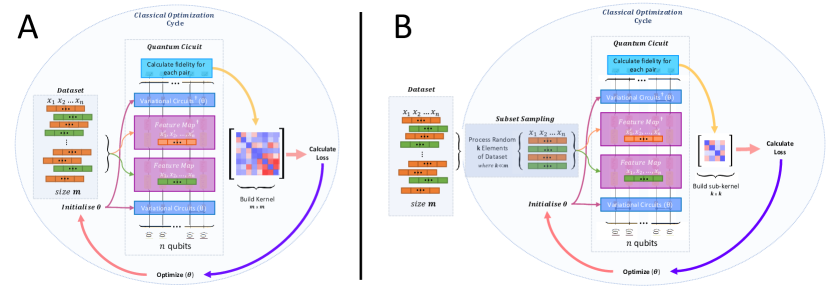
Figure 1: A) Quantum kernel alignment uses n qubits to encode the dataset into a feature map, estimate the kernel, and optimize parameters $\bm{\theta}$ until kernel separation improves. B) In the sub-sampling method, subsets with $k$ elements of the dataset are similarly processed using n qubits. This cycle repeats with different subsets, optimizing $\bm{\theta}$ until the entire dataset is sampled, yielding an optimized kernel. This will end with the estimation of the full dataset, optimised kernel.

II Methodology

Classical kernel methods compute elements of a kernel matrix $K_{x,x^{\prime}}$ using a kernel function $K(\bm{x},\bm{x}^{\prime})$ that measures the distance between two data points $\bm{x}$, $\bm{x}^{\prime}\in X$. For certain choices of distance measure it is possible to use the kernel trick to express the kernel function as an inner product in some vector space $V$. If the kernel function can be written as a feature map $f:X\rightarrow V$, then $V$ is known as the feature space and the kernel function can be written as an inner product on $V$, $K(\bm{x},\bm{x}^{\prime})=\langle f(\bm{x}),f(\bm{x}^{\prime})\rangle_{V}$. We can see from this definition that the kernel function is a measure of similarity between data points that takes on values $[0,1]$ e.g. if $x=x^{\prime}$ then the inner product is one, whereas if the maps $f(x)$, $f(x^{\prime})$ result in orthogonal vectors then the inner product is zero.

Quantum kernel methods can be defined analogously to classical kernel methods. A quantum feature map, $\phi(\bm{x})$, is used to transform classical data $\bm{x}$ into a corresponding quantum state $|\phi(\bm{x})\rangle$. The fidelity kernel between two classical data points, $\bm{x}$ and $\bm{x}^{\prime}$, is computed using the overlap of the related quantum states $K(\bm{x},\bm{x}^{\prime})=|\langle\psi(\bm{x})|\psi(\bm{x}^{\prime})\rangle|^{2}$, where $|\psi(\bm{x})\rangle=U_{\phi}(\bm{x})|0\rangle^{\otimes n}$ and $U_{\phi}(\bm{x})$ is the unitary that implements the quantum feature map. The quality of such kernels can be further improved by quantum kernel alignment techniques that parameterise the kernel and use a variational approach to optimize for the kernel for a specific dataset as suggested in Ref. Hubregtsen et al. [2022], Glick et al. [2021] (see Fig. 1). QKA adds a variational layer $U(\bm{\theta})$ to the kernel, where $\bm{\theta}$ are trainable parameters. The elements of the fidelity kernel matrix are computed in the same way, but now depend on $\bm{\theta}$ as shown in Equation 1,

$$K(\bm{x},\bm{x}^{\prime},\bm{\theta})=|\langle\psi(\bm{\theta},\bm{x})|\psi(\bm{\theta},\bm{x}^{\prime})\rangle|^{2},$$ (1)

where $|\psi(\bm{\theta},\bm{x})\rangle=U_{\phi}(\bm{x})U(\bm{\theta})|0\rangle^{\otimes n}$.

Similar to classical kernel alignment Cristianini et al. [2001], the training of the variational quantum kernel can be seen as finding a kernel that minimizes the upper bound of the SVM generalization error. This is equivalent to minimising a loss function $L$,

$$L(\bm{\theta},a)=\sum_{i}a_{i}-0.5\sum_{i,j}a_{i}a_{j}y_{i}y_{j}K(\bm{\theta},x_{i},x_{j}),$$ (2)

where $a_{i}$ and $a_{j}$ are the optimal Lagrange multipliers, and $y$ are the labels of the binary classification problem. The hinge loss, as a function of the variational kernel $K(\bm{\theta})$, is not generally convex, hence the loss landscape may include local minima, complicating the training process.

While kernel alignment has been shown to improve the performance of kernel methods, it comes at a cost: for every iteration of the training process, the full kernel must be constructed which for a dataset with $m$ points requires $m^{2}$ inner product evaluations. For quantum kernel alignment this translates to $m^{2}$ circuits per training iteration which, as the dataset grows, can become prohibitively costly. In this paper, we present a novel method that utilises a so-called sub-sampling approach to speed-up the model training process by reducing the number of circuits per training iteration.

The full kernel, $K_{f}(\bm{\theta})$ is defined on the full dataset $D$ whereas the sub-kernel $K_{s}(\bm{\theta})$ is defined using a subset of the data $D_{s}\subset D$ that is randomly sampled from $D$. The sub-kernel is used during the variational optimisation phase in order to find optimal parameters $\bm{\theta}_{opt}$. Once obtained, the parameters $\bm{\theta}_{opt}$ are used to construct the full fidelity kernel $K_{f}(\bm{\theta}_{opt})$, which is then used for SVC classification. The benefit of this approach is that fewer circuits are required to build a sub-kernel than the full kernel, therefore training using a sub-kernel can speed-up the training process by a (potentially large) constant factor. The method, schematically represented in Fig. 1 B, can be summarised as follows:

• Variational parameter initialisation: the variational parameters $\bm{\theta}$ of the quantum circuit are initialised as $\bm{\theta}_{init}$, giving an initial state $|\psi(\bm{\theta}_{init})\rangle$.

• Variational parameters and loss function optimisation loop: execute the optimisation loop and for each iteration, execute the following sub-steps:

  • Dataset subsampling: initiate by randomly selecting a distinct subset of $k$ data points from the full dataset and employ Equation (1) to construct a sub kernel, $K_{s}$. Note that each time a new subset is selected, it is composed of previously unselected points until the entire dataset is exhausted, at which point previously selected points may be used again.

  • Loss function estimation: compute the loss function $L$ using $K_{s}$ (Equation 2).

  • Loss function optimisation: perform an optimisation step on $L$ to update the parameters $\bm{\theta}$.

• Full kernel estimation: utilise the optimised parameters $\bm{\theta}_{opt}$ to compute the full quantum kernel $K_{f}(\bm{\theta}_{opt})$.

• Training of classifier: implement the full kernel in an SVC model for binary classification.

When introducing sub-sampling into the optimisation process, instead of computing the loss $L_{f}=L(D)$ over the full dataset $D$, the loss is evaluated on a sub-sample of size $k$, $L_{s}=L(D_{s})$. This introduces a sampling error $\epsilon_{s}$. Assuming the sub-samples are i.i.d., the expected sampling error can be bounded by $\mathbb{E}[|\epsilon_{s}|]\leq O\left(\frac{\sigma_{k}}{\sqrt{s}}\right)$, where $\sigma_{k}^{2}$ is the variance of the distribution of losses for a sub-sample of size $k$ and $s$ is the number of samples. In the limit that the sub-sample size is equal to the full dataset, then the variance in the loss goes to zero. We cannot say anything general about $\sigma_{k}$ as it will depend on the specifics of the dataset and the choice of $k$ among other things. However, we expect that sub-sampling will introduce some non-zero variance that could be large. The error in the loss can be controlled by taking multiple sub-samples and averaging them in each step of the training. Nonetheless, the variance in the loss will likely result in more training iterations being required to reach some fixed convergence criterion, compared to the full kernel training method.

In the case of training with a full kernel, every iteration involves processing all $m$ data points. The full kernel matrix contains $m^{2}$ entries which correspond to $m^{2}$ evaluations of the kernel function and therefore, assuming no noise, a query complexity of $O(m^{2})$ per training iteration. In the presence of finite sampling noise, it has been shown that sampling overhead results in a considerably worse complexity of $O(m^{4.67}/\epsilon^{2})$ per training iteration for a kernel that is $\epsilon$-close to the infinite shot kernel Gentinetta et al. [2022]. For the remainder of this work, we consider the noise-free case but note that the speed-ups presented may in fact improve in the presence of noise.

Denoting the number of iterations required for convergence as $T$, the overall complexity for the full kernel training is $O(m^{2}T)$. On the other hand, with sub-kernel training, we only process a subset of the data points of size $k$ at each iteration. Given $T^{\prime}$ training iterations and $s$ sub-kernels per iteration, the overall complexity of the sub-sampling approach is $O(sk^{2}T^{\prime})$. As discussed previously, it is likely that $T^{\prime}>T$ meaning it is not guaranteed that the complexity is reduced. It is evident that the upper bound on $T^{\prime}$ is given by $T^{\prime}<\frac{m^{2}}{sk^{2}}T$. Note that, while increasing $s$ decreases the upper bound on $T^{\prime}$, it also decreases the loss error $\epsilon_{s}$ in each iteration which in turn is likely to decrease the actual value of $T^{\prime}$. Assuming that $k<<m$ and that $s<m^{2}/k^{2}$, then $T^{\prime}$ is allowed to be a potentially large multiple of $T$. This opens up the possibility for considerable reductions in run time when training using the sub-sampling approach. While there are no a priori guarantees that $T^{\prime}$ will satisfy the bound given above, our results shown in the next section demonstrate significant speed-ups with little to no loss of classification accuracy relative to the full kernel method.

III Results from Numerical Simulations and Discussion

In this section we demonstrate our novel method by applying it to several test cases, showcasing the reductions in optimised kernel estimation times as well as retained - or improved - classification accuracy. We start by describing the setup of our tests and then we present results using two synthetic and one real-world dataset as examples.

Our experiments involved two variational ansatze: Real Amplitudes (RA) and Hardware Efficient (HE) Farhi et al. [2014], often referred to as Efficient SU2 ansatze. We used three different optimisers including Gradient Descent (GD) Bottou [2010], SPSA (Simultaneous Perturbation Stochastic Approximation) Spall [1998], ADAM (Adaptive Moment Estimation) Kingma and Ba [2014]. We employed multiple commonly used ansatze and optimisers to test whether or not these choices impact the performance of the sub-sample method. We used different feature maps to encode the data according to the dataset and specify each in the relevant sections. To ensure fairness and reproducibility, the same initial variational parameters are used for every run. Unless stated otherwise, the results presented were obtained from statevector simulations using Qiskit Aleksandrowicz et al. [2019]. The standard deviation of the outcomes through 10-fold cross-validation across all simulations was calculated. We maintained the same test and train subsets for all SVC methods to facilitate an accurate direct comparison between the different algorithms. All experiments were conducted five times, and the results shown are the averages over the values obtained.

In the results presented here, we use the number of queries as a figure of merit. This has the advantage of being a platform-independent metric. Here, a query refers to a single execution of a fidelity calculation i.e., a single circuit. By comparing the number of queries required to reach the optimal solution for each method, we can determine the relative speed-up one method has over another.

III.1 Synthetic Datasets

III.1.1 Benchmarking for Second-order Pauli-Z evolution circuit

For the empirical evaluation of our method, we use a synthetic dataset that is constructed in line with the principles set out by Havlíček et al. Havlíček et al. [2019], where the dataset is specifically designed to be fully separable through a second-order Pauli-Z evolution. The feature map transforms uniformly distributed vectors into quantum states, and labels are attributed based on the inner products of these quantum states. A separation gap of 0.2 is used to set the labeling threshold, ensuring a balanced yet challenging classification problem. The dataset comprises 96 training data points and 32 test data points, each represented by a 2-qubit quantum state.

In Table 1, we show the results obtained from statevector simulation using the SPSA optimiser with different ansatze, sub-samples sizes and the corresponding number of queries and relative speed-up compared to the full kernel evaluation. In this case, we set the maximum number of training iterations to 200 and if the optimiser reaches this point then we pick the point with the lowest loss. If the point with the lowest loss occurs before the final point, we consider this to be the stopping point of the run. All 3 optimisers tested performed comparably, for the full list of results, see the Tables in Appendix B.

Table 1: Results for SPSA optimizer, $k$ represents the sub-kernel sample size, and $s$ is the number of samples. The F1 and ROC scores are computed on the full, optimised kernel. Results are ordered by descending $k$ and grouped by ansatze.

Ansatz	k	s	ROC AUC	F1	Queries	Speed-up
HE	96	1	0.98	0.931	1.37 $\times 10^{6}$	1.00
HE	32	1	0.99	0.931	3.78 $\times 10^{5}$	3.64
HE	32	4	0.985	0.931	1.38 $\times 10^{6}$	1.01
HE	16	1	0.985	0.856	1.06 $\times 10^{5}$	13.03
HE	16	4	0.99	0.931	4.52 $\times 10^{5}$	3.05
HE	16	8	0.985	0.931	8.95 $\times 10^{5}$	1.54
RA	96	1	0.980	0.931	8.52 $\times 10^{5}$	1.00
RA	32	1	0.985	0.931	3.38 $\times 10^{4}$	25.25
RA	32	8	0.990	0.931	3.06 $\times 10^{6}$	0.28
RA	16	1	0.985	0.931	8.70 $\times 10^{4}$	9.79
RA	16	4	0.985	0.931	2.61 $\times 10^{5}$	3.26
RA	8	8	0.975	0.8986	2.27 $\times 10^{5}$	3.75

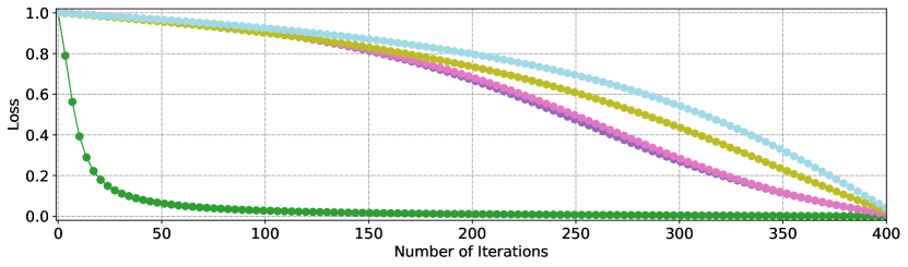
Figure 8: Min-Max normalised loss function for GD optimiser on COSETS problem.

The results demonstrate that the sub-sampling method can achieve similar performance using fewer circuits. The number of queries shown in Table 1 is the total number of queries, i.e. the number of queries per iteration multiplied by the number of iterations. We therefore see that, despite the sub-sampling method requiring more iterations to converge the loss function compared to the full kernel method (see Appendix C Figs 5 - 8), the total number of queries is still reduced considerably in almost all cases, resulting in up to x25 speed-up. The only case for which there is a slowdown is for the RA ansatz when $k=32$ and $s=8$. This is perhaps unsurprising given that $m=96$ and so with these parameters the ratio $m^{2}/sk^{2}$ is relatively close to 1. Furthermore, the accuracy of the classification is not deteriorated by the sub-sampling method, showing comparable or even improved accuracy compared to the calculation of the full kernel ($k=96$ and $s=1$ for both HE and RA ansatze).

We also performed a simple hardware experiment for this test case with the SPSA optimiser that can be seen in Appendix B Table 3. The experiments were performed on IBM Quantum hardware, Nairobi, using 2 qubits with 100 shots and no error mitigation. While we cannot draw general conclusions from these experiments, it is interesting to note that the speed-ups are realised even when measuring run time rather than queries. Furthermore, while the performance in terms of ROC AUC and F1 is lower in all cases (full and sub-kernel), we observe several cases where the sub-sampling method improves classification accuracy relative to the full kernel. This is some initial evidence that the method works on real hardware in the presence of noise.

III.1.2 Learning Problem Labeling Cosets with Error (LCE)

The second synthetic dataset we tested was the learning problem Labeling Cosets with Error (LCE) dataset, which was crafted to evaluate the accuracy of QML algorithms. The dataset was generated with a 27-qubit superconducting quantum processor Glick et al. [2021] which is split by 96 training points and 32 test points, each a 7-qubit quantum state defined by Euler angles. These angles specify elements of two separate cosets, forming the basis for binary classification. We apply the same feature map as used in Glick et al. [2021].

Table 2: Results for SPSA Optimizer on the Coset dataset, $k$ is the sub-kernel sample size, and $s$ is the number of samples. The F1 and ROC scores are computed on the full, optimised kernel. Results are ordered by descending $k$ and grouped by ansatze.

Ansatz	k	s	ROC AUC	F1	Queries	Speed-up
HE	96	1	1.00	1.00	1.40 x $10^{6}$	1.00
HE	32	1	1.00	1.00	3.83 x $10^{5}$	3.65
HE	32	4	1.00	1.00	1.54 x $10^{6}$	0.91
HE	16	1	1.00	1.00	1.13 x $10^{5}$	12.34
HE	16	4	1.00	1.00	4.55 x $10^{5}$	3.07
HE	16	8	1.00	0.97	9.01 x $10^{5}$	1.55
RA	96	1	1.00	1.00	1.43 x $10^{6}$	1.00
RA	32	1	1.00	1.00	3.86 x $10^{5}$	3.71
RA	32	4	1.00	1.00	1.51 x $10^{6}$	0.95
RA	16	1	1.00	1.00	1.06 x $10^{5}$	13.45
RA	16	4	1.00	1.00	4.46 x $10^{5}$	3.20
RA	16	8	1.00	0.96	9.17 x $10^{5}$	1.56

Similarly to Section 2.1.1, we present the results obtained using the SPSA optimiser in Table 2 (see Appendix D Tables for the full set of results). Also in this case, we observe over a $\times 10$ speed-up, with the number of queries reduced as we reduce $k$. The classification accuracy of the method is, once again, not affected by the method and agrees with our previous discussion in Section 2.1.1.

III.2 Real-World Dataset Experiment: Computational Pathology Breast Cancer Dataset

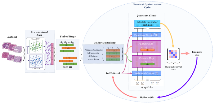
Figure 2: Combined GNN-extracted Pati et al. [2022] hierarchical cellular features with our sub-sampling method to optimise the creation of a quantum kernel used to classify subtypes of cancer. The AI-extracted embeddings are used to create the dataset that will be sampled using the methodology discussed in this work. The output of the workflow is a fully variationally optimised quantum kernel.

In the previous two subsections, we highlighted the strengths of our method with two synthetic datasets, showing that it’s possible to train a quantum kernel faster, and without compromising accuracy using a sub-sampling approach. To further substantiate these benefits, we tested our method on a real-world application where high classification accuracy is non-negotiable - computational pathology for detecting and subtyping cancer. We chose this as an example dataset because it is a classification problem that is known to be classically challenging and where small improvements in accuracy can have a significant real-world impact. While the aim of this work is not to improve accuracy over the state-of-the-art classical methods, we believe the speed-ups presented in this work may help to facilitate future progress towards this goal.

Accurate cancer detection and subtyping (i.e. the process of categorising a cancer into a more specific group based on its characteristics) O’Leary [2022], involves analyzing complex data from diagnostic images using Graph Neural Networks (GNNs). Typically the GNN is used to extract features that are then passed to a classifier Ahmedt-Aristizabal et al. [2022] (see Fig. 2). These classifiers have been shown to have high accuracy in classifying invasive vs non-invasive cancers but lower accuracy when classifying subtypes Pati et al. [2022].

In this work, we take the features extracted from a GNN using the framework as described in Pati et al. [2022] on breast cancer (BRACS) data. In the dataset, there are three distinct pathological benign lesions including Usual Ductal Hyperplasia (UDH), Flat Epithelial Atypia (FEA) and Atypical Ductal Hyperplasia (ADH), and malignant lesions including Ductal Carcinoma In Situ (DCIS) and Invasive Carcinoma (IC) besides Normal breast tissue. The subtypes are divided into two complex categories. The first category compares ADH and FEA to DCIS (1566 training points, 275 test points). In the second category Normal, and UDH are compared to ADH, FEA and DCIS (2797 Training points, 524 Test points).

In our tests, we used a 10-qubit feature map inspired by an instantaneous quantum polynomial (IQP) kernel Havlíček et al. [2019], Huang et al. [2021] with an optimal bandwidth parameter $c_{opt}\approx 2/n$ Shaydulin and Wild [2022], Canatar et al. [2022].

$$\begin{split}&U_{IQP}(x)=U_{Z}(x)\otimes H^{n}U_{Z}(x)\otimes H^{n},\\ &U_{Z}(x)=\exp\left(c\sum_{j=1}^{n}x_{j}Z_{j}+c^{2}\sum_{j,j^{\prime}=1}^{n}x_{j}x_{j^{\prime}}Z_{j}Z_{j^{\prime}}\right),\end{split}$$ (3)

where c is the bandwidth, $H$ and $Z$ denote the Hadamard and Pauli Z gates respectively.

It’s important to note that the results (shown in Fig. 3) are influenced by the inherent limitations of this feature map. Given that the goal of this work is to demonstrate the performance of the sub-sampling method, we chose this feature map not because it is optimal but simply because it is commonly used and readily available. We believe that it may be possible to improve classification accuracy beyond the results presented here by, for example, exploring different feature maps.

The results highlighted in Fig. 3 are collected to show the performance of the sub-sampling method comparing all the optimisers at once. In the same Figure, we also make the comparison between the classification accuracy of a GNN, classical kernels and a standard quantum fidelity kernel. In the case of the sub-kernel method applied to the real-world problem of cancer subtyping, we observe similar trends to those observed for the synthetic datasets discussed above. The sub-sampling method does not degrade the classification performance, and in some cases it improves the F1 score accuracy by a small amount (top panels in Fig. 3). It is also evident that the quantum kernel with QKA outperforms the standard quantum fidelity kernel in terms of classification accuracy (blue dotted line in Figure 3).

The advantages of employing the sub-sampling method to accelerate kernel training are also clear (bottom panels in Fig. 3). Given the substantial size of the full kernels in these cases (ranging from $\sim$1600 to $\sim$2800 data points), the reduction in queries is even more significant than previously observed, with some instances requiring three orders of magnitude fewer queries. When a kernel of size $m=2796$ is reduced to a sub-kernel of size $k=8$ and $s=1$, the number of queries is reduced by a factor of $1.6\times 10^{3}$. A table with the full results is available in Appendix D Tables 10 - XIII.

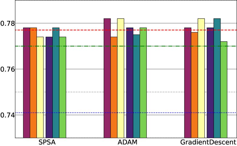
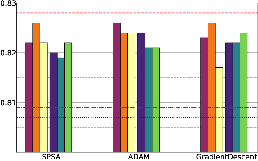
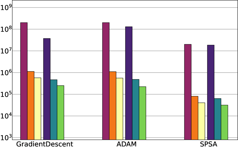
AF vs D

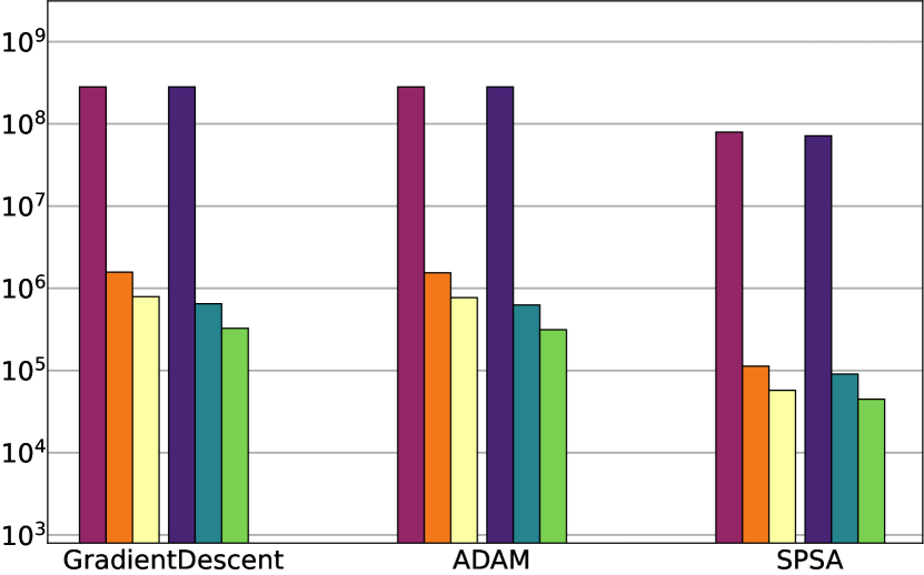
NBU vs AFD

Figure 3: Top left and right panels, F1 scores obtained with our method, grouped by optimiser (ADAM, GD and SPSA), using the full dataset and for the classification of AF vs D and NBU vs AFD cancer subtypes. Quantum fidelity kernel, best classical kernel and GNN reference values are represented as horizontal lines. Bottom left and right panels: total number of queries for each method, grouped by optimiser.

IV Conclusion

This study proposes a novel approach for implementing quantum kernel alignment for Support Vector Classification (SVC), introducing the use of sub-sampling during the quantum training phase. QKA is a method that is capable of improving the performance of quantum kernels. However, QKA comes at a significant cost due to the need to train the kernel. This cost has, until now, undermined the practical usefulness of quantum kernel alignment. However, our results have demonstrated that the sub-sampling method is a promising approach that makes QKA more viable in the near-term by considerably reducing number of circuits required to train the kernel. Importantly we have observed that this reduction in training cost does not necessarily come at the cost of classification accuracy.

While the sub-sampling method has the potential to speed-up the training process, there are no a priori guarantees that this will be the case. The actual reduction (or increase) in queries will depend on the choice of sub-kernel size, number of samples per training iteration and the specifics of the dataset. Nonetheless, in practice we have found that, in the cases tested, the speed-up is remarkably robust across different parameters, ansatzes and classical optimisers. The vast majority of instances tested resulted in reductions in number of circuits, even when testing on a real-world dataset. In fact the real-world dataset gave the best results with reductions of up to 3 orders of magnitude. Furthermore, the sub-sampling method introduces a level of stochastic optimisation which could lessen the severity of errors. This may explain why we observe improvements in classification accuracy in several cases when using the sub-sampling method. However, the stochastic nature of the training phase may also cause stability and reproducibility issues.

Appendix A Details of Experiments

In our numerical experiments, we utilized specific software and dataset settings to ensure reproducibility and precision. The software versions employed were Qiskit version 0.44, Qiskit Machine Learning version 0.6, and scikit-learn Version 1.3.0. For the Synthetic Benchmarking Dataset, the settings were: SPSA with 200 maximum iterations, a learning rate of 0.01, and a perturbation of 0.05; ADAM with 200 maximum iterations, a tolerance of 1e-06, and a learning rate of 0.01; Gradient Descent with 200 maximum iterations, a learning rate of 0.01, a tolerance of 1e-07, and no perturbation. For the COSET Dataset and the Computational Pathology Breast Cancer Dataset, maximum iterations were increased to 400 for all algorithms, keeping other parameters constant.

Using a validation set, which is split from the training set, a grid-search is performed over $C$ and $\gamma$ parameters as well as kernel type (Poly, RFB, Linear), and the best parameters and kernel type are then used to find best Classical Kernel to train the SVC algorithm. Similarly, a grid-search is performed over different $C$ values for the obtained quantum kernels using the same validation set.

Appendix B Results for Hardware run of Synthetic Dataset with SPSA Optimizer

The hardware used in this work is IBM Quantum Nairobi with Falcon r5.11H processor and 7 qubits. For qubit connectivity refer to Fig. 4. Qiskit options were set as initial_layout=[1,2], transpile=3 and resillience-level=0 with 100 shots.

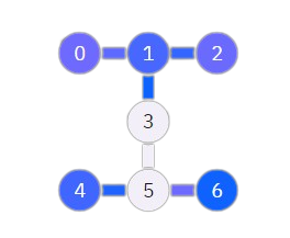
Figure 4: Schematic of the IBM Quantum Nairobi device taken at the time of the hardware experiments.

Table 3: Hardware results for SPSA Optimizer on the synthetic benchmarking dataset in section 2.1.1. $k$ is the sub-kernel sample size, and $s$ is the number of samples. The F1 and ROC scores are computed on the full, optimised kernel. Results are ordered by descending $k$ and grouped by ansatze. The runtime is calculated as the total hardware execution time inside an IBM Quantum Session.

Ansatz	k	s	ROC AUC	F1	Runtime (s)
HE	96	1	0.85	0.721	20155
HE	32	1	0.904	0.906	2819
HE	32	8	0.94	0.889	16331
HE	16	4	0.995	0.953	3590
HE	4	8	0.992	0.953	2422
RA	96	1	0.86	0.80	19453
RA	32	1	0.807	0.694	2864
RA	32	8	0.859	0.766	15506
RA	16	4	0.891	0.812	3851

Appendix C Loss Graphs

The magnitudes of the loss values computed for different settings can vary considerably due to the use of different kernel sizes, leading to significantly different scales of loss. Direct comparisons of these values are not informative because of this scale variation. To facilitate meaningful comparisons, min-max scaling is applied to each loss graph in Figs. 5 - 7, standardizing the range of values. The purpose of these plots is to demonstrate that, as expected, the sub-sampling method does result in the loss converging at a slower rate compared to the full kernel method.

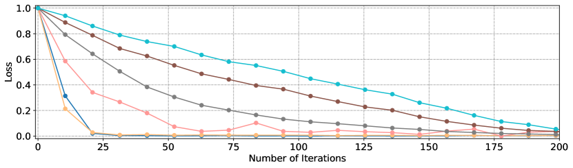
Figure 5: Min-Max normalised loss function for SPSA optimiser on the synthetic benchmarking dataset in section 2.1.1

Figure 6: Min-Max normalised loss function for GD optimiser on the synthetic benchmarking dataset in the section 2.1.1

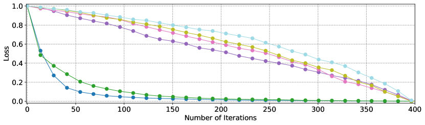
Figure 7: Min-Max normalised loss function for SPSA optimiser on COSETS problem.

Appendix D Numerical Results

Table 4: Results for SPSA Optimizer on the synthetic benchmarking dataset in section 2.1.1. $k$ is the sub-kernel sample size, and $s$ is the number of samples. The F1 and ROC scores are computed on the full, optimised kernel. Results are ordered by descending $k$ and grouped by ansatze.

Ansatz	k	s	ROC AUC	F1	Queries	Speed-up
HE	96	1	0.9800	0.9312	1377696.00	1.00
HE	32	1	0.9900	0.9312	378848.00	3.64
HE	32	4	0.9850	0.9312	1380320.00	1.00
HE	32	8	0.9800	0.9312	3125216.00	0.44
HE	16	1	0.9850	0.8561	105712.00	13.03
HE	16	4	0.9900	0.9312	452080.00	3.05
HE	16	8	0.9850	0.9312	894960.00	1.54
HE	8	1	0.9800	0.9312	14808.00	93.04
HE	8	4	0.9850	0.9312	108536.00	12.69
HE	8	8	0.9850	0.9312	213752.00	6.45
HE	4	1	0.9600	0.7407	3012.00	457.40
HE	4	4	0.9650	0.8667	26908.00	51.20
HE	4	8	1.0000	0.9312	54460.00	25.30
RA	96	1	0.9800	0.9312	852384.00	1.00
RA	32	1	0.9850	0.9312	33760.00	25.25
RA	32	4	0.9850	0.9312	1558496.00	0.55
RA	32	8	0.9900	0.9312	3063776.00	0.28
RA	16	1	0.9850	0.9312	87024.00	9.79
RA	16	4	0.9850	0.9312	260784.00	3.26
RA	16	8	0.8900	0.8244	919536.00	0.93
RA	8	1	0.9800	0.8624	27960.00	30.49
RA	8	4	0.9700	0.8986	101496.00	8.40
RA	8	8	0.9750	0.8986	227064.00	3.75
RA	4	1	0.9050	0.8244	4972.00	171.44
RA	4	4	0.9700	0.8986	28636.00	29.77
RA	4	8	0.8650	0.7634	56700.00	15.03

Table 5: Results for ADAM Optimizer on the synthetic benchmarking dataset in section 2.1.1. $k$ is the sub-kernel sample size, and $s$ is the number of samples. The F1 and ROC scores are computed on the full, optimised kernel. Results are ordered by descending $k$ and grouped by ansatze.

Ansatz	k	s	ROC AUC	F1	Queries	Speed-up
HE	96	1	0.9850	0.9312	6114720.00	1.00
HE	32	1	0.9700	0.7407	2157024.00	2.83
HE	32	4	0.9150	0.8244	3012576.00	2.03
HE	32	8	0.9600	0.8624	491488.00	12.44
HE	16	1	0.9500	0.8561	111472.00	54.85
HE	16	4	0.9550	0.8624	1893872.00	3.23
HE	16	8	0.9800	0.9312	902128.00	6.78
HE	8	1	0.9800	0.9312	344.00	17775.35
HE	8	4	0.9750	0.9662	689400.00	8.87
HE	8	8	0.9750	0.8624	158456.00	38.59
HE	4	1	0.9150	0.7937	60.00	101912.00
HE	4	4	0.9850	0.9312	148220.00	41.25
HE	4	8	0.9550	0.8624	344956.00	17.73
RA	96	1	0.9100	0.5333	350112.00	1.00
RA	32	1	0.9400	0.8986	56800.00	6.16
RA	32	4	0.9650	0.8244	88032.00	3.98
RA	32	8	0.9050	0.8000	9957344.00	0.04
RA	16	1	0.8700	0.6936	66416.00	5.27
RA	16	4	0.9850	0.8624	68080.00	5.14
RA	16	8	0.9750	0.8624	984048.00	0.36
RA	8	1	0.8500	0.8000	184.00	1902.78
RA	8	4	0.9150	0.8148	383736.00	0.91
RA	8	8	0.8700	0.7937	768248.00	0.46
RA	4	1	0.8950	0.8244	116.00	3018.21
RA	4	4	0.9700	0.9662	32060.00	10.92
RA	4	8	0.9300	0.8624	172732.00	2.03

Table 6: Results for GD Optimizer on the synthetic benchmarking dataset in section 2.1.1. $k$ is the sub-kernel sample size, and $s$ is the number of samples. The F1 and ROC scores are computed on the full, optimised kernel. Results are ordered by descending $k$ and grouped by ansatze.

Ansatz	k	s	ROC AUC	F1	Queries	Speed-up
HE	96	1	0.9800	0.9312	6437280.00	1.00
HE	32	1	0.9800	0.9312	1163232.00	5.53
HE	32	4	0.9850	0.9312	6948832.00	0.93
HE	32	8	0.9800	0.9312	13897696.00	0.46
HE	16	1	0.9800	0.9312	323952.00	19.87
HE	16	4	0.9900	0.8947	2047984.00	3.14
HE	16	8	0.9800	0.9312	4088816.00	1.57
HE	8	1	0.9700	0.8624	2520.00	2554.48
HE	8	4	0.9650	0.8947	511992.00	12.57
HE	8	8	0.9650	0.8986	1023224.00	6.29
HE	4	1	0.9750	0.8624	31876.00	201.95
HE	4	4	0.9750	0.8561	68668.00	93.74
HE	4	8	0.8500	0.7542	189180.00	34.03
RA	96	1	0.9800	0.9312	2386848.00	1.00
RA	32	1	0.9150	0.8310	1036768.00	2.30
RA	32	4	0.9850	0.9312	4171744.00	0.57
RA	32	8	0.8500	0.7333	8347616.00	0.29
RA	16	1	0.8650	0.5333	2416.00	987.93
RA	16	4	0.9850	0.9312	1226736.00	1.95
RA	16	8	0.9900	0.9312	2455536.00	0.97
RA	8	1	0.9450	0.8667	2520.00	947.16
RA	8	4	0.9300	0.8310	192376.00	12.41
RA	8	8	0.9700	0.8624	614392.00	3.88
RA	4	1	0.8100	0.7249	6244.00	382.26
RA	4	4	0.9850	0.8624	76604.00	31.16
RA	4	8	0.9150	0.7634	13564.00	175.97

Table 7: Results for SPSA Optimizer on the COSET dataset in section 2.1.2. $k$ is the sub-kernel sample size, and $s$ is the number of samples. The F1 and ROC scores are computed on the full, optimised kernel. Results are ordered by descending $k$ and grouped by ansatze.

Ansatz	k	s	ROC AUC	F1	Queries	Speed-up
HE	96	1	1.0000	1.0000	1396128.00	1.00
HE	32	1	1.0000	1.0000	382944.00	3.65
HE	32	4	1.0000	1.0000	1542112.00	0.91
HE	32	8	1.0000	1.0000	3125216.00	0.45
HE	16	1	1.0000	1.0000	113136.00	12.34
HE	16	4	1.0000	1.0000	455152.00	3.07
HE	16	8	1.0000	0.9687	901104.00	1.55
HE	8	1	0.9569	0.8110	11736.00	118.96
HE	8	4	0.8510	0.7500	96504.00	14.47
HE	8	8	0.7765	0.7500	228600.00	6.11
HE	4	1	0.7412	0.7500	1668.00	837.01
HE	4	4	0.7137	0.7500	18940.00	73.71
HE	4	8	0.6941	0.7179	35452.00	39.38
RA	96	1	1.0000	1.0000	1428384.00	1.00
RA	32	1	1.0000	1.0000	385504.00	3.71
RA	32	4	1.0000	1.0000	1507296.00	0.95
RA	32	8	1.0000	1.0000	3084256.00	0.46
RA	16	1	1.0000	1.0000	106224.00	13.45
RA	16	4	1.0000	1.0000	446448.00	3.20
RA	16	8	1.0000	0.9687	917488.00	1.56
RA	8	1	0.6157	0.6161	22040.00	64.81
RA	8	4	0.9255	0.8110	115064.00	12.41
RA	8	8	0.9137	0.8110	229880.00	6.21
RA	4	1	0.7882	0.7500	2972.00	480.61
RA	4	4	0.6980	0.7179	27516.00	51.91
RA	4	8	0.7686	0.7500	33660.00	42.44

Table 8: Results for ADAM Optimizer on the COSET dataset in section 2.1.2. $k$ is the sub-kernel sample size, and $s$ is the number of samples. The F1 and ROC scores are computed on the full, optimised kernel. Results are ordered by descending $k$ and grouped by ansatze.

Ansatz	k	s	ROC AUC	F1	Queries	Speed-up
HE	96	1	1.0000	1.0000	7741344.00	1.00
HE	32	1	0.9137	0.8110	2088928.00	3.71
HE	32	4	0.9765	0.8110	8173536.00	0.95
HE	32	8	0.9804	0.9375	5533664.00	1.40
HE	16	1	0.9176	0.8125	614512.00	12.60
HE	16	4	0.7176	0.7179	1090544.00	7.10
HE	16	8	0.8118	0.7500	4916208.00	1.57
HE	8	1	1.0000	1.0000	153272.00	50.51
HE	8	4	0.6941	0.7179	18936.00	408.82
HE	8	8	0.7255	0.7500	146424.00	52.87
HE	4	1	0.9843	0.9060	38268.00	202.29
HE	4	4	0.9725	0.8740	153500.00	50.43
HE	4	8	1.0000	1.0000	306812.00	25.23
RA	96	1	1.0000	1.0000	7741344.00	1.00
RA	32	1	0.7647	0.7500	1883616.00	4.11
RA	32	4	0.8980	0.8110	8355808.00	0.93
RA	32	8	0.8627	0.7806	16711648.00	0.46
RA	16	1	0.9961	0.8414	613872.00	12.61
RA	16	4	0.8118	0.7500	2391024.00	3.24
RA	16	8	0.7216	0.7500	3724272.00	2.08
RA	8	1	1.0000	1.0000	153528.00	50.42
RA	8	4	0.7373	0.7500	613496.00	12.62
RA	8	8	0.8275	0.7500	1229048.00	6.30
RA	4	1	1.0000	1.0000	38388.00	201.66
RA	4	4	1.0000	1.0000	153468.00	50.44
RA	4	8	0.7294	0.7500	137980.00	56.10

Table 9: Results for GD Optimizer on the COSET dataset in section 2.1.2. $k$ is the sub-kernel sample size, and $s$ is the number of samples. The F1 and ROC scores are computed on the full, optimised kernel. Results are ordered by descending $k$ and grouped by ansatze.

Ansatz	k	s	ROC AUC	F1	Queries	Speed-up
HE	96	1	1.0000	1.0000	5796768.00	1.00
HE	32	1	1.0000	1.0000	1564640.00	3.70
HE	32	4	1.0000	1.0000	6262752.00	0.93
HE	32	8	1.0000	1.0000	12525536.00	0.46
HE	16	1	1.0000	1.0000	403184.00	14.38
HE	16	4	1.0000	1.0000	1842160.00	3.15
HE	16	8	1.0000	1.0000	3684336.00	1.57
HE	8	1	0.4902	0.5795	4408.00	1315.06
HE	8	4	1.0000	1.0000	425976.00	13.61
HE	8	8	0.7451	0.6850	921080.00	6.29
HE	4	1	0.5804	0.5795	6036.00	960.37
HE	4	4	1.0000	0.9688	75004.00	77.29
HE	4	8	1.0000	1.0000	104700.00	55.37
RA	96	1	1.0000	1.0000	5796768.00	1.00
RA	32	1	1.0000	1.0000	774624.00	7.48
RA	32	4	1.0000	1.0000	6262752.00	0.93
RA	32	8	1.0000	1.0000	12525536.00	0.46
RA	16	1	0.9529	0.8750	311664.00	18.60
RA	16	4	1.0000	1.0000	1842160.00	3.15
RA	16	8	1.0000	1.0000	3684336.00	1.57
RA	8	1	0.7843	0.6161	28792.00	201.33
RA	8	4	0.9647	0.9060	118136.00	49.07
RA	8	8	0.7569	0.7500	921336.00	6.29
RA	4	1	1.0000	0.8740	22220.00	260.88
RA	4	4	1.0000	0.9060	107164.00	54.09
RA	4	8	0.7020	0.6161	198268.00	29.24

Table 10: Reference Values for AF vs D. The best Classical Kernel Represents the result of grid search as described in Appendix A. Classical NN Reference is the result from Pati et al. [2022]

	ROC	F1
Classical NN Reference	0.818	0.777
Best Classical Kernel	0.802	0.77
Quantum Fidelity Kernel	0.764	0.741

Table 11: Results for AF vs D dataset in section 2.1.3. Grouped by optimiser (ADAM, GD and SPSA) $k$ is the sub-kernel sample size, and $s$ is the number of samples. The F1 and ROC scores are computed on the full, optimised kernel. Results are ordered by descending $k$ and grouped by ansatze.

Optimizer	Ansatz	k	s	ROC AUC	F1	Queries	Speed-up
SPSA	HE	1566	1	0.793	0.778	2.01 x $10^{8}$	1.00
SPSA	HE	16	1	0.786	0.778	8.10 x $10^{5}$	248.02
SPSA	HE	16	4	0.793	0.778	0.81 x $10^{6}$	61.61
SPSA	HE	8	1	0.774	0.774	4.06 x $10^{5}$	494.25
SPSA	HE	8	4	0.788	0.781	0.41 x $10^{6}$	127.57
SPSA	RA	1566	1	0.745	0.774	1.85 x $10^{8}$	1.00
SPSA	RA	16	1	0.779	0.778	6.37 x $10^{5}$	291.11
SPSA	RA	16	4	0.789	0.763	0.64 x $10^{6}$	67.45
SPSA	RA	8	1	0.775	0.774	3.18 x $10^{5}$	583.09
SPSA	RA	8	4	0.773	0.763	0.32 x $10^{6}$	138.00
ADAM	HE	1566	1	0.791	0.782	2.02 x $10^{9}$	1.00
ADAM	HE	16	1	0.777	0.774	1.10 x $10^{7}$	182.47
ADAM	HE	16	4	0.787	0.774	1.10 x $10^{7}$	45.65
ADAM	HE	8	1	0.789	0.782	5.58 x $10^{6}$	361.05
ADAM	HE	8	4	0.784	0.767	0.56 x $10^{7}$	89.30
ADAM	RA	1566	1	0.774	0.778	1.30 x $10^{9}$	1.00
ADAM	RA	16	1	0.791	0.775	4.85 x $10^{6}$	268.40
ADAM	RA	16	4	0.775	0.774	0.48 x $10^{7}$	62.98
ADAM	RA	8	1	0.774	0.778	2.24 x $10^{6}$	580.27
ADAM	RA	8	4	0.770	0.762	2.24 x $10^{6}$	146.58
GD	HE	1566	1	0.775	0.778	2.02 x $10^{9}$	1.00
GD	HE	16	1	0.789	0.776	1.13 x $10^{7}$	178.41
GD	HE	16	4	0.782	0.782	1.13 x $10^{7}$	42.28
GD	HE	8	1	0.751	0.782	5.73 x $10^{6}$	351.83
GD	HE	8	4	0.775	0.782	0.57 x $10^{7}$	88.20
GD	RA	1566	1	0.783	0.778	3.75 x $10^{8}$	1.00
GD	RA	16	1	0.791	0.782	4.68 x $10^{6}$	80.06
GD	RA	16	4	0.783	0.770	0.47 x $10^{7}$	19.76
GD	RA	8	1	0.767	0.772	2.51 x $10^{6}$	149.21
GD	RA	8	4	0.795	0.778	2.51 x $10^{6}$	37.56

Table 12: Reference Values for NBU vs AFD. The best Classical Kernel Represents result of grid search as described in Appendix A. Classical NN Reference is the result from Pati et al. [2022]

	ROC	F1
Classical NN Reference	0.868	0.828
Best Classical Kernel	0.859	0.809
Quantum Fidelity Kernel	0.850	0.807

Table 13: Results for NBU vs AFD dataset in section 2.1.3. Grouped by optimiser (ADAM, GD and SPSA) $k$ is the sub-kernel sample size, and $s$ is the number of samples. The F1 and ROC scores are computed on the full, optimised kernel. Results are ordered by descending $k$ and grouped by ansatze.

Optimizer	Ansatz	k	s	ROC AUC	F1	Queries	Speed-up
SPSA	HE	2796	1	0.844	0.822	7.93 x $10^{8}$	1.00
SPSA	HE	16	1	0.834	0.826	1.13 x $10^{6}$	702.02
SPSA	HE	16	4	0.843	0.828	4.03 x $10^{6}$	174.29
SPSA	HE	8	1	0.833	0.822	5.74 x $10^{5}$	1382.46
SPSA	HE	8	4	0.836	0.828	0.57 x $10^{6}$	350.59
SPSA	RA	2796	1	0.830	0.820	7.14 x $10^{8}$	1.00
SPSA	RA	16	1	0.837	0.819	9.03 x $10^{5}$	790.26
SPSA	RA	16	4	0.833	0.820	0.90 x $10^{6}$	194.75
SPSA	RA	8	1	0.841	0.822	4.48 x $10^{5}$	1593.03
SPSA	RA	8	4	0.831	0.821	0.45 x $10^{6}$	370.98
ADAM	HE	2796	1	0.834	0.826	2.82 x $10^{9}$	1.00
ADAM	HE	16	1	0.833	0.824	1.54 x $10^{7}$	182.64
ADAM	HE	16	4	0.850	0.823	1.54 x $10^{7}$	43.07
ADAM	HE	8	1	0.826	0.824	7.71 x $10^{6}$	365.04
ADAM	HE	8	4	0.840	0.824	0.77 x $10^{7}$	93.90
ADAM	RA	2796	1	0.830	0.824	2.82 x $10^{9}$	1.00
ADAM	RA	16	1	0.841	0.821	6.27 x $10^{6}$	449.13
ADAM	RA	16	4	0.833	0.819	0.63 x $10^{7}$	111.20
ADAM	RA	8	1	0.848	0.821	3.14 x $10^{6}$	895.85
ADAM	RA	8	4	0.830	0.822	0.31 x $10^{7}$	224.12
GD	HE	2796	1	0.822	0.823	2.82 x $10^{9}$	1.00
GD	HE	16	1	0.836	0.826	1.58 x $10^{7}$	178.66
GD	HE	16	4	0.837	0.828	1.58 x $10^{7}$	42.07
GD	HE	8	1	0.835	0.828	7.92 x $10^{6}$	355.37
GD	HE	8	4	0.839	0.821	0.79 x $10^{7}$	90.22
GD	RA	2796	1	0.833	0.822	2.82 x $10^{9}$	1.00
GD	RA	16	1	0.840	0.822	6.49 x $10^{6}$	433.50
GD	RA	16	4	0.835	0.819	0.65 x $10^{7}$	111.94
GD	RA	8	1	0.843	0.824	3.26 x $10^{6}$	862.77
GD	RA	8	4	0.834	0.836	0.33 x $10^{7}$	207.59