Explicit numerical approximations for McKean-Vlasov stochastic differential equations in finite and infinite time

Abstract

By employing the stochastic particle method, this paper introduces the truncated Euler-Maruyama (TEM) method for the numerical solution of McKean-Vlasov stochastic differential equations (MV-SDEs), which may feature drift and diffusion coefficients with super-linear growth in the state variable. Initially, the propagation of chaos result is obtained in the $L^{q}$ sense under general assumptions. Subsequently, the proposed method s standard 1/2-order strong convergence rate in $L^{q}$ sense, corresponding to the particle system, is derived using the stopping time analysis techniques. Moreover, the TEM method allows for the numerical realization of long-time dynamical properties of MV-SDEs, such as moment boundedness, stability, and the existence and uniqueness of the invariant probability measure. Additionally, it is demonstrated that the numerical invariant measure converges to the underlying measure of MV-SDEs in the $L^{2}$-Wasserstein metric. Finally, the conclusions drawn in this paper are validated through examples and numerical simulations.

1 Introduction

MV-SDEs is a particular class of stochastic differential equations (SDEs) in which the drift and diffusion coefficients depend not only on the process state but also on the marginal laws of process. This is represented by the equation

$$\mathrm{d}X_{t}=f(X_{t},\mathcal{L}_{t}^{X})\mathrm{d}t+g(X_{t},\mathcal{L}_{t}^{X})\mathrm{d}B_{t},~{}~{}~{}\forall t\geq 0,$$ (1.1)

where $\mathcal{L}_{t}^{X}$ represents the distribution law of $X_{t}$. In terminology, MV-SDEs are also known as distribution-dependent SDEs or mean-field SDEs. McKean [30, 31] introduced MV-SDEs to model plasma dynamics. Since then, they have become an important tool for describing interacting systems with large numbers of particles and have been widely applied in various fields, including biological systems, financial engineering, and physics [2, 17, 6]. Various properties of MV-SDEs have been extensively investigated, such as well-posedness [37, 13, 18, 7, 34, 19], stability [11, 37, 1], and invariant measure [14, 37, 5, 38, 28], among others. In general, closed-form solutions of MV-SDEs are nearly impossible to obtain. Therefore, the objective of this paper is to develop a reliable numerical method for their simulations.

Solving MV-SDEs numerically presents an additional challenge compared to classical SDEs due to the need to discretize the distribution $\mathcal{L}^{X}_{t}$ in the equation coefficients. The stochastic particle method is commonly used for this purpose, which entails introducing a large interacting particle system (IPS) to approximate the original MV-SDEs. In this method, the true distribution $\mathcal{L}^{X}_{t}$ is approximated by the empirical distribution of particles, a concept known as propagation of chaos. To fully discretize the original MV-SDEs, it is essential to develop an effective numerical method for discretizing the IPS.

Currently, there have been some studies on the numerical approximation of McKean-Vlasov SDEs using the stochastic particle method. When the coefficients satisfy linear growth with respect to the state and measure, the Euler-Maruyama (EM) scheme has been employed for numerically simulating MV-SDEs [3, 10, 26]. However, numerous essential models exhibit superlinear growth, such as the stochastic mean-field FitzHugh-Nagumo model and the network of Hodgkin-Huxley neurons for neuron activation [2]. In 2011, Hutzenthaler et al. [20] highlighted that the $p$-th moments of the EM numerical solutions diverge to infinity for a class of SDEs with super-linear growth coefficients. This divergence is exacerbated in the particle systems corresponding to MV-SDEs due to the “particle corruption” effect [12]. Therefore, the EM scheme is ineffective for simulating MV-SDEs with super-linear growth coefficients.

Due to its simple algebraic structure and low computational cost, several modified EM methods have recently been developed for super-linear MV-SDEs. Inspired by [12], Dos Reis initially introduced the tamed EM scheme to simulate MV-SDEs with super-linear growth drift, achieving a convergence rate of $1/2$-order in time step size. Subsequently, the taming idea was applied to higher-order numerical schemes, resulting in the proposal of tamed Milstein schemes in [23, 4], which demonstrated strong convergence of order 1. Additionally, the tamed methods (including the tamed EM scheme and the tamed Milstein scheme) were extended to MV-SDEs with common noise, where the diffusion coefficient can grow super-linearly [24]. Moreover, the adaptive schemes, such as the adaptive Euler-Maruyama and the adaptive Milstein scheme, were also extended to MV-SDEs with a super-linear diffusion coefficient [33].

While explicit numerical methods have advantages in simulating super-linear MV-SDEs, modified EM methods still fall short in approximating the long-term dynamical properties of MV-SDEs. To date, there have been relatively few numerical approximation studies of the asymptotic properties of MV-SDEs. In 2003, Veretennikov [35] used the EM scheme to approximate the ergodic measure of MV-SDEs with additive noise and linearly bounded drift term. In 2022, Chen-Dos Reis [8] presented a sufficient condition for the mean-square contractivity of the implicit split-step Euler type method. Recently, Chen-Dos Reis-Stockinger [9] further utilized the implicit split-step Euler type method to demonstrate the mean-square contraction property of numerical solutions for a class of super-linear MV-SDEs, which possess drift and diffusion components of convolution type. To the best of our knowledge, there have been no published works addressing the numerical approximation of super-linear McKean-Vlasov processes in infinite time using explicit numerical methods. Therefore, we aim to construct proper explicit numerical methods for a class of MV-SDEs, allowing their numerical solutions to inherit the infinite-time dynamical properties of the exact solution.

About our research, we emphasize several key aspects: for classical SDEs, Li-Mao-Yin [27] developed various types of truncated EM (TEM) schemes with a $1/2$-order optimal rate and investigated the numerical approximations of the asymptotic properties by using the stopping time techniques. However, directly applying this technique to MV-SDEs is problematic because the solution of MV-SDE cannot be determined solely in a pathwise fashion [18, 26, 3, 29, 12]. Notably, our numerical scheme, based on the stochastic particle method, focuses on the corresponding IPS, which is a high-dimensional SDE. Therefore, our goal is to construct a proper TEM scheme that is applicable to the IPS corresponding to MV-SDE. Subsequently, by leveraging the result of the propagation of chaos, we anticipate achieving the numerical approximation of the asymptotic properties of the original MV-SDEs, including moment boundedness, exponential stability, and the existence and uniqueness of the invariant probability measure, among others.

In this study, we employ the stochastic particle method to develop a proper TEM scheme for the approximation of MV-SDEs across finite and infinite time horizons. To enhance the accuracy of numerical solutions, we adjust their values at the grid points prior to each iteration based on the growth rates of the drift and diffusion coefficients. This ensures that the numerical solutions inherit the properties of the exact solutions. In summary, the main contributions of this paper are as follows:

• Utilizing the theory developed in [15] regarding the convergence rate of the empirical measure of the i.i.d. random variable sequence, we establish the propagation of chaos in the $L^{q},~{}(q\geq 2)$ sense under relaxed conditions.

• Using the truncation idea, we construct an easily implementable explicit TEM scheme with $1/2$-order convergence rate, designed for the numerical solution of IPS corresponding to super-linear MV-SDE. Furthermore, the TEM numerical solution can effectively preserve the moment boundedness property of the exact solution in finite time.

• We demonstrate that the TEM numerical solution can keep the asymptotic properties of the exact solutions of MV-SDE, including the uniform moment boundedness in infinite time, exponential stability and the existence and uniqueness of invariant probability measure in $\mathcal{P}_{2}(\mathbb{R}^{d})$. Furthermore, we show that the numerical invariant probability measure converges to the underlying one of MV-SDE under the $L^{2}$-Wasserstein distance.

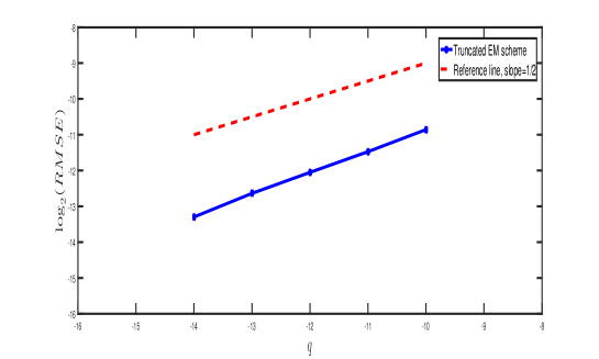
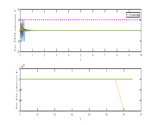
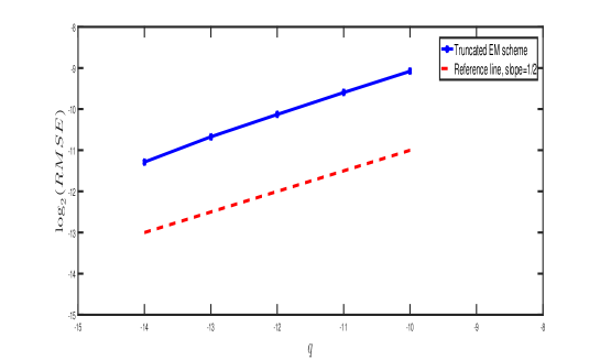
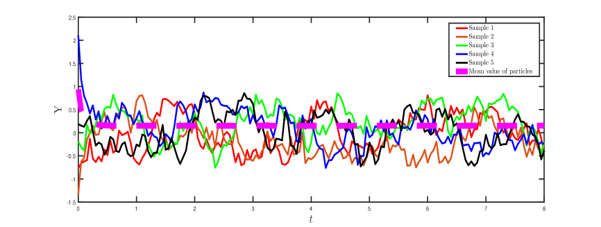
• We present a couple of numerical examples to support our theoretical findings.

The structure of this paper is as follows: In Section 2, we introduce some necessary notation and preliminary concepts. In Section 3, we establish the propagation of chaos result in the $L^{q},q\geq 2$ sense. Section 4 is dedicated to developing the truncated Euler-Maruyama (TEM) scheme for the IPS corresponding to MV-SDE, and we analyze its strong convergence within a finite time. Section 5 delves into the strong convergence rate of the TEM scheme. Section 6 investigates the asymptotic properties of the numerical solution obtained via the TEM scheme. Finally, Section 7 provides numerical examples to validate our theoretical findings.

2 Notations and preliminaries

Let $(\Omega,~{}\mathcal{F},~{}\mathbb{P},\{\mathcal{F}_{t}\}_{t\geq 0})$ be a complete probability space with a filtration $\{\mathcal{F}_{t}\}_{t\geq 0}$ satisfying the usual conditions (that is, it is right continuous and increasing while ${\mathcal{F}}_{0}$ contains all $\mathbb{P}$-null sets). $\{B_{t}\}_{t\geq 0}$ is a $m$-dimensional Brownian motion on probability space $(\Omega,~{}\mathcal{F},~{}\mathbb{P},\mathcal{F}_{t})$. Let $\mathbb{N}_{+}=\{1,2,\cdot\cdot\cdot\}$ be the set of positive integers. Use $|\cdot|$ to denote the Euclidean norm of $d$-dimensional vector and the trace norm of $d\times m$-matrix. For matrix $A\in\mathbb{R}^{d\times m}$, use $A^{T}$ to denote its transpose and its trace norm is $|A|=\sqrt{\mathrm{trace}(AA^{T})}$. For any $a,b\in\mathbb{R}$, let $a\wedge b=\min\{a,b\}$ and $a\vee b=\max\{a,b\}$. For a set $G$, let $I_{G}(x)=1$ if $x\in G$ and $0$ otherwise. Let $\mathcal{P}(\mathbb{R}^{d})$ denote the set of all the probability measures on the Euclidean space $\mathbb{R}^{d}$. If $\mu\in\mathcal{P}(\mathbb{R}^{d})$ and has a finite $q$-th moment, i.e.,

$$\mu(|\cdot|^{q}):=\int_{\mathbb{R}^{d}}|x|^{q}\mu(\mathrm{d}x)<\infty.$$ (2.1)

Then we define the subset of $\mathcal{P}(\mathbb{R}^{d})$ by

$$\mathcal{P}_{q}(\mathbb{R}^{d}):=\left\{\mu\in\mathcal{P}(\mathbb{R}^{d}):\mu(|\cdot|^{q})<\infty\right\}.$$

It is well known that $\mathcal{P}_{q}(\mathbb{R}^{d})$ is a polish space under the $L^{q}$-Wasserstein distance

$$\mathbb{W}_{q}(\mu,\nu)=\inf_{\pi\in\mathcal{C}(\mu,\nu)}\bigg{(}\int_{\mathbb{R}^{d}\times\mathbb{R}^{d}}|x-y|^{q}\pi(\mathrm{d}x,\mathrm{d}y)\bigg{)}^{\frac{1}{q}},$$

where $\mathcal{C}(\mu,\nu)$ is the set of all couplings for $\mu$ and $\nu$, namely, $\pi\in\mathcal{C}(\mu,\nu)$ if and only if $\pi(\cdot,\mathbb{R}^{d})=\mu(\cdot)$ and $\pi(\mathbb{R}^{d},\cdot)=\nu(\cdot)$. Especially, for any $\mu\in\mathcal{P}_{2}(\mathbb{R}^{d})$, $\mathbb{W}_{2}(\mu,\boldsymbol{\delta}_{0})=\mu^{\frac{1}{2}}(|\cdot|^{2})$ (see, [13, Lemma 2.3]), where $\boldsymbol{\delta}_{x}$ represents the Dirac measure concentrated at the point $x\in\mathbb{R}^{d}$. For $p\in[2,\infty)$, $L^{p}_{0}$ denote the family of $\mathbb{R}^{d}$-valued, $\mathcal{F}_{0}$-measurable random variables $\xi$, that satisfy $\mathbb{E}|\xi|^{p}<\infty$. For an $\mathbb{R}^{d}$-valued stochastic process $Z=\{Z_{t}\}_{t\geq 0}$, let $\mathcal{L}_{t}^{Z}$  denote the distribution law of $Z$ at time $t$. For convenience, use $C$ and $C_{l}$ to denote the generic positive constants whose value may change in different appearances, where $C_{l}$ is used to emphasize the dependence of $C$ on $l$. For clarity, we introduce some useful results. For $x:=(x_{1},\cdots,x_{M})\in\mathbb{R}^{dM}$, where $x_{i}\in\mathbb{R}^{d},1\leq i\leq M$, define

$$\mathcal{L}^{x,M}:=\frac{1}{M}\sum\limits_{i=1}^{M}\boldsymbol{\delta}_{x_{i}}\in\mathcal{P}(\mathbb{R}^{d}).$$

Recalling the definition (2.1), we know

$$\mathcal{L}^{x,M}(|\cdot|^{2})=\frac{1}{M}\sum_{i=1}^{M}|x_{i}|^{2}.$$ (2.2)

Obviously, for any $x=(x_{1},\cdots,x_{M})\in\mathbb{R}^{dM}$ and $y=(y_{1},\cdots,y_{M})\in\mathbb{R}^{dM}$,

$$\frac{1}{M}\sum\limits_{i=1}^{M}\big{(}\boldsymbol{\delta}_{x_{i}}\times\boldsymbol{\delta}_{y_{i}}\big{)}\in\mathcal{C}\Big{(}\mathcal{L}^{x,M},\mathcal{L}^{y,M}\Big{)}.$$

Thus,

$$\mathbb{W}^{2}_{2}\big{(}\mathcal{L}^{x,M},\mathcal{L}^{y,M}\big{)}\leq\frac{1}{M}\sum_{i=1}^{M}|x_{i}-y_{i}|^{2}.$$ (2.3)

This paper focuses on the MV-SDE (1.1) with initial value $X_{0}$, where

$$f:\mathbb{R}^{d}\times\mathcal{P}_{2}(\mathbb{R}^{d})\rightarrow\mathbb{R}^{d},~{}~{}~{}g:\mathbb{R}^{d}\times\mathcal{P}_{2}(\mathbb{R}^{d})\rightarrow\mathbb{R}^{d\times m}.$$

Next, we introduce several assumptions.

Assumption 1

There exists a pair of constants $p_{0}>2$ and $L_{1}>0$ such that

$$2(x_{1}-x_{2})^{T}\big{(}f(x_{1},\mu_{1})-f(x_{2},\mu_{2})\big{)}+(p_{0}-1)\left|g(x_{1},\mu_{1})-g(x_{2},\mu_{2})\right|^{2}\leq L_{1}\big{(}|x_{1}-x_{2}|^{2}+\mathbb{W}^{2}_{2}(\mu_{1},\mu_{2})\big{)}$$

for any $x_{1},x_{2}\in\mathbb{R}^{d}$ and $\mu_{1},\mu_{2}\in\mathcal{P}_{2}(\mathbb{R}^{d})$.

Assumption 2

There exists a pair of constants $p>2$ and $L_{2}>0$ such that

$$2x^{T}f(x,\mu)+(p-1)|g(x,\mu)|^{2}\leq L_{2}(1+|x|^{2}+\mu(|\cdot|^{2})).$$

for any $x\in\mathbb{R}^{d}$ and $\mu\in\mathcal{P}_{2}(\mathbb{R}^{d})$.

Assumption 3

For any $R>0$, there exists a constant $K_{R}>0$ such that

$$|f(x_{1},\mu)-f(x_{2},\mu)|\leq K_{R}|x_{1}-x_{2}|,$$ (2.4)

for any $x_{1},x_{2}\in\mathbb{R}^{d}$ with $|x_{1}|\vee|x_{2}|\leq R$ and $\mu\in\mathcal{P}_{2}(\mathbb{R}^{d})$. There exists a constant $K>0$ such that

$$|f(x,\mu_{1})-f(x,\mu_{2})|\leq K\mathbb{W}_{2}(\mu_{1},\mu_{2})$$ (2.5)

for any $x\in\mathbb{R}^{d}$ and $\mu_{1},\mu_{2}\in\mathcal{P}_{2}(\mathbb{R}^{d})$.

Remark 2.1

It is clear that Assumption 2 may be derived from Assumption 1 but with more complicated coefficient in front of $|g(x,\mu)|^{2}$. To keep the notation simple, we state Assumption 2 as a new assumption.

Remark 2.2

By Assumptions 1 and 3, we deduce that for any $R>0$, there is a constant $C_{R}>0$ such that for any $x_{1},x_{2}\in\mathbb{R}^{d}$ with $|x_{1}|\vee|x_{2}|\leq R$ and $\mu\in\mathcal{P}_{2}(\mathbb{R}^{d})$,

$$|g(x_{1},\mu)-g(x_{2},\mu)|^{2}\leq C_{R}|x_{1}-x_{2}|^{2}.$$ (2.6)

For any $x\in\mathbb{R}^{d}$ and $\mu_{1},\mu_{2}\in\mathcal{P}_{2}(\mathbb{R}^{d})$,

$$|g(x,\mu_{1})-g(x,\mu_{2})|^{2}\leq L_{2}\mathbb{W}^{2}_{2}(\mu_{1},\mu_{2}).$$ (2.7)

Lemma 2.3 ([24, Theorem 2.1])

Let Assumptions 1 and 2 hold and $X_{0}\in L^{p}_{0}$. Then MV-SDE (1.1) has a unique strong solution $X_{t}$ on $[0,\infty]$, which satisfies that

$$\sup_{t\in[0,T]}\mathbb{E}|X_{t}|^{p}\leq C_{T},~{}~{}~{}\forall T\geq 0.$$

3 Propagation of chaos

When constructing numerical schemes for MV-SDEs, a fundamental problem that we face is how to discretize the distribution law in coefficients. A common technique is to approximate the original MV-SDE by an interacting particle system [4, 33]. This approximation substitutes the marginal law in the MV-SDE coefficients with the empirical law of particles, known as the propagation of chaos [34, 25].

For any fixed $M\in\mathbb{N}_{+}$, let $\left(\{B^{i}_{t}\}_{t\geq 0},X^{i}_{0}\right),1\leq i\leq M$ be mutually independent copies of $\left(\{B_{t}\}_{t\geq 0},X_{0}\right)$ on the same probability space $(\Omega,\mathcal{F},\mathbb{P},\{\mathcal{F}_{t}\}_{t\geq 0})$. Then consider the interacting particle system (IPS) given by

$$\left\{\begin{array}[]{l}\mathrm{d}X^{i,M}_{t}=f\left(X^{i,M}_{t},\mathcal{L}_{t}^{X,M}\right)\mathrm{d}t+g\left(X^{i,M}_{t},\mathcal{L}_{t}^{X,M}\right)\mathrm{d}B^{i}_{t},~{}~{}~{}t\geq 0,\\ X^{i,M}_{t}|_{t=0}=X^{i}_{0},~{}~{}~{}1\leq i\leq M,\end{array}\right.$$ (3.1)

where

$$\mathcal{L}^{X,M}_{t}=\frac{1}{M}\sum_{i=1}^{M}\boldsymbol{\delta}_{X^{i,M}_{t}}$$

is the empirical distribution of particles $X^{i,M}_{t},~{}i=1,2,\cdot\cdot\cdot,M$. For the propagation of chaos result, we introduce the non-interacting particles system (NIPS) given by

$$\mathrm{d}X^{i}_{t}=f(X^{i}_{t},\mathcal{L}^{X^{i}}_{t})\mathrm{d}t+g(X^{i}_{t},\mathcal{L}^{X^{i}}_{t})\mathrm{d}B^{i}_{t},~{}~{}~{}\forall t\geq 0,$$ (3.2)

with the initial value $X^{i}_{0}$ for $1\leq i\leq M$. Due to the weak uniqueness established in Lemma 2.3, $\mathcal{L}^{X_{i}}_{t}=\mathcal{L}^{X}_{t},\forall t\geq 0$ for any $1\leq i\leq M$. Before proving the propagation of chaos, we cite an important result.

Lemma 3.1 ([15, Theorem 1])

Let $\left\{Z_{m}\right\}_{m\geq 1}$ be an i.i.d sequence of random variables on $\mathbb{R}^{d}$ with distribution $\mu\in\mathcal{P}_{\bar{q}}\left(\mathbb{R}^{d}\right)$. Define the empirical measure $\mu^{M}=\frac{1}{M}\sum_{j=1}^{M}\delta_{Z_{j}}$. Then for any $0<q<\bar{q}$, there exists a constant $C_{q,\bar{q},d}$ such that, for all $M\geq 1$,

$$\mathbb{E}\left[\mathbb{W}_{q}^{q}\left(\mu^{M},\mu\right)\right]\leq C_{q,\bar{q},d}\mu(|\cdot|^{\bar{q}})^{\frac{q}{\bar{q}}}\begin{cases}M^{-1/2}+M^{-(\bar{q}-q)/\bar{q}},&\text{ if }q>d/2\text{ and }\bar{q}\neq 2q,\\ M^{-1/2}\log(1+M)+M^{-(\bar{q}-q)/\bar{q}},&\text{ if }q=d/2\text{ and }\bar{q}\neq 2q,\\ M^{-q/d}+M^{-(\bar{q}-q)/\bar{q}},&\text{ if }2\leq q<d/2~{}\text{and}~{}\bar{q}\neq\frac{d}{d-q}.\end{cases}$$

Theorem 3.2 (Propagation of chaos)

Let Assumptions 1 and 2 hold. Then for any $X_{0}\in L^{p}_{0}$, $q\in[2,p)\wedge[2,p_{0}]$ and $T>0$, there exists a constant $C$ such that for any $T>0$,

$$\sup_{1\leq i\leq M}\sup_{0\leq t\leq T}\mathbb{E}\big{|}X^{i}_{t}-X^{i,M}_{t}\big{|}^{q}\leq C\Upsilon_{M,q,p,d},$$ (3.3)

and

$$\sup_{1\leq i\leq M}\sup_{0\leq t\leq T}\mathbb{E}\Big{[}\mathbb{W}^{q}_{2}\big{(}\mathcal{L}^{X^{i}}_{t},\mathcal{L}^{X,M}_{t}\big{)}\Big{]}\leq C\Upsilon_{M,q,p,d},$$ (3.4)

where

$$\Upsilon_{M,q,p,d}=\begin{cases}M^{-1/2}+M^{-(p-q)/p},&\text{ if }q>d/2\text{ and }p\neq 2q,\\ M^{-1/2}\log(1+M)+M^{-(p-q)/p},&\text{ if }q=d/2\text{ and }p\neq 2q,\\ M^{-q/d}+M^{-(p-q)/p},&\text{ if }2\leq q<d/2~{}\text{and}~{}p\neq\frac{d}{d-q},\end{cases}$$

and the constant $C$ is dependent on constants $q,p,d$ and $\sup\limits_{0\leq t\leq T}\mathbb{E}|X_{t}|^{p}$.

Proof. For convenience, define $\Xi^{i,M}_{t}=X^{i}_{t}-X^{i,M}_{t}$ for any $t\geq 0$. Using the Itô formula, we derive from (3.1) and (3.2) that for any $0\leq t\leq T$,

$$\mathrm{d}|\Xi^{i,M}_{t}|^{q} =\frac{q}{2}|\Xi^{i,M}_{t}|^{q-2}\Big{[}2(\Xi^{i,M}_{t})^{T}\left(f(X^{i}_{t},\mathcal{L}^{X^{i}}_{t})-f(X^{i,M}_{t},\mathcal{L}^{X,M}_{t})\right)\$$

$$~{}~{}~{}+(q-1)\left|g(X^{i}_{t},\mathcal{L}^{X^{i}}_{t})-g(X^{i,M}_{t},\mathcal{L}^{X,M}_{t})\right|^{2}\Big{]}\mathrm{d}t+\mathcal{M}^{i,M}_{t},$$

where

$$\mathcal{M}^{i,M}_{t}=q\int_{0}^{t}|\Xi^{i,M}_{s}|^{q-2}(\Xi^{i,M}_{s})^{T}\left(g(X^{i}_{s},\mathcal{L}^{X^{i}}_{s})-g(X^{i,M}_{s},\mathcal{L}^{X,M}_{s})\right)\mathrm{d}B^{i}_{s},$$

is a local martingale. Thus, thanks to $q\leq p_{0}$, by Assumption 1 we compute that

$$\mathbb{E}|\Xi^{i,M}_{t}|^{q} \leq\frac{qL_{2}}{2}\mathbb{E}\int_{0}^{t}|\Xi^{i,M}_{s}|^{q-2}\left(|\Xi^{i,M}_{s}|^{2}+\mathbb{W}_{2}^{2}(\mathcal{L}^{X^{i}}_{s},\mathcal{L}^{X,M}_{s})\right)\mathrm{d}s\$$

$$\leq C\int_{0}^{t}\mathbb{E}|\Xi^{i,M}_{s}|^{q}\mathrm{d}s+C\int_{0}^{t}\mathbb{E}\left[\mathbb{W}_{2}^{q}(\mathcal{L}^{X^{i}}_{s},\mathcal{L}^{X,M}_{s})\right]\mathrm{d}s.$$ (3.5)

For any $t\geq 0$, define

$$\mu^{M}_{t}:=\frac{1}{M}\sum_{i=1}^{M}\boldsymbol{\delta}_{X^{i}_{t}}.$$

Using the elementary inequality yields that for any $0\leq s\leq T$,

$$\mathbb{E}\left[\mathbb{W}^{q}_{2}(\mathcal{L}^{X^{i}}_{s},\mathcal{L}^{X,M}_{s})\right] \leq 2^{q-1}\Big{(}\mathbb{E}\left[\mathbb{W}^{q}_{2}(\mathcal{L}^{X^{i}}_{s},\mu^{M}_{s})\right]+\mathbb{E}\left[\mathbb{W}^{q}_{2}(\mu^{M}_{s},\mathcal{L}^{X,M}_{s})\right]\Big{)}.$$ (3.6)

Applying Lemma 3.1 with $\bar{q}=p$ yields that

$$\mathbb{E}\left[\mathbb{W}^{q}_{2}(\mathcal{L}^{X^{i}}_{s},\mu^{M}_{s})\right] \leq\mathbb{E}\left[\mathbb{W}^{q}_{q}(\mathcal{L}^{X^{i}}_{s},\mu^{M}_{s})\right]\leq C_{q,p,d}\mathbb{E}|X^{i}_{s}|^{\frac{q}{p}}\Upsilon_{M,q,p,d}\leq C_{q,p,d}\sup_{0\leq s\leq T}\mathbb{E}|X_{s}|^{\frac{q}{p}}\Upsilon_{M,q,p,d}.$$

On the other hand, since $\Xi^{i,M}_{s},i=1,\cdots,M$ are identically distributed, we have

$$\mathbb{E}\left[\mathbb{W}^{q}_{2}(\mu^{M}_{s},\mathcal{L}^{X,M}_{s})\right]\leq\frac{1}{M}\mathbb{E}|\Xi^{i,M}_{s}|^{q}=\mathbb{E}|\Xi^{i,M}_{s}|^{q},~{}~{}~{}\forall 1\leq i\leq M.$$

Inserting the above two inequalities into (3.6) and using Lemma 2.3 gives that

$$\mathbb{E}\left[\mathbb{W}^{q}_{2}(\mathcal{L}^{X^{i}}_{s},\mathcal{L}^{X,M}_{s})\right] \leq C\mathbb{E}|\Xi^{i,M}_{s}|^{q}+C_{q,p,d}\sup_{0\leq s\leq T}\mathbb{E}|X_{s}|^{\frac{q}{p}}\Upsilon_{M,q,p,d}\leq C\mathbb{E}|\Xi^{i,M}_{s}|^{q}+C\Upsilon_{M,q,p,d},$$ (3.7)

where the constant $C$ is dependent on $q,p,d$, and $\sup_{0\leq s\leq T}\mathbb{E}|X_{s}|^{\frac{q}{p}}$. Next, substituting the above inequality into (3) and then employing the Gronwall lemma we derive (3.3). Furthermore, inserting (3.3) into (3.7) implies (3.4) directly. The proof is complete.      

Lemma 3.3

Let Assumptions 1-2 hold. Then for any $X_{0}\in L^{p}_{0}$ and $T>0$,

$$\sup_{1\leq i\leq M}\sup_{0\leq t\leq T}\mathbb{E}|X^{i,M}_{t}|^{p}\leq C_{T}.$$

Furthermore, define the stopping time

$$\tau^{i,M}_{R}=\inf\left\{t\geq 0:|X^{i,M}_{t}|\geq R\right\}.$$ (3.8)

Then for any $T>0$,

$$\mathbb{P}\left(\tau^{i,M}_{R}\leq T\right)\leq\frac{C_{T}}{R^{p}}.$$

Proof. Using the Itô formula and Assumption 2 shows that for any $t\in[0,T]$ and $1\leq i\leq M$,

$$|X^{i,M}_{t}|^{p} \leq|X^{i}_{0}|^{p}+\frac{p}{2}\int_{0}^{t}|X^{i,M}_{s}|^{p-2}\left[2(X^{i,M}_{s})^{T}f(X^{i,M}_{s},\mathcal{L}^{X,M}_{s})+(p-1)\big{|}g(X^{i,M}_{s},\mathcal{L}^{X,M}_{s})\big{|}^{2}\right]\mathrm{d}s+\mathcal{M}^{i,M}_{t}\$$

$$\leq|X^{i}_{0}|^{p}+\frac{pL_{2}}{2}\int_{0}^{t}|X^{i,M}_{s}|^{p-2}\left(1+|X^{i,M}_{s}|^{2}+\mathcal{L}^{X,M}_{s}(|\cdot|^{2})\right)\mathrm{d}s+\mathcal{M}^{i,M}_{t},$$

where

$$\mathcal{M}^{i,M}_{t}=p\int_{0}^{t}|X^{i,M}_{s}|^{p-2}(X^{i,M}_{s})^{T}g(X^{i,M}_{s},\mathcal{L}^{X,M}_{s})\mathrm{d}B^{i}_{s}$$

is a local martingale. Employing the Young inequality and then taking expectation on both sides of the above inequality, we derive from (2.2) that

$$\mathbb{E}|X^{i,M}_{t}|^{p} \leq\mathbb{E}|X^{i}_{0}|^{p}+C\int_{0}^{t}\mathbb{E}\Big{[}1+|X^{i,M}_{s}|^{p}+\big{(}\mathcal{L}^{X,M}_{s}(|\cdot|^{2})\big{)}^{\frac{p}{2}}\Big{]}\mathrm{d}s\$$

$$\leq\mathbb{E}|X_{0}|^{p}+C\int_{0}^{t}\Big{[}1+\mathbb{E}|X^{i,M}_{s}|^{p}+\frac{1}{M}\sum_{i=1}^{M}\mathbb{E}|X^{i,M}_{s}|^{p}\Big{]}\mathrm{d}s.$$ (3.9)

Since $X^{i,M}_{s},i=1,\cdots,M$ are identically distributed for any $s\in[0,T]$, we further obtain that

$$\mathbb{E}|X^{i,M}_{t}|^{p}\leq\mathbb{E}|X_{0}|^{p}+C\int_{0}^{t}\big{(}1+\mathbb{E}|X^{i,M}_{s}|^{p}\big{)}\mathrm{d}s.$$ (3.10)

This, together with using the Gronwall inequality, implies that

$$\sup_{0\leq t\leq T}\mathbb{E}|X^{i,M}_{t}|^{p}\leq C_{T}.$$

Similar to derive (3) and (3.10), the above inequality is then used to obtain that

$$\mathbb{E}\Big{|}X^{i,M}_{T\wedge\tau^{i,M}_{R}}\Big{|}^{p} \leq\mathbb{E}|X_{0}|^{p}+C\mathbb{E}\int_{0}^{T\wedge\tau^{i,M}_{R}}\left[1+|X^{i,M}_{s}|^{p}+\big{(}\mathcal{L}^{X,M}_{s}(|\cdot|^{2})\big{)}^{\frac{p}{2}}\right]\mathrm{d}s\$$

$$\leq\mathbb{E}|X_{0}|^{p}+C\int_{0}^{T}\Big{(}1+\mathbb{E}|X^{i,M}_{s}|^{p}\Big{)}\mathrm{d}s\leq C_{T}.\$$

This implies that

$$R^{p}\mathbb{P}(\tau^{i,M}_{R}\leq T)\leq\mathbb{E}\Big{(}\big{|}X^{i,M}_{T\wedge\tau^{i,M}_{R}}\big{|}^{p}I_{\{\tau^{i,M}_{R}\leq T\}}\Big{)}\leq\mathbb{E}\big{|}X^{i,M}_{T\wedge\tau^{i,M}_{R}}\big{|}^{p}\leq C_{T},$$

and thus the second assertion follows directly. The proof is complete.      

4 TEM scheme and strong convergence

This section aims to construct an easily implementable numerical scheme for IPS (3.1) corresponding to MV-SDE (1.1) using the stochastic particle method and the truncation idea. Additionally, we will explore the strong convergence.

Initially, according to (2.4)-(2.7), we can choose a strictly increasing continuous function $\varphi:\mathbb{R}_{+}\rightarrow\mathbb{R}_{+}$, satisfying $\varphi(u)\rightarrow\infty$ as $u\rightarrow\infty$, such that

$$\sup_{\begin{subarray}{c}|x_{1}|\vee|x_{2}|\leq u\\ x_{1}\neq x_{2}\\ \mu_{1}\neq\mu_{2}\end{subarray}}\frac{|f(x_{1},\mu_{1})-f(x_{2},\mu_{2})|}{\big{(}|x_{1}-x_{2}|+\mathbb{W}_{2}(\mu_{1},\mu_{2})\big{)}}\vee\frac{|g(x_{1},\mu_{1})-g(x_{2},\mu_{2})|^{2}}{\big{(}|x_{1}-x_{2}|^{2}+\mathbb{W}^{2}_{2}(\mu_{1},\mu_{2})\big{)}}\leq\varphi(u).$$ (4.1)

Let $\varphi^{-1}$ denote the inverse function of $\varphi$. Note that $\varphi^{-1}:\mathbb{R}_{+}\rightarrow\mathbb{R}_{+}$ is also strictly increasing. Next we select a constant $K\geq|f(0,\boldsymbol{\delta}_{0})|\vee|g(0,\boldsymbol{\delta}_{0})|^{2}$, and further define a function $h(\Delta)=K\Delta^{-1/3}$ for $\Delta\in(0,1]$. Then for any given $\Delta\in(0,1]$, define the truncated mapping $\pi_{\Delta}:\mathbb{R}^{d}\rightarrow\mathbb{R}^{d}$ by

$$\pi_{\Delta}(x)=\Big{(}|x|\wedge\varphi^{-1}(h(\Delta))\Big{)}\frac{x}{|x|},~{}~{}~{}\forall x\in\mathbb{R}^{d},\$$

where the convention $x/|x|=\mathbf{0}\in\mathbb{R}^{d}$ when $x=\mathbf{0}$. Thus, one observes that for any $x,y\in\mathbb{R}^{d}$ and $\mu,\nu\in\mathcal{P}_{2}(\mathbb{R}^{d})$,

$$\big{|}f(\pi_{\Delta}(x),\mu)-f(\pi_{\Delta}(y),\nu)\big{|}\leq K\Delta^{-1/3}\big{(}|\pi_{\Delta}(x)-\pi_{\Delta}(y)|+\mathbb{W}_{2}(\mu,\nu)\big{)},$$ (4.2)

and

$$\big{|}g(\pi_{\Delta}(x),\mu)-g(\pi_{\Delta}(y),\nu)\big{|}^{2}\leq K\Delta^{-1/3}\big{(}|\pi_{\Delta}(x)-\pi_{\Delta}(y)|^{2}+\mathbb{W}^{2}_{2}(\mu,\nu)\big{)}.$$ (4.3)

Additionally, it is easy to deduce that for any $x\in\mathbb{R}^{d}$ and $\mu\in\mathcal{P}_{2}(\mathbb{R}^{d})$,

$$\big{|}f(\pi_{\Delta}(x),\mu)\big{|} \leq\big{|}f(\pi_{\Delta}(x),\mu)-f(0,\boldsymbol{\delta}_{0})\big{|}+\big{|}f(0,\boldsymbol{\delta}_{0})\big{|}\$$

$$\leq K\Delta^{-1/3}\big{(}|\pi_{\Delta}(x)|+\mathbb{W}_{2}(\mu,\boldsymbol{\delta}_{0})\big{)}+K\$$

$$\leq K\Delta^{-1/3}\big{(}1+|\pi_{\Delta}(x)|+\mu^{\frac{1}{2}}(|\cdot|^{2})\big{)},$$ (4.4)

and

$$\big{|}g(\pi_{\Delta}(x),\mu)\big{|}^{2}\leq 2K\Delta^{-1/3}\big{(}1+|\pi_{\Delta}(x)|^{2}+\mu(|\cdot|^{2})\big{)}.$$ (4.5)

Now we propose the TEM scheme: For any given $\Delta\in(0,1]$ and $t_{k}=k\Delta$,

$$\begin{cases}Y_{0}^{i,M}=\pi_{\Delta}(X_{0}^{i}),i=1,\cdots,M,\\ \mathcal{L}_{t_{k}}^{Y,M}=\frac{1}{M}\sum_{i=1}^{M}{\boldsymbol{\delta}_{Y_{t_{k}}^{i,M}}},\\ \bar{Y}_{t_{k+1}}^{i,M}=Y_{t_{k}}^{i,M}+f(Y_{t_{k}}^{i,M},\mathcal{L}_{t_{k}}^{Y,M})\Delta+g(Y_{t_{k}}^{i,M},\mathcal{L}_{t_{k}}^{Y,M})\Delta B_{t_{k}}^{i},\\ Y_{t_{k+1}}^{i,M}=\pi_{\Delta}(\bar{Y}_{t_{k+1}}^{i,M}),\\ \end{cases}$$ (4.6)

where $\Delta B^{i}_{t_{k}}=B^{i}_{t_{k+1}}-B^{i}_{t_{k}}$. Obviously, it follows from (4) and (4.5) that

$$\big{|}f(Y^{i,M}_{t_{k}},\mathcal{L}_{t_{k}}^{Y,M})\big{|}\leq K\Delta^{-1/3}\Big{[}1+|Y^{i,M}_{t_{k}}|+\big{(}\mathcal{L}_{t_{k}}^{Y,M}(|\cdot|^{2})\big{)}^{\frac{1}{2}}\Big{]},$$ (4.7)

and

$$\big{|}g(Y^{i,M}_{t_{k}},\mathcal{L}^{Y,M}_{t_{k}})\big{|}^{2}\leq 2K\Delta^{-1/3}\left(1+|Y^{i,M}_{t_{k}}|^{2}+\mathcal{L}^{Y,M}_{t_{k}}(|\cdot|^{2})\right).$$ (4.8)

Furthermore, define the piecewise contstant numerical solution by

$$Y^{i,M}_{t}:=Y^{i,M}_{t_{k}},~{}~{}~{}\forall~{}t\in[t_{k},t_{k+1}),~{}~{}1\leq i\leq M.$$

Lemma 4.1

Let Assumptions 1-3 hold. Then for any $X_{0}\in L^{p}_{0}$ and $T>0$,

$$\sup_{0<\Delta\leq 1}\sup_{0\leq t_{k}\leq T}\mathbb{E}\Big{(}\frac{1}{M}\sum_{i=1}^{M}|Y^{i,M}_{t_{k}}|^{2}\Big{)}^{\frac{p}{2}}\leq C_{T}.$$

Proof. From (4.6) we have

$$1+|\bar{Y}^{i,M}_{t_{k+1}}|^{2}=1+|Y^{i,M}_{t_{k}}|^{2}+\xi^{i,M}_{t_{k}},$$ (4.9)

where

$$\xi^{i,M}_{t_{k}} =2(Y^{i,M}_{t_{k}})^{T}f(Y^{i,M}_{t_{k}},\mathcal{L}^{Y,M}_{t_{k}})\Delta+\big{|}f(Y^{i,M}_{t_{k}},\mathcal{L}^{Y,M}_{t_{k}})\big{|}^{2}\Delta^{2}+\big{|}g(Y^{i,M}_{t_{k}},\mathcal{L}^{Y,M}_{t_{k}})\Delta B^{i}_{t_{k}}\big{|}^{2}\$$

$$~{}~{}~{}+2(Y^{i,M}_{t_{k}})^{T}g(Y^{i,M}_{t_{k}},\mathcal{L}^{Y,M}_{t_{k}})\Delta B^{i}_{t_{k}}+2f^{T}(Y^{i,M}_{t_{k}},\mathcal{L}^{Y,M}_{t_{k}})g(Y^{i,M}_{t_{k}},\mathcal{L}^{Y,M}_{t_{k}})\Delta B^{i}_{t_{k}}\Delta.$$ (4.10)

One observes that

$$1+\frac{1}{M}\sum_{i=1}^{M}|\bar{Y}^{i,M}_{t_{k+1}}|^{2}=1+\frac{1}{M}\sum_{i=1}^{M}|Y^{i,M}_{t_{k}}|^{2}+\frac{1}{M}\sum_{i=1}^{M}\xi^{i,M}_{t_{k}}.$$

Hence,

$$\Big{(}1+\frac{1}{M}\sum_{i=1}^{M}|\bar{Y}^{i,M}_{t_{k+1}}|^{2}\Big{)}^{\frac{p}{2}}=\Big{(}1+\frac{1}{M}\sum_{i=1}^{M}|Y^{i,M}_{t_{k}}|^{2}\Big{)}^{\frac{p}{2}}(1+\zeta_{t_{k}})^{\frac{p}{2}},$$ (4.11)

where

$$\zeta_{t_{k}}=\Big{(}1+\frac{1}{M}\sum_{i=1}^{M}|Y^{i,M}_{t_{k}}|^{2}\Big{)}^{-1}\Big{(}\frac{1}{M}\sum_{i=1}^{M}\xi^{i,M}_{t_{k}}\Big{)}.$$ (4.12)

Taking the conditional expectation on both sides of (4.11) yields that

$$\mathbb{E}\Big{[}\Big{(}1+\frac{1}{M}\sum_{i=1}^{M}|\bar{Y}^{i,M}_{t_{k+1}}|^{2}\Big{)}^{\frac{p}{2}}\Big{|}\mathcal{F}_{t_{k}}\Big{]}=\Big{(}1+\frac{1}{M}\sum_{i=1}^{M}|Y^{i,M}_{t_{k}}|^{2}\Big{)}^{\frac{p}{2}}\mathbb{E}\left[(1+\zeta_{t_{k}})^{\frac{p}{2}}|\mathcal{F}_{t_{k}}\right].$$ (4.13)

Recalling the Taylor expansion in [27], for $z>-1$, we obtain that

$$(1+z)^{\frac{p}{2}} \leq 1+\frac{p}{2}z+\frac{p(p-2)}{8}z^{2}+z^{3}P_{\iota}(z),~{}~{}\iota\in\mathbb{N}_{+},~{}2\iota<p\leq 2(\iota+1),$$ (4.14)

where $P_{\iota}(z)$ represents an $\iota$th-order polynomial of $z$ with coefficients dependent only on $p$. We are only proving the case $2<p\leq 4$ here and the other case can be handled similarly. According to (4.14), it follows that

$$\mathbb{E}\left[(1+\zeta_{t_{k}})^{\frac{p}{2}}|\mathcal{F}_{t_{k}}\right] \leq 1+\frac{p}{2}\mathbb{E}(\zeta_{t_{k}}|\mathcal{F}_{t_{k}})+\frac{p(p-2)}{8}\mathbb{E}\left(|\zeta_{t_{k}}|^{2}|\mathcal{F}_{t_{k}}\right)+\mathbb{E}\left(\zeta_{t_{k}}^{3}P_{\iota}(\zeta_{t_{k}})|\mathcal{F}_{t_{k}}\right).$$ (4.15)

Owing to the independence of  $\mathcal{F}_{t_{k}}$ and $\Delta B^{i}_{t_{k}}$ for $1\leq i\leq M$, we obtain that for any $A\in\mathbb{R}^{d\times m}$,

$$\mathbb{E}\left[(A\Delta B^{i}_{t_{k}})^{2\iota-1}|\mathcal{F}_{t_{k}}\right]=0,~{}~{}\forall\iota\in\mathbb{N}_{+},~{}~{}\mathbb{E}\left[|A\Delta B^{i}_{t_{k}}|^{2\gamma}|\mathcal{F}_{t_{k}}\right]=C\Delta^{\gamma},~{}~{}\forall\gamma>0.$$ (4.16)

This, together with (4.12), yields that

$$\mathbb{E}\big{(}\zeta_{t_{k}}|\mathcal{F}_{t_{k}}\big{)} =\Big{(}1+\frac{1}{M}\sum_{i=1}^{M}|Y^{i,M}_{t_{k}}|^{2}\Big{)}^{-1}\frac{1}{M}\sum_{i=1}^{M}\mathbb{E}\left(\xi^{i,M}_{t_{k}}|\mathcal{F}_{t_{k}}\right)\$$

$$\leq\Big{(}1+\frac{1}{M}\sum_{i=1}^{M}|Y^{i,M}_{t_{k}}|^{2}\Big{)}^{-1}\frac{1}{M}\sum_{i=1}^{M}\left[2(Y^{i,M}_{t_{k}})^{T}f(Y^{i,M}_{t_{k}},\mathcal{L}^{Y,M}_{t_{k}})+\big{|}g(Y^{i,M}_{t_{k}},\mathcal{L}^{Y,M}_{t_{k}})\big{|}^{2}\right]\Delta\$$

$$~{}~{}~{}+\Big{(}1+\frac{1}{M}\sum_{i=1}^{M}|Y^{i,M}_{t_{k}}|^{2}\Big{)}^{-1}\Big{[}\frac{1}{M}\sum_{i=1}^{M}\big{|}f(Y^{i,M}_{t_{k}},\mathcal{L}^{Y,M}_{t_{k}})\big{|}^{2}\Delta^{2}\Big{]}.$$

Furthermore, it follows from (2.2) and (4.7) that

$$\Big{(}1+\frac{1}{M}\sum_{i=1}^{M}|Y^{i,M}_{t_{k}}|^{2}\Big{)}^{-1}\Big{[}\frac{1}{M}\sum_{i=1}^{M}\big{|}f(Y^{i,M}_{t_{k}},\mathcal{L}^{Y,M}_{t_{k}})\big{|}^{2}\Delta^{2}\Big{]}\$$

$$\leq \Big{(}1+\frac{1}{M}\sum_{i=1}^{M}|Y^{i,M}_{t_{k}}|^{2}\Big{)}^{-1}\Big{[}\frac{1}{M}\sum_{i=1}^{M}3K^{2}\Delta^{\frac{4}{3}}\left(1+|Y^{i,M}_{t_{k}}|^{2}+\mathcal{L}^{Y,M}_{t_{k}}(|\cdot|^{2})\right)\Big{]}\$$

$$\leq \Big{(}1+\frac{1}{M}\sum_{i=1}^{M}|Y^{i,M}_{t_{k}}|^{2}\Big{)}^{-1}\Big{[}6K^{2}\Delta^{\frac{4}{3}}\Big{(}1+\frac{1}{M}\sum_{i=1}^{M}|Y^{i,M}_{t_{k}}|^{2}\Big{)}\Big{]}\leq C\Delta^{\frac{4}{3}}.\$$

As a result,

$$\mathbb{E}\big{(}\zeta_{t_{k}}|\mathcal{F}_{t_{k}}\big{)} \leq\Big{(}1+\frac{1}{M}\sum_{i=1}^{M}|Y^{i,M}_{t_{k}}|^{2}\Big{)}^{-1}\frac{1}{M}\sum_{i=1}^{M}\Big{[}2(Y^{i,M}_{t_{k}})^{T}f(Y^{i,M}_{t_{k}},\mathcal{L}^{Y,M}_{t_{k}})\$$

$$~{}~{}~{}+\big{|}g(Y^{i,M}_{t_{k}},\mathcal{L}^{Y,M}_{t_{k}})\big{|}^{2}\Big{]}\Delta+C\Delta^{\frac{4}{3}}.$$ (4.17)

For convenience, let $\xi^{i,M}_{t_{k}}=\sum_{l=1}^{5}Q^{i,M}_{t_{k},l}$, where

$$Q^{i,M}_{t_{k},1}=2(Y^{i,M}_{t_{k}})^{T}f(Y^{i,M}_{t_{k}},\mathcal{L}^{Y,M}_{t_{k}})\Delta,\$$

$$Q^{i,M}_{t_{k},2}=\big{|}f(Y^{i,M}_{t_{k}},\mathcal{L}^{Y,M}_{t_{k}})\big{|}^{2}\Delta^{2},\$$

$$Q^{i,M}_{t_{k},3}=\big{|}g(Y^{i,M}_{t_{k}},\mathcal{L}^{Y,M}_{t_{k}})\Delta B^{i}_{t_{k}}\big{|}^{2},\$$

$$Q^{i,M}_{t_{k},4}=2(Y^{i,M}_{t_{k}})^{T}g(Y^{i,M}_{t_{k}},\mathcal{L}^{Y,M}_{t_{k}})\Delta B^{i}_{t_{k}},\$$

$$Q^{i,M}_{t_{k},5}=2f^{T}(Y^{i,M}_{t_{k}},\mathcal{L}^{Y,M}_{t_{k}})g(Y^{i,M}_{t_{k}},\mathcal{L}^{Y,M}_{t_{k}})\Delta B^{i}_{t_{k}}\Delta.\$$

Performing a simple computation gives that

$$\mathbb{E}\big{(}|\zeta_{t_{k}}|^{2}|\mathcal{F}_{t_{k}}\big{)} =\Big{(}1+\frac{1}{M}\sum_{i=1}^{M}|Y^{i,M}_{t_{k}}|^{2}\Big{)}^{-2}\mathbb{E}\Big{[}\Big{(}\frac{1}{M}\sum_{i=1}^{M}\xi^{i,M}_{t_{k}}\Big{)}^{2}\Big{|}\mathcal{F}_{t_{k}}\Big{]}\$$

$$=\Big{(}1+\frac{1}{M}\sum_{i=1}^{M}|Y^{i,M}_{t_{k}}|^{2}\Big{)}^{-2}\frac{1}{M^{2}}\mathbb{E}\Big{[}\Big{(}\sum_{i=1}^{M}\xi^{i,M}_{t_{k}}\Big{)}^{2}\Big{|}\mathcal{F}_{t_{k}}\Big{]}\$$

$$\leq\Big{(}1+\frac{1}{M}\sum_{i=1}^{M}|Y^{i,M}_{t_{k}}|^{2}\Big{)}^{-2}\frac{1}{M^{2}}\mathbb{E}\Big{[}\Big{(}\sum_{l=1}^{5}\sum_{i=1}^{M}Q^{i,M}_{t_{k},l}\Big{)}^{2}\Big{|}\mathcal{F}_{t_{k}}\Big{]}\$$

$$\leq\Big{(}1+\frac{1}{M}\sum_{i=1}^{M}|Y^{i,M}_{t_{k}}|^{2}\Big{)}^{-2}\Big{(}\mathcal{A}_{1}+\mathcal{A}_{2}+\mathcal{A}_{3}\Big{)},$$ (4.18)

where

$$\mathcal{A}_{1}=4\sum_{1\leq l\leq 5,~{}l\neq 4}\frac{1}{M^{2}}\mathbb{E}\Big{[}\Big{(}\sum_{i=1}^{M}Q^{i,M}_{t_{k},l}\Big{)}^{2}\Big{|}\mathcal{F}_{t_{k}}\Big{]},$$

$$\mathcal{A}_{2}=\frac{1}{M^{2}}\mathbb{E}\Big{[}\Big{(}\sum_{i=1}^{M}Q^{i,M}_{t_{k},4}\Big{)}^{2}\Big{|}\mathcal{F}_{t_{k}}\Big{]},$$

and

$$\mathcal{A}_{3}=2\sum_{1\leq l\leq 5,l\neq 4}\frac{1}{M^{2}}\mathbb{E}\Big{[}\Big{(}\sum_{i=1}^{M}Q^{i,M}_{t_{k},l}\Big{)}\Big{(}\sum_{i=1}^{M}Q^{i,M}_{t_{k},4}\Big{)}\Big{|}\mathcal{F}_{t_{k}}\Big{]}.$$

Since the estimation of (4) is rather technical, we divide it into three steps.
Step 1: Estimate $\mathcal{A}_{1}$. Firstly, using (2.2), (4.16) and Assumption 2 yields that

$$\frac{1}{M^{2}}\mathbb{E}\Big{[}\Big{(}\sum_{i=1}^{M}Q^{i,M}_{t_{k},1}\Big{)}^{2}\Big{|}\mathcal{F}_{t_{k}}\Big{]} =\frac{1}{M^{2}}\Big{[}\sum_{i=1}^{M}2(Y^{i,M}_{t_{k}})^{T}f(Y^{i,M}_{t_{k}},\mathcal{L}^{Y,M}_{t_{k}})\Delta\Big{]}^{2}\$$

$$\leq\frac{1}{M^{2}}\Big{[}\sum_{i=1}^{M}C\Big{(}1+|Y^{i,M}_{t_{k}}|^{2}+\mathcal{L}^{Y,M}_{t_{k}}(|\cdot|^{2})\Big{)}\Big{]}^{2}\Delta^{2}\$$

$$\leq C^{2}\Delta^{2}\Big{[}\frac{1}{M}\sum_{i=1}^{M}\Big{(}1+|Y^{i,M}_{t_{k}}|^{2}+\mathcal{L}^{Y,M}_{t_{k}}(|\cdot|^{2})\Big{)}\Big{]}^{2}\$$

$$\leq C\Delta^{2}\Big{(}1+\frac{1}{M}\sum_{i=1}^{M}|Y^{i,M}_{t_{k}}|^{2}\Big{)}^{2}.$$ (4.19)

Likewise, utilizing (2.2), (4.7) and (4.16), we compute that

$$\frac{1}{M^{2}}\mathbb{E}\Big{[}\Big{(}\sum_{i=1}^{M}Q^{i,M}_{t_{k},2}\Big{)}^{2}\Big{|}\mathcal{F}_{t_{k}}\Big{]} =\frac{1}{M^{2}}\Big{(}\sum_{i=1}^{M}\big{|}f(Y^{i,M}_{t_{k}},\mathcal{L}^{Y,M}_{t_{k}})\big{|}^{2}\Delta^{2}\Big{)}^{2}\$$

$$\leq\frac{1}{M^{2}}\Big{[}\sum_{i=1}^{M}3K^{2}\Delta^{\frac{4}{3}}\Big{(}1+|Y^{i,M}_{t_{k}}|^{2}+\mathcal{L}^{Y.M}_{t_{k}}(|\cdot|^{2})\Big{)}\Big{]}^{2}\$$

$$\leq C\Delta^{\frac{8}{3}}\Big{(}1+\frac{1}{M}\sum_{i=1}^{M}|Y^{i,M}_{t_{k}}|^{2}\Big{)}^{2}.$$ (4.20)

Leveraging the mutual independence of $\Delta B^{i}_{t_{k}},i=1,\cdots,M$ implies that for any $1\leq i,j\leq M$,

$$\mathbb{E}\big{(}|\Delta B^{i}_{t_{k}}|^{\iota}|\Delta B^{j}_{t_{k}}|^{\gamma}|\mathcal{F}_{t_{k}}\big{)}=\Delta^{\frac{\iota+\gamma}{2}}.$$ (4.21)

This, along with (4.16), yields that

$$\frac{1}{M^{2}}\mathbb{E}\Big{[}\Big{(}\sum_{i=1}^{M}Q^{i,M}_{t_{k},3}\Big{)}^{2}\Big{|}\mathcal{F}_{t_{k}}\Big{]}\$$

$$= \frac{1}{M^{2}}\mathbb{E}\Big{[}\Big{(}\sum_{i=1}^{M}\big{|}g(Y^{i,M}_{t_{k}},\mathcal{L}^{Y,M}_{t_{k}})\Delta B^{i}_{t_{k}}\big{|}^{2}\Big{)}\Big{(}\sum_{j=1}^{M}\big{|}g(Y^{j,M}_{t_{k}},\mathcal{L}^{Y,M}_{t_{k}})\Delta B^{j}_{t_{k}}\big{|}^{2}\Big{)}\Big{|}\mathcal{F}_{t_{k}}\Big{]}\$$

$$= \frac{1}{M^{2}}\sum_{i=1}^{M}\sum_{j=1}^{M}\Big{[}\Big{(}\big{|}g(Y^{i,M}_{t_{k}},\mathcal{L}^{Y,M}_{t_{k}})\big{|}^{2}\big{|}g(Y^{j,M}_{t_{k}},\mathcal{L}^{Y,M}_{t_{k}})\big{|}^{2}\Big{)}\mathbb{E}\Big{(}|\Delta B^{i}_{t_{k}}|^{2}|\Delta B^{j}_{t_{k}}|^{2}|\mathcal{F}_{t_{k}}\Big{)}\Big{]}\$$

$$\leq \frac{1}{M^{2}}\Big{(}\sum_{i=1}^{M}\big{|}g(Y^{i,M}_{t_{k}},\mathcal{L}^{Y,M}_{t_{k}})\big{|}^{2}\Big{)}^{2}\Delta^{2}.$$ (4.22)

Applying (2.2) and (4.8), we further deduce that

$$\frac{1}{M^{2}}\mathbb{E}\Big{[}\Big{(}\sum_{i=1}^{M}Q^{i,M}_{t_{k},3}\Big{)}^{2}\Big{|}\mathcal{F}_{t_{k}}\Big{]} \leq\frac{1}{M^{2}}\Big{[}\sum_{i=1}^{M}2K\Delta^{-\frac{1}{3}}\Big{(}1+|Y^{i,M}_{t_{k}}|^{2}+\mathcal{L}^{Y,M}_{t_{k}}(|\cdot|^{2})\Big{)}\Big{]}^{2}\Delta^{2}\$$

$$\leq 4K^{2}\Delta^{\frac{4}{3}}\Big{[}\frac{1}{M}\sum_{i=1}^{M}\Big{(}1+|Y^{i,M}_{t_{k}}|^{2}+\mathcal{L}^{Y,M}_{t_{k}}(|\cdot|^{2})\Big{)}\Big{]}^{2}\$$

$$\leq C\Delta^{\frac{4}{3}}\Big{(}1+\frac{1}{M}\sum_{i=1}^{M}|Y^{i,M}_{t_{k}}|^{2}\Big{)}^{2}.$$ (4.23)

By using similar analysis techniques used above, we also can derive that

$$\frac{1}{M^{2}}\mathbb{E}\Big{[}\Big{(}\sum_{i=1}^{M}Q^{i,M}_{t_{k},5}\Big{)}^{2}\big{|}\mathcal{F}_{t_{k}}\Big{]} \leq\frac{4\Delta^{2}}{M^{2}}\mathbb{E}\Big{[}\Big{(}\sum_{i=1}^{M}\big{|}f(Y^{i,M}_{t_{k}},\mathcal{L}^{Y,M}_{t_{k}})\big{|}\big{|}g(Y^{i,M}_{t_{k}},\mathcal{L}^{Y,M}_{t_{k}})\big{|}\big{|}\Delta B^{i}_{t_{k}}\big{|}\Big{)}^{2}\Big{|}\mathcal{F}_{t_{k}}\Big{]}\$$

$$\leq\frac{4\Delta^{3}}{M^{2}}\Big{(}\sum_{i=1}^{M}\big{|}f(Y^{i,M}_{t_{k}},\mathcal{L}^{Y,M}_{t_{k}})\big{|}\big{|}g(Y^{i,M}_{t_{k}},\mathcal{L}^{Y,M}_{t_{k}})\big{|}\Big{)}^{2}\$$

$$\leq\frac{CK^{3}\Delta^{2}}{M^{2}}\Big{[}\sum_{i=1}^{M}\Big{(}1+|Y^{i,M}_{t_{k}}|^{2}+\mathcal{L}^{Y,M}_{t_{k}}(|\cdot|^{2})\Big{)}\Big{]}^{2}\$$

$$\leq C\Delta^{2}\Big{(}1+\frac{1}{M}\sum_{i=1}^{M}|Y^{i,M}_{t_{k}}|^{2}\Big{)}^{2}.$$

Combining (4), (4), (4) and the above inequality implies that

$$\mathcal{A}_{1}\leq C\Delta\Big{(}1+\frac{1}{M}\sum_{i=1}^{M}|Y^{i,M}_{t_{k}}|^{2}\Big{)}^{2}.$$ (4.24)

Step 2: Estimate $\mathcal{A}_{2}$. Similar to the proof of (4), we derive that

$$\mathcal{A}_{2} \leq\frac{1}{M^{2}}\mathbb{E}\Big{[}\Big{(}\sum_{i=1}^{M}2|Y^{i,M}_{t_{k}}|\big{|}g(Y^{i,M}_{t_{k}},\mathcal{L}^{Y,M}_{t_{k}})\big{|}|\Delta B^{i}_{t_{k}}|\Big{)}^{2}\Big{|}\mathcal{F}_{t_{k}}\Big{]}\$$

$$=\frac{1}{M^{2}}\Big{(}\sum_{i=1}^{M}2\big{|}Y^{i,M}_{t_{k}}\big{|}\big{|}g(Y^{i,M}_{t_{k}},\mathcal{L}^{Y,M}_{t_{k}})\big{|}\Big{)}^{2}\Delta.$$

By using the Cauchy-Schwarz inequality, it follows that

$$\mathcal{A}_{2} \leq\frac{1}{M^{2}}\Big{(}\sum_{i=1}^{M}|Y^{i,M}_{t_{k}}|^{2}\Big{)}\Big{(}\sum_{i=1}^{M}4\big{|}g(Y^{i,M}_{t_{k}},\mathcal{L}^{Y,M}_{t_{k}})\big{|}^{2}\Big{)}\Delta$$ (4.25)

$$=\Big{(}\frac{1}{M}\sum_{i=1}^{M}|Y^{i,M}_{t_{k}}|^{2}\Big{)}\Big{(}\frac{1}{M}\sum_{i=1}^{M}4\big{|}g(Y^{i,M}_{t_{k}},\mathcal{L}^{Y,M}_{t_{k}})\big{|}^{2}\Big{)}\Delta.$$

Step3: Estimate $\mathcal{A}_{3}$. In view of (4.16), we have that for any $1\leq i,j\leq M$,

$$\frac{1}{M^{2}}\mathbb{E}\Big{[}\Big{(}\sum_{i=1}^{M}Q^{i,M}_{1}\Big{)}\Big{(}\sum_{i=1}^{M}Q^{i,M}_{4}\Big{)}\Big{|}\mathcal{F}_{t_{k}}\Big{]}=\frac{1}{M^{2}}\sum_{i,j=1}^{M}\mathbb{E}\Big{(}Q^{i,M}_{1}Q^{j,M}_{4}|\mathcal{F}_{t_{k}}\Big{)}\$$

$$= \frac{4\Delta}{M^{2}}\sum_{i,j=1}^{M}\mathbb{E}\left[(Y^{i,M}_{t_{k}})^{T}f(Y^{i,M}_{t_{k}},\mathcal{L}^{Y,M}_{t_{k}}\big{)}\big{(}Y^{j,M}_{t_{k}}\big{)}^{T}g(Y^{j,M}_{t_{k}},\mathcal{L}^{Y,M}_{t_{k}}\big{)}\Delta B^{j}_{t_{k}}\big{|}\mathcal{F}_{t_{k}}\right]=0.$$ (4.26)

Similarly, we also obtain

$$\frac{1}{M^{2}}\mathbb{E}\Big{[}\Big{(}\sum_{i=1}^{M}Q^{i,M}_{2}\Big{)}\Big{(}\sum_{i=1}^{M}Q^{i,M}_{4}\Big{)}\Big{|}\mathcal{F}_{t_{k}}\Big{]}=0.$$ (4.27)

By (4.16), it is easy to prove that for any $1\leq i,j\leq M$,

$$\mathbb{E}\Big{(}|\Delta B^{i}_{t_{k}}|^{2}\Delta B^{j}_{t_{k}}|\mathcal{F}_{t_{k}}\Big{)}=0.$$

Using this we yield that

$$\frac{1}{M^{2}}\sum_{i,j=1}^{M}\mathbb{E}\Big{[}\Big{(}\sum_{i=1}^{M}Q^{i,M}_{3}\Big{)}\Big{(}\sum_{i=1}^{M}Q^{i,M}_{4}\Big{)}\Big{|}\mathcal{F}_{t_{k}}\Big{]}\$$

$$= \frac{1}{M^{2}}\sum_{i,j=1}^{M}2\big{|}g(Y^{i,M}_{t_{k}},\mathcal{L}^{Y,M}_{t_{k}})\big{|}^{2}(Y^{j,M}_{t_{k}})^{T}g(Y^{j,M}_{t_{k}},\mathcal{L}^{Y,M}_{t_{k}})\mathbb{E}\Big{(}|\Delta B^{i}_{t_{k}}|^{2}\Delta B^{j}_{t_{k}}|\mathcal{F}_{t_{k}}\Big{)}=0.$$ (4.28)

Utilizing (4.7), (4.8), and (4.21), and following a similar approach to proving (4), we infer that

$$\frac{1}{M^{2}}\mathbb{E}\Big{[}\Big{(}\sum_{i=1}^{M}Q^{i,M}_{5}\Big{)}\Big{(}\sum_{i=1}^{M}Q^{i,M}_{4}\Big{)}\big{|}\mathcal{F}_{t_{k}}\Big{]}\leq C\Delta^{\frac{4}{3}}\Big{(}1+\frac{1}{M}\sum_{i=1}^{M}|Y^{i,M}_{t_{k}}|^{2}\Big{)}^{2}.$$ (4.29)

Applying (4)-(4.29), we obtain that

$$\mathcal{A}_{3}\leq C\Delta^{\frac{4}{3}}\Big{(}1+\frac{1}{M}\sum_{i=1}^{M}|Y^{i,M}_{t_{k}}|^{2}\Big{)}^{2}.$$ (4.30)

Then substituting (4.24), (4.25) and (4.30) into (4) yields that

$$\mathbb{E}\big{(}|\zeta_{t_{k}}|^{2}|\mathcal{F}_{t_{k}}\big{)} \leq C\Delta^{\frac{4}{3}}+\Big{(}1+\frac{1}{M}\sum_{i=1}^{M}|Y^{i,M}_{t_{k}}|^{2}\Big{)}^{-1}\frac{1}{M}\sum_{i=1}^{M}4\big{|}g(Y^{i,M}_{t_{k}},\mathcal{L}^{Y,M}_{t_{k}})\big{|}^{2}\Delta.$$ (4.31)

Similarly, one also can show that for any $\iota\geq 3$,

$$\mathbb{E}\big{(}|\zeta_{t_{k}}|^{\iota}|\mathcal{F}_{t_{k}}\big{)}\leq C\Delta^{2}.$$ (4.32)

Subsequently, inserting (4), (4.31) and (4.32) into (4.15) shows that

$$\mathbb{E}\Big{[}(1+\zeta_{t_{k}})^{\frac{p}{2}}|\mathcal{F}_{t_{k}}\Big{]} \leq 1+C\Delta+\Big{(}1+\frac{1}{M}\sum_{i=1}^{M}|Y^{i,M}_{t_{k}}|^{2}\Big{)}^{-1}\times\frac{p}{2}\frac{1}{M}\sum_{i=1}^{M}\Big{[}2(Y^{i,M}_{t_{k}})^{T}f(Y^{i,M}_{t_{k}},\mathcal{L}^{Y,M}_{t_{k}})\$$

$$~{}~{}~{}+(p-1)\big{|}g(Y^{i,M}_{t_{k}},\mathcal{L}^{Y,M}_{t_{k}})\big{|}^{2}\Big{]}\Delta.$$

This, together with Assumption 2, implies that

$$\mathbb{E}\Big{[}(1+\zeta_{t_{k}})^{\frac{p}{2}}|\mathcal{F}_{t_{k}}\Big{]} \leq 1+C\Delta+\frac{pL_{1}\Delta}{2}\Big{(}1+\frac{1}{M}\sum_{i=1}^{M}|Y^{i,M}_{t_{k}}|^{2}\Big{)}^{-1}\frac{1}{M}\sum_{i=1}^{M}\Big{(}1+|Y^{i,M}_{t_{k}}|^{2}+\mathcal{L}^{Y,M}_{t_{k}}(|\cdot|^{2})\Big{)}\$$

$$\leq 1+C\Delta.$$

Plugging the above inequality into (4.13) yields that

$$\mathbb{E}\Big{[}\Big{(}1+\frac{1}{M}\sum_{i=1}^{M}|\bar{Y}^{i,M}_{t_{k+1}}|^{2}\Big{)}^{\frac{p}{2}}\Big{|}\mathcal{F}_{t_{k}}\Big{]}\leq(1+C\Delta)\Big{(}1+\frac{1}{M}\sum_{i=1}^{M}|Y^{i,M}_{t_{k}}|^{2}\Big{)}^{\frac{p}{2}}.$$

Thanks to the TEM scheme (4.6), taking expectation on both sides of the above inequality we derive that

$$\mathbb{E}\Big{(}1+\frac{1}{M}\sum_{i=1}^{M}|Y^{i,M}_{t_{k+1}}|^{2}\Big{)}^{\frac{p}{2}}\leq\mathbb{E}\Big{(}1+\frac{1}{M}\sum_{i=1}^{M}|\bar{Y}^{i,M}_{t_{k+1}}|^{2}\Big{)}^{\frac{p}{2}}\leq\big{(}1+C\Delta\big{)}\mathbb{E}\Big{(}1+\frac{1}{M}|Y^{i,M}_{t_{k}}|^{2}\Big{)}^{\frac{p}{2}}.$$

This iteration, together with the inequality $1+x\leq e^{x},~{}\forall 0\leq x$, leads to that

$$\mathbb{E}\Big{(}1+\frac{1}{M}\sum_{i=1}^{M}|Y^{i,M}_{t_{k}}|^{2}\Big{)}^{\frac{p}{2}} \leq(1+C\Delta)^{k}\mathbb{E}\Big{(}1+\frac{1}{M}\sum_{i=1}^{M}|Y^{i,M}_{0}|^{2}\Big{)}^{\frac{p}{2}}\$$

$$\leq C(1+\mathbb{E}|X^{i}_{0}|^{p})(1+C\Delta)^{k}\$$

$$=C(1+\mathbb{E}|X_{0}|^{p})(1+C\Delta)^{k}\leq Ce^{Ck\Delta}\leq Ce^{CT},$$

which implies the desired result.      

To analyze the moment boundedness, for any $1\leq i\leq M$, we further define an approximating process by

$$\tilde{Y}^{i,M}_{t} =Y^{i,M}_{t_{k}}+\int_{t_{k}}^{t}f(Y^{i,M}_{t_{k}},\mathcal{L}_{t_{k}}^{Y,M})\mathrm{d}t+\int_{t_{k}}^{t}g(Y^{i,M}_{t_{k}},\mathcal{L}_{t_{k}}^{Y,M})\mathrm{}\mathrm{d}B^{i}_{t},~{}~{}\forall t\in[t_{k},t_{k+1}),$$ (4.33)

Clearly, $\tilde{Y}^{i,M}_{t_{k}}=Y^{i,M}_{t_{k}}$, that is, $\tilde{Y}^{i,M}_{t}$ and $Y^{i,M}_{t}$ coincide at the grid points. In particular,

$$\lim_{t\rightarrow t^{-}_{k+1}}\tilde{Y}^{i,M}_{t}=\bar{Y}^{i,M}_{t_{k+1}}~{}~{}\mathrm{a.s.}$$ (4.34)

Lemma 4.2

Let Assumptions 1-3 hold. Then for any $X_{0}\in L^{p}_{0}$ and $T>0$,

$$\sup_{1\leq i\leq M}\sup_{0\leq\Delta\leq 1}\sup_{0\leq t_{k}\leq T}\mathbb{E}|Y^{i,M}_{t_{k}}|^{p}\leq C_{T}.$$

Proof. By the Itô formula, it follows from (4.33) and Assumption 2 that for any $t\in[t_{k},t_{k+1})$,

$$\mathbb{E}|\tilde{Y}^{i,M}_{t}|^{p} \leq\mathbb{E}|Y^{i,M}_{t_{k}}|^{p}+\frac{p}{2}\mathbb{E}\int_{t_{k}}^{t}|\tilde{Y}^{i,M}_{s}|^{p-2}\Big{[}2(\tilde{Y}^{i,M}_{s})^{T}f(Y^{i,M}_{t_{k}},\mathcal{L}^{Y,M}_{t_{k}})+(p-1)\big{|}g(Y^{i,M}_{t_{k}},\mathcal{L}^{Y,M}_{t_{k}})\big{|}^{2}\Big{]}\mathrm{d}s\$$

$$\leq\mathbb{E}|Y^{i,M}_{t_{k}}|^{p}+\frac{p}{2}\mathbb{E}\int_{t_{k}}^{t}|\tilde{Y}^{i,M}_{s}|^{p-2}\Big{[}2(Y^{i,M}_{t_{k}})^{T}f(Y^{i,M}_{t_{k}},\mathcal{L}^{Y,M}_{t_{k}})+(p-1)\big{|}g(Y^{i,M}_{t_{k}},\mathcal{L}^{Y,M}_{t_{k}})\big{|}^{2}\Big{]}\mathrm{d}s\$$

$$~{}~{}~{}+p\mathbb{E}\int_{t_{k}}^{t}|\tilde{Y}^{i,M}_{s}|^{p-2}|\tilde{Y}^{i,M}_{s}-Y^{i,M}_{t_{k}}|\big{|}f(Y^{i,M}_{t_{k}},\mathcal{L}^{Y,M}_{t_{k}})\big{|}\mathrm{d}s\$$

$$\leq\mathbb{E}|Y^{i,M}_{t_{k}}|^{p}+\frac{pL_{2}}{2}\mathbb{E}\int_{t_{k}}^{t}|\tilde{Y}^{i,M}_{s}|^{p-2}\big{(}1+|Y^{i,M}_{t_{k}}|^{2}+\mathcal{L}^{Y,M}_{t_{k}}(|\cdot|^{2})\big{)}\mathrm{d}s\$$

$$~{}~{}~{}+p\mathbb{E}\int_{t_{k}}^{t}|\tilde{Y}^{i,M}_{s}|^{p-2}|\tilde{Y}^{i,M}_{s}-Y^{i,M}_{t_{k}}|\big{|}f(Y^{i,M}_{t_{k}},\mathcal{L}^{Y,M}_{t_{k}})\big{|}\mathrm{d}s.\$$

Applying the Young inequality, (2.2) and Lemma 4.1, we derive that

$$\mathbb{E}|\tilde{Y}^{i,M}_{t}|^{p} \leq\mathbb{E}|Y^{i,M}_{t_{k}}|^{p}+C\int_{t_{k}}^{t}\mathbb{E}|\tilde{Y}^{i,M}_{s}|^{p}\mathrm{d}s+C\Delta\mathbb{E}|Y^{i,M}_{t_{k}}|^{p}+C\Delta\mathbb{E}\Big{(}\frac{1}{M}\sum_{i=1}^{M}\big{|}Y^{i,M}_{t_{k}}\big{|}^{2}\Big{)}^{\frac{p}{2}}\$$

$$~{}~{}~{}+C\int^{t}_{t_{k}}\mathbb{E}\Big{(}|\tilde{Y}^{i,M}_{s}-Y^{i,M}_{t_{k}}|^{\frac{p}{2}}\big{|}f(Y^{i,M}_{t_{k}},\mathcal{L}^{Y,M}_{t_{k}})\big{|}^{\frac{p}{2}}\Big{)}\mathrm{d}s+C\Delta\$$

$$\leq(1+C\Delta)\mathbb{E}|Y^{i,M}_{t_{k}}|^{p}+C\int_{t_{k}}^{t}\mathbb{E}|\tilde{Y}^{i,M}_{s}|^{p}\mathrm{d}s+C\Delta\$$

$$~{}~{}~{}+C\int^{t}_{t_{k}}\mathbb{E}\Big{(}|\tilde{Y}^{i,M}_{s}-Y^{i,M}_{t_{k}}|^{\frac{p}{2}}\big{|}f(Y^{i,M}_{t_{k}},\mathcal{L}^{Y,M}_{t_{k}})\big{|}^{\frac{p}{2}}\Big{)}\mathrm{d}s.$$ (4.35)

For any $s\in[0,T]$, there is a non-negative integer $k$ such that $s\in[t_{k},t_{k+1})$. Then applying (2.2), (4.7), (4.8) and Lemma 4.1 yields that

$$\mathbb{E}|\tilde{Y}^{i,M}_{s}-Y^{i,M}_{s}|^{p} =\mathbb{E}|\tilde{Y}^{i,M}_{s}-Y^{i,M}_{t_{k}}|^{p}\leq 2^{p-1}\left(\mathbb{E}\big{|}f(Y^{i,M}_{t_{k}},\mathcal{L}^{Y,M}_{t_{k}})\big{|}^{p}\Delta^{p}+\mathbb{E}\big{|}g(Y^{i,M}_{t_{k}},\mathcal{L}^{Y,M}_{t_{k}})\big{|}^{p}\Delta^{\frac{p}{2}}\right)\$$

$$\leq C\big{(}K^{p}\Delta^{\frac{2p}{3}}+K^{\frac{p}{2}}\Delta^{\frac{p}{3}}\big{)}\left[1+\mathbb{E}|Y^{i,M}_{t_{k}}|^{p}+\mathbb{E}\Big{(}\frac{1}{M}\sum_{i=1}^{M}|Y^{i,M}_{t_{k}}|^{2}\Big{)}^{\frac{p}{2}}\right]\$$

$$\leq C\Delta^{\frac{p}{3}}\big{(}1+\mathbb{E}|Y^{i,M}_{t_{k}}|^{p}\big{)}.$$ (4.36)

Using the elementary inequality, we obtain from (4) that for any $t_{k}\leq s<t_{k+1}$,

$$\mathbb{E}|\tilde{Y}^{i,M}_{s}|^{p} \leq 2^{p-1}\left(\mathbb{E}|\tilde{Y}^{i,M}_{s}-Y^{i,M}_{t_{k}}|^{p}+\mathbb{E}|Y^{i,M}_{t_{k}}|^{p}\right)\$$

$$\leq 2^{p-1}\left[C\Delta^{\frac{p}{3}}\big{(}1+\mathbb{E}|Y^{i,M}_{t_{k}}|^{p}\big{)}+\mathbb{E}|Y^{i,M}_{t_{k}}|^{p}\right]\$$

$$\leq C\big{(}1+\mathbb{E}|Y^{i,M}_{t_{k}}|^{p}\big{)}.$$ (4.37)

Moreover, by the Hölder inequality and the Young inequality, using (4.7), (4) and Lemma 4.1 leads to that for any $t_{k}\leq s<t_{k+1}$,

$$\mathbb{E}\Big{(}|\tilde{Y}^{i,M}_{s}-Y^{i,M}_{t_{k}}|^{\frac{p}{2}}\big{|}f(Y^{i,M}_{t_{k}},\mathcal{L}^{Y,M}_{t_{k}})\big{|}^{\frac{p}{2}}\Big{)}\leq\Big{(}\mathbb{E}|\tilde{Y}^{i,M}_{s}-Y^{i,M}_{t_{k}}|^{p}\Big{)}^{\frac{1}{2}}\Big{(}\mathbb{E}\big{|}f(Y^{i,M}_{t_{k}},\mathcal{L}^{Y,M}_{t_{k}})\big{|}^{p}\Big{)}^{\frac{1}{2}}\$$

$$\leq C\Delta^{\frac{p}{6}}K^{\frac{p}{2}}\Delta^{-\frac{p}{6}}\big{[}1+\big{(}\mathbb{E}|Y^{i,M}_{t_{k}}|^{p}\big{)}^{\frac{1}{2}}\big{]}\left\{1+\big{(}\mathbb{E}|Y^{i,M}_{t_{k}}|^{p}\big{)}^{\frac{1}{2}}+\Big{[}\mathbb{E}\Big{(}\frac{1}{M}\sum_{i=1}^{M}|Y^{i,M}_{t_{k}}|^{2}\Big{)}^{\frac{p}{2}}\Big{]}^{\frac{1}{2}}\right\}\$$

$$\leq C\big{[}1+\big{(}\mathbb{E}|Y^{i,M}_{t_{k}}|^{p}\big{)}^{\frac{1}{2}}\big{]}^{2}\leq C\big{(}1+\mathbb{E}|Y^{i,M}_{t_{k}}|^{p}\big{)}.$$ (4.38)

Then inserting (4) and (4) into (4) yields that

$$\mathbb{E}|\tilde{Y}^{i,M}_{t}|^{p} \leq(1+C\Delta)\mathbb{E}|Y^{i,M}_{t_{k}}|^{p}+C\Delta\big{(}1+\mathbb{E}|Y^{i,M}_{t_{k}}|^{p}\big{)},$$

which implies that

$$1+\mathbb{E}|\tilde{Y}^{i,M}_{t}|^{p}\leq(1+C\Delta)\left(1+\mathbb{E}|Y^{i,M}_{t_{k}}|^{p}\right).\$$

By virtue of the Fatou Lemma, we derive from (4.34) that

$$1+\mathbb{E}|Y^{i,M}_{t_{k+1}}|^{p}\leq 1+\mathbb{E}|\bar{Y}^{i,M}_{t_{k+1}}|^{p}=1+\lim_{t\rightarrow t^{-}_{k+1}}\mathbb{E}|\tilde{Y}^{i,M}_{t}|^{p}\leq(1+C\Delta)\left(1+\mathbb{E}|Y^{i,M}_{t_{k}}|^{p}\right).$$

This, together with the inequality $1+x\leq e^{x},0\leq x$, leads to that

$$\mathbb{E}|Y^{i,M}_{t_{k}}|^{p} \leq(1+C\Delta)(1+\mathbb{E}|Y^{i,M}_{t_{k-1}}|^{p})\cdots\leq e^{Ck\Delta}\big{(}1+\mathbb{E}|Y^{i,M}_{0}|^{p}\big{)}\$$

$$\leq e^{Ck\Delta}(1+\mathbb{E}|X^{i}_{0}|^{p})\leq e^{CT}\big{(}1+\mathbb{E}|X_{0}|^{p}\big{)}\leq C,$$

which implies the desired result.      

Corollary 4.3

Under the setting of Lemma 4.2, for any $T>0$,

$$\sup_{\Delta\in(0,1]}\sup_{1\leq i\leq M}\sup_{t\in[0,T]}\mathbb{E}|\tilde{Y}^{i,M}_{t}-Y^{i,M}_{t}|^{p}=C_{T}\Delta^{\frac{p}{3}}.$$

Proof. Combining Lemma 4.2 and (4) yields the desired result.      

Lemma 4.4

Let Assumptions 1-3 hold. Then for any $X_{0}\in L^{p}_{0}$ and $T>0$,

$$\sup_{1\leq i\leq M}\sup_{0<\Delta\leq 1}\sup_{0\leq t\leq T}\mathbb{E}|\tilde{Y}^{i,M}_{t}|^{p}\leq C_{T},$$

and

$$\sup_{1\leq i\leq M}\sup_{0<\Delta\leq 1}\sup_{0\leq t\leq T}\mathbb{E}\Big{(}|\tilde{Y}^{i,M}_{t}-Y^{i,M}_{t}|^{\frac{p}{2}}\big{|}f(Y^{i,M}_{t},\mathcal{L}^{Y,M}_{t})\big{|}^{\frac{p}{2}}\Big{)}\leq C_{T}.$$

Proof. For any $t\in[0,T]$, there is a non-negative integer $k$ such that $t\in[t_{k},t_{k+1})$. Then making use of Corollary 4.3 and Lemma 4.2, we derive that

$$\mathbb{E}|\tilde{Y}^{i,M}_{t}|^{p} \leq 2^{p-1}\Big{(}\mathbb{E}|\tilde{Y}^{i,M}_{t}-Y^{i,M}_{t_{k}}|^{p}+\mathbb{E}|Y^{i,M}_{t_{k}}|^{p}\Big{)}\$$

$$\leq 2^{p-1}\Big{[}C_{T}\Delta^{\frac{p}{3}}+\mathbb{E}|Y^{i,M}_{t_{k}}|^{p}\Big{]}\leq C_{T},$$

which implies the first desired result. Furthermore, it follows from (4) and Lemma 4.2 that

$$\mathbb{E}\Big{(}|\tilde{Y}^{i,M}_{t}-Y^{i,M}_{t}|^{\frac{p}{2}}|f(Y^{i,M}_{t},\mathcal{L}^{Y,M}_{t})|^{\frac{p}{2}}\Big{)} =\mathbb{E}\Big{(}|\tilde{Y}^{i,M}_{t}-Y^{i,M}_{t_{k}}|^{\frac{p}{2}}\big{|}f(Y^{i,M}_{t_{k}},\mathcal{L}^{Y,M}_{t_{k}})\big{|}^{\frac{p}{2}}\Big{)}\$$

$$\leq C\big{(}1+\mathbb{E}|Y^{i,M}_{t_{k}}|^{p}\big{)}\leq C_{T},$$

which suggests the second desired result. The proof is complete.      

Lemma 4.5

Assume that Assumptions 1-3 hold. For any $\Delta,\Delta_{1}\in(0,1]$, define the stopping time

$$\eta^{i,M}_{\Delta,\Delta_{1}}=\inf\left\{t\geq 0:|\tilde{Y}^{i,M}_{t}|\geq\varphi^{-1}(h(\Delta_{1}))\right\}.$$ (4.39)

Then for any $X_{0}\in L^{p}_{0}$ and $T>0$,

$$\mathbb{P}\left(\eta^{i,M}_{\Delta,\Delta_{1}}\leq T\right)\leq\frac{C_{T}}{\left[\varphi^{-1}(h(\Delta_{1}))\right]^{p}}.$$

Proof. The increasing of $\varphi^{-1}$ implies that $\varphi^{-1}(h(\Delta))\geq\varphi^{-1}(h(\Delta_{1}))$ for any $\Delta\in(0,\Delta_{1}]$. Thus, for any $0\leq t\leq T\wedge\eta^{i,M}_{\Delta,\Delta_{1}}$,

$$\tilde{Y}^{i,M}_{t}=Y^{i,M}_{0}+\int_{0}^{t}f(Y^{i,M}_{s},\mathcal{L}^{Y,M}_{s})\mathrm{d}s+\int_{0}^{t}g(Y^{i,M}_{s},\mathcal{L}^{Y,M}_{s})\mathrm{d}B^{i}_{s},$$

where

$$\mathcal{L}^{Y,M}_{s}=\frac{1}{M}\sum_{i=1}^{M}\boldsymbol{\delta}_{Y^{i,M}_{s}}.$$

Using techniques in the proofs of Lemma 3.3, we obtain the following inequality directly

$$\mathbb{E}\Big{|}\tilde{Y}^{i,M}_{T\wedge\eta^{i,M}_{\Delta,\Delta_{1}}}\Big{|}^{p} \leq\mathbb{E}|Y^{i,M}_{0}|^{p}+\frac{pL_{1}}{2}\mathbb{E}\int_{0}^{T\wedge\eta^{i,M}_{\Delta,\Delta_{1}}}|\tilde{Y}^{i,M}_{s}|^{p-2}\left(1+|Y^{i,M}_{s}|^{2}+\mathcal{L}^{Y,M}_{s}(|\cdot|^{2})\right)\mathrm{d}s\$$

$$~{}~{}~{}+p\mathbb{E}\int_{0}^{T\wedge\eta^{i,M}_{\Delta,\Delta_{1}}}|\tilde{Y}^{i,M}_{s}|^{p-2}|\tilde{Y}^{i,M}_{s}-Y^{i,M}_{s}|\big{|}f(Y^{i,M}_{s},\mathcal{L}^{Y,M}_{s})\big{|}\mathrm{d}s\$$

$$\leq\mathbb{E}|Y^{i,M}_{0}|^{p}+CT+C\int_{0}^{T}\mathbb{E}\big{|}\tilde{Y}^{i,M}_{s}\big{|}^{p}\mathrm{d}s+C\int_{0}^{T}\mathbb{E}|Y^{i,M}_{s}|^{p}\mathrm{d}s+C\int_{0}^{T}\mathbb{E}\big{(}\mathcal{L}^{Y,M}_{s}(|\cdot|^{2})\big{)}^{\frac{p}{2}}\mathrm{d}s\$$

$$~{}~{}~{}+C\int_{0}^{T}\mathbb{E}\Big{(}|\tilde{Y}^{i,M}_{s}-Y^{i,M}_{s}|^{\frac{p}{2}}\big{|}f(Y^{i,M}_{s},\mathcal{L}^{Y,M}_{s})\big{|}^{\frac{p}{2}}\Big{)}\mathrm{d}s.$$

By virtue of Lemmas 4.1 and 4.2 as well as 4.4 we obtain that

$$\mathbb{E}\Big{|}\tilde{Y}^{i,M}_{T\wedge\eta^{i,M}_{\Delta,\Delta_{1}}}\Big{|}^{p} \leq\mathbb{E}|Y^{i,M}_{0}|^{p}+C_{T}\leq\mathbb{E}|X_{0}|^{p}+C_{T}\leq C_{T},$$

the last inequality used the fact $X_{0}\in L^{p}_{0}$. Whence, for any $T>0$,

$$[\varphi^{-1}(h(\Delta_{1}))]^{p}\mathbb{P}\left(\eta^{i,M}_{\Delta,\Delta_{1}}\leq T\right)\leq\mathbb{E}\Big{|}\tilde{Y}^{i,M}_{T\wedge\eta^{i,M}_{\Delta,\Delta_{1}}}\Big{|}^{p}\leq C_{T},$$

which implies the desired result.      

Now we prove the strong convergence of the TEM scheme defined by (4.6).

Lemma 4.6

Let Assumptions 1-3 hold. Then for any $X_{0}\in L^{p}_{0}$ and $q\in[0,p)$,

$$\lim\limits_{\Delta\rightarrow 0}\sup_{1\leq i\leq M}\sup_{0\leq t\leq T}\mathbb{E}\big{|}X^{i,M}_{t}-\tilde{Y}^{i,M}_{t}\big{|}^{q}=0,~{}~{}~{}\forall T>0.$$

Proof. For any fixed $\Delta_{1}\in(0,1]$ and $\Delta\in(0,\Delta_{1}]$, define $\theta^{i,M}_{\Delta,\Delta_{1}}=\tau^{i,M}_{\varphi^{-1}(h(\Delta_{1}))}\wedge\eta^{i,M}_{\Delta,\Delta_{1}}$, and $\tilde{e}^{i,M}_{t}=X^{i,M}_{t}-\tilde{Y}^{i,M}_{t}$ for any $t\in[0,T]$. Using the Young inequality shows that

$$\mathbb{E}|\tilde{e}^{i,M}_{t}|^{2} =\mathbb{E}\Big{[}|\tilde{e}^{i,M}_{t}|^{2}I_{\{\theta^{i,M}_{\Delta,\Delta_{1}}>T\}}\Big{]}+\mathbb{E}\Big{[}|\tilde{e}^{i,M}_{t}|^{2}I_{\{\theta^{i,M}_{\Delta,\Delta_{1}}\leq T\}}\Big{]}\$$

$$\leq\mathbb{E}\Big{[}|\tilde{e}^{i,M}_{t}|^{2}I_{\{\theta^{i,M}_{\Delta,\Delta_{1}}>0\}}\Big{]}+\Lambda^{i,M}_{t}.$$ (4.40)

where

$$\Lambda^{i,M}_{t}=\frac{2\delta\mathbb{E}|\tilde{e}^{i,M}_{t}|^{p}}{p}+\frac{(p-2)}{p\delta^{\frac{2}{p-2}}}\mathbb{P}\left(\theta^{i,M}_{\Delta,\Delta_{1}}\leq T\right).$$

By virtue of Lemmas 3.3 and 4.4, it follows that

$$\frac{2\delta\mathbb{E}|\tilde{e}^{i,M}_{t}|^{p}}{p}\leq\frac{2\delta}{p}\left(\mathbb{E}|X^{i,M}_{t}|^{p}+\mathbb{E}|\tilde{Y}^{i,M}_{t}|^{p}\right)\leq\frac{2C_{T}\delta}{p}.$$

Applying Lemma 4.5 we derive that for any $\Delta\in(0,\Delta_{1}]$,

$$\frac{(p-2)}{p\delta^{\frac{2}{p-2}}}\mathbb{P}\left(\theta^{i,M}_{\Delta,\Delta_{1}}\leq T\right) \leq\frac{(p-2)}{p\delta^{\frac{2}{p-2}}}\left[\mathbb{P}\left(\tau^{i,M}_{\varphi^{-1}(h(\Delta_{1}))}\leq T\right)+\mathbb{P}\left(\eta^{i,M}_{\Delta,\Delta_{1}}\leq T\right)\right]\$$

$$\leq\frac{2C_{T}(p-2)}{p\delta^{\frac{2}{p-2}}[\varphi^{-1}(h(\Delta_{1}))]^{p}}.$$

Therefore,

$$\Lambda^{i,M}_{t}\leq\frac{2C_{T}\delta}{p}+\frac{2C_{T}(p-2)}{p\delta^{\frac{2}{p-2}}[\varphi^{-1}(h(\Delta_{1}))]^{p}}.$$ (4.41)

On the other hand, thanks to $\varphi^{-1}(h(\Delta_{1}))\leq\varphi^{-1}(h(\Delta))$ for any $\Delta\in(0,\Delta_{1}]$, we have for any $0<t\leq T\wedge\theta^{i,M}_{\Delta,\Delta_{1}}$,

$$\tilde{e}^{i,M}_{t} =\tilde{e}^{i,M}_{0}+\int_{0}^{t}\Big{(}f(X^{i,M}_{s},\mathcal{L}^{X,M}_{s})-f(Y^{i,M}_{s},\mathcal{L}^{Y,M}_{s})\Big{)}\mathrm{d}s+\int_{0}^{t}\Big{(}g(X^{i,M}_{s},\mathcal{L}^{X,M}_{s})-g(Y^{i,M}_{s},\mathcal{L}^{Y,M}_{s})\Big{)}\mathrm{d}B^{i}_{s}.$$

Utilizing the Itô formula gives that

$$\Big{|}\tilde{e}^{i,M}_{t\wedge\theta^{i,M}_{\Delta,\Delta_{1}}}\Big{|}^{2} =|\tilde{e}^{i,M}_{0}|^{2}+\int_{0}^{t\wedge\theta^{i,M}_{\Delta,\Delta_{1}}}\Big{[}2\big{(}\tilde{e}^{i,M}_{s}\big{)}^{T}\big{(}f(X^{i,M}_{s},\mathcal{L}^{X,M}_{s})-f(Y^{i,M}_{s},\mathcal{L}^{Y,M}_{s})\big{)}\$$

$$+\big{|}g(X^{i,M}_{s},\mathcal{L}^{X,M}_{s})-g(Y^{i,M}_{s},\mathcal{L}^{YM}_{s})\big{|}^{2}\Big{]}\mathrm{d}s+\mathcal{M}^{i,M}_{t\wedge\theta^{i,M}_{\Delta,\Delta_{1}}},$$ (4.42)

where

$$\mathcal{M}^{i,M}_{t}=2\int_{0}^{t}(\tilde{e}^{i,M}_{s})^{T}\big{(}g(X^{i,M}_{s},\mathcal{L}^{X,M}_{s})-g(Y^{i,M}_{s},\mathcal{L}^{Y,M}_{s})\big{)}\mathrm{d}B^{i}_{s}$$

is a local martingale with initial value $0$. Thanks to $\mathcal{M}^{i,M}_{0}=0$ a.s., $\mathbb{E}\Big{[}\big{(}\mathcal{M}^{i,M}_{0}\big{)}I_{\{\theta^{i,M}_{\Delta,\Delta_{1}}=0\}}\Big{]}=0$. Thus, by using the property of conditional expectation it follows that

$$\mathbb{E}\Big{[}\big{(}\mathcal{M}^{i,M}_{t\wedge\theta^{i,M}_{\Delta,\Delta_{1}}}\big{)}I_{\{\theta^{i,M}_{\Delta,\Delta_{1}}>0\}}\Big{]}=\mathbb{E}\Big{[}\mathbb{E}\Big{(}\big{(}\mathcal{M}^{i,M}_{t\wedge\theta^{i,M}_{\Delta,\Delta_{1}}}\big{)}I_{\{\theta^{i,M}_{\Delta,\Delta_{1}}>0\}}\Big{|}\mathcal{F}_{0}\Big{)}\Big{]}=\mathbb{E}\Big{[}\big{(}\mathcal{M}^{i,M}_{0}\big{)}I_{\{\theta^{i,M}_{\Delta,\Delta_{1}}>0\}}]=0.$$ (4.43)

In addition, the definition of $\theta^{i,M}_{\Delta,\Delta_{1}}$ implies that

$$\mathbb{E}\Big{[}\big{|}\tilde{e}^{i,M}_{0}\big{|}^{2}I_{\{\theta^{i,M}_{\Delta,\Delta_{1}}>0\}}\Big{]}=0.$$ (4.44)

Multiplying the indicator function $I_{\{\theta^{i,M}_{\Delta,\Delta_{1}}>0\}}$ and then taking expectation on both sides of (4), we derive from (4.43) and (4.44) that

$$\mathbb{E}\left(\Big{|}\tilde{e}^{i,M}_{t\wedge\theta^{i,M}_{\Delta,\Delta_{1}}}\Big{|}^{2}I_{\{\theta^{i,M}_{\Delta,\Delta_{1}}>0\}}\right)\ \leq \mathbb{E}\Bigg{\{}\int_{0}^{t\wedge\theta^{i,M}_{\Delta,\Delta_{1}}}\Big{[}2\big{(}\tilde{e}^{i,M}_{s}\big{)}^{T}\big{(}f(X^{i,M}_{s},\mathcal{L}^{X,M}_{s})-f(Y^{i,M}_{s},\mathcal{L}^{Y,M}_{s})\big{)}\$$

$$+\big{|}g(X^{i,M}_{s},\mathcal{L}^{X,M}_{s})-g(Y^{i,M}_{s},\mathcal{L}^{Y,M}_{s})\big{|}^{2}\Big{]}\mathrm{d}sI_{\{\theta^{i,M}_{\Delta,\Delta_{1}}>0\}}\Bigg{\}}.$$ (4.45)

By the Young inequality and Assumption 1, we deduce that

$$2\big{(}\tilde{e}^{i,M}_{s}\big{)}^{T}\big{(}f(X^{i,M}_{s},\mathcal{L}^{X,M}_{s})-f(Y^{i,M}_{s},\mathcal{L}^{Y,M}_{s})\big{)}+\big{|}g(X^{i,M}_{s},\mathcal{L}^{X,M}_{s})-g(Y^{i,M}_{s},\mathcal{L}^{Y,M}_{s})\big{|}^{2}\$$

$$\leq 2\big{(}\tilde{e}^{i,M}_{s}\big{)}^{T}\big{(}f(X^{i,M}_{s},\mathcal{L}^{X,M}_{s})-f(\tilde{Y}^{i,M}_{s},\mathcal{L}^{\tilde{Y},M}_{s})\big{)}+(p_{0}-1)\big{|}g(X^{i,M}_{s},\mathcal{L}^{X,M}_{s})-g(\tilde{Y}^{i,M}_{s},\mathcal{L}^{\tilde{Y},M}_{s})\big{|}^{2}\$$

$$~{}~{}~{}+2(\tilde{e}^{i,M}_{s})^{T}\big{(}f(\tilde{Y}^{i,M}_{s},\mathcal{L}^{\tilde{Y},M}_{s})-f(Y^{i,M}_{s},\mathcal{L}^{Y,M}_{s})\big{)}+\Big{(}1+\frac{1}{p_{0}-2}\Big{)}\big{|}g(\tilde{Y}^{i,M}_{s},\mathcal{L}^{\tilde{Y},M}_{s})-g(Y^{i,M}_{s},\mathcal{L}^{Y,M}_{s})\big{|}^{2}.$$

$$\leq L_{1}\big{(}|\tilde{e}^{i,M}_{s}|^{2}+\mathbb{W}^{2}_{2}(\mathcal{L}^{X,M}_{s},\mathcal{L}^{\tilde{Y},M}_{s})\big{)}+2\big{|}\tilde{e}^{i,M}_{s}\big{|}\big{|}f(\tilde{Y}^{i,M}_{s},\mathcal{L}^{\tilde{Y},M}_{s})-f(Y^{i,M}_{s},\mathcal{L}^{Y,M}_{s})\big{|}\$$

$$~{}~{}~{}+\Big{(}1+\frac{1}{p_{0}-2}\Big{)}\big{|}g(\tilde{Y}^{i,M}_{s},\mathcal{L}^{\tilde{Y},M}_{s})-g(Y^{i,M}_{s},\mathcal{L}^{Y,M}_{s})\big{|}^{2}.$$

Plugging the above inequality into (4) and then employing the Young inequality we arrive at

$$\mathbb{E}\left(\Big{|}\tilde{e}^{i,M}_{t\wedge\theta^{i,M}_{\Delta,\Delta_{1}}}\Big{|}^{2}I_{\{\theta^{i,M}_{\Delta,\Delta_{1}}>0\}}\right)\$$

$$\leq \mathbb{E}\int_{0}^{t\wedge\theta^{i,M}_{\Delta,\Delta_{1}}}\Bigg{[}L_{1}\big{(}|\tilde{e}^{i,M}_{s}|^{2}+\mathbb{W}^{2}_{2}(\mathcal{L}^{X,M}_{s},\mathcal{L}^{\tilde{Y},M}_{s})\big{)}+2|\tilde{e}^{i,M}_{s}|\big{|}f(\tilde{Y}^{i,M}_{s},\mathcal{L}^{\tilde{Y},M}_{s})-f(Y^{i,M}_{s},\mathcal{L}^{Y,M}_{s})\big{|}\$$

$$~{}~{}~{}+\Big{(}1+\frac{1}{p_{0}-2}\Big{)}\big{|}g(\tilde{Y}^{i,M}_{s},\mathcal{L}^{\tilde{Y},M}_{s})-g(Y^{i,M}_{s},\mathcal{L}^{Y,M}_{s})\big{|}^{2}\Bigg{]}I_{\{\theta^{i,M}_{\Delta,\Delta_{1}}\geq 0\}}\mathrm{d}s\$$

$$\leq C\int_{0}^{t}\mathbb{E}\left[\Big{|}\tilde{e}^{i,M}_{s\wedge\theta^{i,M}_{\Delta,\Delta_{1}}}\Big{|}^{2}I_{\{\theta^{i,M}_{\Delta,\Delta_{1}}>0\}}\right]\mathrm{d}s+C\int_{0}^{t}\mathbb{E}\Big{[}\mathbb{W}^{2}_{2}(\mathcal{L}^{X,M}_{s},\mathcal{L}^{\tilde{Y},M}_{s})I_{\{\theta^{i,M}_{\Delta,\Delta_{1}}>0\}}\Big{]}\mathrm{d}s+C\mathcal{J}^{i,M}_{t},$$ (4.46)

where

$$\mathcal{J}^{i,M}_{t}=\mathbb{E}\int_{0}^{t\wedge\theta^{i,M}_{\Delta,\Delta_{1}}}\Big{[}\big{|}f(\tilde{Y}^{i,M}_{s},\mathcal{L}^{\tilde{Y},M}_{s})-f(Y^{i,M}_{s},\mathcal{L}^{Y,M}_{s})\big{|}^{2}+\big{|}g(\tilde{Y}^{i,M}_{s},\mathcal{L}^{\tilde{Y},M}_{s})-g(Y^{i,M}_{s},\mathcal{L}^{Y,M}_{s})\big{|}^{2}\Big{]}\mathrm{d}s.$$

From (2.3), we compute that

$$\int_{0}^{t}\mathbb{E}\Big{[}\mathbb{W}_{2}^{2}(\mathcal{L}^{X,M}_{s},\mathcal{L}^{\tilde{Y},M}_{s})I_{\{\theta^{i,M}_{\Delta,\Delta_{1}}>0\}}\Big{]}\mathrm{d}s\$$

$$\leq \int_{0}^{t}\mathbb{E}\Big{[}\Big{(}\frac{1}{M}\sum_{j=1}^{M}|\tilde{e}^{j,M}_{s}|^{2}\Big{)}I_{\{\theta^{i,M}_{\Delta,\Delta_{1}}>0\}}\Big{]}\mathrm{d}s\$$

$$\leq \int_{0}^{t}\frac{1}{M}\sum_{j=1}^{M}\left[\mathbb{E}\Big{(}|\tilde{e}^{j,M}_{s}|^{2}I_{\{\theta^{j,M}_{\Delta,\Delta_{1}}>T\}}\Big{)}+\mathbb{E}\Big{(}|\tilde{e}^{j,M}_{s}|^{2}I_{\{\theta^{j,M}_{\Delta,\Delta_{1}}\leq T\}}\Big{)}\right]\mathrm{d}s\$$

$$\leq \int_{0}^{t}\frac{1}{M}\sum_{j=1}^{M}\left[\mathbb{E}\Big{(}\ \Big{|}\tilde{e}^{j,M}_{s\wedge\theta^{j,M}_{\Delta,\Delta_{1}}}\Big{|}^{2}I_{\{\theta^{j,M}_{\Delta,\Delta_{1}}>0\}}\Big{)}+\mathbb{E}\Big{(}|\tilde{e}^{j,M}_{s}|^{2}I_{\{\theta^{j,M}_{\Delta,\Delta_{1}}\leq T\}}\Big{)}\right]\mathrm{d}s.$$ (4.47)

Similar to deriving $\Lambda^{i,M}_{t}$ in (4.41), we also deduce that for any $1\leq j\leq M$ and $0\leq s\leq T$,

$$\mathbb{E}\Big{(}|\tilde{e}^{j,M}_{s}|^{2}I_{\{\theta^{j,M}_{\Delta,\Delta_{1}}\leq T\}}\Big{)}\leq\frac{2C_{T}\delta}{p}+\frac{2C_{T}(p-2)}{p\delta^{\frac{2}{p-2}}\left[\varphi^{-1}(h(\Delta_{1}))\right]^{p}}.$$

Inserting the above inequality into (4) shows that

$$\int_{0}^{t}\mathbb{E}\left[\mathbb{W}_{2}^{2}(\mathcal{L}^{X,M}_{s},\mathcal{L}^{\tilde{Y},M}_{s})I_{\{\theta^{i,M}_{\Delta,\Delta_{1}}>0\}}\right]\$$

$$\leq \int_{0}^{t}\frac{1}{M}\sum_{j=1}^{M}\mathbb{E}\left(\ \big{|}\tilde{e}^{j,M}_{s\wedge\theta^{j,M}_{\Delta,\Delta_{1}}}\big{|}^{2}I_{\{\theta^{j,M}_{\Delta,\Delta_{1}}>0\}}\right)\mathrm{d}s+\frac{C_{T}\delta}{p}+\frac{C_{T}(p-2)}{p\delta^{\frac{2}{p-2}}[\varphi^{-1}(h(\Delta_{1}))]^{p}}.$$ (4.48)

According to the definition of the stopping time $\theta^{i,M}_{\Delta,\Delta_{1}}$, it is known that

$$|\tilde{Y}^{i,M}_{t}|\vee|Y^{i,M}_{t}|\leq\varphi^{-1}(h(\Delta_{1})),~{}~{}\forall t\in[0,\theta^{i,M}_{\Delta,\Delta_{1}}].$$

This fact, together with (2.3)-(2.6) and the mutual independence of $\tilde{Y}^{i,M}_{s}-Y^{i,M}_{s},i=1,2,\cdots,M$, implies that

$$\mathcal{J}^{i,M}_{t} \leq C_{\varphi^{-1}(h(\Delta_{1}))}\mathbb{E}\int_{0}^{t\wedge\theta^{i,M}_{\Delta,\Delta_{1}}}\left[|\tilde{Y}^{i,M}_{s}-Y^{i,M}_{s}|^{2}+\mathbb{W}^{2}_{2}(\mathcal{L}^{\tilde{Y},M}_{s},\mathcal{L}^{Y,M}_{s})\right]\mathrm{d}s\$$

$$\leq C_{\varphi^{-1}(h(\Delta_{1}))}\int_{0}^{t}\mathbb{E}\left[|\tilde{Y}^{i,M}_{s}-Y^{i,M}_{s}|^{2}+\mathbb{W}^{2}_{2}(\mathcal{L}^{\tilde{Y},M}_{s},\mathcal{L}^{Y,M}_{s})\right]\mathrm{d}s\$$

$$\leq C_{\varphi^{-1}(h(\Delta_{1}))}\int_{0}^{t}\mathbb{E}|\tilde{Y}^{i,M}_{s}-Y^{i,M}_{s}|^{2}\mathrm{d}s.$$

This, along with Corollary 4.3, leads to that

$$\mathcal{J}^{i,M}_{T}\leq C_{\varphi^{-1}(h(\Delta_{1})),T}\Delta^{\frac{2}{3}}.$$ (4.49)

Substituting (4) and (4.49) into (4), we arrive at

$$\mathbb{E}\Big{[}\big{|}\tilde{e}^{i,M}_{t\wedge\theta^{i,M}_{\Delta,\Delta_{1}}}\big{|}^{2}I_{\{\theta^{i,M}_{\Delta,\Delta_{1}}>0\}}\Big{]}\$$

$$\leq C\int_{0}^{t}\mathbb{E}\Big{[}\big{|}\tilde{e}^{i,M}_{s\wedge\theta^{i,M}_{\Delta,\Delta_{1}}}\big{|}^{2}I_{\{\theta^{i,M}_{\Delta,\Delta_{1}}>0\}}\Big{]}\mathrm{d}s+C\int_{0}^{t}\frac{1}{M}\sum_{j=1}^{M}\mathbb{E}\Big{[}\big{|}\tilde{e}^{j,M}_{s\wedge\theta^{j,M}_{\Delta,\Delta_{1}}}\big{|}^{2}I_{\{\theta^{j,M}_{\Delta,\Delta_{1}}>0\}}\Big{]}\mathrm{d}s\$$

$$~{}~{}~{}+\frac{C_{T}\delta}{p}+\frac{C_{T}(p-2)}{p\delta^{\frac{2}{p-2}}[\varphi^{-1}(h(\Delta_{1}))]^{p}}+C_{\varphi^{-1}(h(\Delta_{1})),T}\Delta^{\frac{2}{3}}.$$ (4.50)

Then it is easy to derive that

$$\frac{1}{M}\sum_{i=1}^{M}\mathbb{E}\Big{[}\big{|}\tilde{e}^{i,M}_{t\wedge\theta^{i,M}_{\Delta,\Delta_{1}}}\big{|}^{2}I_{\{\theta^{i,M}_{\Delta,\Delta_{1}}>0\}}\Big{]} \leq C\int_{0}^{t}\frac{1}{M}\sum_{i=1}^{M}\mathbb{E}\Big{[}\big{|}\tilde{e}^{i,M}_{s\wedge\theta^{i,M}_{\Delta,\Delta_{1}}}\big{|}^{2}I_{\{\theta^{i,M}_{\Delta,\Delta_{1}}>0\}}\Big{]}\mathrm{d}s\$$

$$~{}~{}~{}+\frac{C_{T}\delta}{p}+\frac{C_{T}(p-2)}{p\delta^{\frac{2}{p-2}}[\varphi^{-1}(h(\Delta_{1}))]^{p}}+C_{\varphi^{-1}(h(\Delta_{1})),T}\Delta^{\frac{2}{3}}.$$

Combining the aforementioned two inequalities implies that

$$\mathbb{E}\Big{[}\big{|}\tilde{e}^{i,M}_{t\wedge\theta^{i,M}_{\Delta,\Delta_{1}}}\big{|}^{2}I_{\{\theta^{i,M}_{\Delta,\Delta_{1}}>0\}}\Big{]}+\frac{1}{M}\sum_{i=1}^{M}\mathbb{E}\Big{[}\big{|}\tilde{e}^{i,M}_{t\wedge\theta^{i,M}_{\Delta,\Delta_{1}}}\big{|}^{2}I_{\{\theta^{i,M}_{\Delta,\Delta_{1}}>0\}}\Big{]}\$$

$$\leq C\int_{0}^{t}\left[\mathbb{E}\Big{(}\big{|}\tilde{e}^{i,M}_{s\wedge\theta^{i,M}_{\Delta,\Delta_{1}}}\big{|}^{2}I_{\{\theta^{i,M}_{\Delta,\Delta_{1}}>0\}}\Big{)}+\frac{1}{M}\sum_{i=1}^{M}\mathbb{E}\Big{(}\big{|}\tilde{e}^{i,M}_{s\wedge\theta^{i,M}_{\Delta,\Delta_{1}}}\big{|}^{2}I_{\{\theta^{i,M}_{\Delta,\Delta_{1}}>0\}}\Big{)}\right]\mathrm{d}s\$$

$$~{}~{}~{}+\frac{C_{T}\delta}{p}+\frac{C_{T}(p-2)}{p\delta^{\frac{2}{p-2}}[\varphi^{-1}(h(\Delta_{1}))]^{p}}+C_{\varphi^{-1}(h(\Delta_{1})),T}\Delta^{\frac{2}{3}},$$

which, together with the Gronwall inequality, yields that

$$\mathbb{E}\Big{[}\big{|}\tilde{e}^{i,M}_{T\wedge\theta^{i,M}_{\Delta,\Delta_{1}}}\big{|}^{2}I_{\{\theta^{i,M}_{\Delta,\Delta_{1}}>0\}}\Big{]}\leq\frac{C_{T}\delta}{p}+\frac{C_{T}(p-2)}{p\delta^{\frac{2}{p-2}}[\varphi^{-1}(h(\Delta_{1}))]^{p}}+C_{\varphi^{-1}(h(\Delta_{1})),T}\Delta^{\frac{2}{3}}.$$ (4.51)

Inserting this and (4.41) into (4) derives that

$$\sup_{1\leq i\leq M}\sup_{0\leq t\leq T}\mathbb{E}|\tilde{e}^{i,M}_{t}|^{2}\leq\frac{C_{T}\delta}{p}+\frac{C_{T}(p-2)}{p\delta^{\frac{2}{p-2}}[\varphi^{-1}(h(\Delta_{1}))]^{p}}+C_{\varphi^{-1}(h(\Delta_{1})),T}\Delta^{\frac{2}{3}}.$$

For any $\varepsilon>0$, choose a small enough $\delta>0$ such that $C_{T}\delta/p<\varepsilon/3$. For the chosen $\delta>0$, select the $\Delta_{1}\in(0,1]$ sufficiently small such that

$$\frac{C_{T}(p-2)}{p\delta^{\frac{2}{p-2}}[\varphi^{-1}(h(\Delta_{1}))]^{p}}<\frac{\varepsilon}{3}.$$

Furthermore, for the fixed $\Delta_{1}$, let $\Delta\in(0,\Delta_{1}]$ small enough such that

$$C_{\varphi^{-1}(h(\Delta_{1}))}\Delta^{\frac{2}{3}}<\frac{\varepsilon}{3}.$$

As a result, it follows that

$$\lim_{\Delta\rightarrow 0}\sup_{1\leq i\leq M}\sup_{0\leq t\leq T}\mathbb{E}|\tilde{e}^{i,M}_{t}|^{2}=0.$$ (4.52)

Moreover, for any $2<q<p$, using the Hölder inequality gives that

$$\lim_{\Delta\rightarrow 0}\sup_{1\leq i\leq M}\sup_{0\leq t\leq T}\mathbb{E}|\tilde{e}^{i,M}_{t}|^{q} =\lim_{\Delta\rightarrow 0}\mathbb{E}\left(|\tilde{e}^{i,M}_{t}|^{\frac{2(p-q)}{p-2}}|\tilde{e}^{i,M}_{t}|^{q-\frac{2(p-q)}{p-2}}\right)\$$

$$\leq\lim_{\Delta\rightarrow 0}\left(\mathbb{E}|\tilde{e}^{i,M}_{t}|^{2}\right)^{\frac{p-q}{p-2}}\left(\mathbb{E}|\tilde{e}^{i,M}_{t}|^{p}\right)^{\frac{p-2}{q-2}}.\$$

Applying Lemmas 3.3 and 4.4 as well as (4.52) implies that for any $q\in[2,p)$,

$$\lim_{\Delta\rightarrow 0}\sup_{1\leq i\leq M}\sup_{0\leq t\leq T}\mathbb{E}|\tilde{e}^{i,M}_{t}|^{q}=0.$$

The desired result for the case $q\in(0,2)$ follows form the Hölder inequality. The proof is complete.       By combining Corollary 4.3 and Lemma 4.6, the TEM numerical solution converges to the exact solution of the IPS corresponding to the MV-SDE (1.1) as the step size $\Delta\rightarrow 0$.

Theorem 4.7

Let Assumptions 1-3 hold. Then for any $X_{0}\in L^{p}_{0}$, $q\in[0,p)$ and $T>0$,

$$\lim\limits_{\Delta\rightarrow 0}\sup_{1\leq i\leq M}\sup_{0\leq t\leq T}\mathbb{E}\big{|}X^{i,M}_{t}-Y^{i,M}_{t}\big{|}^{q}=0.$$

Based on the result of the propagation of chaos presented in Lemma 3.2, using the elementary inequality we further derive the convergence between the TEM numerical solution $Y^{i,M}_{t}$ and exact solution to NIPS (3.2) as the time step size $\Delta\rightarrow 0$ and the number of particles $M\rightarrow\infty$ directly in $L^{q}$ sense, where $q\in(0,p)\cap(0,p_{0}]$. To avoid redundancy, we will the specific proof.

Theorem 4.8

Let Assumptions 1-3 hold. Then for any $X_{0}\in L^{p}_{0}$ and $q\in[0,p)$,

$$\lim_{M\rightarrow\infty}\lim\limits_{\Delta\rightarrow 0}\sup_{1\leq i\leq M}\sup_{0\leq t\leq T}\mathbb{E}\big{|}X^{i}_{t}-Y^{i,M}_{t}\big{|}^{q}=0,~{}~{}~{}\forall T>0.$$

5 Strong convergence rate

Given the importance of the strong convergence rate in numerical algorithms, this section aims to establish the convergence rate of the TEM numerical solution defined by (4.6) and the exact solution of NIPS. For this, we need an additional condition.

Assumption 4

There exists a pair of positive constants $\alpha$ and $L_{f}$ such that

$$|f(x_{1},\mu_{1})-f(x_{2},\mu_{2})|\leq L_{f}\big{[}|x_{1}-x_{2}|(1+|x_{1}|^{\alpha}+|x_{2}|^{\alpha})+\mathbb{W}_{2}(\mu_{1},\mu_{2})\big{]}$$ (5.1)

for any $x_{1},x_{2}\in\mathbb{R}^{d}$ and $\mu_{1},\mu_{2}\in\mathcal{P}_{2}(\mathbb{R}^{d})$.

Remark 5.1

From Assumptions 1 and 4, one deduces that there exists a constant $C$ such that

$$|g(x_{1},\mu_{1})-g(x_{2},\mu_{2})|^{2} \leq C\big{[}|x_{1}-x_{2}|^{2}(1+|x_{1}|^{\alpha}+|x_{2}|^{\alpha})+\mathbb{W}^{2}_{2}(\mu_{1},\mu_{2})\big{]}$$ (5.2)

for any $x_{1},x_{2}\in\mathbb{R}^{d}$ and $\mu_{1},\mu_{2}\in\mathcal{P}_{2}(\mathbb{R}^{d})$. Additionally, for any $x\in\mathbb{R}^{d}$ and $\mu\in\mathcal{P}_{2}(\mathbb{R}^{d})$,

$$|g(x,\mu)|^{2}\leq C\left(1+|x|^{\alpha+2}+\mu(|\cdot|^{2})\right).$$ (5.3)

Remark 5.2

According to (5.1) and (5.2), we may define $\varphi$ in (4.1) by $\varphi(u)=2(L_{f}\vee C)(1+u^{\alpha})$ for any $u>0$. Then $\varphi^{-1}(u)=\big{(}u/2(L_{f}\vee C)-1\big{)}^{1/\alpha}$ for any $u>2(L_{f}\vee C)$. At this moment, the truncation mapping is

$$\pi_{\Delta}(x)=\Bigg{[}|x|\wedge\Big{(}\frac{K\Delta^{-\kappa}}{2(L_{f}\vee C)}-1\Big{)}^{\frac{1}{\alpha}}\Bigg{]}\frac{x}{|x|},~{}~{}~{}\forall x\in\mathbb{R}^{d},$$ (5.4)

where $\kappa\in(0,1/3]$ will be specified during the proof of Lemma 5.4 to obtain the convergence rate.

Lemma 5.3

Let Assumptions 1, 2 and 4 hold with $p\geq\alpha+2$. Then for any $X_{0}\in L^{p}_{0}$ and $q\in[2,2p/(\alpha+2)]$,

$$\sup_{1\leq i\leq M}\sup_{0\leq t\leq T}\mathbb{E}\big{|}\tilde{Y}^{i,M}_{t}-Y^{i,M}_{t}\big{|}^{q}\leq C_{T}\Delta^{\frac{q}{2}},~{}~{}~{}\forall T\geq 0.$$

Proof. For any $t\in[0,T]$, there exists a non-negative integer $k$ such that $t\in[t_{k},t_{k+1})$. Then it follows from (4.33) that

$$\mathbb{E}\big{|}\tilde{Y}^{i,M}_{t}-Y^{i,M}_{t}\big{|}^{q} =\mathbb{E}\big{|}\tilde{Y}^{i,M}_{t}-Y^{i,M}_{t_{k}}\big{|}^{q}\leq 2^{q-1}\Big{(}\mathbb{E}\big{|}f(Y^{i,M}_{t_{k}},\mathcal{L}^{Y,M}_{t_{k}})\big{|}^{q}\Delta^{q}+\mathbb{E}\big{|}g(Y^{i,M}_{t_{k}},\mathcal{L}^{Y,M}_{t_{k}})\big{|}^{q}\Delta^{\frac{q}{2}}\Big{)}.$$

Applying (4.7) and (5.3) as well as the independence between $Y^{i,M}_{t_{k}},i=1,\cdots,M$, we derive from (2.2) that

$$\mathbb{E}\big{|}\tilde{Y}^{i,M}_{t}-Y^{i,M}_{t}\big{|}^{q} \leq C\Delta^{\frac{2q}{3}}\Big{[}1+\mathbb{E}|Y^{i,M}_{t_{k}}|^{q}+\mathbb{E}\Big{(}\frac{1}{M}\sum_{i=1}^{M}|Y^{i,M}_{t_{k}}|^{2}\Big{)}^{\frac{q}{2}}\Big{]}\$$

$$~{}~{}~{}+C\Delta^{\frac{q}{2}}\Big{[}1+\mathbb{E}|Y^{i,M}_{t_{k}}|^{\frac{q(\alpha+2)}{2}}+\mathbb{E}\Big{(}\frac{1}{M}\sum_{i=1}^{M}|Y^{i,M}_{t_{k}}|^{2}\Big{)}^{\frac{q}{2}}\Big{]}\$$

$$\leq C\Delta^{\frac{q}{2}}\Big{(}1+\mathbb{E}|Y^{i,M}_{t_{k}}|^{q}+\mathbb{E}|Y^{i,M}_{t_{k}}|^{\frac{q(\alpha+2)}{2}}\Big{)}.$$

Thanks to $q(\alpha+2)/2\leq p$ and the Hölder inequality, utilizing Lemmas 4.1 and 4.2 implies that

$$\mathbb{E}|\tilde{Y}^{i,M}_{t}-Y^{i,M}_{t}|^{q} \leq C\Delta^{\frac{q}{2}}\Big{[}1+\big{(}\mathbb{E}|Y^{i,M}_{t_{k}}|^{p}\big{)}^{\frac{q}{p}}+\big{(}\mathbb{E}|Y^{i,M}_{t_{k}}|^{p}\big{)}^{\frac{q(\alpha+2)}{2p}}\Big{]}\leq C\Delta^{\frac{q}{2}}.$$

The proof is complete.      

Lemma 5.4

Assume that Assumptions 1, 2 and 4 hold with $p\geq 2(\alpha+2)\vee 4\alpha\vee(3\alpha+2)$. Then for any $X_{0}\in L^{p}_{0}$ and $q\in[2,p_{0})\cap[2,p/(\alpha+2)]\cap[2,p/2\alpha]\wedge[2,2p/(3\alpha+2)]$, the numerical solution defined by (4.6) and (4.33) with $\kappa=q\alpha/2(p-q)$ satisfy that

$$\sup_{1\leq i\leq M}\sup_{0\leq t\leq T}\mathbb{E}\big{|}X^{i,M}_{t}-\tilde{Y}^{i,M}_{t}\big{|}^{q}\leq C_{T}\Delta^{\frac{q}{2}},~{}~{}~{}\forall T>0.$$

Proof. For any $\Delta\in(0,1]$, define $\theta^{i,M}_{\Delta}=\tau^{i,M}_{\varphi^{-1}(h(\Delta))}\wedge\eta^{i,M}_{\Delta,\Delta}$, where $\tau^{i,M}_{\varphi^{-1}(h(\Delta))}$ and $\eta^{i,M}_{\Delta,\Delta}$ are defined in (3.8) and (4.39), respectively. Similar to the proof of Lemma 4.6, we derive that for any $T>0$ and $t\in[0,T]$,

$$\mathbb{E}|\tilde{e}^{i,M}_{t}|^{q}\leq\mathbb{E}\Big{(}|\tilde{e}^{i,M}_{t}|^{q}I_{\{\theta^{i,M}_{\Delta}>0\}}\Big{)}+\tilde{\Lambda}^{i,M}_{t},$$ (5.5)

where

$$\tilde{\Lambda}^{i,M}_{t} =\frac{q\delta\mathbb{E}|\tilde{e}^{i,M}_{t}|^{p}}{p}+\frac{(p-q)}{p\delta^{\frac{q}{p-q}}}\mathbb{P}\left(\theta^{i,M}_{\Delta}\leq T\right)\$$

$$\leq\frac{C_{T}q\delta}{p}+\frac{(p-q)}{p\delta^{\frac{q}{p-q}}}\frac{C_{T}}{[\varphi^{-1}(h(\Delta))]^{p}}.$$

Letting $\delta=\Delta^{\gamma}$ and taking (5.4) into consideration, we obtain that

$$\tilde{\Lambda}^{i,M}_{t}=C_{T}\Delta^{\gamma}+C_{T}\Delta^{\frac{\kappa p}{\alpha}-\frac{q\gamma}{p-q}}.$$

Therefore,

$$\mathbb{E}|\tilde{e}^{i,M}_{t}|^{q}\leq\mathbb{E}\Big{(}|\tilde{e}^{i,M}_{t}|^{q}I_{\{\theta^{i,M}_{\Delta}>0\}}\Big{)}+C_{T}\Delta^{\gamma}+C_{T}\Delta^{\frac{\kappa p}{\alpha}-\frac{q\gamma}{p-q}}.$$

On the other hand, for any $t\in\left[0,T\wedge\theta^{i,M}_{\Delta}\right]$,

$$\tilde{e}^{i,M}_{t} =\tilde{e}^{i,M}_{0}+\int_{0}^{t}\Big{[}f(X^{i,M}_{s},\mathcal{L}^{X,M}_{s})-f(Y^{i,M}_{s},\mathcal{L}^{Y,M}_{s})\Big{]}\mathrm{d}s\$$

$$~{}~{}~{}~{}~{}~{}~{}~{}~{}~{}~{}~{}~{}~{}~{}+\int_{0}^{t}\Big{[}g(X^{i,M}_{s},\mathcal{L}^{X,M}_{s})-g(Y^{i,M}_{s},\mathcal{L}^{Y,M}_{s})\Big{]}\mathrm{d}B^{i}_{s}.$$

Utilizing the Itô formula gives that

$$\Big{|}\tilde{e}^{i,M}_{t\wedge\theta^{i,M}_{\Delta}}\Big{|}^{q} =|\tilde{e}^{i,M}_{0}|^{q}+\frac{q}{2}\int_{0}^{t\wedge\theta^{i,M}_{\Delta}}|\tilde{e}^{i,M}_{s}|^{q-2}\Big{[}2\big{(}\tilde{e}^{i,M}_{s}\big{)}^{T}\big{(}f(X^{i,M}_{s},\mathcal{L}^{X,M}_{s})-f(Y^{i,M}_{s},\mathcal{L}^{Y,M}_{s})\big{)}\$$

$$+(q-1)\big{|}g(X^{i,M}_{s},\mathcal{L}^{X,M}_{s})-g(Y^{i,M}_{s},\mathcal{L}^{YM}_{s})\big{|}^{2}\Big{]}\mathrm{d}s+\mathcal{M}^{i,M}_{t\wedge\theta^{i,M}_{\Delta}},$$ (5.6)

where

$$\mathcal{M}^{i,M}_{t}=q\int_{0}^{t}|\tilde{e}^{i,M}_{s}|^{q-2}(\tilde{e}^{i,M}_{s})^{T}\Big{[}g(X^{i,M}_{s},\mathcal{L}^{X,M}_{s})-g(Y^{i,M}_{s},\mathcal{L}^{Y,M}_{s})\Big{]}\mathrm{d}B^{i}_{s}$$

is a local martingale with initial value $0$. Similar to deriving (4.43) and (4.44), we also infer that for any $t\geq 0$,

$$\mathbb{E}\Big{[}\big{(}\mathcal{M}^{i,M}_{t\wedge\theta^{i,M}_{\Delta}}\big{)}I_{\{\theta^{i,M}_{\Delta}>0\}}\Big{]}=0,\$$

and

$$\mathbb{E}\left[\big{|}\tilde{e}^{i,M}_{0}\big{|}^{q}I_{\{\theta^{i,M}_{\Delta}>0\}}\right]=0.$$

Then multiplying the indicator function $I_{\{\theta^{i,M}_{\Delta}>0\}}$ and then taking expectation on both sides of (5), using the above estimations we deduce that

$$\mathbb{E}\Big{[}\big{|}\tilde{e}^{i,M}_{t\wedge\theta^{i,M}_{\Delta}}\big{|}^{q}I_{\{\theta^{i,M}_{\Delta}>0\}}\Big{]} \leq\frac{q}{2}\mathbb{E}\Bigg{\{}\int_{0}^{t\wedge\theta^{i,M}_{\Delta}}|\tilde{e}^{i,M}_{s}|^{q-2}\Big{[}2\big{(}\tilde{e}^{i,M}_{s}\big{)}^{T}\big{(}f(X^{i,M}_{s},\mathcal{L}^{X,M}_{s})-f(Y^{i,M}_{s},\mathcal{L}^{Y,M}_{s})\big{)}\$$

$$+(q-1)\big{|}g(X^{i,M}_{s},\mathcal{L}^{X,M}_{s})-g(Y^{i,M}_{s},\mathcal{L}^{Y,M}_{s})\big{|}^{2}\Big{]}\mathrm{d}sI_{\{\theta^{i,M}_{\Delta}>0\}}\Bigg{\}}.$$ (5.7)

Utilizing the Young inequality and Assumption 1 yields that

$$2\big{(}\tilde{e}^{i,M}_{s}\big{)}^{T}\big{(}f(X^{i,M}_{s},\mathcal{L}^{X,M}_{s})-f(Y^{i,M}_{s},\mathcal{L}^{Y,M}_{s})\big{)}+(q-1)\big{|}g(X^{i,M}_{s},\mathcal{L}^{X,M}_{s})-g(Y^{i,M}_{s},\mathcal{L}^{Y,M}_{s})\big{|}^{2}\$$

$$\leq 2\big{(}\tilde{e}^{i,M}_{s}\big{)}^{T}\big{(}f(X^{i,M}_{s},\mathcal{L}^{X,M}_{s})-f(\tilde{Y}^{i,M}_{s},\mathcal{L}^{\tilde{Y},M}_{s})\big{)}+(p_{0}-1)\big{|}g(X^{i,M}_{s},\mathcal{L}^{X,M}_{s})-g(\tilde{Y}^{i,M}_{s},\mathcal{L}^{\tilde{Y},M}_{s})\big{|}^{2}\$$

$$~{}~{}~{}+2(\tilde{e}^{i,M}_{s})^{T}\big{(}f(\tilde{Y}^{i,M}_{s},\mathcal{L}^{\tilde{Y},M}_{s})-f(Y^{i,M}_{s},\mathcal{L}^{Y,M}_{s})\big{)}\$$

$$~{}~{}~{}+(q-1)\Big{(}1+\frac{1}{p_{0}-q}\Big{)}\big{|}g(\tilde{Y}^{i,M}_{s},\mathcal{L}^{\tilde{Y},M}_{s})-g(Y^{i,M}_{s},\mathcal{L}^{Y,M}_{s})\big{|}^{2}.$$

$$\leq L_{1}\big{(}|\tilde{e}^{i,M}_{s}|^{2}+\mathbb{W}^{2}_{2}(\mathcal{L}^{X,M}_{s},\mathcal{L}^{\tilde{Y},M}_{s})\big{)}+2\big{|}\tilde{e}^{i,M}_{s}\big{|}\big{|}f(\tilde{Y}^{i,M}_{s},\mathcal{L}^{\tilde{Y},M}_{s})-f(Y^{i,M}_{s},\mathcal{L}^{Y,M}_{s})\big{|}\$$

$$~{}~{}~{}+(q-1)\Big{(}1+\frac{1}{p_{0}-q}\Big{)}\big{|}g(\tilde{Y}^{i,M}_{s},\mathcal{L}^{\tilde{Y},M}_{s})-g(Y^{i,M}_{s},\mathcal{L}^{Y,M}_{s})\big{|}^{2}.$$

Inserting this into (5) and then employing the Young inequality we arrive at

$$\mathbb{E}\Big{[}\big{|}\tilde{e}^{i,M}_{t\wedge\theta^{i,M}_{\Delta}}\big{|}^{q}I_{\{\theta^{i,M}_{\Delta}>0\}}\Big{]}\leq\frac{q}{2}\mathbb{E}\int_{0}^{t\wedge\theta^{i,M}_{\Delta}}\Big{[}L_{2}|\tilde{e}^{i,M}_{s}|^{q-2}\left(|\tilde{e}^{i,M}_{s}|^{2}+\mathbb{W}^{2}_{2}\big{(}\mathcal{L}^{X,M}_{s},\mathcal{L}^{Y,M}_{s}\big{)}\right)\$$

$$~{}~{}~{}~{}~{}~{}~{}~{}~{}~{}+2|\tilde{e}^{i,M}_{s}|^{q-1}\big{|}f(\tilde{Y}^{i,M}_{s},\mathcal{L}^{\tilde{Y},M}_{s})-f(Y^{i,M}_{s},\mathcal{L}^{Y,M}_{s})\big{|}\$$

$$~{}~{}~{}~{}~{}~{}~{}~{}~{}~{}+(q-1)\Big{(}1+\frac{1}{p_{0}-q}\Big{)}|\tilde{e}^{i,M}_{s}|^{q-2}\big{|}g(\tilde{Y}^{i,M}_{s},\mathcal{L}^{\tilde{Y},M}_{s})-g(Y^{i,M}_{s},\mathcal{L}^{Y,M}_{s})\big{|}^{2}\Big{]}I_{\{\theta^{i,M}_{\Delta}\geq 0\}}\mathrm{d}s\$$

$$\leq C\int_{0}^{t}\mathbb{E}\Big{[}\big{|}\tilde{e}^{i,M}_{s\wedge\theta^{i,M}_{\Delta}}\big{|}^{q}I_{\{\theta^{i,M}_{\Delta}>0\}}\Big{]}\mathrm{d}s+C\int_{0}^{t}\mathbb{E}\left(\mathbb{W}^{q}_{2}\big{(}\mathcal{L}^{X,M}_{s},\mathcal{L}^{Y,M}_{s}\big{)}I_{\{\theta^{i,M}_{\Delta}>0\}}\right)\mathrm{d}s+C\mathcal{I}^{i,M}_{t},$$ (5.8)

where

$$\mathcal{I}^{i,M}_{t}=\int_{0}^{t}\mathbb{E}\left[\big{|}f(\tilde{Y}^{i,M}_{s},\mathcal{L}^{\tilde{Y},M}_{s})-f(Y^{i,M}_{s},\mathcal{L}^{Y,M}_{s})\big{|}^{q}+\big{|}g(\tilde{Y}^{i,M}_{s},\mathcal{L}^{\tilde{Y},M}_{s})-g(Y^{i,M}_{s},\mathcal{L}^{Y,M}_{s})\big{|}^{q}\right]\mathrm{d}s.$$

By (2.3) and similar to deriving (4), it can be inferred that for any $1\leq i\leq M$ and $0\leq s\leq T$,

$$\int_{0}^{t}\mathbb{E}\left[\mathbb{W}_{2}^{q}\big{(}\mathcal{L}^{X,M}_{s},\mathcal{L}^{\tilde{Y},M}_{s}\big{)}I_{\{\theta^{i,M}_{\Delta}>0\}}\right]\mathrm{d}s \leq\int_{0}^{t}\frac{1}{M}\sum_{i=1}^{M}\mathbb{E}\Big{(}\ \big{|}\tilde{e}^{i,M}_{s\wedge\theta^{i,M}_{\Delta}}\big{|}^{q}I_{\{\theta^{i,M}_{\Delta}>0\}}\Big{)}\mathrm{d}s\$$

$$~{}~{}~{}+C_{T}\Delta^{\gamma}+C_{T}\Delta^{\frac{\kappa p}{\alpha}-\frac{q\gamma}{p-q}}.$$ (5.9)

By (5.1) and (5.2), using the Young inequality and the Hölder inequality yields that

$$\mathcal{I}^{i,M}_{t}\leq C\int_{0}^{t}\mathbb{E}\left[\big{|}\tilde{Y}^{i,M}_{s}-Y^{i,M}_{s}\big{|}^{q}\big{(}1+|\tilde{Y}^{i,M}_{s}|^{q\alpha}+|Y^{i,M}_{s}|^{q\alpha}\big{)}+\mathbb{W}^{q}_{2}\big{(}\mathcal{L}^{\tilde{Y},M}_{s},\mathcal{L}^{Y,M}_{s}\big{)}\right]\mathrm{d}s\$$

$$\leq C\int_{0}^{t}\Big{(}\mathbb{E}|\tilde{Y}^{i,M}_{s}-Y^{i,M}_{s}|^{2q}\Big{)}^{\frac{1}{2}}\left[\mathbb{E}\big{(}1+|\tilde{Y}^{i,M}_{s}|^{q\alpha}+|Y^{i,M}_{s}|^{q\alpha}\big{)}^{2}\right]^{\frac{1}{2}}\mathrm{d}s.\$$

Owing to $q\leq p/(\alpha+2)$ and $2q\alpha\leq p$, using the Hölder inequality and Lemmas 4.2, 4.4 and 5.3 leads to that

$$\mathcal{I}^{i,M}_{t} \leq C\int_{0}^{t}\Big{(}\mathbb{E}|\tilde{Y}^{i,M}_{s}-Y^{i,M}_{s}|^{\frac{2p}{\alpha+2}}\Big{)}^{\frac{q(\alpha+2)}{2p}}\left[1+\big{(}\mathbb{E}|\tilde{Y}^{i,M}_{s}|^{p}\big{)}^{\frac{q\alpha}{p}}+\big{(}\mathbb{E}|Y^{i,M}_{s}|^{p}\big{)}^{\frac{q\alpha}{p}}\right]\mathrm{d}s\leq C_{T}\Delta^{\frac{q}{2}}.$$ (5.10)

Substituting (5) and (5.10) into (5), we obtain that

$$\mathbb{E}\Big{[}\big{|}\tilde{e}^{i,M}_{t\wedge\theta^{i,M}_{\Delta}}\big{|}^{q}I_{\{\theta^{i,M}_{\Delta}>0\}}\Big{]} \leq C\int_{0}^{t}\mathbb{E}\Big{[}\big{|}\tilde{e}^{i,M}_{s\wedge\theta^{i,M}_{\Delta}}\big{|}^{q}I_{\{\theta^{i,M}_{\Delta}>0\}}\Big{]}\mathrm{d}s+C\int_{0}^{t}\frac{1}{M}\sum_{i=1}^{M}\mathbb{E}\Big{[}\big{|}\tilde{e}^{i,M}_{s\wedge\theta^{i,M}_{\Delta}}\big{|}^{q}I_{\{\theta^{i,M}_{\Delta}>0\}}\Big{]}\mathrm{d}s\$$

$$~{}~{}~{}+C_{T}\Delta^{\frac{q}{2}}+C_{T}\Delta^{\gamma}+C_{T}\Delta^{\frac{\kappa p}{\alpha}-\frac{q\gamma}{p-q}}.$$ (5.11)

Similar to the proof of Lemma 4.6, we derive that

$$\mathbb{E}\Big{[}\big{|}\tilde{e}^{i,M}_{t\wedge\theta^{i,M}_{\Delta}}\big{|}^{q}I_{\{\theta^{i,M}_{\Delta}>0\}}\Big{]}\leq C_{T}\Delta^{\frac{q}{2}}+C_{T}\Delta^{\gamma}+C_{T}\Delta^{\frac{\kappa p}{l}-\frac{q\gamma}{p-q}}.$$

Combining this and (5.5) implies that

$$\mathbb{E}|\tilde{e}^{i,M}_{t}|^{q}\leq C\Delta^{\frac{q}{2}}+C\Delta^{\gamma}+C\Delta^{\frac{\kappa p}{\alpha}-\frac{q\gamma}{p-q}}.$$

Next, thanks to $p\geq 3\alpha+2$, letting

$$\frac{q}{2}=\gamma=\frac{p\kappa}{\alpha}-\frac{q\gamma}{p-q},$$

implies  $\kappa=q\alpha/2(p-q)\leq 1/3$. The desired assertion follows.      

The conclusions drawn from Lemmas 5.3 and 5.4 allow us to directly determine the convergence rate between the TEM numerical solution and the exact solution of the IPS corresponding to MV-SDE (1.1).

Theorem 5.5

Let Assumptions 1, 2 and 4 hold with $p\geq 2(\alpha+2)\vee 4\alpha\vee(3\alpha+2)$. Then for any $X_{0}\in L^{p}_{0}$ and $q\in[2,p_{0})\cap[2,p/(\alpha+2)]\cap[2,p/2\alpha]\wedge[2,2p/(3\alpha+2)]$, the numerical solution defined by (4.6) with $\kappa=q\alpha/2(p-q)$ satisfies that

$$\sup_{1\leq i\leq M}\sup_{0\leq t\leq T}\mathbb{E}\big{|}X^{i,M}_{t}-Y^{i,M}_{t}\big{|}^{q}\leq C\Delta^{\frac{q}{2}},~{}~{}~{}\forall T>0.$$

Combining the above theorem and the propagation of chaos given by lemma 3.2, we obtain the convergence rate between the TEM scheme numerical solution and the exact solution of the NIPS (3.2) directly.

Theorem 5.6

Let Assumptions 1,2 and 4 hold with $p\geq 2(\alpha+2)\vee 4\alpha\vee(3\alpha+2)$. Then for any $X_{0}\in L^{p}_{0}$ and $q\in[2,p_{0})\cap[2,p/(\alpha+2)]\cap[2,p/2\alpha]\wedge[2,2p/(3\alpha+2)]$, the numerical solution defined by (4.6) with $\kappa=q\alpha/2(p-q)$ satisfies that

$$\sup_{1\leq i\leq M}\sup_{0\leq t\leq T}\mathbb{E}|X^{i}_{t}-Y^{i,M}_{t}|^{q}\$$

$$\leq C_{q,p,d,T}\begin{cases}M^{-1/2}+M^{-(p-q)/p}+\Delta^{\frac{q}{2}},&\text{ if }q>d/2\text{ and }p\neq 2q,\\ M^{-1/2}\log(1+M)+M^{-(p-q)/p}+\Delta^{\frac{q}{2}},&\text{ if }q=d/2\text{ and }p\neq 2q,~{}~{}~{}\forall T>0,\\ M^{-q/d}+M^{-(p-q)/p}+\Delta^{\frac{q}{2}},&\text{ if }2\leq q<d/2~{}\text{and}~{}p\neq\frac{d}{d-q}.\end{cases}$$

6 Approximation of invariant probability measure

This section primarily focuses on establishing the existence and uniqueness of invariant probability measures in both the exact and numerical solutions of MV-SDE (1.1). Furthermore, we prove that as the time step tends to $0$ and the number of particles $M$ approaches infinity, the numerical invariant probability measure converges to the underlying invariant probability measure under the $L^{2}$-Wasserstein distance.

It is well known that the solution of MV-SDE (1.1) is not strong Markovian in general because $\mathcal{L}_{X_{t}}=\mathcal{L}_{X_{\tau}}$ on the set $\{\tau=t\}$, doesn’t hold, where $\tau$ is a stopping time. Moreover, the associated Markov operator $\mathbb{P}_{t}$ given by

$$\mathbb{P}_{t}f(x)=\mathbb{E}f(X^{x}_{t}),~{}~{}x\in\mathbb{R}^{d},~{}f\in\mathcal{B}_{b}(\mathbb{R}^{d})\$$

is not a semigroup, where $\mathcal{B}_{b}(\mathbb{R}^{d})$ denotes the family of bounded $\mathcal{B}(\mathbb{R}^{d})$-measurable functions. Thanks to the strong existence and uniqueness of the solution to MV-SDE (1.1) given by Lemma 2.3, we define a semigroup $\mathbb{P}^{*}_{t}$ on $\mathcal{P}_{2}(\mathbb{R}^{d})$ by $\mathbb{P}^{*}_{t}\mu_{0}=\mathcal{L}_{X_{t}}$ with $\mathcal{L}_{X_{0}}=\mu_{0}\in\mathcal{P}_{2}(\mathbb{R}^{d})$, and we have $\mathbb{P}^{*}_{s+t}=\mathbb{P}^{*}_{t}\mathbb{P}^{*}_{s}$ for any $s,t\geq 0$, as detailed in [37]. On the other hand, the numerical solutions  $Y^{i,M}_{t},i=1,\cdots,M$ are identically distributed for any $t\geq 0$, we also define an operator $\mathbb{P}^{\Delta,M,*}_{t}$ on $\mathcal{P}_{2}(\mathbb{R}^{d})$ by

$$\mathbb{P}^{\Delta,M,*}_{t}\mu_{0}=\mathcal{L}_{Y^{i,M}_{t}}=\mathcal{L}_{Y^{i,M}_{t_{k}}}=\mathbb{P}^{\Delta,M,*}_{t_{k}}\mu_{0},~{}~{}~{}\forall t\in[t_{k},t_{k+1}),~{}~{}~{}\forall 1\leq i\leq M,$$

with $\mathcal{L}_{X^{i}_{0}}=\mu_{0}\in\mathcal{P}_{2}(\mathbb{R}^{d})$ for any $1\leq i\leq M$. For any $k\geq 0$ and $1\leq i\leq M$, $Y^{i,M}_{t_{k+1}}$ is obtained through $k+1$ iterations based on TEM scheme (4.6). Meanwhile, let $U^{i,M}_{0}=Y^{i,M}_{t_{k}}$ for any $0\leq i\leq M$. Then from (4.6), $U^{i,M}_{t_{1}},1\leq i\leq M$ are given by

$$\begin{cases}&U^{i,M}_{0}=Y^{i,M}_{t_{k}},~{}\mathcal{L}^{U,M}_{0}=\frac{1}{M}\sum\limits_{i=1}^{M}\delta_{Y^{i,M}_{k}},\\ &\bar{U}^{i,M}_{t_{1}}=Y^{i,M}_{t_{k}}+f(Y^{i,M}_{t_{k}},\mathcal{L}^{Y,M}_{t_{k}})\Delta+g(Y^{i,M}_{t_{k}},\mathcal{L}^{Y,M}_{t_{k}})\Delta B^{i}_{t_{1}},\\ &U^{i,M}_{t_{1}}=\pi_{\Delta}(\bar{U}^{i,M}_{t_{1}}).\end{cases}$$

Because $\Delta B^{i}_{t_{k}}$ and $\Delta B^{i}_{t_{1}}$ are i.i.d., one notes that $Y^{i,M}_{t_{k+1}}$ and $U^{i,M}_{t_{1}}$ are identically distributed for any $1\leq i\leq M$. Hence, for any $\mu_{0}\in\mathcal{P}_{2}(\mathbb{R}^{d})$ and $\mathcal{L}_{X^{i}_{0}}=\mu_{0}$, $1\leq i\leq M$,

$$\mathbb{P}^{\Delta,M,*}_{t_{k+1}}\mu_{0}=\mathcal{L}_{Y^{i,M}_{t_{k+1}}}=\mathcal{L}_{U^{i,M}_{t_{1}}}=\mathbb{P}^{\Delta,M,*}_{t_{1}}\mathcal{L}_{Y^{i,M}_{t_{k}}}=\mathbb{P}^{\Delta,M,*}_{t_{1}}\mathbb{P}^{\Delta,M,*}_{t_{k}}\mu_{0},~{}~{}\forall 1\leq i\leq M.$$

This also implies that for any $k_{1},k_{2}\in\mathbb{N}_{+}$,

$$\mathbb{P}^{\Delta,M,*}_{t_{k_{1}+k_{2}}}=\mathbb{P}^{\Delta,M,*}_{t_{k_{2}}}\mathbb{P}^{\Delta,M,*}_{t_{k_{1}}},$$

which reveals that the $\{\mathbb{P}^{\Delta,M,*}_{t_{k}}\}_{k\in\mathbb{N}_{+}}$ is indeed a discrete semigroup on $\mathcal{P}_{2}(\mathbb{R}^{d})$.

6.1 Boundedness

Given the close link between uniform moment boundedness in infinite time and the existence of the invariant probability measure of MV-SDE (1.1), we first present the criterion on the uniform moment boundedness of the exact solutions of MV-SDE (1.1) in infinite time. Then we prove that the numerical solutions induced by the TEM scheme (4.6) inherit this property well. For this purpose, we first present the assumption.

Assumption 5

There are constants $\lambda_{1}>\lambda_{2}\geq 0$ and $C\geq 0$ such that

$$2x^{T}f(x,\mu)+|g(x,\mu)|^{2}\leq-\lambda_{1}|x|^{2}+\lambda_{2}\mu(|\cdot|^{2})+C$$

for any $x\in\mathbb{R}^{d}$ and $\mu\in\mathcal{P}_{2}(\mathbb{R}^{d})$.

Under Assumption 5, by a similar discussion as in the proof of [37, Theorem 3.1], we can directly obtain the uniform moment boundedness in infinite time of the exact solution to MV-SDE (1.1).

Lemma 6.1

Let Assumptions 1-3 and 5 hold. Then for any $X_{0}\in L^{p}_{0}$, the exact solution of MV-SDE (1.1) satisfies that

$$\sup_{t\geq 0}\mathbb{E}|X_{t}|^{2}\leq C,$$

where the constant $C$ is independent of $t$.

Theorem 6.2

Under the conditions of Lemma 6.1, there exists a constant $\Delta_{1}^{*}\in(0,1]$ such that the numerical solution induced by the TEM scheme (4.6) satisfies that

$$\sup_{1\leq i\leq M}\sup_{\Delta\in(0,\Delta_{1}^{*}]}\sup_{t_{k}\geq 0}\mathbb{E}|Y^{i,M}_{t_{k}}|^{2}\leq C,$$

where the constant is independent of $k$.

Proof. For $k\geq 0$, taking conditional expectation on both sides of (4.9) yields that

$$\mathbb{E}\big{(}\big{|}\bar{Y}^{i,M}_{t_{k+1}}\big{|}^{2}|\mathcal{F}_{t_{k}}\big{)} =\mathbb{E}\big{(}\big{|}Y^{i,M}_{t_{k}}\big{|}^{2}|\mathcal{F}_{t_{k}}\big{)}+\mathbb{E}\big{(}\zeta^{i,M}_{t_{k}}|\mathcal{F}_{t_{k}}\big{)}$$

$$=\big{|}Y^{i,M}_{t_{k}}\big{|}^{2}+\mathbb{E}\big{(}\zeta^{i,M}_{t_{k}}|\mathcal{F}_{t_{k}}\big{)},$$ (6.1)

where $\zeta^{i,M}_{t_{k}}$ is defined by (4). Using Assumption 5, (4.7) and (4.16) shows that

$$\mathbb{E}\big{(}\zeta^{i,M}_{t_{k}}|\mathcal{F}_{t_{k}}\big{)} \leq\Delta\big{[}2\big{(}Y^{i,M}_{t_{k}}\big{)}^{T}f\big{(}Y^{i,M}_{t_{k}},\mathcal{L}_{t_{k}}^{Y,M}\big{)}+\big{|}g(Y^{i,M}_{t_{k}},\mathcal{L}_{t_{k}}^{Y,M})\big{|}^{2}\big{]}$$

$$~{}~{}~{}+3K^{2}\Delta^{\frac{4}{3}}\left(1+\big{|}Y^{i,M}_{t_{k}}\big{|}^{2}+\mathcal{L}_{t_{k}}^{Y,M}(|\cdot|^{2})\right)$$

$$\leq\Delta\left(-\lambda_{1}\big{|}Y^{i,M}_{t_{k}}\big{|}^{2}+\lambda_{2}\mathcal{L}_{t_{k}}^{Y,M}(|\cdot|^{2})+C\right)+3K^{2}\Delta^{\frac{4}{3}}\left(1+\big{|}Y^{i,M}_{t_{k}}\big{|}^{2}+\mathcal{L}_{t_{k}}^{Y,M}(|\cdot|^{2})\right).$$

Inserting the above inequality into (6.1) and then taking expectation on both sides, we arrive at

$$\mathbb{E}\big{|}\bar{Y}^{i,M}_{t_{k+1}}\big{|}^{2} \leq\left[1-\big{(}\lambda_{1}-3K^{2}\Delta^{\frac{1}{3}}\big{)}\Delta\right]\mathbb{E}\big{|}Y^{i,M}_{t_{k}}\big{|}^{2}+\left(\lambda_{2}+3K^{2}\Delta^{\frac{1}{3}}\right)\Delta\mathbb{E}\left[\mathcal{L}^{Y,M}_{t_{k}}(|\cdot|^{2})\right]+C\Delta\$$

$$=\left[1-\big{(}\lambda_{1}-\lambda_{2}-6K^{2}\Delta^{\frac{1}{3}}\big{)}\Delta\right]\mathbb{E}\big{|}Y^{i,M}_{t_{k}}\big{|}^{2}+C\Delta,$$

where the last inequality holds by using the fact

$$\mathbb{E}\left[\mathcal{L}^{Y,M}_{t_{k}}(|\cdot|^{2})\right]=\mathbb{E}\big{|}Y^{i,M}_{t_{k}}\big{|}^{2},~{}~{}~{}\forall 1\leq i\leq M.$$

Then choose $\Delta_{1}^{*}\in(0,(2/(\lambda_{1}-\lambda_{2}))\wedge 1]$ such that

$$6K^{2}(\Delta_{1}^{*})^{\frac{1}{3}}<\frac{\lambda_{1}-\lambda_{2}}{2}~{}~{}\text{and}~{}~{}\frac{(\lambda_{1}-\lambda_{2})\Delta}{2}<1.$$

This implies that for any $\Delta\in(0,\Delta_{1}^{*}]$,

$$\mathbb{E}\big{|}\bar{Y}^{i,M}_{t_{k+1}}\big{|}^{2} \leq\Big{[}1-\frac{(\lambda_{1}-\lambda_{2})}{2}\Delta\Big{]}\mathbb{E}\big{|}Y^{i,M}_{t_{k}}\big{|}^{2}+C\Delta.$$

Thus, for any $k\geq 1$,

$$\mathbb{E}\big{|}Y^{i,M}_{t_{k}}\big{|}^{2} \leq\mathbb{E}\big{|}\bar{Y}^{i,M}_{t_{k}}\big{|}^{2}\leq\Big{[}1-\frac{(\lambda_{1}-\lambda_{2})\Delta}{2}\Big{]}\mathbb{E}\big{|}Y^{i,M}_{t_{k-1}}\big{|}^{2}+C\Delta\$$

$$\leq\cdots\Big{[}1-\frac{(\lambda_{1}-\lambda_{2})\Delta}{2}\Big{]}^{k}\mathbb{E}\big{|}Y^{i,M}_{0}\big{|}^{2}+C\Delta\sum_{l=0}^{k-1}\Big{[}1-\frac{(\lambda_{1}-\lambda_{2})\Delta}{2}\Big{]}^{l}\$$

$$\leq\Big{[}1-\frac{(\lambda_{1}-\lambda_{2})\Delta}{2}\Big{]}^{k}\mathbb{E}\big{|}X^{i}_{0}\big{|}^{2}+C\Delta\sum_{l=0}^{k-1}\Big{[}1-\frac{(\lambda_{1}-\lambda_{2})\Delta}{2}\Big{]}^{l}.$$

Solving the first-order nonhomogeneous inequality and using the fact $\mathbb{E}|X^{i}_{0}|^{2}=\mathbb{E}|X_{0}|^{2},1\leq i\leq M$ yield that

$$\mathbb{E}\big{|}Y^{i,M}_{t_{k}}\big{|}^{2}\leq\Big{[}1-\frac{(\lambda_{1}-\lambda_{2})\Delta}{2}\Big{]}^{k}\mathbb{E}|X_{0}|^{2}+C\Delta\sum_{l=0}^{k-1}\Big{[}1-\frac{(\lambda_{1}-\lambda_{2})\Delta}{2}\Big{]}^{l}\leq\mathbb{E}|X_{0}|^{2}+C,$$

where $C$ is independent of $\Delta$ and $k$ and $M$, which implies the desired result.      

6.2 Approximation of the invariant probability measure

In this subsection, we focus on studying the criterion for the existence and uniqueness of the invariant probability measure for MV-SDE (1.1), as well as the numerical approximation of the invariant probability measure. For this, we impose the following condition.

Assumption 6

There exists a pair of constants $\bar{\lambda}_{1}>\bar{\lambda}_{2}\geq 0$ such that

$$2(x_{1}-x_{2})^{T}\big{(}f(x_{1},\mu_{1})-f(x_{2},\mu_{2})\big{)}+|g(x_{1},\mu_{1})-g(x_{2},\mu_{2})|^{2}\leq-\bar{\lambda}_{1}|x_{1}-x_{2}|^{2}+\bar{\lambda}_{2}\mathbb{W}^{2}_{2}(\mu_{1},\mu_{2})$$

for any $x_{1},~{}x_{2}\in\mathbb{R}^{d}$ and $\mu_{1},~{}\mu_{2}\in\mathcal{P}_{2}(\mathbb{R}^{d})$.

By a similar argument as [37, Theorem 3.1], Assumptions 5 and 6 imply the existence and uniqueness of the invariant probability measure of MV-SDE (1.1).

Lemma 6.3

Let Assumptions 1-3, 5 and 6 hold. Then for any initial distribution $\mu_{0}\in\mathcal{P}_{p}(\mathbb{R}^{d})$, MV-SDE (1.1) has a unique invariant probability measure $\mu\in\mathcal{P}_{2}(\mathbb{R}^{d})$ such that

$$\mathbb{W}^{2}_{2}(\mathbb{P}^{*}_{t}\mu_{0},\mu)\leq\mathbb{W}^{2}_{2}(\mu_{0},\mu)e^{-(\bar{\lambda}_{1}-\bar{\lambda}_{2})t},~{}~{}~{}\forall t\geq 0.$$

Lemma 6.4

Let Assumptions 1-3 and 6 hold with $f(0,\delta_{0})=g(0,\delta_{0})=0$. Then for any $X_{0}\in L^{p}_{0}$,

$$\mathbb{E}|X_{t}|^{2}\leq\mathbb{E}|X_{0}|^{2}e^{-(\bar{\lambda}_{1}-\bar{\lambda}_{2})t},~{}~{}~{}\forall t\geq 0.$$

Lemma 6.5

Let Assumptions 1-3 and 6 hold. Given any random variables $X_{0},~{}Z_{0}\in L^{p}_{0}$, let $Y^{i,m}_{t_{k}}$ and $Z^{i,m}_{t_{k}}$ be the numerical solutions with different initial values $X^{i}_{0}$ and $Z^{i}_{0}$ for $1\leq i\leq M$, respectively, where these initial values satisfy that $\mathcal{L}_{X^{i}_{0}}=\mathcal{L}_{X_{0}}$ and $\mathcal{L}_{Z^{i}_{0}}=\mathcal{L}_{Z_{0}}$ for any $1\leq i\leq M$. Then for any $\varepsilon\in(0,\bar{\lambda}_{1}-\bar{\lambda}_{2})$, there exists a constant $\Delta_{2}^{*}\in(0,1]$ such that

$$\mathbb{E}\big{|}Y^{i,M}_{t_{k}}-Z^{i,M}_{t_{k}}\big{|}^{2}\leq\mathbb{E}|X_{0}-Z_{0}|^{2}e^{-(\bar{\lambda}_{1}-\bar{\lambda}_{2}-\varepsilon)t_{k}}.$$

Proof. For brevity, we abbreviate some notations:

$$f(Y^{i,M}_{t_{k}},Z^{i,M}_{t_{k}})=f(Y^{i,M}_{t_{k}},\mathcal{L}^{Y,M}_{t_{k}})-f(Z^{i,M}_{t_{k}},\mathcal{L}^{Z,M}_{t_{k}})$$

and

$$g(Y^{i,M}_{t_{k}},Z^{i,M}_{t_{k}})=g(Y^{i,M}_{t_{k}},\mathcal{L}^{Y,M}_{t_{k}})-g(Z^{i,M}_{t_{k}},\mathcal{L}^{Z,M}_{t_{k}}).$$

It follows from (4.6) that

$$\bar{Y}^{i,M}_{t_{k+1}}-\bar{Z}^{i,M}_{t_{k+1}} =Y^{i,M}_{t_{k}}-Z^{i,M}_{t_{k}}+f(Y^{i,M}_{t_{k}},Z^{i,M}_{t_{k}})\Delta+g(Y^{i,M}_{t_{k}},Z^{i,M}_{t_{k}})\Delta B^{i}_{t_{k}}.$$

Squaring both sides of the equation simultaneously yields that

$$\big{|}\bar{Y}^{i,M}_{t_{k+1}}-\bar{Z}^{i,M}_{t_{k+1}}\big{|}^{2} =\big{|}Y^{i,M}_{t_{k}}-Z^{i,M}_{t_{k}}\big{|}^{2}+2(Y^{i,M}_{t_{k}}-Z^{i,M}_{t_{k}})^{T}f(Y^{i,M}_{t_{k}},Z^{i,M}_{t_{k}})\Delta+\big{|}g(Y^{i,M}_{t_{k}},Z^{i,M}_{t_{k}})\Delta B^{i}_{t_{k}}\big{|}^{2}\$$

$$~{}~{}~{}+\big{|}f(Y^{i,M}_{t_{k}},Z^{i,M}_{t_{k}})\big{|}^{2}\Delta^{2}+2(Y^{i,M}_{t_{k}}-Z^{i,M}_{t_{k}})^{T}g(Y^{i,M}_{t_{k}},Z^{i,M}_{t_{k}})\Delta B^{i}_{t_{k}}\$$

$$~{}~{}~{}+2f^{T}(Y^{i,M}_{t_{k}},Z^{i,M}_{t_{k}})\times g(Y^{i,M}_{t_{k}},Z^{i,M}_{t_{k}})\Delta B^{i}_{t_{k}}\Delta.$$

Then taking conditional expectation on both sides of the above inequality, we derive that

$$\mathbb{E}\left[\big{|}\bar{Y}^{i,M}_{t_{k+1}}-\bar{Z}^{i,M}_{t_{k+1}}\big{|}^{2}\big{|}\mathcal{F}_{t_{k}}\right] =|Y^{i,M}_{t_{k}}-Z^{i,M}_{t_{k}}|^{2}+2\big{(}Y^{i,M}_{t_{k}}-Z^{i,M}_{t_{k}}\big{)}^{T}f(Y^{i,M}_{t_{k}},Z^{i,M}_{t_{k}})\Delta\$$

$$~{}~{}~{}+\big{|}g(Y^{i,M}_{t_{k}},Z^{i,M}_{t_{k}})\big{|}^{2}\Delta+\big{|}f(Y^{i,M}_{t_{k}},Z^{i,M}_{t_{k}})\big{|}^{2}\Delta^{2}.\$$

Using Assumption 6 and (4.2) implies that

$$\mathbb{E}\left[\big{|}\bar{Y}^{i,M}_{t_{k+1}}-\bar{Z}^{i,M}_{t_{k+1}}\big{|}^{2}\big{|}\mathcal{F}_{t_{k}}\right] =\big{|}Y^{i,M}_{t_{k}}-Z^{i,M}_{t_{k}}\big{|}^{2}+\big{(}-\bar{\lambda}_{1}|Y^{i,M}_{t_{k}}-Z^{i,M}_{t_{k}}|^{2}+\bar{\lambda}_{2}\mathbb{W}^{2}_{2}\big{(}\mathcal{L}^{Y,M}_{t_{k}},\mathcal{L}^{Z,M}_{t_{k}}\big{)}\big{)}\Delta\$$

$$~{}~{}~{}+2K^{2}\Delta^{\frac{4}{3}}\big{(}\big{|}Y^{i,M}_{t_{k}}-Z^{i,M}_{t_{k}}\big{|}^{2}+\mathbb{W}^{2}_{2}\big{(}\mathcal{L}^{Y,M}_{t_{k}},\mathcal{L}^{Z,M}_{t_{k}}\big{)}\big{)}\$$

$$\leq\big{[}1-(\bar{\lambda}_{1}-2K^{2}\Delta^{\frac{1}{3}})\Delta\big{]}\big{|}Y^{i,M}_{t_{k}}-Z^{i,M}_{t_{k}}\big{|}^{2}+\big{(}\bar{\lambda}_{2}+2K^{2}\Delta^{\frac{1}{3}}\big{)}\Delta\mathbb{W}^{2}_{2}\big{(}\mathcal{L}^{Y,M}_{t_{k}},\mathcal{L}^{Z,M}_{t_{k}}\big{)}.$$

Taking expectation on both sides of the above inequality yields that

$$\mathbb{E}\big{|}\bar{Y}^{i,M}_{t_{k+1}}-\bar{Z}^{i,M}_{t_{k+1}}\big{|}^{2}\ \leq \left[1-(\bar{\lambda}_{1}-2K^{2}\Delta^{\frac{1}{3}})\Delta\right]\mathbb{E}\big{|}Y^{i,M}_{t_{k}}-Z^{i,M}_{t_{k}}\big{|}^{2}\$$

$$~{}~{}~{}+(\bar{\lambda}_{2}+2K^{2}\Delta^{\frac{1}{3}})\Delta\mathbb{E}\left[\mathbb{W}^{2}_{2}\big{(}\mathcal{L}^{Y,M}_{t_{k}},\mathcal{L}^{Z,M}_{t_{k}}\big{)}\right].$$ (6.2)

Thanks to the property of identical distribution between $Y^{i,M}_{t_{k}}-Z^{i,M}_{t_{k}},i=1,\cdots,M$, we obtain from (2.3) that

$$\mathbb{E}\Big{[}\mathbb{W}^{2}_{2}\big{(}\mathcal{L}^{Y,M}_{t_{k}},\mathcal{L}^{Z,M}_{t_{k}}\big{)}\Big{]}\leq\mathbb{E}\Big{(}\frac{1}{M}\sum_{i=1}^{M}|Y^{i,M}_{t_{k}}-Z^{i,M}_{t_{k}}|^{2}\Big{)}=\mathbb{E}\big{|}Y^{i,M}_{t_{k}}-Z^{i,M}_{t_{k}}\big{|}^{2},~{}~{}\forall 1\leq i\leq M.$$

Inserting this inequality into (6.2) derives that

$$\mathbb{E}\big{|}\bar{Y}^{i,M}_{t_{k+1}}-\bar{Z}^{i,M}_{t_{k+1}}\big{|}^{2}\leq\left[1-(\bar{\lambda}_{1}-\bar{\lambda}_{2}-4k^{2}\Delta^{\frac{1}{3}})\Delta\right]\mathbb{E}\big{|}Y^{i,M}_{t_{k}}-Z^{i,M}_{t_{k}}\big{|}^{2}.$$

For any given $\varepsilon\in(0,\bar{\lambda}_{1}-\bar{\lambda}_{2})$, choose $\Delta_{2}^{*}\in(0,1]$ such that $4k^{2}(\Delta_{2}^{*})^{\frac{1}{3}}\leq\varepsilon$. Therefore, for any $\Delta\in(0,\Delta_{2}^{*}]$,

$$\mathbb{E}\big{|}\bar{Y}^{i,M}_{t_{k+1}}-\bar{Z}^{i,M}_{t_{k+1}}\big{|}^{2} \leq\left[1-(\bar{\lambda}_{1}-\bar{\lambda}_{2}-\varepsilon)\Delta\right]\mathbb{E}\big{|}Y^{i,M}_{t_{k}}-z^{i,M}_{t_{k}}\big{|}^{2}.$$

By applying of the inequality $|\pi_{\Delta}(x)-\pi_{\Delta}(y)|\leq|x-y|,\forall x,y\in\mathbb{R}^{d}$, which was proved in [27], and the inequality $1-x\leq e^{-x},\forall x\in(0,1)$, it can be shown that

$$\mathbb{E}\big{|}Y^{i,M}_{t_{k+1}}-Z^{i,M}_{t_{k+1}}\big{|}^{2} \leq\left[1-(\bar{\lambda}_{1}-\bar{\lambda}_{2}-\varepsilon)\Delta\right]\mathbb{E}\big{|}Y^{i,M}_{t_{k}}-Z^{i,M}_{t_{k}}\big{|}^{2}\$$

$$\cdots\leq\left[1-(\bar{\lambda}_{1}-\bar{\lambda}_{2}-\varepsilon)\Delta)\right]^{k+1}\mathbb{E}\big{|}Y^{i,M}_{0}-Z^{i,M}_{0}\big{|}^{2}\$$

$$\leq e^{-(\bar{\lambda}_{1}-\bar{\lambda}_{2}-\varepsilon)t_{k+1}}\mathbb{E}\big{|}X^{i}_{0}-Z^{i}_{0}\big{|}^{2}\$$

$$=\mathbb{E}\big{|}X_{0}-Z_{0}\big{|}^{2}e^{-(\bar{\lambda}_{1}-\bar{\lambda}_{2}-\varepsilon)t_{k+1}},$$

which implies the desired result.      

If $f(0,\delta_{0})=g(0,\delta_{0})=0$, it can be easily verified that $X_{t}\equiv 0$ is the solution of MV-SDE (4.6). Then, according to Lemma 6.5, we can directly obtain the exponential stability of the system in the $L^{2}$ sense.

Lemma 6.6

Let Assumptions 1-3 and 6 hold with $f(0,\delta_{0})=g(0,\delta_{0})=0$. Then for any $X_{0}\in L^{p}_{0}$, the TEM numerical solution defined by (4.6) satisfies that

$$\mathbb{E}\big{|}Y^{i,M}_{t_{k}}\big{|}^{2}\leq\mathbb{E}\big{|}X_{0}\big{|}^{2}e^{-(\bar{\lambda}_{1}-\bar{\lambda}_{2}-\varepsilon)t_{k}}.$$

Lemma 6.7

Under the conditions of Lemma 6.5, for any initial distributions $\mu_{0},~{}\nu_{0}\in\mathcal{P}_{p}(\mathbb{R}^{d})$, $\varepsilon\in(0,\bar{\lambda}_{1}-\bar{\lambda}_{2})$ and $\Delta\in(0,\Delta_{2}^{*}]$, where $\Delta_{2}^{*}$ are given by Lemma 6.5, we have

$$\mathbb{W}^{2}_{2}\left(\mathbb{P}^{\Delta,M,*}_{t_{k}}\mu_{0},\mathbb{P}^{\Delta,M,*}_{t_{k}}\nu_{0}\right)\leq\mathbb{W}^{2}_{2}(\mu_{0},\nu_{0})e^{-(\bar{\lambda}_{1}-\bar{\lambda}_{2}-\varepsilon)t_{k}}.$$

Proof. For any $\mu_{0},~{}\nu_{0}\in\mathcal{P}_{2}(\mathbb{R}^{d})$, let $\mathcal{L}_{X_{0}}=\mu_{0},~{}\mathcal{L}_{Z_{0}}=\nu_{0}$ and $\mathbb{W}^{2}_{2}(\mu_{0},\nu_{0})=\mathbb{E}|X_{0}-Z_{0}|^{2}$. Furthermore, let $Y^{i,M}_{t_{k}}$ and $Z^{i,M}_{t_{k}}$ denote the numerical solutions with different initial values $X^{i}_{0}$ and $Z^{i}_{0}$, respectively, for $1\leq i\leq M$, where initial values satisfy that $\mathcal{L}_{X^{i}_{0}}=\mu_{0}$ and $\mathcal{L}_{Z^{i}_{0}}=\nu_{0}$ for any $1\leq i\leq M$. Using the definition of $\mathbb{W}_{2}$-distance and the result of Lemma 6.5, we obtain that for any $\varepsilon>0$ and $\Delta\in(0,\Delta_{2}^{*}]$,

$$\mathbb{W}^{2}_{2}\left(\mathbb{P}^{\Delta,M,*}_{t_{k}}\mu_{0},\mathbb{P}^{\Delta,M,*}_{t_{k}}\nu_{0}\right)\leq \mathbb{E}\big{|}Y^{i,M}_{t_{k}}-Z^{i,M}_{t_{k}}\big{|}^{2}\leq\mathbb{E}\big{|}X_{0}-Z_{0}\big{|}^{2}e^{-(\bar{\lambda}_{1}-\bar{\lambda}_{2}-\varepsilon)t_{k}}\$$

$$= \mathbb{W}^{2}_{2}(\mu_{0},\nu_{0})e^{-(\bar{\lambda}_{1}-\bar{\lambda}_{2}-\varepsilon)t_{k}}.$$

The proof is complete.      

Theorem 6.8

Let Assumptions 1-3, 5 and 6 hold. Then for any initial distribution $\mu_{0}\in\mathcal{P}_{p}(\mathbb{R}^{d})$, $\varepsilon\in(0,\bar{\lambda}_{1}-\bar{\lambda}_{2})$ and $\Delta\in(0,\Delta_{1}^{*}\wedge\Delta^{*}_{2}]$, the numerical solution induced by the TEM scheme (4.6) has a unique invariant probability measure $\mu^{\Delta,M}\in\mathcal{P}_{2}(\mathbb{R}^{d})$ satisfying that

$$\mathbb{W}^{2}_{2}\left(\mathbb{P}^{\Delta,M,*}_{t}\mu_{0},\mu^{\Delta,M}\right)\leq C\mathbb{W}^{2}_{2}(\mu_{0},\mu^{\Delta,M})e^{-(\bar{\lambda}_{1}-\bar{\lambda}_{2}-\varepsilon)t},$$

where $\Delta_{1}^{*}$ and $\Delta_{2}^{*}$ are given in Lemmas 6.2 and 6.5, respectively, and constant $C$ is independent of $\Delta$ and $M$.

Proof. We begin with proving that $\left\{\mathbb{P}^{\Delta,M,*}_{t_{k}}\boldsymbol{\delta}_{0}\right\}_{k=1}^{\infty}$ is a cauchy sequence under the $L^{2}$-Wasserstein distance, i.e., for any $n\in\mathbb{N}_{+}$,

$$\lim_{k\rightarrow\infty}\mathbb{W}^{2}_{2}\left(\mathbb{P}^{\Delta,M,*}_{t_{k}}\boldsymbol{\delta}_{0},\mathbb{P}^{\Delta,M,*}_{t_{k+n}}\boldsymbol{\delta}_{0}\right)=0.\$$

By Theorem 6.7, for any $\epsilon>0$ and $\Delta\in(0,\Delta_{2}^{*}]$,

$$\mathbb{W}^{2}_{2}\left(\mathbb{P}^{\Delta,M,*}_{t_{k}}\boldsymbol{\delta}_{0},\mathbb{P}^{\Delta,M,*}_{t_{k+n}}\boldsymbol{\delta}_{0}\right) =\mathbb{W}^{2}_{2}\Big{(}\mathbb{P}^{\Delta,M,*}_{t_{k}}\boldsymbol{\delta}_{0},\mathbb{P}^{\Delta,M,*}_{t_{k}}(\mathbb{P}^{\Delta,M,*}_{t_{n}}\boldsymbol{\delta}_{0})\Big{)}\$$

$$\leq e^{-(\bar{\lambda}_{1}-\bar{\lambda}_{2}-\varepsilon)t_{k}}\mathbb{W}^{2}_{2}(\boldsymbol{\delta}_{0},\mathbb{P}^{\Delta,M,*}_{t_{n}}\boldsymbol{\delta}_{0})\$$

$$\leq e^{-(\bar{\lambda}_{1}-\bar{\lambda}_{2}-\varepsilon)t_{k}}\mathbb{E}|Y^{i,M}_{t_{n}}|^{2}.$$

Applying Theorem 6.2, we yield that for any $\Delta\in(0,\Delta_{1}^{*}]$,

$$\mathbb{W}^{2}_{2}\left(\mathbb{P}^{\Delta,M,*}_{t_{k}}\boldsymbol{\delta}_{0},\mathbb{P}^{\Delta,M,*}_{t_{k+n}}\boldsymbol{\delta}_{0}\right)\leq Ce^{-(\bar{\lambda}_{1}-\bar{\lambda}_{2}-\varepsilon)t_{k}},$$

which implies that $\left\{\mathbb{P}^{\Delta,M,*}_{t_{k}}\boldsymbol{\delta}_{0}\right\}_{k=1}^{\infty}$ is indeed a cauchy sequence in $\mathcal{P}_{2}(\mathbb{R}^{d})$. Due to the completeness of space $\mathcal{P}_{2}(\mathbb{R}^{d})$ under the $L^{2}$-Wasserstein distance, letting $n\rightarrow\infty$ implies that there exists a probability measure $\mu^{\Delta,M}\in\mathcal{P}_{2}(\mathbb{R}^{d})$ such that

$$\mathbb{W}^{2}_{2}\left(\mathbb{P}^{\Delta,M,*}_{t_{k}}\boldsymbol{\delta}_{0},\mu^{\Delta,M}\right)=Ce^{-(\bar{\lambda}_{1}-\bar{\lambda}_{2}-\varepsilon)t_{k}}.$$ (6.3)

This, together with the continuity of $L^{2}$-Wasserstein distance (see, [36]), derives that for any $n\geq 0$

$$\mathbb{W}^{2}_{2}\left(\mathbb{P}^{\Delta,M,*}_{t_{n}}\mu^{\Delta,M},\mu^{\Delta,M}\right) =\lim_{k\rightarrow\infty}\mathbb{W}^{2}_{2}\big{(}\mathbb{P}^{\Delta,M,*}_{t_{n}}(\mathbb{P}^{\Delta,M,*}_{t_{k}}\boldsymbol{\delta}_{0}),\mathbb{P}^{\Delta,M,*}_{t_{k}}\boldsymbol{\delta}_{0}\big{)}\$$

$$=\lim_{k\rightarrow\infty}\mathbb{W}^{2}_{2}(\mathbb{P}^{\Delta,M,*}_{t_{k+n}}\boldsymbol{\delta}_{0},\mathbb{P}^{\Delta,M,*}_{t_{k}}\boldsymbol{\delta}_{0})=0,$$

which reveals that $\mu^{\Delta,M}$ is indeed an invariant probability measure. Moreover, for any $\mu_{0}\in\mathcal{P}_{2}(\mathbb{R}^{d})$, using Lemma 6.7 shows that for any $\Delta\in(0,\Delta_{2}^{*}]$,

$$\lim_{k\rightarrow\infty}\mathbb{W}^{2}_{2}\left(\mathbb{P}^{\Delta,M,*}_{t_{k}}\mu_{0},\mu^{\Delta,M}\right) =\lim_{k\rightarrow\infty}\mathbb{W}^{2}_{2}(\mathbb{P}^{\Delta,M,*}_{t_{k}}\mu_{0},\mathbb{P}^{\Delta,M,*}_{t_{k}}\mu^{\Delta,M})\$$

$$\leq\lim_{k\rightarrow\infty}e^{-(\bar{\lambda}_{1}-\bar{\lambda}_{2}-\varepsilon)t_{k}}\mathbb{W}^{2}_{2}(\mu_{0},\mu^{\Delta,M})=0,\$$

which suggestes that the invariant probability measure $\mu^{\Delta,M}$ is unique. Furthermore, for any $t>0$, there exists an integer $k>0$ such that $t\in[t_{k},t_{k+1})$. It follows from (6.3) that

$$\mathbb{W}^{2}_{2}\left(\mathbb{P}^{\Delta,M,*}_{t}\mu_{0},\mu^{\Delta,M}\right) =\mathbb{W}^{2}_{2}\left(\mathbb{P}^{\Delta,M,*}_{t_{k}}\mu_{0},\mu^{\Delta,M}\right)\leq e^{-(\bar{\lambda}_{1}-\bar{\lambda}_{2}-\varepsilon)t_{k}}\mathbb{W}^{2}_{2}(\mu_{0},\mu^{\Delta,M})\$$

$$\leq e^{\bar{\lambda}_{1}-\bar{\lambda}_{2}}e^{-(\bar{\lambda}_{1}-\bar{\lambda}_{2}-\varepsilon)t}\mathbb{W}^{2}_{2}(\mu_{0},\mu^{\Delta,M})\leq C\mathbb{W}^{2}_{2}(\mu_{0},\mu^{\Delta,M})e^{-(\lambda_{1}-\bar{\lambda}_{2}-\varepsilon)t},$$

here $C$ is independent of $\Delta$. The proof is complete.      

Theorem 6.9

Let Assumptions 1-3, 5 and 6 hold. Then for any $X_{0}\in L^{p}_{0}$,

$$\lim_{M\rightarrow\infty}\lim_{\Delta\rightarrow 0}\mathbb{W}_{2}(\mu^{\Delta,M},\mu)=0.$$

Proof. By Lemmas 6.3 and 6.8, for any $\delta>0$, we can fix a constant $T>0$ such that for any $\Delta\in(0,\Delta_{1}^{*}\wedge\Delta_{2}^{*}]$,

$$\mathbb{W}^{2}_{2}(\mu,\mathbb{P}^{*}_{t}\boldsymbol{\delta}_{0})\leq\frac{\delta}{4},~{}~{}\mathbb{W}^{2}_{2}(\mu^{\Delta,M},\mathbb{P}^{\Delta,M,*}_{t}\boldsymbol{\delta}_{0})<\frac{\delta}{4},~{}~{}~{}\forall t\geq T,$$

here $T$ is independent of constant $M$ and $\Delta$. Furthermore, for the fixed $T\geq 0$, using Theorem 4.8 implies that

$$\lim_{M\rightarrow\infty}\lim_{\Delta\rightarrow 0}\mathbb{W}^{2}_{2}\left(\mathbb{P}^{*}_{T}\boldsymbol{\delta}_{0},\mathbb{P}^{\Delta,M,*}_{T}\boldsymbol{\delta}_{0}\right)\leq \lim_{M\rightarrow\infty}\lim_{\Delta\rightarrow 0}\mathbb{E}\big{|}X^{i}_{T}-Y^{i,M}_{T}\big{|}^{2}=0,~{}~{}\forall 1\leq i\leq M,$$

where $X^{i}_{T}$ and $Y^{i,M}_{T}$ denote the exact solution of the NIPS (4.7) and the numerical solution of IPS (4.6) with the initial value $X_{0}=0$, respectively. Thus, for any fixed $\delta>0$, we choose $M^{*}$ sufficiently large and $\Delta_{3}^{*}\in(0,\Delta_{1}^{*}\wedge\Delta_{2}^{*}]$ small enough such that

$$\mathbb{W}^{2}_{2}\left(\mathbb{P}^{*}_{T}\boldsymbol{\delta}_{0},\mathbb{P}^{\Delta,M,*}_{T}\boldsymbol{\delta}_{0}\right)\leq\frac{\delta}{2}.$$

Therefore, applying the elementary inequality derives that for any $M>M^{*}$ and $\Delta\in(0,\Delta_{3}^{*}]$,

$$\mathbb{W}^{2}_{2}(\mu,\mu^{\Delta,M}) \leq\mathbb{W}^{2}_{2}(\mu,\mathbb{P}^{*}_{T}\boldsymbol{\delta}_{0})+\mathbb{W}^{2}_{2}(\mathbb{P}^{*}_{T}\boldsymbol{\delta}_{0},\mathbb{P}^{\Delta,M,*}_{T}\boldsymbol{\delta}_{0})+\mathbb{W}^{2}_{2}(\mathbb{P}^{\Delta,M,*}_{T}\boldsymbol{\delta}_{0},\mu^{\Delta,M})\leq\delta,$$

which implies the desired result.      

For simulation purposes, we also show that the empirical measure $\mathcal{L}^{Y,M}_{t}$ of the TEM numerical solution of the IPS will also converge to the invariant probability measure of the MV-SDE (1.1).

Theorem 6.10

Let Assumptions 1-3, 5 and 6 hold. Then for any $X_{0}\in L^{p}_{0}$,

$$\lim_{t\rightarrow\infty}\lim_{M\rightarrow\infty}\lim_{\Delta\rightarrow 0}\mathbb{W}^{2}_{2}\Big{(}\mathcal{L}^{Y,M}_{t},\mu\Big{)}=0~{}~{}~{}\mathrm{a.s.}$$

Proof. Using Theorem 4.8 implies that for any $t\geq 0$,

$$\lim_{\Delta\rightarrow 0}\mathbb{E}\big{|}Y^{i,M}_{t}-X^{i,M}_{t}\big{|}^{2}=0,~{}~{}\forall 1\leq i\leq M,$$

where $X^{i,M}_{t}$ and $Y^{i,M}_{t}$ denote the exact and numerical solutions of the IPS (4.6) with the initial distribution $X_{0}$, respectively. This together with the fact that $Y^{i,M}_{t}-X^{i,M}_{t},i=1,2,\cdots,M$ are identically distributed implies that for any $t\geq 0$,

$$\lim_{\Delta\rightarrow 0}\mathbb{E}\Big{[}\mathbb{W}_{2}^{2}\Big{(}\mathcal{L}^{Y,M}_{t},\mathcal{L}^{X,M}_{t}\Big{)}\Big{]}=\lim_{\Delta\rightarrow 0}\frac{1}{M}\sum_{i=1}^{M}\mathbb{E}|Y^{i,M}_{t}-X^{i,M}_{t}|^{2}=\lim_{\Delta\rightarrow 0}\mathbb{E}|Y^{i,M}_{t}-X^{i,M}_{t}|^{2}=0.$$ (6.4)

In view of Theorem 3.1, for any $t\geq 0$,

$$\lim_{M\rightarrow\infty}\mathbb{E}\mathbb{W}_{2}^{2}(\mathcal{L}^{X,M}_{t},\mathcal{L}^{X^{i}}_{t})=0,~{}~{}~{}\forall 1\leq i\leq M.$$ (6.5)

Combining (6.4) and (6.5) yields that

$$\lim_{t\rightarrow\infty}\lim_{M\rightarrow\infty}\lim_{\Delta\rightarrow 0}\mathbb{E}\mathbb{W}^{2}_{2}(\mathcal{L}^{Y,M}_{t},\mathcal{L}^{X^{i}}_{t})=\lim_{t\rightarrow\infty}\lim_{\Delta\rightarrow 0}\mathbb{E}\mathbb{W}_{2}^{2}\Big{(}\mathcal{L}^{Y,M}_{t},\mathcal{L}^{X,M}_{t}\Big{)}+\lim_{t\rightarrow\infty}\lim_{M\rightarrow\infty}\mathbb{E}\mathbb{W}_{2}^{2}(\mathcal{L}^{X,M}_{t},\mathcal{L}^{X^{i}}_{t})=0.$$

On the other hand, applying Lemmas 6.3 shows that,

$$\lim_{t\rightarrow\infty}\mathbb{W}_{2}^{2}(\mathcal{L}^{X^{i}}_{t},\mu)=\lim_{t\rightarrow\infty}\mathbb{W}^{2}_{2}(\mathcal{L}^{X}_{t},\mu)=\lim_{t\rightarrow\infty}\mathbb{W}^{2}_{2}(\mathbb{P}^{*}_{t}\mu_{0},\mu)=0.$$

Thus, it follows from the above two inequalities that

$$\lim_{t\rightarrow\infty}\lim_{M\rightarrow\infty}\lim_{\Delta\rightarrow 0}\mathbb{E}\mathbb{W}^{2}_{2}\Big{(}\mathcal{L}^{Y,M}_{t},\mu^{*}\Big{)}\leq\lim_{t\rightarrow\infty}\lim_{M\rightarrow\infty}\lim_{\Delta\rightarrow 0}\mathbb{E}\mathbb{W}^{2}_{2}\Big{(}\mathcal{L}^{Y,M}_{t},\mathcal{L}^{X^{i}}_{t}\Big{)}+\lim_{t\rightarrow\infty}\lim_{M\rightarrow\infty}\lim_{\Delta\rightarrow 0}\mathbb{E}\mathbb{W}^{2}_{2}(\mathcal{L}^{X^{i}}_{t},\mu^{*})=0,$$

which also implies that

$$\lim_{t\rightarrow\infty}\lim_{M\rightarrow\infty}\lim_{\Delta\rightarrow 0}\mathbb{W}^{2}_{2}(\mathcal{L}^{Y,M}_{t},\mu)=0~{}~{}~{}\mathrm{a.s.}$$

The proof is complete.      

7 Numerical Example

In this section, we present two examples of super-linear MV-SDEs and conduct numerical simulations to demonstrate the performance of our proposed TEM scheme. For numerical simulations, we use a standard particle method with $M$ particles to approximate the distribution law $\mathcal{L}_{X_{t_{k}}}$ at each time step $t_{k}\in[0,T]$ for any $T>0$. Since the error resulting from using the propagation of chaos given by Theorem 3.2 is standard, the examples below focus on numerically illustrating the convergence of our proposed TEM scheme for the IPS corresponding to (1.1). As the exact solutions are unknown, we test the strong convergence in time step size $\Delta$ by regarding the numerical solution of $\Delta=2^{-16}$ as a reference solution. For any $T\geq 0$, if

$$\lim_{M\rightarrow\infty}\lim\limits_{\Delta\rightarrow 0}\mathbb{E}\Big{[}\frac{1}{M}\sum_{i=1}^{M}\big{|}X^{i}_{T}-Y^{i,M}_{T}\big{|}^{2}\Big{]}=\lim_{M\rightarrow\infty}\lim\limits_{\Delta\rightarrow 0}\mathbb{E}\big{|}X^{i}_{T}-Y^{i,M}_{T}\big{|}^{2}=0,~{}~{}~{}\forall T>0.$$

then

$$\lim_{M\rightarrow\infty}\lim\limits_{\Delta\rightarrow 0}\frac{1}{M}\sum_{i=1}^{M}\big{|}X^{i}_{T}-Y^{i,M}_{T}\big{|}^{2}=0~{}~{}~{}~{}\mathrm{a.s.}$$

To do so, we define the root mean square error, denoted by RMSE, as

$$RMSE:=\Big{(}\frac{1}{M}\sum_{i=1}^{M}|Y^{i,M}_{T}-X^{i,M}_{T}|^{2}\Big{)}^{\frac{1}{2}},$$

where $X^{i,M}_{T}$ is the reference solution.

The following two examples were initially employed to validate the convergence of the tamed EM scheme in [24]. In our study, we primarily use them to assess the effectiveness of our proposed TEM scheme in approximating long-term behaviors. Example 7.1 is intended to validate the convergence and exponential stability in the $L^{2}$-sense of the TEM scheme numerical solutions, while Example 7.2 aims to confirm the numerical approximation of invariant probability measure with a random initial value.

Example 7.1 (Mean-field 3/2 Stochastic Volatility Model)

Consider the one-dimensional MV-SDE

$$\mathrm{d}X_{t}=\Big{(}X_{t}(-2-|X_{t}|)+\mathbb{E}X_{t}\Big{)}\mathrm{d}t+\frac{1}{2}|X_{t}|^{\frac{3}{2}}\mathrm{d}B_{t},$$ (7.1)

with initial value $X_{0}=1$, where $\{B_{t}\}_{t\geq 0}$ is a standard 1-dimensional Brownian motion. Note that

$$f(x,\mu)=x(-2-|x|)+\int x\mu(\mathrm{d}x),~{}~{}~{}g(x,\mu)=|x|^{3/2}/2.$$

To proceed, we first examine Assumptions 1-6. Precisely, one computes that for any $x,x_{1},x_{2}\in\mathbb{R}$ and $\mu,\mu_{1},\mu_{2}\in\mathcal{P}_{2}(\mathbb{R})$,

$$2x\left[x(-2-|x|)+\int_{\mathbb{R}}x\mu(\mathrm{d}x)\right]+\frac{p-1}{4}|x|^{3}\leq-3|x|^{2}-\left[2-\frac{(p-1)}{4}\right]|x|^{3}+\mu(|\cdot|^{2}),$$

and

$$2(x_{1}-x_{2})\left[x_{1}(-2-|x_{1}|)+\int_{\mathbb{R}}x\mu_{1}(\mathrm{d}x)-x_{2}(-2-|x_{2}|)-\int_{\mathbb{R}}y\mu_{2}(\mathrm{d}y)\right]+\frac{p_{0}-1}{4}\left(|x_{1}|^{\frac{3}{2}}-|x_{2}|^{\frac{3}{2}}\right)^{2}\$$

$$\leq -3|x_{1}-x_{2}|^{2}+\mathbb{W}^{2}_{2}(\mu_{1},\mu_{2})+\left[-2(|x_{1}|^{3}+|x_{2}|^{3})+2|x_{1}||x_{2}|(|x_{1}|+|x_{2}|)\right]\$$

$$~{}~{}~{}+\frac{3(p_{0}-1)}{4}(|x_{1}|+|x_{2}|)(|x_{1}|^{2}+|x_{2}|^{2}+|x_{1}||x_{2}|)\$$

$$\leq -3|x_{1}-x_{2}|^{2}+\mathbb{W}^{2}_{2}(\mu_{1},\mu_{2})+\left[\left(-2+\frac{9(p_{0}-1)}{8}\right)(|x_{1}|+|x_{2}|)\left(|x_{1}|^{2}+|x_{2}|^{2}\right)\right],\$$

which implies that Assumptions 1 and 2 hold with $2<p\leq 9$ and $2<p_{0}\leq 1+16/9$. In addition, it is straightforward to confirm that Assumptions 3-6 are satisfied. According to Theorem 5.6, the TEM numerical solution converges to the exact solution of the NIPS corresponding to MV-SDE(1.1). Furthermore, it is observed that $f(0,\delta_{0})=g(0,\delta_{0})=0$. Subsequently, Lemmas 6.4 and 6.6 indicates that both the exact solution and its corresponding TEM numerical solution to MV-SDE (7.4) are exponentially stable in the $L^{2}$ sense.

To evaluate the effectiveness of our proposed TEM scheme, we implement the TEM scheme for the IPS corresponding to (7.1). Let $\varphi(u)=4(1+u)$ for all $u>0$ and then $\varphi^{-1}(u)=u/4-1$ for all $u>4$. Choose $h(\Delta)=8\Delta^{-\frac{1}{3}}$ for all $\Delta\in(0,1]$. Subsequently, the TEM scheme is established by

$$\left\{\begin{array}[]{rl}Y^{i,M}_{0}&=\pi_{\Delta}(X_{0}),\\ \bar{Y}^{i,M}_{t_{k+1}}&=Y^{i,M}_{t_{k}}+\Big{[}Y^{i,M}_{t_{k}}\big{(}-2-\big{|}Y^{i,M}_{t_{k}}\big{|}\big{)}+\frac{1}{M}\sum\limits_{j=1}^{M}Y^{j,M}_{t_{k}}\Big{]}\triangle+\frac{1}{2}\big{|}Y^{i,M}_{t_{k}}\big{|}^{\frac{3}{2}}\Delta B^{i}_{t_{k}},\\ Y^{i,M}_{t_{k+1}}&=\Big{[}\big{|}\bar{Y}^{i,M}_{t_{k+1}}\big{|}\wedge(2\Delta^{-\frac{1}{3}}-1)\Big{]}\bar{Y}^{i,M}_{t_{k}}/\big{|}\bar{Y}^{i,M}_{t_{k}}\big{|}.\end{array}\right.$$ (7.2)

Using Matlab, we implement (7.2) with $\Delta=2^{q}$, where $q=-10,-11,-12,-13,-14$, respectively. Figure 1 plots the $\log_{2}(RMSE)$ between the TEM numerical solution and the reference solution as a function of $q$ for $q=-10,-11,-12,-13,-14$, respectively. One observes from Figure 1 that the TEM scheme has a $1/2$ order convergence rate with respect to the time step size $\Delta$, which is consistent with our theoretical result. Figure 2 plots the numerical solutions for the TEM and classical EM schemes with particle numbers $M=2000$. It demonstrates that the EM scheme can not replicate the stability of MV-SDEs due to the“particle corruption” effect. However, the “pullback action” of the TEM scheme prevents divergence caused by the “particle corruption” effect and enables the TEM method to numerically reproduce the stability of the exact solution.

Figure 1: The blue one is the  $\log_{2}(RMSE)$ as a function of $q\in\{-10,-11,,-12,-13,-14\}$, while the red one is the reference line with slope ${1}/{2}$.

Figure 2: Numerical solutions of the TEM scheme and EM scheme on $[0,10]$ with particle number $M=2000$, where $X_{0}=18$ and $\Delta=0.05$.

Example 7.2 (Mean-field Stochastic Double Well Dynamics)

Consider the following 1-dimensional MV-SDE

$$\mathrm{d}X_{t}=\Big{(}2X_{t}(-1-X_{t}^{2})+\mathbb{E}X_{t}\Big{)}\mathrm{d}t+\frac{1}{2}(1-X^{2}_{t})\mathrm{d}B_{t}$$ (7.3)

with initial value $X_{0}\sim N(0,1)$. One observes that

$$f(x,\mu)=2x(-1-x^{2})+\int_{\mathbb{R}}x\mu(\mathrm{d}x),~{}~{}~{}g(x,\mu)=\frac{1}{2}(1-x^{2}).$$

By some computations, it can be verified that all Assumptions 1-6 hold with $2<p\leq 17$ and $2<p_{0}\leq 5$. Applying Theorem 5.6, the exact solution to MV-SDE (7.3) can be approximated in the $L^{p}$ sense. With the help of Lemma 4.2 and Theorem 6.2, the bounds of the $p$th moment of the numerical solution in finite time interval for $p\in(0,17)$ and in infinite time interval for $0<p\leq 2$ can be obtained. In addition, Theorem 6.3 shows that the exact solution to (7.3) has a unique invariant probability measure $\mu\in\mathcal{P}_{2}(\mathbb{R}^{d})$. According to Theorems 6.8 and 6.9, the numerical solution generated by the scheme (7.4) also has a unique invariant probability measure $\mu^{\Delta,M}\in\mathcal{P}_{2}(\mathbb{R}^{d})$. Furthermore, numerical invariant probability measure $\mu^{\Delta,M}$ converges to the underlying invariant probability measure $\mu$ in $L^{2}$-Wasserstein distance as $\Delta\rightarrow 0$ and $M\rightarrow\infty$.

We then conduct numerical simulations to validate the theoretical results above. Let $\varphi(u)=6(1+u^{2})$ for any $u>0$ and then $\varphi^{-1}(u)=\sqrt{u/6-1}$ for any $u>6$. Set $h(\Delta)=12\Delta^{-\frac{1}{3}}$ for all $\Delta\in(0,1]$. For any $\Delta\in(0,1]$, the TEM scheme for the IPS corresponding to (7.3) is defined by

$$\left\{\begin{array}[]{rl}Y^{i,M}_{0}&=X^{i}_{0},~{}~{}~{}\mathcal{L}_{X^{i}_{0}}=N(0,1),\\ \bar{Y}^{i,M}_{t_{k+1}}&=Y^{i,M}_{t_{k}}+\Big{[}2Y^{i,M}_{t_{k}}\Big{(}-1-\big{(}Y^{i,M}_{t_{k}}\big{)}^{2}\Big{)}+\frac{1}{M}\sum_{i=1}^{M}Y^{i,M}_{t_{k}}\Big{]}\Delta+\frac{1}{2}\Big{(}1-\big{(}Y^{i,M}_{t_{k}}\big{)}^{2}\Big{)}\Delta B^{i}_{t_{k}},\\ Y^{i,M}_{t_{k+1}}&=\left[\sqrt{2\Delta^{-\frac{1}{3}}-1}\wedge\big{|}\bar{Y}^{i,M}_{t_{k}}\big{|}\right]\bar{Y}^{i,M}_{t_{k}}/\big{|}\bar{Y}^{i,M}_{t_{k}}\big{|}.\end{array}\right.$$ (7.4)

First, we verify the convergence of the TEM scheme with a random initial value. For this, we perform (7.4) using Matlab with $M=5000$ and $\Delta=2^{q}$, where $q=-10,-11,-12,-13,-14$, respectively. Figure 3 shows the 1/2 order convergence of the TEM numerical solution about the time step size $\Delta$. Furthermore, set $M=1000$ and $\Delta=0.05$. Figure 4 depicts the paths of $Y^{i,M}_{t}$ for $i=1,\cdots,5$ as well as the path of $\frac{1}{M}\sum_{i=1}^{M}|Y^{i,M}_{t}|^{2}$ over various time intervals $[0,T]$, with $T=5$ and $10$. With $M=10000$ and $\Delta=0.001$, we simulate the empirical density curves for these 10,000 particles in Figure 5. The left-hand plot in Figure 5 exhibits that the shapes of the empirical density functions at $t=0.2$, $t=0.4$, and $t=1$ are completely distinct, while those at $t=10$, $t=15$, and $T=20$ are more similar, which indicates the existence of the numerical invariant probability measure. The right-hand plot in Figure 5 shows that the empirical density curves of 10,000 particles with different initial values $X_{0}=1$, $X_{0}=-5$, and $X_{0}\sim N(0,1)$, respectively, are nearly identical at $T=30$, which suggests that the invariant measure is unique.

Figure 3: The blue one is the  $\log_{2}(RMSE)$ as a function of $q\in\{-10,-11,-12,-13,-14\}$, while the red one is the reference line with slope ${1}/{2}$.

(a) $T=5$

(c) $T=10$

Figure 4: The paths of 5 particles and the path of mean value of M particles on $[0,5]$ and $[0,10]$, respectively.

Figure 5: Left: Empirical density curve of 10000 particles at different time points; Right: Empirical density curves at $T=30$ with different initial values.