Nonconvex High-Dimensional Time-Varying Coefficient Estimation for Noisy High-Frequency Observations

Abstract

In this paper, we propose a novel high-dimensional time-varying coefficient estimator for noisy high-frequency observations. In high-frequency finance, we often observe that noises dominate a signal of an underlying true process. Thus, we cannot apply usual regression procedures to analyze noisy high-frequency observations. To handle this issue, we first employ a smoothing method for the observed variables. However, the smoothed variables still contain non-negligible noises. To manage these non-negligible noises and the high dimensionality, we propose a nonconvex penalized regression method for each local coefficient. This method produces consistent but biased local coefficient estimators. To estimate the integrated coefficients, we propose a debiasing scheme and obtain a debiased integrated coefficient estimator using debiased local coefficient estimators. Then, to further account for the sparsity structure of the coefficients, we apply a thresholding scheme to the debiased integrated coefficient estimator. We call this scheme the Thresholded dEbiased Nonconvex LASSO (TEN-LASSO) estimator. Furthermore, this paper establishes the concentration properties of the TEN-LASSO estimator and discusses a nonconvex optimization algorithm.

Keywords: debias, diffusion process, factor model, LASSO, smoothing, sparsity.

1 Introduction

Regression models are widely used in statistical analysis. In particular, with the wide availability of high-frequency data, there has been a increasing attention toward high-frequency regression. The framework of high-frequency regression enables to accommodate the time-variation in the coefficient process, which is often observed in financial practice (Ferson and Harvey,, 1999; Kalnina,, 2023; Reiß et al.,, 2015). Thus, various statistical methods have been developed to analyze high-frequency regression. For example, Barndorff-Nielsen and Shephard, (2004); Andersen et al., (2005) proposed a realized coefficient estimator, which is constructed using the ratio of realized covariance to realized variance. Mykland and Zhang, (2009) estimated the integrated coefficient by aggregating the spot coefficients obtained from local blocks. See also Aït-Sahalia et al., (2020); Oh et al., (2022); Reiß et al., (2015). Chen, (2018) suggested the statistical inference for volatility functionals of general Itô semimartingales. Andersen et al., (2021) proposed the measure for market beta dispersion and studied the intra-day variation in market betas. These models and estimation methods perform well under the assumption that the number of factors is finite. Recently, Chen et al., (2023) proposed high-dimensional market beta estimation procedure with large dependent variables and almost finite common factors.

However, in finance, we often encounter a large number of factor candidates (Bali et al.,, 2011; Cochrane,, 2011; Harvey et al.,, 2016; Hou et al.,, 2020; McLean and Pontiff,, 2016). This causes the curse of dimensionality, and the estimation methods designed for the finite dimension cannot consistently estimate the coefficients. To overcome the curse of dimensionality, LASSO (Tibshirani,, 1996), SCAD (Fan and Li,, 2001), and the Dantzig selector (Candes and Tao,, 2007) are often employed under the sparsity assumption on the model parameters. However, these estimation methods cannot account for the time-varying property of coefficient processes. Recently, to handle both the curse of dimensionality and the time-varying feature of the coefficient process, Kim and Shin, (2022) proposed a Thresholded dEbiased Dantzig (TED) estimator under the sparsity assumption on the coefficient process. They first employed a time-localized Dantzig selector (Candes and Tao,, 2007) to estimate the instantaneous coefficient and then applied debiasing and truncation schemes to estimate the integrated coefficient. However, the TED estimator cannot handle the microstructure noise of high-frequency data, since the noises and regression variables have an unbalanced order relationship. For example, Figure 1 plots the log max, $\ell_{1}$, and $\ell_{2}$ norm errors of the TED, LASSO, and Zero estimators for estimating integrated coefficients with a sample size $n=1000,2000,4000$, where the dependent and covariate processes are contaminated by microstructure noises. The Zero estimator estimates the coefficients as zero. The detailed simulation setting is described in Section 4. As seen in Figure 1, the TED and LASSO estimators cannot estimate the integrated coefficients consistently because the microstructure noise dominates a signal of the coefficients. As the sample size $n$ increases, the effect of noise increases, and the TED estimator even shows worse performance than the Zero estimator in terms of the $\ell_{1}$ norm. These findings lead to the demand for developing an estimation method that can simultaneously handle the high dimensionality and time-variation in the coefficient process and the microstructure noise of high-frequency data.

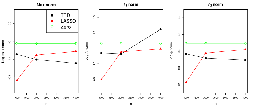
Figure 1: The log max, $\ell_{1}$, and $\ell_{2}$ norm error plots of the TED (black dot), LASSO (red triangle), and Zero (green diamond) estimators for a sample size $n=1000,2000,4000$.

In this paper, we develop a novel high-dimensional integrated coefficient estimator based on regression jump-diffusion processes contaminated by microstructure noises. To handle the high dimensionality and time-variation in the coefficient process, we impose a sparse structure on the coefficient process and assume that the coefficient process follows a diffusion process. Due to the time-varying property of the coefficient process, we first estimate the instantaneous coefficients. Specifically, since noises dominate a signal of the regression variables, we smooth the observed variables using a kernel function. Then, we perform a local regression procedure using the smoothed variables. Due to the noises, the direct application of the LASSO procedure to the smoothed variables cannot guarantee the deviation condition and leads to a nonconsistency. Thus, we adjust the bias in a loss function using the noise covariance matrix estimator and employ $\ell_{1}$-regularization to accommodate the sparsity of the coefficient process. Due to the bias adjustment, it becomes a nonconvex optimization problem. We demonstrate that the resulting instantaneous coefficient estimator achieves the desirable convergence rate. However, the instantaneous coefficient estimator is biased due to the $\ell_{1}$-regularization. To handle this bias, we employ a debiasing scheme and estimate the integrated coefficient using debiased instantaneous coefficient estimators. However, the debiasing scheme causes non-sparsity of the integrated coefficient estimates. To accommodate sparsity, the integrated coefficient estimator is further regularized. We call it the Thresholded dEbiased Nonconvex LASSO (TEN-LASSO) estimator. We show that the TEN-LASSO estimator has a near-optimal convergence rate. Finally, to implement nonconvex optimization, we adopt the composite gradient descent method (Agarwal et al.,, 2012) and investigate its properties.

The rest of paper is organized as follows. Section 2 introduces the high-dimensional regression diffusion process. Section 3 proposes the TEN-LASSO estimator and establishes its concentration properties. In Section 4, we conduct a simulation study to check the finite sample performance of the proposed TEN-LASSO estimation procedure. In Section 5, we apply the proposed estimation procedure to high-frequency financial data. The conclusion is presented in Section 6, and we collect technical proofs in the Appendix.

2 The model setup

Let $Y(t)$ and $\mathbf{X}(t)=\left(X_{1}(t),\ldots,X_{p}(t)\right)^{\top}$ be the true dependent process and the vector of the true $p$-dimensional covariate process, respectively. We consider the regression diffusion model as follows:

$$dY(t)=dY^{c}(t)+dY^{J}(t),$$ (2.1)

$$dY^{c}(t)=\boldsymbol{\beta}^{\top}(t)d\mathbf{X}^{c}(t)+dZ(t),\quad\text{and}\quad dY^{J}(t)=J^{Y}(t)d\Lambda^{Y}(t),$$ (2.2)

where $Y^{c}(t)$ and $Y^{J}(t)$ denote the continuous part and jump part of $Y(t)$, respectively, $J^{Y}(t)$ is a jump size process, $\Lambda^{Y}(t)$ is a Poisson process with a bounded intensity, $\mathbf{X}^{c}(t)=\left(X^{c}_{1}(t),\ldots,X^{c}_{p}(t)\right)^{\top}$ is the continuous part of $\mathbf{X}(t)$, $\boldsymbol{\beta}(t)=\left(\beta_{1}(t),\ldots,\beta_{p}(t)\right)^{\top}$ is a coefficient process, and $Z(t)$ is a residual process. The superscripts $c$ and $J$ represent the continuous and jump parts of the process, respectively. The true covariate process $\mathbf{X}(t)$ and residual process $Z(t)$ satisfy

$$d\mathbf{X}(t)=d\mathbf{X}^{c}(t)+d\mathbf{X}^{J}(t),\quad d\mathbf{X}^{c}(t)=\boldsymbol{\mu}(t)dt+\boldsymbol{\sigma}(t)d\mathbf{W}(t),$$ (2.3)

$$d\mathbf{X}^{J}(t)=\mathbf{J}(t)d\boldsymbol{\Lambda}(t),\quad\text{and}\quad dZ(t)=\nu(t)dB(t),$$ (2.4)

where $\mathbf{X}^{J}(t)$ denotes the jump part of $\mathbf{X}(t)$, $\mathbf{J}(t)=\left(J_{1}(t),\ldots,J_{p}(t)\right)^{\top}$ is a jump process, $\boldsymbol{\Lambda}(t)=\left(\Lambda_{1}(t),\ldots,\Lambda_{p}(t)\right)^{\top}$ denotes a $p$-dimensional Poisson process with the bounded intensity processes, $\boldsymbol{\mu}(t)$ is a drift process, $\boldsymbol{\sigma}(t)$ is a $p$ by $q_{1}$ instantaneous volatility matrix process, and $\nu(t)$ is a one-dimensional instantaneous volatility process. The processes $\boldsymbol{\mu}(t)$, $\boldsymbol{\sigma}(t)$, $\nu(t)$, and $\boldsymbol{\beta}(t)$ are predictable, and $\mathbf{W}(t)$ and $B(t)$ are $q_{1}$-dimensional and one-dimensional independent Brownian motions, respectively. The coefficient process $\boldsymbol{\beta}(t)$ satisfies the following diffusion model:

$$d\boldsymbol{\beta}(t)=\boldsymbol{\mu}_{\beta}(t)dt+\boldsymbol{\nu}_{\beta}(t)d\mathbf{W}_{\beta}(t),$$

where $\boldsymbol{\mu}_{\beta}(t)$ is a drift process, $\boldsymbol{\nu}_{\beta}(t)$ is a $p$ by $q_{2}$ instantaneous volatility matrix process, $\boldsymbol{\mu}_{\beta}(t)$ and $\boldsymbol{\nu}_{\beta}(t)$ are predictable, and $\mathbf{W}_{\beta}(t)$ is a $q_{2}$-dimensional independent Brownian motion. In this paper, the parameter of interest is the following integrated coefficient:

$$I\beta=(I\beta_{j})_{j=1,\ldots,p}=\int_{0}^{1}\boldsymbol{\beta}(t)dt.$$

In financial practices, there exist hundreds of potential factor candidates (Bali et al.,, 2011; Campbell et al.,, 2008; Cochrane,, 2011; Harvey et al.,, 2016; Hou et al.,, 2020; McLean and Pontiff,, 2016). To accommodate the large set of factor candidates, we assume that the dimension of the covariate process, $p$, is large, which causes the curse of dimensionality. To handle this issue, we impose the exact sparsity condition for the coefficient process. That is, there exists a set $S\subset\{1,\ldots,p\}$ with cardinality at most $s_{p}$ such that $\beta_{j}(t)=0$ for $0\leq t\leq 1$ and $j\notin S$.

Unfortunately, we cannot observe the true processes $\mathbf{X}(t)$ and $Y(t)$, since the high-frequency data are contaminated by microstructure noises. These noises result from market inefficiencies, such as the bid-ask spread, rounding effect, and asymmetric information. To account for this feature, we assume that the observed processes satisfy

$$Y^{o}(t_{i})=Y(t_{i})+\epsilon^{Y}(t_{i})\quad\text{ for }i=0,\ldots,n,\quad\text{ and}$$ (2.5)

$$\mathbf{X}^{o}(t_{i})=\mathbf{X}(t_{i})+\boldsymbol{\varepsilon}^{X}(t_{i})\quad\text{ for }i=0,\ldots,n,$$ (2.6)

where $t_{i}\in[0,1]$ is the $i$th observation time point, $Y^{o}(t_{i})$ is the observed dependent process for time $t_{i}$, $\mathbf{X}^{o}(t_{i})=\left(X_{1}^{o}(t_{i}),\ldots,X_{p}^{o}(t_{i})\right)^{\top}$ is the observed covariate process for time $t_{i}$, and $\epsilon^{Y}(t_{i})$ and $\boldsymbol{\varepsilon}^{X}(t_{i})=\left(\epsilon^{X}_{1}(t_{i}),\ldots,\epsilon^{X}_{p}(t_{i})\right)^{\top}$ are one-dimensional and $p$-dimensional microstructure noises for $Y(t_{i})$ and $\mathbf{X}(t_{i})$, respectively. The noises are independent over time and have a mean of zero and variances of $\operatorname{E}\{\epsilon^{Y}(t_{i})\}^{2}=V^{Y}$ and $\operatorname{E}\left\{\boldsymbol{\varepsilon}^{X}(t_{i})\left(\boldsymbol{\varepsilon}^{X}(t_{i})\right)^{\top}\right\}=\mathbf{V}^{X}$, where $\mathbf{V}^{X}=\left(V^{X}_{jj^{\prime}}\right)_{1\leq j,j^{{}^{\prime}}\leq p}$. For simplicity, we assume that the observation time points are synchronized and equally spaced: $t_{i}-t_{i-1}=1/n$ for $i=1,\ldots,n$.

Remark 1.

We can relax the conditions for the observation time points by employing the generalized sampling time (Aït-Sahalia et al.,, 2010), refresh time (Barndorff-Nielsen et al.,, 2011), and previous tick (Zhang,, 2011) schemes. Then, the above condition can be extended to the non-synchronized and unequally spaced condition. In this paper, we focus on developing an integrated coefficient estimation method; therefore, we assume the synchronized and equally spaced observation time condition for simplicity.

3 Nonconvex high-dimensional high-frequency regression

3.1 Integrated coefficient estimation procedure

In this section, we propose a high-dimensional integrated coefficient estimation procedure in the presence of microstructure noises and jumps. We first fix some notations. For any $p_{1}$ by $p_{2}$ matrix $\mathbf{G}=\left(G_{ij}\right)$, define

$$\|\mathbf{G}\|_{1}=\max\limits_{1\leq j\leq p_{2}}\sum\limits_{i=1}^{p_{1}}|G_{ij}|,\quad\|\mathbf{G}\|_{\infty}=\max\limits_{1\leq i\leq p_{1}}\sum\limits_{j=1}^{p_{2}}|G_{ij}|,\quad\text{ and }\quad\|\mathbf{G}\|_{\max}=\max_{i,j}|G_{ij}|.$$

We denote the Frobenius norm by $\|\mathbf{G}\|_{F}=\sqrt{\mathrm{tr}(\mathbf{G}^{\top}\mathbf{G})}$, and the matrix spectral norm $\|\mathbf{G}\|_{2}$ is denoted by the square root of the largest eigenvalue of $\mathbf{G}\mathbf{G}^{\top}$. For any process $f(t)$ and $\Delta_{n}=1/n$, define $\Delta_{i}^{n}f=f(i\Delta_{n})-f((i-1)\Delta_{n})$ for $1\leq i\leq n$. We use the subscript 0 to represent the true parameters. We use $C$’s to denote generic positive constants whose values are free of $n$ and $p$ and may vary from appearance to appearance.

Recently, Kim and Shin, (2022) developed an integrated coefficient estimator that can handle the high dimensionality and time-variation in the coefficient process without microstructure noises. However, in practice, when employing higher-frequency observations, microstructure noises tend to be observed. To accommodate these noises, we impose the noise structure as in (2.5). Based on the noisy high-frequency observation structure, we propose an integrated coefficient estimation procedure as follows. Due to the time-variation in the coefficient process, we first need to estimate the instantaneous coefficients. To handle the high dimensionality of instantaneous coefficients, we usually employ the penalized regression method for the observed log-returns, $\Delta_{i}^{n}Y^{o}$ and $\Delta_{i}^{n}\mathbf{X}^{o}$ (Kim and Shin,, 2022; Shin and Kim,, 2023). However, in the presence of noises, the noises dominate a signal of the true log-returns. This relationship ruins the regression structure in (2.1). To overcome this, we first construct smoothed variables for the observed processes. Specifically, let

$$\Delta_{i}^{n}\widehat{Y}=\sum^{k_{1}-1}_{l=0}g\left(\dfrac{l}{k_{1}}\right)\Delta_{i+l+1}^{n}Y^{o}\quad\text{and}\quad\Delta_{i}^{n}\widehat{X}_{j}=\sum^{k_{1}-1}_{l=0}g\left(\dfrac{l}{k_{1}}\right)\Delta_{i+l+1}^{n}X^{o}_{j},$$

where the kernel function $g(x)$ is Lipschitz continuous and satisfies $g(0)=g(1)=0$ and $\int_{0}^{1}\{g(t)\}^{2}dt>0$, and $k_{1}$ is the bandwidth parameter for $g(x)$. We choose $k_{1}=c_{k,1}n^{1/2}$ for some constant $c_{k,1}$, which ensures that the signals of the continuous underlying log-return and the noise are of the same magnitude. Thus, this bandwidth choice provides the optimal rate. Then, we employ a local regression with the smoothed variables as follows. Define

$$\mathcal{Y}_{i}=\begin{pmatrix}\Delta_{i}^{n}\widehat{Y}^{\text{trunc}}\\ \Delta_{i+1}^{n}\widehat{Y}^{\text{trunc}}\\ \vdots\\ \Delta_{i+k_{2}-k_{1}}^{n}\widehat{Y}^{\text{trunc}}\end{pmatrix}\quad\text{ and }\quad\mathcal{X}_{i}=\begin{pmatrix}\left(\Delta_{i}^{n}\widehat{\mathbf{X}}^{\text{trunc}}\right)^{\top}\\ \left(\Delta_{i+1}^{n}\widehat{\mathbf{X}}^{\text{trunc}}\right)^{\top}\\ \vdots\\ \left(\Delta_{i+k_{2}-k_{1}}^{n}\widehat{\mathbf{X}}^{\text{trunc}}\right)^{\top}\end{pmatrix},$$

where $k_{2}$ is the number of observed log-returns used for each local regression,

$$\Delta_{i}^{n}\widehat{Y}^{\text{trunc}}=\Delta_{i}^{n}\widehat{Y}\,\boldsymbol{1}\left(|\Delta_{i}^{n}\widehat{Y}|\leq u_{n}\right),\quad\Delta_{i}^{n}\widehat{\mathbf{X}}^{\text{trunc}}=\left(\Delta_{i}^{n}\widehat{X}_{j}^{\text{trunc}}\right)_{j=1,\ldots,p},$$

$$\Delta_{i}^{n}\widehat{X}_{j}^{\text{trunc}}=\Delta_{i}^{n}\widehat{X}_{j}\,\boldsymbol{1}\left(|\Delta_{i}^{n}\widehat{X}_{j}|\leq v_{j,n}\right),$$

$\boldsymbol{1}\left(\cdot\right)$ is an indicator function, and $u_{n}$ and $v_{j,n}$, $j=1,\ldots,p$, are the truncation parameters to handle the jumps. We choose $k_{2}=c_{k,2}n^{3/4}$ for some constant $c_{k,2}$. In addition, we choose

$$u_{n}=C_{u}s_{p}\sqrt{\log p}n^{-1/4}\quad\text{ and }\quad v_{j,n}=C_{j,v}\sqrt{\log p}n^{-1/4}$$ (3.1)

for some large constants $C_{u}$ and $C_{j,v}$, $j=1,\ldots,p$.

Remark 2.

The truncation parameters $u_{n}$ and $v_{j,n}$ control the information of the continuous processes by detecting and truncating the jumps. To detect the jumps, we need the conditions $u_{n}\geq Cs_{p}\sqrt{\log p}n^{-1/4}$ and $v_{j,n}\geq C\sqrt{\log p}n^{-1/4}$. The $\log p$ term is required to bound the continuous parts of the dependent and covariate processes with high probability. The $s_{p}$ term in $u_{n}$ is the cost to handle the continuous parts of $s_{p}$ significant factors. However, the $s_{p}$ term is not required when $Y^{c}(t)$ follows a continuous Itô diffusion model with bounded drift and volatility processes, which is a common assumption for a single process. That is, we technically add the $s_{p}$ term to handle a diverging significant factor summation; however, in the numerical study, we assume that the summation of the factor part is bounded for simplicity. On the other hand, to obtain the deviation and restricted eigenvalue conditions, we require sharp $u_{n}$ and $v_{j,n}$. For example, to obtain the restricted eigenvalue condition, we need $\left(\max_{j}v_{j,n}\right)^{2}n^{1/4}\log p\rightarrow 0$ as $n,p\rightarrow\infty$. Thus, we choose $u_{n}$ and $v_{j,n}$ as outlined in (3.1).

For each local regression, we need to handle the curse of dimensionality. To do this, we often utilize a penalized regression method, such as LASSO (Tibshirani,, 1996) or Dantzig (Candes and Tao,, 2007), under the sparsity assumption. However, they cannot consistently estimate instantaneous coefficients due to the bias from the microstructure noises. For example, the usual LASSO leads to the following instantaneous coefficient estimator at time $i\Delta_{n}$:

$$\widehat{\boldsymbol{\beta}}_{i\Delta_{n}}^{\text{LASSO}}=\underset{\boldsymbol{\beta}\in\mathbb{R}^{p}}{\operatorname{arg\,min}}\,\dfrac{n}{k_{1}k_{2}}\left\|\mathcal{Y}_{i}-\mathcal{X}_{i}\boldsymbol{\beta}\right\|^{2}_{2}+\eta\left\|\boldsymbol{\beta}\right\|_{1},$$

where $\eta>0$ is some regularization parameter. To obtain the consistency of $\widehat{\boldsymbol{\beta}}_{i\Delta_{n}}^{\text{LASSO}}$, we need the deviation condition $\dfrac{n}{k_{1}k_{2}}\|\mathcal{X}_{i}^{\top}\mathcal{X}_{i}\boldsymbol{\beta}-\mathcal{X}_{i}^{\top}\mathcal{Y}_{i}\|_{\max}\overset{p}{\to}0$. However, in the presence of noises, this condition cannot be satisfied, since $\operatorname{E}\left(\mathcal{X}_{i}^{\top}\mathcal{X}_{i}\right)$ contains noise covariance terms. Thus, we need to estimate the noise covariance matrix and adjust the bias. The noise covariance matrix is estimated by

$$\widehat{\mathbf{V}}^{X}=\dfrac{1}{2n}\sum_{i=1}^{n}\Delta_{i}^{n}\mathbf{X}^{\text{trunc}}\left(\Delta_{i}^{n}\mathbf{X}^{\text{trunc}}\right)^{\top},$$ (3.2)

where

$$\Delta_{i}^{n}\mathbf{X}^{\text{trunc}}=\left(\Delta_{i}^{n}X_{j}^{o}\,\boldsymbol{1}\left(|\Delta_{i}^{n}X_{j}^{o}|\leq v^{(2)}_{j,n}\right)\right)_{j=1,\ldots,p}$$

and $v^{(2)}_{j,n}$, $j=1,\ldots,p$, are the truncation parameters to handle the jumps. We utilize

$$v^{(2)}_{j,n}=C^{(2)}_{j,v}\sqrt{\log p}$$ (3.3)

for some large constants $C^{(2)}_{j,v}$, $j=1,\ldots,p$.

Remark 3.

As in (3.1), the truncation parameter $v^{(2)}_{j,n}$ controls the information for the noise covariances by detecting and truncating the jumps. To detect the jumps, the condition $v^{(2)}_{j,n}\geq C\sqrt{\log p}$ is required, which is different from the case of (3.1), since we only need to estimate the noise covariance matrix using the observed log-returns. We note that the $\log p$ term is required to bound the noise part with high probability. On the other hand, we need $\left(\max_{j}v_{j,n}^{(2)}\right)^{2}\log p/n\rightarrow 0$ as $n,p\rightarrow\infty$ to satisfy the restricted eigenvalue condition. Thus, we choose sharp $v_{j,n}^{(2)}$, as in (3.3). It is worth noting that when the jump size is finite, truncation for the observed log-returns is not required. However, since we do not impose any assumption on the jump size process, the proposed truncation method is used to handle the heavy-tailedness of the jump sizes.

Then, the instantaneous coefficient estimator at time $i\Delta_{n}$ is defined as follows:

$$\widehat{\boldsymbol{\beta}}_{i\Delta_{n}} = \underset{\|\boldsymbol{\beta}\|_{1}\leq r}{\operatorname{arg\,min}}\,{\mathcal{L}}_{i}(\boldsymbol{\beta})+\eta\left\|\boldsymbol{\beta}\right\|_{1},$$ (3.4)

$${\mathcal{L}}_{i}(\boldsymbol{\beta}) = \dfrac{n}{2\phi k_{1}k_{2}}\|\mathcal{Y}_{i}-\mathcal{X}_{i}\boldsymbol{\beta}\|_{2}^{2}-\dfrac{n\zeta}{2\phi k_{1}}\boldsymbol{\beta}^{\top}\widehat{\mathbf{V}}^{X}\boldsymbol{\beta},$$ (3.5)

where $r$ satisfies $r\geq\|\boldsymbol{\beta}_{0}(i\Delta_{n})\|_{1}$, $\eta>0$ is the regularization parameter, ${\mathcal{L}}_{i}(\boldsymbol{\beta})$ is the empirical loss function, $\phi=\frac{1}{k_{1}}\sum_{\ell=0}^{k_{1}-1}\left\{g\left(\frac{\ell}{k_{1}}\right)\right\}^{2}$, and $\zeta=\sum\limits_{l=0}^{k_{1}-1}\left\{g\left(\frac{l}{k_{1}}\right)-g\left(\frac{l+1}{k_{1}}\right)\right\}^{2}=O\left(\frac{1}{k_{1}}\right)$. The tuning parameters $r$ and $\eta$ will be specified in Theorem 1. We note that the Hessian matrix of the empirical loss function, $\nabla^{2}{\mathcal{L}}_{i}(\boldsymbol{\beta})=\dfrac{n}{\phi k_{1}k_{2}}\mathcal{X}_{i}^{\top}\mathcal{X}_{i}-\dfrac{n\zeta}{\phi k_{1}}\widehat{\mathbf{V}}^{X}$, has the same form as the pre-averaging realized volatility (PRV) (Christensen et al.,, 2010; Jacod et al.,, 2009), which can be one of the estimators for the instantaneous volatility matrix $\boldsymbol{\Sigma}(t)=\boldsymbol{\sigma}(t)\boldsymbol{\sigma}^{\top}(t)$. Thus, the deviation condition is satisfied. However, we cannot guarantee that $\nabla^{2}{\mathcal{L}}_{i}(\boldsymbol{\beta})$ is positive semidefinite due to the bias adjustment, which implies that the objective function ${\mathcal{L}}_{i}(\boldsymbol{\beta})+\eta\left\|\boldsymbol{\beta}\right\|_{1}$ can be unbounded from below. To handle the unbounded problem, we impose the constraint on $\boldsymbol{\beta}$, such as $\|\boldsymbol{\beta}\|_{1}\leq r$, for the nonconvex optimization problem (3.4). Theorem 1 shows that the instantaneous coefficient estimator $\widehat{\boldsymbol{\beta}}_{i\Delta_{n}}$ is consistent when we choose appropriate $r$ and $\eta$.

To estimate the integrated coefficient, we can consider the integration of $\widehat{\boldsymbol{\beta}}_{i\Delta_{n}}$’s. However, $\widehat{\boldsymbol{\beta}}_{i\Delta_{n}}$’s are biased due to the regularization, so their integration fails to enjoy the law of large number property. In other words, the integration has the same convergence rate as $\widehat{\boldsymbol{\beta}}_{i\Delta_{n}}$. To obtain a faster convergence rate, we apply the debiasing scheme to each $\widehat{\boldsymbol{\beta}}_{i\Delta_{n}}$ as follows. We first estimate the inverse instantaneous volatility matrix $\boldsymbol{\Omega}_{0}(i\Delta_{n})=\boldsymbol{\Sigma}_{0}^{-1}(i\Delta_{n})$ based on the following constrained $\ell_{1}$-minimization for inverse matrix estimation (CLIME) (Cai et al.,, 2011):

$$\widehat{\boldsymbol{\Omega}}_{i\Delta_{n}}=\arg\min\|\boldsymbol{\Omega}\|_{1}\quad\text{s.t.}\quad\left\|\left(\dfrac{n}{\phi k_{1}k_{2}}\mathcal{X}_{i}^{\top}\mathcal{X}_{i}-\dfrac{n\zeta}{\phi k_{1}}\widehat{\mathbf{V}}^{X}\right)\boldsymbol{\Omega}-\mathbf{I}\right\|_{\max}\leq\tau,$$ (3.6)

where $\tau$ is the tuning parameter that will be specified in Theorem 2. Using the inverse instantaneous volatility matrix estimator $\widehat{\boldsymbol{\Omega}}_{i\Delta_{n}}$, we adjust the instantaneous coefficient estimator $\widehat{\boldsymbol{\beta}}_{i\Delta_{n}}$ as follows:

$$\widetilde{\boldsymbol{\beta}}_{i\Delta_{n}}=\widehat{\boldsymbol{\beta}}_{i\Delta_{n}}+\dfrac{n}{\phi k_{1}k_{2}}\widehat{\boldsymbol{\Omega}}_{i\Delta_{n}}^{\top}\left\{\mathcal{X}_{i}^{\top}\mathcal{Y}_{i}-\left(\mathcal{X}_{i}^{\top}\mathcal{X}_{i}-k_{2}\zeta\widehat{\mathbf{V}}^{X}\right)\widehat{\boldsymbol{\beta}}_{i\Delta_{n}}\right\}.$$ (3.7)

We note that $\dfrac{n}{\phi k_{1}k_{2}}\mathcal{X}_{i}^{\top}\mathcal{X}_{i}-\dfrac{n\zeta}{\phi k_{1}}\widehat{\mathbf{V}}^{X}$ is the proxy for the instantaneous volatility matrix at time $i\Delta_{n}$. Then, we estimate the integrated coefficient as follows:

$$\widehat{I\beta}=\sum_{i=0}^{[1/(k_{2}\Delta_{n})]-1}\widetilde{\boldsymbol{\beta}}_{ik_{2}\Delta_{n}}k_{2}\Delta_{n}.$$ (3.8)

The debiased integrated coefficient estimator $\widehat{I\beta}$ can enjoy the law of large number property and has a faster convergence rate than the integration of the instantaneous coefficient estimators. However, the bias adjustment leads to the non-sparse structure of the integrated coefficient estimator. To accommodate the sparse structure of the integrated coefficient, we employ the thresholding scheme as follows:

$$\widetilde{I\beta}_{j}=s(\widehat{I\beta}_{j})\boldsymbol{1}\left(|\widehat{I\beta}_{j}|\geq h_{n}\right)\quad\text{and}\quad\widetilde{I\beta}=\left(\widetilde{I\beta}_{j}\right)_{j=1,\ldots,p},$$

where $s(x)$ is the thresholding function satisfying $|s(x)-x|\leq h_{n}$ and $h_{n}$ is a thresholding level that will be specified in Theorem 3. For the thresholding function $s(x)$, we usually employ the soft thresholding function $s(x)=x-\mbox{sign}(x)h_{n}$ or hard thresholding function $s(x)=x$. We utilize the hard thresholding function in the empirical study. We call this the Thresholded dEbiased Nonconvex LASSO (TEN-LASSO) estimator. A summary of the TEN-LASSO estimation procedure is presented in Algorithm 1. We will discuss the choice of the tuning parameters in Section 3.4.

Algorithm 1 TEN-LASSO estimation procedure

Step 1 Obtain the noise covariance matrix estimator:

$$\widehat{\mathbf{V}}^{X}=\dfrac{1}{2n}\sum_{i=1}^{n}\Delta_{i}^{n}\mathbf{X}^{\text{trunc}}\left(\Delta_{i}^{n}\mathbf{X}^{\text{trunc}}\right)^{\top}.$$

Step 2 Estimate the instantaneous coefficient:

$$\widehat{\boldsymbol{\beta}}_{i\Delta_{n}}=\underset{\|\boldsymbol{\beta}\|_{1}\leq r}{\operatorname{arg\,min}}\,\dfrac{n}{2\phi k_{1}k_{2}}\|\mathcal{Y}_{i}-\mathcal{X}_{i}\boldsymbol{\beta}\|_{2}^{2}-\dfrac{n\zeta}{2\phi k_{1}}\boldsymbol{\beta}^{\top}\widehat{\mathbf{V}}^{X}\boldsymbol{\beta}+\eta\left\|\boldsymbol{\beta}\right\|_{1},$$

where $r=C_{r}s_{p}$, $k_{1}=c_{k_{1}}n^{1/2}$, $k_{2}=c_{k_{2}}n^{3/4}$, and $\eta=C_{\eta}s_{p}n^{-1/8}\left(\log p\right)^{3/2}$ for some constants $C_{r}$, $c_{k_{1}}$, $c_{k_{2}}$, and $C_{\eta}$.

Step 3 Estimate the inverse instantaneous volatility matrix:

$$\widehat{\boldsymbol{\Omega}}_{i\Delta_{n}}=\arg\min\|\boldsymbol{\Omega}\|_{1}\quad\text{s.t.}\quad\left\|\left(\dfrac{n}{\phi k_{1}k_{2}}\mathcal{X}_{i}^{\top}\mathcal{X}_{i}-\dfrac{n\zeta}{\phi k_{1}}\widehat{\mathbf{V}}^{X}\right)\boldsymbol{\Omega}-\mathbf{I}\right\|_{\max}\leq\tau,$$

where $\tau=C_{\tau}n^{-1/8}\sqrt{\log p}$ for some large constant $C_{\tau}$.

Step 4 Obtain the debiased instantaneous coefficient estimator:

$$\widetilde{\boldsymbol{\beta}}_{i\Delta_{n}}=\widehat{\boldsymbol{\beta}}_{i\Delta_{n}}+\dfrac{n}{\phi k_{1}k_{2}}\widehat{\boldsymbol{\Omega}}_{i\Delta_{n}}^{\top}\left\{\mathcal{X}_{i}^{\top}\mathcal{Y}_{i}-\left(\mathcal{X}_{i}^{\top}\mathcal{X}_{i}-k_{2}\zeta\widehat{\mathbf{V}}^{X}\right)\widehat{\boldsymbol{\beta}}_{i\Delta_{n}}\right\}.$$

Step 5 Obtain the debiased integrated coefficient estimator:

$$\widehat{I\beta}=\sum_{i=0}^{[1/(k_{2}\Delta_{n})]-1}\widetilde{\boldsymbol{\beta}}_{ik_{2}\Delta_{n}}k_{2}\Delta_{n}.$$

Step 6 Threshold the debiased integrated coefficient estimator:

$$\widetilde{I\beta}_{j}=s(\widehat{I\beta}_{j})\boldsymbol{1}\left(|\widehat{I\beta}_{j}|\geq h_{n}\right)\quad\text{and}\quad\widetilde{I\beta}=\left(\widetilde{I\beta}_{j}\right)_{j=1,\ldots,p},$$

where $s(x)$ satisfies $|s(x)-x|\leq h_{n}$ and $h_{n}=C_{h}\left\{s_{p}^{2}n^{-1/4}\left(\log p\right)^{2}+s_{p}s_{\omega,p}n^{\left(-2+q\right)/8}\left(\log p\right)^{\left(4-q\right)/2}\right\}$ for some large constant $C_{h}$.

3.2 Theoretical results

In this section, we show the asymptotic properties of the proposed TEN-LASSO estimator. To investigate its asymptotic behaviors, the following assumptions are required.

Assumption 1.

• $\boldsymbol{\mu}(t)$, $\boldsymbol{\Sigma}(t)$, $\boldsymbol{\beta}(t)$, $\boldsymbol{\mu}_{\beta}(t)$, and $\boldsymbol{\Sigma}_{\beta}(t)=\boldsymbol{\nu}_{\beta}(t)\boldsymbol{\nu}_{\beta}^{\top}(t)$ are almost surely entry-wise bounded, and $\|\boldsymbol{\Sigma}^{-1}(t)\|_{1}\leq C$ a.s.

• The noises $\epsilon_{j}^{X}(t_{i})$, $j=1,\ldots,p$, and $\epsilon^{Y}(t_{i})$ are sub-Gaussian with a bounded parameter.

• For $\mathbf{b}=\left(1,\ldots,1\right)^{\top}\in\mathbb{R}^{p}$, the random variable $\left(\mathbf{b}^{\top}\int_{i\Delta_{n}}^{(i+k_{2})\Delta_{n}}d\boldsymbol{\Lambda}(t)dt\right)$ is sub-exponential with a bounded parameter. The largest eigenvalue of $\boldsymbol{\Sigma}(t)$, $\lambda_{max}\left\{\boldsymbol{\Sigma}(t)\right\}$, is bounded.

• The volatility matrix process $\boldsymbol{\Sigma}(t)=(\Sigma_{ij}(t))_{i,j=1,\ldots,p}$ satisfies the following Hölder condition:

  $$|\Sigma_{ij}(t)-\Sigma_{ij}(s)|\leq C\sqrt{|t-s|\log p}\,\text{ a.s.}$$

• $n^{c_{1}}\leq p\leq\exp(n^{c_{2}})$ for some positive constants $c_{1}$ and $c_{2}$, and $s_{p}n^{-1/8}\left(\log p\right)^{3/2}\rightarrow 0$ as $n,p\rightarrow\infty$.

• The inverse volatility matrix process, $\boldsymbol{\Sigma}^{-1}(t)=\boldsymbol{\Omega}(t)=(\omega_{ij}(t))_{i,j=1,\ldots,p}$, satisfies the following sparsity condition for $q\in[0,1)$:

  $$\sup_{0\leq t\leq 1}\max_{1\leq i\leq p}\sum_{j=1}^{p}|\omega_{ij}(t)|^{q}\leq s_{\omega,p}\,\text{ a.s.},$$

  where $s_{\omega,p}$ grows slowly in $p$, for example, $\log p$.

Remark 4.

Assumption 1(a) is the boundedness condition, which implies the sub-Gaussian tails for the continuous part of the covariate process $\mathbf{X}(t)$ and the coefficient process $\boldsymbol{\beta}(t)$. Sub-Gaussianity is often imposed to investigate high-dimensional inferences. On the other hand, we can relax the boundedness condition to the locally boundedness condition using Lemma 4.4.9 in Jacod and Protter, (2011). It states that if an asymptotic property, such as stable convergence in law or convergence in probability, is obtained under the boundedness condition, it can also be obtained under the locally boundedness condition. Thus, the boundedness condition is not restrictive. Similarly, in Assumption 1(b), we impose sub-Gaussianity for the noises. Assumption 1(c) is the technical condition, which is required to obtain the restricted eigenvalue condition for the LASSO-type estimator. Assumption 1(d) is the continuity condition, which is required to investigate the asymptotic properties of the estimators for the time-varying processes. This condition can be obtained with high probability when the volatility process $\boldsymbol{\Sigma}(t)$ follows a continuous Itô diffusion model with bounded drift and volatility processes. Finally, we impose the sparse structure on the inverse volatility matrix process to investigate the asymptotic behaviors of the CLIME estimator.

The following theorem establishes the asymptotic behaviors of the instantaneous coefficient estimator $\widehat{\boldsymbol{\beta}}_{i\Delta_{n}}$.

Theorem 1.

Under the models (2.1)–(2.5) and Assumption 1(a)–(e), let $k_{1}=c_{k_{1}}n^{1/2}$ and $k_{2}=c_{k_{2}}n^{3/4}$ for some constants $c_{k_{1}}$ and $c_{k_{2}}$. For any given positive constant $a$, choose $r=C_{r,a}s_{p}$ and $\eta=C_{\eta,a}s_{p}n^{-1/8}\left(\log p\right)^{3/2}$ for some large constants $C_{r,a}$ and $C_{\eta,a}$. Then, we have, for large $n$,

$$\max_{i}\|\widehat{\boldsymbol{\beta}}_{i\Delta_{n}}-\boldsymbol{\beta}_{0}(i\Delta_{n})\|_{1}\leq Cs_{p}\eta\quad\text{and}\quad\max_{i}\|\widehat{\boldsymbol{\beta}}_{i\Delta_{n}}-\boldsymbol{\beta}_{0}(i\Delta_{n})\|_{2}\leq C\sqrt{s_{p}}\eta,$$ (3.9)

with the probability at least $1-p^{-a}$.

Remark 5.

Theorem 1 shows that the instantaneous coefficient estimator has the convergence rate of $n^{-1/8}$ with the sparsity-level and log order terms. We note that for each local regression, the number of observed log-returns is $Cn^{3/4}$, whereas the number of non-overlapping smoothed variables is $Cn^{1/4}$. That is, due to the cost of managing the noises, we are able to use only $Cn^{1/4}$ variables to estimate the instantaneous coefficient. Thus, the optimal convergence rate is expected to be $n^{-1/8}$. From this point of view, the proposed instantaneous coefficient estimator achieves the desirable convergence rate.

As discussed in Section 3.1, the instantaneous coefficient estimators are biased due to the regularization. Thus, the integration of the instantaneous coefficient estimators cannot enjoy the law of large number property. To handle this issue, we utilized the debiasing scheme and obtain the debiased integrated coefficient estimator, as outlined in (3.7) and (3.8). We establish the asymptotic property of the debiased integrated coefficient estimator in the following theorem.

Theorem 2.

Under the assumptions in Theorem 1 and Assumption 1(f), for any given positive constant $a$, choose $\tau=C_{\tau,a}n^{-1/8}\sqrt{\log p}$ for some constant $C_{\tau,a}$. Then, we have, with the probability at least $1-p^{-a}$,

$$\|\widehat{I\beta}-I\beta_{0}\|_{\max}\leq Cb_{n},$$ (3.10)

where $b_{n}=\left\{s_{p}^{2}n^{-1/4}\left(\log p\right)^{2}+s_{p}s_{\omega,p}n^{\left(-2+q\right)/8}\left(\log p\right)^{\left(4-q\right)/2}\right\}$.

Remark 6.

Theorem 2 indicates that the debiased integrated coefficient estimator is consistent in terms of the max norm. When the inverse volatility matrix process satisfies the exact sparsity condition, that is, $q=0$, the debiased integrated coefficient estimator has the convergence rate of $n^{-1/4}\left(s_{p}+s_{\omega,p}\right)s_{p}\left(\log p\right)^{2}$. In contrast, we have the convergence rate of $n^{-1/8}s_{p}^{2}\left(\log p\right)^{3/2}$ without a debiasing scheme. In high-dimensional statistics, the sparsity-level is assumed to diverge relatively slowly, such as $\log p$. Thus, the debiased integrated coefficient estimator has the faster convergence rate than the integration of the instantaneous coefficient estimators.

Theorem 2 shows that we can obtain well-performing input-integrated coefficient estimator $\widehat{I\beta}$ with the debiasing scheme. Finally, to accommodate the sparse structure, we utilize the thresholding scheme and obtain the TEN-LASSO estimator. The following theorem provides the $\ell_{1}$ convergence rate of the TEN-LASSO estimator.

Theorem 3.

Under the assumptions in Theorems 1 and 2, for any given positive constant $a$, choose $h_{n}=C_{h,a}b_{n}$ for some constant $C_{h,a}$, where $b_{n}$ is defined in Theorem 2. Then, we have, with probability at least $1-p^{-a}$,

$$\|\widetilde{I\beta}-I\beta_{0}\|_{1}\leq Cs_{p}b_{n}.$$ (3.11)

Theorem 3 shows the $\ell_{1}$ norm error bound of the proposed TEN-LASSO estimator. When the exact sparsity condition is satisfied, that is, $q=0$, the TEN-LASSO estimator has the convergence rate of $n^{-1/4}\left(s_{p}+s_{\omega,p}\right)s_{p}^{2}\left(\log p\right)^{2}$. We note that in the presence of microstructure noises, $n^{-1/4}$ is the optimal convergence rate of the integrated coefficient estimator in the finite-dimensional setup. Thus, the TEN-LASSO estimator achieves the optimal convergence rate with up to $\log p$ and sparsity-level orders.

3.3 Implementation of the TEN-LASSO estimation procedure

To implement the TEN-LASSO estimation procedure, we need to solve the nonconvex optimization problem (3.4). However, it is generally hard to obtain the global minimizer of the nonconvex optimization problem in a polynomial time. To handle this issue, we employ the composite gradient descent method (Agarwal et al.,, 2012) as follows:

$$\widehat{\boldsymbol{\beta}}_{i\Delta_{n}}^{t+1}=\underset{\left\|\boldsymbol{\beta}\right\|_{1}\leq r}{\operatorname{arg\,min}}\left\{\mathcal{L}_{i}\left(\widehat{\boldsymbol{\beta}}_{i\Delta_{n}}^{t}\right)+\langle\nabla{\mathcal{L}}_{i}(\widehat{\boldsymbol{\beta}}_{i\Delta_{n}}^{t}),\boldsymbol{\beta}-\widehat{\boldsymbol{\beta}}_{i\Delta_{n}}^{t}\rangle+\alpha_{2}\left\|\boldsymbol{\beta}-\widehat{\boldsymbol{\beta}}_{i\Delta_{n}}^{t}\right\|_{2}^{2}+\eta\left\|\boldsymbol{\beta}\right\|_{1}\right\},$$ (3.12)

where $\widehat{\boldsymbol{\beta}}_{i\Delta_{n}}^{0}$ is the initial parameter, and $\alpha_{2}>0$ is defined in Proposition 3 in the Appendix. Then, we can obtain the following proposition.

Proposition 1.

Under the assumptions in Theorem 1, we have, with the probability at least $1-p^{-a}$,

$$\max_{i}\|\widehat{\boldsymbol{\beta}}_{i\Delta_{n}}^{t}-\widehat{\boldsymbol{\beta}}_{i\Delta_{n}}\|_{2}\leq C\sqrt{s_{p}}\eta$$ (3.13)

for all $t\geq C\left\{\log\left(\dfrac{\phi_{i}(\widehat{\boldsymbol{\beta}}_{i\Delta_{n}}^{0})-\phi_{i}(\widehat{\boldsymbol{\beta}}_{i\Delta_{n}})}{\|\widehat{\boldsymbol{\beta}}_{i\Delta_{n}}-\boldsymbol{\beta}_{0}\left(i\Delta_{n}\right)\|_{2}^{2}}\right)+\log_{2}\log_{2}\left(\dfrac{Cs_{p}\eta}{\|\widehat{\boldsymbol{\beta}}_{i\Delta_{n}}-\boldsymbol{\beta}_{0}\left(i\Delta_{n}\right)\|_{2}^{2}}\right)\right\}$, where $\phi_{i}\left(\boldsymbol{\beta}\right)={\mathcal{L}}_{i}(\boldsymbol{\beta})+\eta\left\|\boldsymbol{\beta}\right\|_{1}$.

Proposition 1 shows that the $\ell_{2}$ distance between the local minimizer $\widehat{\boldsymbol{\beta}}_{i\Delta_{n}}^{t}$ and global minimizer $\widehat{\boldsymbol{\beta}}_{i\Delta_{n}}$ has the same convergence rate as the statistical error of the global minimizer $\widehat{\boldsymbol{\beta}}_{i\Delta_{n}}$. That is, the local and global minimizers have the same convergence rate in terms of the $\ell_{2}$ norm. Furthermore, the local minimizer $\widehat{\boldsymbol{\beta}}_{i\Delta_{n}}^{t}$ can be obtained in a polynomial time. Thus, the proposed TEN-LASSO procedure is computationally feasible with theoretical guarantees.

3.4 Discussion on tuning parameter selection

In this section, we discuss the process of selecting the tuning parameter for the TEN-LASSO estimator. To obtain the smoothed variables, we choose

$$g(x)=x\wedge(1-x)\,\,\,\text{ and }\,\,\,k_{1}=\dfrac{1}{2}\,n^{1/2}.$$

We select $k_{2}=n^{3/4}$ in the simulation study, and the selection of $k_{2}$ for the empirical study is described in Section 5. For the jump truncation parameters in (3.1) and (3.3), we use

$$u_{n}=3\,\text{sd}\left(\Delta_{i}^{n}\widehat{Y}\right),\,\,\,v_{j,n}=3\,\text{sd}\left(\Delta_{i}^{n}\widehat{X}_{j}\right),\,\,\,\text{ and }\,\,\,v_{j,n}^{(2)}=3\,\text{sd}\left(\Delta_{i}^{n}X_{j}^{o}\right),$$ (3.14)

where sd represents the sample standard deviation. Then, the variables $\Delta_{i}^{n}\widehat{Y}^{\text{trunc}}$ and $\Delta_{i}^{n}\widehat{X}_{j}^{\text{trunc}}$, $j=1,\ldots,p$, are standardized to have a mean of zero and a variance of 1. We conduct re-scaling after obtaining the TEN-LASSO estimator. For the nonconvex optimization, we implement the composite gradient descent method (3.12) with $10^{3}$ updates. We set $\widehat{\boldsymbol{\beta}}_{0}^{0}=\left(0,\ldots,0\right)^{\top}\in\mathbb{R}^{p}$ and $\widehat{\boldsymbol{\beta}}_{i\Delta_{n}}^{0}=\widehat{\boldsymbol{\beta}}_{(i-k_{2})\Delta_{n}}$ for $i\geq k_{2}$. That is, we set the initial parameter as the previous instantaneous coefficient estimator. We choose $\alpha_{2}$ as the largest eigenvalue of $\dfrac{n}{\phi k_{1}k_{2}}\mathcal{X}_{i}^{\top}\mathcal{X}_{i}$ and set $r=2\,\|\widehat{\boldsymbol{\beta}}^{\text{TEC}}_{i\Delta_{n}}\|_{1}$, where $\widehat{\boldsymbol{\beta}}^{\text{TEC}}_{i\Delta_{n}}$ is calculated using the usual LASSO procedure with the smoothed variables as follows:

$$\widehat{\boldsymbol{\beta}}^{\text{TEC}}_{i\Delta_{n}}={\operatorname{arg\,min}}\,\dfrac{n}{2\phi k_{1}k_{2}}\|\mathcal{Y}_{i}-\mathcal{X}_{i}\boldsymbol{\beta}\|_{2}^{2}+\eta^{\text{TEC}}\left\|\boldsymbol{\beta}\right\|_{1},$$ (3.15)

the regularization parameter $\eta^{\text{TEC}}=c_{\eta}^{\text{TEC}}n^{-1/8}\left(\log p\right)^{3/2}$, and $c_{\eta}^{\text{TEC}}\in[10^{-4},10^{4}]$ is chosen by minimizing the corresponding Bayesian information criterion (BIC). Furthermore, we select

$$\eta=c_{\eta}n^{-1/8}\left(\log p\right)^{3/2},\,\,\,\tau=c_{\tau}n^{-1/8}\sqrt{\log p},\,\,\,\text{and}\,\,\,h_{n}=c_{h}n^{-1/4}\left(\log p\right)^{2},$$ (3.16)

where $c_{\eta}$, $c_{\tau}$, and $c_{h}$ are the tuning parameters. We choose $c_{\eta}\in[10^{-4},10^{4}]$ by minimizing the corresponding Bayesian information criterion (BIC). We select $c_{\tau}\in[10^{-2},10^{2}]$, which minimizes the following loss function:

$$\operatorname{tr}\left[\left(\left\{\dfrac{n}{\phi k_{1}k_{2}}\mathcal{X}_{i}^{\top}\mathcal{X}_{i}-\dfrac{n\zeta}{\phi k_{1}}\widehat{\mathbf{V}}^{X}\right\}\widehat{\boldsymbol{\Omega}}_{i\Delta_{n}}-\mathbf{I}_{p}\right)^{2}\right],$$

where $\mathbf{I}_{p}$ is the $p$-dimensional identity matrix. Finally, $c_{h}$ is selected by minimizing the corresponding mean squared prediction error (MSPE). The result is $c_{h}=0.04$, and the specific procedure is described in Section 5.

4 A simulation study

In this section, we conducted a simulation study to check the finite sample performance of the TEN-LASSO estimator. The data were generated with a frequency of $1/n^{all}$ based on the following regression jump-diffusion model:

$$dY(t)=\boldsymbol{\beta}^{\top}(t)d\mathbf{X}^{c}(t)+dZ(t)+J^{y}(t)d\Lambda^{y}(t),\quad d\mathbf{X}(t)=d\mathbf{X}^{c}(t)+d\mathbf{X}^{J}(t),$$

$$d\mathbf{X}^{c}(t)=\boldsymbol{\sigma}(t)d\mathbf{W}(t),\quad d\mathbf{X}^{J}(t)=\mathbf{J}(t)d\boldsymbol{\Lambda}(t),\quad\text{and}\quad dZ(t)=\nu(t)dB(t),$$

where the jump sizes $J^{Y}(t)$ and $J_{j}(t)$ were generated from the independent normal distribution with a mean of zero and a standard deviation of $0.05$, and $\Lambda^{y}(t)$ and $\Lambda_{j}(t)$ were generated using Poisson processes with intensities of $20$ and $\left(15,\ldots,15\right)^{\top}$, respectively. The initial values $Y(0)$ and $X_{j}(0)$ were set as zero, and $\nu(t)$ was generated from the following Ornstein–Uhlenbeck process:

$$d\nu(t)=4\left(0.12-\nu(t)\right)dt+0.03dW^{\nu}(t),$$

where $\nu(0)=0.15$ and $W^{\nu}(t)$ is an independent Brownian motion. For the volatility process $\boldsymbol{\sigma}(t)$, we first generated the following Ornstein–Uhlenbeck process:

$$d\xi(t)=5\left(0.45-\xi(t)\right)dt+0.07dW^{\xi}(t),$$

where $\xi(0)=0.4$ and $W^{\xi}(t)$ is an independent Brownian motion. Then, $\boldsymbol{\sigma}(t)$ was taken to be a Cholesky decomposition of $\boldsymbol{\Sigma}(t)=(\Sigma_{ij}(t))_{1\leq i,j\leq p}$, where $\Sigma_{ij}(t)=\xi(t)0.3^{|i-j|}$. For the coefficient process $\boldsymbol{\beta}(t)$, we considered the following model:

$$d\boldsymbol{\beta}(t)=\boldsymbol{\mu}_{\beta}(t)dt+\boldsymbol{\nu}_{\beta}(t)d\mathbf{W}_{\beta}(t),$$

where $\boldsymbol{\mu}_{\beta}(t)=\left(\mu_{1,\beta}(t),\ldots,\mu_{p,\beta}(t)\right)^{\top}$ is a drift process, $\boldsymbol{\nu}_{\beta}(t)=\left(\nu_{i,j,\beta}(t)\right)_{1\leq i,j\leq p}$ is an instantaneous volatility matrix process, and $\mathbf{W}^{\beta}(t)$ is a $p$-dimensional independent Brownian motion. To generate $\boldsymbol{\nu}_{\beta}(t)$, we first generated the following Ornstein–Uhlenbeck process:

$$d\varphi(t)=3\left(0.25-\varphi(t)\right)dt+0.05dW_{t}^{\varphi},$$

where $\varphi(0)=0.15$ and $W_{t}^{\varphi}$ is an independent Brownian motion. Then, we set $\left(\nu_{i,j,\beta}(t)\right)_{1\leq i,j\leq s_{p}}$ as $\varphi(t)\mathbf{I}_{s_{p}}$, where $\mathbf{I}_{s_{p}}$ is the $s_{p}$-dimensional identity matrix. For $j=1,\ldots,s_{p}$, we took $\beta_{j}(0)=0.75$ and $\mu_{j,\beta}(t)=0.05$ for $0\leq t\leq 1$, whereas we set $\beta_{j}(t)=0$ for $j=s_{p}+1,\ldots,p$. Noise-contaminated high-frequency observations were generated as follows:

$$Y^{o}(t_{i})=Y(t_{i})+\epsilon^{Y}(t_{i})\quad\text{ for }i=0,\ldots,n,$$

$$\mathbf{X}^{o}(t_{i})=\mathbf{X}(t_{i})+\boldsymbol{\varepsilon}^{X}(t_{i})\quad\text{ for }i=0,\ldots,n,$$

where $\epsilon^{Y}(t_{i})$ and $\epsilon^{X}_{j}(t_{i})$ were obtained from an independent normal distribution with a mean of zero and a standard deviation of $0.05\sqrt{\int_{0}^{1}\boldsymbol{\beta}^{\top}(t)\boldsymbol{\sigma}(t)\boldsymbol{\sigma}^{\top}(t)\boldsymbol{\beta}(t)dt}$ and $0.05\sqrt{\int_{0}^{1}\Sigma_{jj}(t)dt}$, respectively. We set $p=100$, $s_{p}=[\log p]$, $n^{all}=4000$, and we varied $n$ from $1000$ to $4000$. To obtain the TEN-LASSO estimator, we employed the hard thresholding function $s\left(x\right)=x$ and implemented the tuning parameter choice procedure discussed in Section 3.4.

For the comparison, we employed the Thresholded dEbiased Convex LASSO (TEC-LASSO) estimator. It uses the same estimation procedure as the TEN-LASSO estimator, except for the bias adjustment for the noise covariance terms. Specifically, the instantaneous coefficient estimator for the TEC-LASSO procedure is defined in (3.15). We note that the TEC-LASSO estimator can partially explain the noises by using the smoothed variables. However, it cannot satisfy the deviation condition due to the bias from the noises, which leads to the non-consistency of the instantaneous coefficient estimator. We also considered the TED estimator (Kim and Shin,, 2022), which can handle the time-variation in the coefficient process and the curse of dimensionality. Specifically, with the observed log-returns, we first utilized the Dantzig selector (Candes and Tao,, 2007) to obtain the instantaneous coefficient estimator. Then, we employed debiasing and truncation schemes to obtain the integrated coefficient estimator. The detailed estimation procedure is presented in Algorithm 1 in Kim and Shin, (2022). Since the TED estimator directly uses the observed log-returns, it cannot account for the noises. Finally, we employed the LASSO estimator (Tibshirani,, 1996) as follows:

$$\widetilde{I\beta}^{{\rm LASSO}}=\operatorname{argmin}_{\boldsymbol{\beta}}\left\{\sum^{n-1}_{i=0}\left(\Delta_{i+1}^{n}Y^{\text{trunc2}}-\left(\Delta_{i+1}^{n}\mathbf{X}^{\text{trunc2}}\right)^{\top}\boldsymbol{\beta}\right)^{2}+\eta^{{\rm LASSO}}\|\boldsymbol{\beta}\|_{1}\right\},$$ (4.1)

where $\Delta_{i}^{n}Y^{\text{trunc2}}=\Delta_{i}^{n}Y^{o}\,\boldsymbol{1}\left(|\Delta_{i}^{n}Y^{o}|\leq u_{n}^{(3)}\right)$, $\Delta_{i}^{n}\mathbf{X}^{\text{trunc2}}=\left(\Delta_{i}^{n}X_{j}^{o}\,\boldsymbol{1}\left(|\Delta_{i}^{n}X_{j}^{o}|\leq v_{j,n}^{(3)}\right)\right)_{j=1,\ldots,p}$, and the regularization parameter $\eta^{{\rm LASSO}}\in[10^{-4},10^{4}]$ was selected by minimizing the corresponding BIC. We choose

$$u_{n}^{(3)}=3n^{-0.47}\sqrt{BV^{Y}}\quad\text{and}\quad v_{j,n}^{(3)}=3n^{-0.47}\sqrt{BV_{j}},$$

where the bipower variations $BV^{Y}=\dfrac{\pi}{2}\sum_{i=2}^{n}|\Delta_{i-1}^{n}Y^{o}|\cdot|\Delta_{i}^{n}Y^{o}|$ and $BV_{j}=\dfrac{\pi}{2}\sum_{i=2}^{n}|\Delta_{i-1}^{n}X_{j}^{o}|\cdot|\Delta_{i}^{n}X_{j}^{o}|$. This choice of truncation parameters is often used in the literature (Aït-Sahalia et al.,, 2020; Aït-Sahalia and Xiu,, 2019). We note that the LASSO estimator can handle the high dimensionality; however, it cannot it cannot account for the noises and time-variation in the coefficient process. The average estimation errors under the max norm, $\ell_{1}$ norm, and $\ell_{2}$ norm were calculated by 1000 iterations.

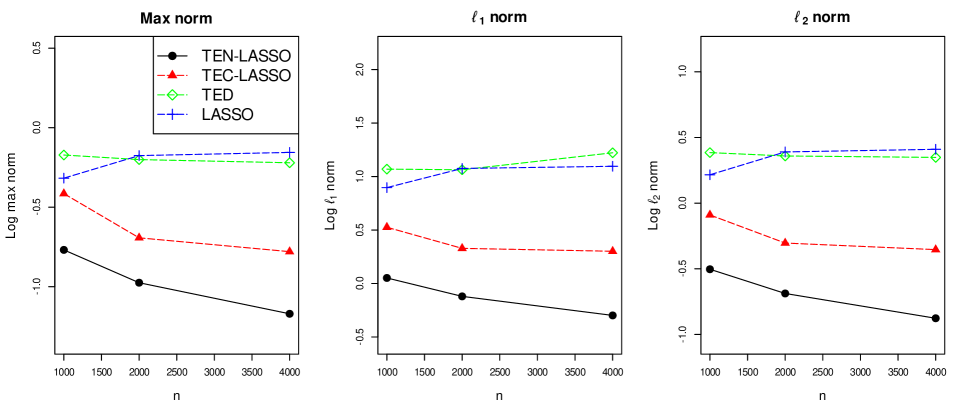
Figure 2: The log max, $\ell_{1}$, and $\ell_{2}$ norm error plots of the TEN-LASSO (black dot), TEC-LASSO (red triangle), TED (green diamond), and LASSO (blue plus) estimators for $p=100$ and $n=1000,2000,4000$.

Figure 2 plots the log max, $\ell_{1}$, and $\ell_{2}$ norm errors of the TEN-LASSO, TEC-LASSO, TED, and LASSO estimators with $n=1000,2000,4000$. As seen in Figure 2, the estimation errors of the TEN-LASSO estimator are decreasing as the sample size $n$ increases. As expected, the TEN-LASSO estimator outperforms other estimators for all error norms. This may be because only the TEN-LASSO estimator can fully explain the microstructure noise of high-frequency data and time-variation in the coefficient process. We note that the TED and LASSO estimators are not consistent. One possible explanation for this is that the proportion of the noise in log-returns increases as the sample size $n$ increases. These results indicate that the proposed TEN-LASSO estimator can help deal with the noises and time-varying coefficient process when estimating high-dimensional integrated coefficients.

5 An empirical study

We applied the proposed TEN-LASSO estimator to real high-frequency trading data, collected from January 2013 to December 2019. We obtained stock price data from the End of Day website (https://eoddata.com/), futures price data from the FirstRate Data website (https://firstratedata
.com/), and firm fundamentals from the Center for Research in Security Prices (CRSP)/Compustat Merged Database. We collected 1-min log-price data using the previous tick scheme (Wang and Zou,, 2010; Zhang,, 2011) and excluded the half trading days. For the dependent process, we considered the following five assets: Apple Inc. (AAPL), Berkshire Hathaway Inc. (BRK.B), General Motors Company (GM), Alphabet Inc. (GOOG), and Exxon Mobil Corporation (XOM). These assets have the largest market value in the following global industrial classification standards (GICS) sectors: information technology, financials, consumer discretionary, communication services, and energy. For the covariate process, we obtained the data of 54 futures, which are often considered as market macro variables. We chose 20 commodity futures, 10 currency futures, 10 interest rate futures, and 14 stock market index futures. Their symbols are listed in Table 3 in the Appendix. Furthermore, we constructed Fama-French five factors (Fama and French,, 2015) and the momentum factor (Carhart,, 1997) using high-frequency data. The MKT, HML, SMB, RMW, CMA, and MOM denote the market, value, size, profitability, investment, and momentum factors, respectively. For each of the six factors, we first obtained the monthly portfolio constituents among the stocks traded on NYSE, NASDAQ, and AMEX. Specifically, we obtained MKT as the return of a value-weighted portfolio of all assets, and the other factors were calculated as follows:

$$HML=\left(SH+BH\right)/2-\left(SL+BL\right)/2,$$

$$SMB=\left(SH+SM+SL\right)/3-\left(BH+BM+BL\right)/3,$$

$$RMW=\left(SR+BR\right)/2-\left(SW+BW\right)/2,$$

$$CMA=\left(SC+BC\right)/2-\left(SA+BA\right)/2,$$

$$MOM=\left(SU+BU\right)/2-\left(SD+BD\right)/2,$$

where small (S) and big (B) portfolios consist of assets with small and big market equities respectively, and we classified high (H), medium (M), and low (L) portfolios based on the ratio of book equity to market equity. In addition, robust (R), neutral (N), and weak (W) portfolios were classified by profitability, and we obtained the constituents of conservative (C), neutral (N), and aggressive (A) portfolios using the investment data. Finally, up (U), flat (F), and down (D) portfolios were classified by the momentum of the return. The details of this process can be found in Aït-Sahalia et al., (2020); Kim and Shin, (2022). Then, using 1-min high-frequency data, we calculated the portfolio returns as follows:

$$WRet_{d,i}=\dfrac{\sum_{s=1}^{N_{d}}w_{d,i}^{s}\times Ret_{d,i}^{s}}{\sum_{s=1}^{N_{d}}w_{d,i}^{s}},$$

where $WRet_{d,i}$ represents the portfolio return for the $d$th day and $i$th time interval, $N_{d}$ is the number of assets in the portfolio for the $d$th day (superscript $s$ represents the $s$th asset of the portfolio), and $w_{d,i}^{s}$ is defined by

$$w_{d,i}^{s}=w_{d}^{s}\times\prod_{l=0}^{i-1}\left(1+Ret_{d,l}^{s}\right),$$

where $w_{d}^{s}$ represents the market capitalization obtained using the close price of the $s$th stock on the $(d-1)$th day, and $Ret_{d,0}^{s}$ denotes the overnight return from the $\left(d-1\right)$th day to the $d$th day. To sum up, we used the five assets and 60 factors for the dependent and covariate processes, respectively.

When calculating the TEN-LASSO estimator, we employed the tuning parameter choice procedure discussed in Section 3.4 and Section 4. Moreover, we chose $k_{2}=390$, that is, we estimated instantaneous coefficients on a daily basis. To select the tuning parameter $c_{h}$, we utilized the mean squared prediction error (MSPE) using the data in $2013$. We first defined

$$\Lambda(c_{h})=\frac{1}{55}\sum_{m=1}^{11}\sum_{s=1}^{5}\left\|\widetilde{I\beta}^{m,s}\left(c_{h}\right)-\widehat{I\beta}^{(m+1),s}\right\|_{2}^{2},$$

where $\widetilde{I\beta}^{m,s}\left(c_{h}\right)$ is the TEN-LASSO estimator obtained with the tuning parameter $c_{h}$, and $\widehat{I\beta}^{m,s}$ is the debiased integrated coefficient estimator from the $m$th month in $2013$ and the $s$th stock. Then, we chose $c_{h}$ by minimizing $\Lambda(c_{h})$ over $c_{h}\in\left\{l/100\mid 0\leq l\leq 5,\,l\in\mathbb{Z}\right\}$. The result is $c_{h}=0.04$. We note that the stationarity condition on the coefficient process is reasonable, which motivates the above tuning parameter choice procedure. Then, we obtained the monthly integrated coefficients based on the TEN-LASSO, TEC-LASSO, TED, and LASSO estimation procedures for each of the five assets. The coefficients of the non-trading period were set as zero.

Table 1: Annual average in-sample and out-of-sample $R^{2}$ for the TEN-LASSO, TEC-LASSO, TED, and LASSO estimators over the five assets.

		In-sample $R^{2}$
		Estimator
		TEN-LASSO		TEC-LASSO		TED		LASSO
whole period		0.257		0.253		0.156		0.232
2013		0.225		0.230		0.101		0.199
2014		0.215		0.218		0.134		0.197
2015		0.275		0.272		0.176		0.246
2016		0.268		0.269		0.078		0.228
2017		0.230		0.228		0.176		0.169
2018		0.322		0.311		0.267		0.327
2019		0.263		0.245		0.162		0.259
		Out-of-sample $R^{2}$
		Estimator
		TEN-LASSO		TEC-LASSO		TED		LASSO
whole period		0.251		0.241		0.149		0.229
2014		0.189		0.180		0.099		0.178
2015		0.253		0.254		0.158		0.233
2016		0.258		0.249		0.058		0.226
2017		0.225		0.217		0.175		0.162
2018		0.332		0.323		0.245		0.321
2019		0.246		0.226		0.156		0.252

We first compared the performances of the TEN-LASSO, TEC-LASSO, TED, and LASSO estimators based on the monthly in-sample and out-of-sample $R^{2}$. The out-of-sample $R^{2}$ was obtained using the integrated coefficients from the previous month. For the out-of-sample $R^{2}$, we excluded the year $2013$, since we chose the tuning parameters using the data from $2013$. Then, we obtained the annual average $R^{2}$ across the five assets. Table 1 reports the annual average in-sample and out-of-sample $R^{2}$ for the TEN-LASSO, TEC-LASSO, TED, and LASSO estimators. From Table 1, we can see that the TEN-LASSO estimator shows the best performance overall. This may be because the proportion of the microstructure noise in 1-min high-frequency data is not negligible, and only the TEN-LASSO estimator can fully handle the noises and time-varying coefficient processes.

Table 2: Monthly average of the non-zero frequency of the TEN-LASSO, TEC-LASSO, TED, and LASSO estimators over 60 factors and 84 months for the five assets.

		Non-zero frequency
		Estimator
		TEN-LASSO		TEC-LASSO		TED		LASSO
AAPL		3.619		7.178		17.845		29.119
BRK.B		5.488		8.761		23.357		35.523
GM		4.428		8.071		25.750		30.642
GOOG		4.130		7.297		22.535		29.202
XOM		6.071		9.690		21.607		35.547

Table 2 reports the monthly average of non-zero frequency of the TEN-LASSO, TEC-LASSO, TED, and LASSO estimators over 60 factors and 84 months for the five assets. As seen in Table 2, the TEN-LASSO estimator is more sparse than the other estimators. Combining the results in Tables 1 and 2, we can conjecture that the proposed TEN-LASSO estimator can better account for market dynamics with a simpler model.

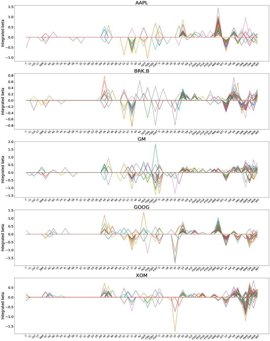
Figure 3: Monthly integrated coefficient estimates from the TEN-LASSO procedure for the five assets and 60 factors. Each line indicates the 60 integrated coefficient estimates from each month.

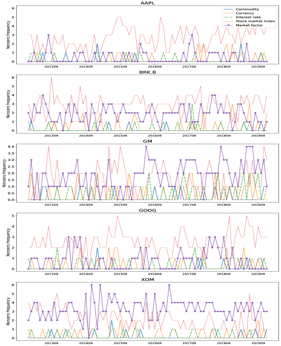
Figure 4: Nonzero frequency of the monthly integrated coefficient estimates from the TEN-LASSO procedure for the five assets and five groups, which consist of the commodity futures group, currency futures group, interest rate futures group, stock market index futures group, and market factor group.

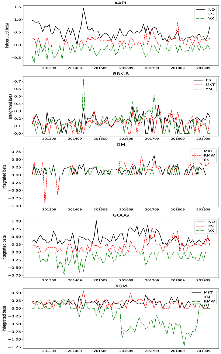
Figure 5: Monthly integrated coefficient estimates from the TEN-LASSO procedure for the three most frequent factors among the 60 factors for the five assets.

Now, we explore the integrated coefficient estimates from the TEN-LASSO procedure. Figure 3 plots the monthly integrated coefficients from the TEN-LASSO estimator for the five assets and 60 factors. Figure 4 shows the non-zero frequency of the TEN-LASSO estimator for the five groups, which consist of the commodity futures group, currency futures group, interest rate futures group, stock market index futures group, and market factor group. From Figures 3 and 4, we can see the time-variation and sparsity of the coefficient process. Furthermore, among the four futures groups, the stock market index futures group most frequently had non-zero integrated coefficients. This finding is in line with those of multi-factor models (Asness et al.,, 2013; Carhart,, 1997; Fama and French,, 1992, 2015), since the movements of stock market index futures factors can partially explain those of the market factors. To investigate the coefficient behaviors of the frequent factors, in Figure 5, we draw the integrated coefficient estimates for the three most frequent factors. AAPL has NQ (E-mini Nasdaq 100), ES (E-mini S&P 500), and VX (VIX); BRK.B has ES, MKT, and YM (E-mini Dow); GM has MKT, RMW, and ES; GOOG has NQ, ES, and VX; and XOM has MKT, YM, and RMW. We observed that all three factors belong to the stock market index futures group or the market factor group, which is also consistent with the results of multi-factor models.

6 Conclusion

In this paper, we developed a novel Thresholded dEbiased Nonconvex LASSO (TEN-LASSO) estimation procedure that can accommodate the microstructure noise of high-frequency data and time-variation in the high-dimensional coefficient process. When estimating the instantaneous coefficient, we employed the nonconvex optimization with the smoothed variables. We showed that the proposed instantaneous coefficient estimator can handle the noises and the high-dimensional time-varying coefficient process with the desirable convergence rate. To handle the bias from the $\ell_{1}$-regularization, we utilized the debiasing scheme and obtained the debiased integrated coefficient estimator using debiased instantaneous coefficient estimators. Then, we further regularized the debiased integrated coefficient estimator to account for the sparse structure of the coefficient process. We showed that the proposed TEN-LASSO estimator achieves the near-optimal convergence rate. In the empirical study, the TEN-LASSO estimation procedure performs best overall in terms of $R^{2}$. Furthermore, the TEN-LASSO estimator is more sparse compared with the other estimators. These findings suggest that when estimating high-dimensional integrated coefficients with high-frequency data, the proposed TEN-LASSO estimation method helps handle the time-varying property of the coefficient process as well as the microstructure noise in high-frequency data.

Appendix A Appendix

A.1 Proof of Theorem 1

Without loss of generality, it suffices to show the statement for fixed $i$. For simplicity, we denote the true instantaneous coefficient at time $i\Delta_{n}$ by $\boldsymbol{\beta}_{0}=(\beta_{10},\ldots,\beta_{p0})^{\top}$. Let

$$\mathcal{Y}^{c}_{i}=\begin{pmatrix}\sum^{k_{1}-1}_{l=0}g\left(\dfrac{l}{k_{1}}\right)\Delta_{i+l+1}^{n}Y^{c}\\ \sum^{k_{1}-1}_{l=0}g\left(\dfrac{l}{k_{1}}\right)\Delta_{i+l+2}^{n}Y^{c}\\ \vdots\\ \sum^{k_{1}-1}_{l=0}g\left(\dfrac{l}{k_{1}}\right)\Delta_{i+l+k_{2}-k_{1}+1}^{n}Y^{c}\end{pmatrix},\quad\mathcal{X}^{c}_{i}=\begin{pmatrix}\sum^{k_{1}-1}_{l=0}g\left(\dfrac{l}{k_{1}}\right)\Delta_{i+l+1}^{n}\mathbf{X}^{c\top}\\ \sum^{k_{1}-1}_{l=0}g\left(\dfrac{l}{k_{1}}\right)\Delta_{i+l+2}^{n}\mathbf{X}^{c\top}\\ \vdots\\ \sum^{k_{1}-1}_{l=0}g\left(\dfrac{l}{k_{1}}\right)\Delta_{i+l+k_{2}-k_{1}+1}^{n}\mathbf{X}^{c\top}\end{pmatrix},$$

$$\mathcal{Z}_{i}=\begin{pmatrix}\sum^{k_{1}-1}_{l=0}g\left(\dfrac{l}{k_{1}}\right)\Delta_{i+l+1}^{n}Z\\ \sum^{k_{1}-1}_{l=0}g\left(\dfrac{l}{k_{1}}\right)\Delta_{i+l+2}^{n}Z\\ \vdots\\ \sum^{k_{1}-1}_{l=0}g\left(\dfrac{l}{k_{1}}\right)\Delta_{i+l+k_{2}-k_{1}+1}^{n}Z\end{pmatrix},$$

$$\widetilde{\mathcal{X}}_{i}=\begin{pmatrix}\sum^{k_{1}-1}_{l=0}g\left(\dfrac{l}{k_{1}}\right)\int_{(i+l)\Delta_{n}}^{(i+l+1)\Delta_{n}}(\boldsymbol{\beta}(t)-\boldsymbol{\beta}_{0})^{\top}d\mathbf{X}^{c}(t)\\ \sum^{k_{1}-1}_{l=0}g\left(\dfrac{l}{k_{1}}\right)\int_{(i+l+1)\Delta_{n}}^{(i+l+2)\Delta_{n}}(\boldsymbol{\beta}(t)-\boldsymbol{\beta}_{0})^{\top}d\mathbf{X}^{c}(t)\\ \vdots\\ \sum^{k_{1}-1}_{l=0}g\left(\dfrac{l}{k_{1}}\right)\int_{(i+l+k_{2}-k_{1})\Delta_{n}}^{(i+l+k_{2}-k_{1}+1)\Delta_{n}}(\boldsymbol{\beta}(t)-\boldsymbol{\beta}_{0})^{\top}d\mathbf{X}^{c}(t)\end{pmatrix},$$

$$\mathcal{E}_{i}^{Y}=\begin{pmatrix}\sum^{k_{1}-1}_{l=0}g\left(\dfrac{l}{k_{1}}\right)\Delta_{i+l+1}^{n}\epsilon^{Y}\\ \sum^{k_{1}-1}_{l=0}g\left(\dfrac{l}{k_{1}}\right)\Delta_{i+l+2}^{n}\epsilon^{Y}\\ \vdots\\ \sum^{k_{1}-1}_{l=0}g\left(\dfrac{l}{k_{1}}\right)\Delta_{i+l+k_{2}-k_{1}+1}^{n}\epsilon^{Y}\end{pmatrix},\quad\mathcal{E}_{i}^{X}=\begin{pmatrix}\sum^{k_{1}-1}_{l=0}g\left(\dfrac{l}{k_{1}}\right)\Delta_{i+l+1}^{n}\left(\boldsymbol{\varepsilon}^{X}\right)^{\top}\\ \sum^{k_{1}-1}_{l=0}g\left(\dfrac{l}{k_{1}}\right)\Delta_{i+l+2}^{n}\left(\boldsymbol{\varepsilon}^{X}\right)^{\top}\\ \vdots\\ \sum^{k_{1}-1}_{l=0}g\left(\dfrac{l}{k_{1}}\right)\Delta_{i+l+k_{2}-k_{1}+1}^{n}\left(\boldsymbol{\varepsilon}^{X}\right)^{\top}\end{pmatrix}.$$

Then, we have

$$\mathcal{Y}^{c}_{i}=\mathcal{X}^{c}_{i}\boldsymbol{\beta}_{0}+\mathcal{Z}_{i}+\mathcal{\widetilde{X}}_{i}.$$

Also, let

$$\mathcal{Y}_{i}^{{}^{\prime}}=\begin{pmatrix}\sum^{k_{1}-1}_{l=0}g\left(\dfrac{l}{k_{1}}\right)\left\{\Delta_{i+l+1}^{n}Y^{c}+\Delta_{i+l+1}^{n}\epsilon^{Y}\right\}\,\boldsymbol{1}\left(|\Delta_{i}^{n}\widehat{Y}|\leq u_{n}\right)\\ \sum^{k_{1}-1}_{l=0}g\left(\dfrac{l}{k_{1}}\right)\left\{\Delta_{i+l+2}^{n}Y^{c}+\Delta_{i+l+2}^{n}\epsilon^{Y}\right\}\,\boldsymbol{1}\left(|\Delta_{i+1}^{n}\widehat{Y}|\leq u_{n}\right)\\ \vdots\\ \sum^{k_{1}-1}_{l=0}g\left(\dfrac{l}{k_{1}}\right)\left\{\Delta_{i+l+k_{2}-k_{1}+1}^{n}Y^{c}+\Delta_{i+l+k_{2}-k_{1}+1}^{n}\epsilon^{Y}\right\}\,\boldsymbol{1}\left(|\Delta_{i+k_{2}-k_{1}}^{n}\widehat{Y}|\leq u_{n}\right)\end{pmatrix}$$

and

$$\mathcal{X}_{i}^{{}^{\prime}}=\begin{pmatrix}\left(\Delta_{i}^{n}\widetilde{\mathbf{X}}^{\text{trunc}}\right)^{\top}\\ \left(\Delta_{i+1}^{n}\widetilde{\mathbf{X}}^{\text{trunc}}\right)^{\top}\\ \vdots\\ \left(\Delta_{i+k_{2}-k_{1}}^{n}\widetilde{\mathbf{X}}^{\text{trunc}}\right)^{\top}\end{pmatrix},$$

where

$$\Delta_{i}^{n}\widetilde{\mathbf{X}}^{\text{trunc}}=\left(\sum^{k_{1}-1}_{l=0}g\left(\dfrac{l}{k_{1}}\right)\left\{\Delta_{i+l+1}^{n}X^{c}_{j}+\Delta_{i+l+1}^{n}\epsilon^{X}_{j}\right\}\,\boldsymbol{1}\left(|\Delta_{i}^{n}\widehat{X}_{j}|\leq v_{j,n}\right)\right)_{j=1,\ldots,p}.$$

Proposition 2.

(Deviation condition) Under the assumptions in Theorem 1, we have, with the probability at least $1-p^{-1-a}$,

$$\left\|\nabla{\mathcal{L}}_{i}(\boldsymbol{\beta}_{0})\right\|_{\infty}\leq\eta/2.$$ (A.1)

Proof of Proposition 2. We have

$$\left\|\nabla{\mathcal{L}}_{i}(\boldsymbol{\beta}_{0})\right\|_{\infty} = \left\|\left(\dfrac{n}{\phi k_{1}k_{2}}\mathcal{X}_{i}^{\top}\mathcal{X}_{i}-\dfrac{n\zeta}{\phi k_{1}}\widehat{\mathbf{V}}^{X}\right)\boldsymbol{\beta}_{0}-\dfrac{n}{\phi k_{1}k_{2}}\mathcal{X}_{i}^{\top}\mathcal{Y}_{i}\right\|_{\infty}$$ (A.2)

$$\leq \left\|\left(\dfrac{n}{\phi k_{1}k_{2}}\mathcal{X}_{i}^{\top}\mathcal{X}_{i}-\dfrac{n\zeta}{\phi k_{1}}\widehat{\mathbf{V}}^{X}-\boldsymbol{\Sigma}_{0}(i\Delta_{n})\right)\boldsymbol{\beta}_{0}\right\|_{\infty}$$ (A.4)

$$+\left\|\dfrac{n}{\phi k_{1}k_{2}}\mathcal{X}_{i}^{\top}\mathcal{Y}_{i}-\boldsymbol{\Sigma}_{0}(i\Delta_{n})\boldsymbol{\beta}_{0}\right\|_{\infty}$$

$$= (I)+(II).$$ (A.5)

For $(I)$, we have

$$(I) \leq \left\|\left(\dfrac{n}{\phi k_{1}k_{2}}\mathcal{X}_{i}^{\top}\mathcal{X}_{i}-\dfrac{n\zeta}{\phi k_{1}}\mathbf{V}^{X}-\boldsymbol{\Sigma}_{0}(i\Delta_{n})\right)\boldsymbol{\beta}_{0}\right\|_{\infty}+\left\|\dfrac{n\zeta}{\phi k_{1}}\left(\widehat{\mathbf{V}}^{X}-\mathbf{V}^{X}\right)\boldsymbol{\beta}_{0}\right\|_{\infty}$$ (A.6)

$$= (I)^{(1)}+(I)^{(2)}.$$ (A.7)

Consider $(I)^{(1)}$. We have

$$\left\|\dfrac{n}{\phi k_{1}k_{2}}\mathcal{X}_{i}^{\top}\mathcal{X}_{i}-\dfrac{n\zeta}{\phi k_{1}}\mathbf{V}^{X}-\boldsymbol{\Sigma}_{0}(i\Delta_{n})\right\|_{\max}$$

$$\leq\dfrac{n}{\phi k_{1}k_{2}}\left\|\mathcal{X}_{i}^{\top}\mathcal{X}_{i}-\mathcal{X}_{i}^{{}^{\prime}\top}\mathcal{X}_{i}^{{}^{\prime}}\right\|_{\max}+\dfrac{n}{\phi k_{1}k_{2}}\left\|\mathcal{X}_{i}^{{}^{\prime}\top}\mathcal{X}_{i}^{{}^{\prime}}-\left(\mathcal{X}_{i}^{c}+\mathcal{E}_{i}^{X}\right)^{\top}\left(\mathcal{X}_{i}^{c}+\mathcal{E}_{i}^{X}\right)\right\|_{\max}$$

$$\quad+\left\|\dfrac{n}{\phi k_{1}k_{2}}\left(\mathcal{X}_{i}^{c}+\mathcal{E}_{i}^{X}\right)^{\top}\left(\mathcal{X}_{i}^{c}+\mathcal{E}_{i}^{X}\right)-\dfrac{n\zeta}{\phi k_{1}}\mathbf{V}^{X}-\boldsymbol{\Sigma}_{0}(i\Delta_{n})\right\|_{\max}$$

$$=(A)+(B)+(C).$$

For some large constant $C>0$, define

$$Q_{1} = \left\{\max_{i}\left\|\mathcal{X}_{i}^{c}\right\|_{\max}\leq C\sqrt{\dfrac{k_{1}\log p}{n}}\right\}\cap\left\{\max_{i}\left\|\mathcal{E}_{i}^{X}\right\|_{\max}\leq C\sqrt{\dfrac{\log p}{k_{1}}}\right\},$$

$$Q_{2} = \left\{\max_{i}\left\|\mathcal{Y}_{i}^{c}\right\|_{\infty}\leq Cs_{p}\sqrt{\dfrac{k_{1}\log p}{n}}\right\}\cap\left\{\max_{i}\left\|\mathcal{E}_{i}^{Y}\right\|_{\infty}\leq C\sqrt{\dfrac{\log p}{k_{1}}}\right\},$$

$$Q_{3} = \left\{\max_{i}\int_{i\Delta_{n}}^{\left(i+k_{2}\right)\Delta_{n}}d\Lambda^{Y}(t)\leq C\log p\right\}\cap\left\{\max_{i,j}\int_{i\Delta_{n}}^{\left(i+k_{2}\right)\Delta_{n}}d\Lambda_{j}(t)\leq C\log p\right\},$$

$$Q_{4} = \left\{\max_{i}\sum_{k=1}^{k_{2}-k_{1}+1}\boldsymbol{1}\left(|\Delta_{i+k-1}^{n}\widehat{Y}|>u_{n}\right)\leq Ck_{1}\log p\right\}$$

$$\cap\left\{\max_{i,j}\sum_{k=1}^{k_{2}-k_{1}+1}\boldsymbol{1}\left(|\Delta_{i+k-1}^{n}\widehat{X}_{j}|>v_{j,n}\right)\leq Ck_{1}\log p\right\},$$

$$Q_{5} = \left\{\max_{i}\left\|\mathcal{\widetilde{X}}_{i}\right\|_{\infty}\leq Cs_{p}n^{-3/8}\log p\right\}.$$

From Assumption 1(a)–(b), we can show

$$\Pr\left(Q_{1}\cap Q_{2}\right)\geq 1-p^{-2-a}.$$

By the boundedness of the intensity process, we have

$$\Pr\left(Q_{3}\right)\geq 1-p^{-2-a}.$$

Under $Q_{1}\cap Q_{2}\cap Q_{3}$, we have, for large $n$,

$$\max_{i}\sum_{k=1}^{k_{2}-k_{1}+1}\boldsymbol{1}\left(|\Delta_{i+k-1}^{n}\widehat{Y}|>u_{n}\right)\leq Ck_{1}\log p\quad\text{and}$$

$$\max_{i,j}\sum_{k=1}^{k_{2}-k_{1}+1}\boldsymbol{1}\left(|\Delta_{i+k-1}^{n}\widehat{X}_{j}|>v_{j,n}\right)\leq Ck_{1}\log p.$$

Consider $Q_{5}$. By Assumption 1(a), the process $\sum_{j=1}^{p}\left|\beta_{j}(t)-\beta_{j0}\right|$ has the sub-Gaussian tail. Then, similar to the proofs of Theorem 1 (Kim and Shin,, 2022), we can show

$$\Pr\left(Q_{5}\right)\geq 1-p^{-2-a}.$$

Thus, we have

$$\Pr\left(Q_{1}\cap Q_{2}\cap Q_{3}\cap Q_{4}\cap Q_{5}\right)\geq 1-3p^{-2-a}.$$ (A.8)

From (A.8), we have, with the probability at least $1-3p^{-2-a}$,

$$(A)\leq Cn^{-1/4}\left(\log p\right)^{2}\quad\text{ and }\quad(B)\leq Cn^{-1/4}\left(\log p\right)^{2}.$$

Also, similar to the proofs of Theorem 1 (Kim and Wang,, 2016), we can show

$$\Pr\left\{(C)\leq Cn^{-1/8}\sqrt{\log p}\right\}\geq 1-p^{-2-a},$$

which implies

$$\Pr\left\{\left\|\dfrac{n}{\phi k_{1}k_{2}}\mathcal{X}_{i}^{\top}\mathcal{X}_{i}-\dfrac{n\zeta}{\phi k_{1}}\mathbf{V}^{X}-\boldsymbol{\Sigma}_{0}(i\Delta_{n})\right\|_{\max}\leq C\left(n^{-1/4}\left(\log p\right)^{2}+n^{-1/8}\sqrt{\log p}\right)\right\}\geq 1-4p^{-2-a}$$

and

$$\Pr\left\{(I)^{(1)}\leq Cs_{p}\left(n^{-1/4}\left(\log p\right)^{2}+n^{-1/8}\sqrt{\log p}\right)\right\}\geq 1-4p^{-2-a}.$$ (A.9)

Similarly, we can show

$$\Pr\left\{(I)^{(2)}\leq Cs_{p}n^{-1/2}\sqrt{\log p}\right\}\geq 1-p^{-2-a}.$$ (A.10)

From (A.6),(A.9), and (A.10), we have

$$\Pr\left\{(I)\leq Cs_{p}\left(n^{-1/4}\left(\log p\right)^{2}+n^{-1/8}\sqrt{\log p}\right)\right\}\geq 1-5p^{-2-a}.$$ (A.11)

For $(II)$, we have

$$(II) \leq \dfrac{n}{\phi k_{1}k_{2}}\left\|\mathcal{X}_{i}^{\top}\mathcal{Y}_{i}-\left(\mathcal{X}_{i}^{c}+\mathcal{E}_{i}^{X}\right)^{\top}\left(\mathcal{Y}_{i}^{c}+\mathcal{E}_{i}^{Y}\right)\right\|_{\infty}+\left\|\left\{\dfrac{n}{\phi k_{1}k_{2}}\mathcal{X}_{i}^{c\top}\mathcal{X}_{i}^{c}-\boldsymbol{\Sigma}_{0}(i\Delta_{n})\right\}\boldsymbol{\beta}_{0}\right\|_{\infty}$$ (A.13)

$$+\dfrac{n}{\phi k_{1}k_{2}}\left\|\left(\mathcal{X}_{i}^{c}+\mathcal{E}_{i}^{X}\right)^{\top}\mathcal{\widetilde{X}}_{i}\right\|_{\infty}+\dfrac{n}{\phi k_{1}k_{2}}\left\|\mathcal{X}_{i}^{c\top}\left(\mathcal{Z}_{i}+\mathcal{E}_{i}^{Y}\right)+\left(\mathcal{E}_{i}^{X}\right)^{\top}\left(\mathcal{X}_{i}^{c}\boldsymbol{\beta}_{0}+\mathcal{Z}_{i}+\mathcal{E}_{i}^{Y}\right)\right\|_{\infty}$$

$$= (II)^{(1)}+(II)^{(2)}+(II)^{(3)}+(II)^{(4)}.$$ (A.14)

For $(II)^{(1)}$, note that

$$(II)^{(1)} \leq \dfrac{n}{\phi k_{1}k_{2}}\left\|\left(\mathcal{X}_{i}-\mathcal{X}_{i}^{{}^{\prime}}\right)^{\top}\mathcal{Y}_{i}\right\|_{\infty}+\dfrac{n}{\phi k_{1}k_{2}}\left\|\left(\mathcal{X}_{i}^{{}^{\prime}}-\mathcal{X}_{i}^{c}-\mathcal{E}_{i}^{X}\right)^{\top}\mathcal{Y}_{i}\right\|_{\infty}$$

$$+\dfrac{n}{\phi k_{1}k_{2}}\left\|\left(\mathcal{X}_{i}^{c}+\mathcal{E}_{i}^{X}\right)^{\top}\left(\mathcal{Y}_{i}-\mathcal{Y}_{i}^{{}^{\prime}}\right)\right\|_{\infty}+\dfrac{n}{\phi k_{1}k_{2}}\left\|\left(\mathcal{X}_{i}^{c}+\mathcal{E}_{i}^{X}\right)^{\top}\left(\mathcal{Y}_{i}^{{}^{\prime}}-\mathcal{Y}_{i}^{c}-\mathcal{E}_{i}^{Y}\right)\right\|_{\infty}.$$

Hence, by (A.8), we have

$$\Pr\left\{(II)^{(1)}\leq Cs_{p}n^{-1/4}\left(\log p\right)^{2}\right\}\geq 1-3p^{-2-a}.$$ (A.15)

For $(II)^{(2)}$, similar to the proofs of Theorem 1 (Kim and Wang,, 2016), we can show

$$\Pr\left((II)^{(2)}\leq Cs_{p}n^{-1/8}\sqrt{\log p}\right)\geq 1-p^{-2-a}.$$ (A.16)

Also, by (A.8), we have

$$\Pr\left((II)^{(3)}\leq Cs_{p}n^{-1/8}\left(\log p\right)^{3/2}\right)\geq 1-3p^{-2-a}.$$ (A.17)

For $(II)^{(4)}$, note that the elements of $\mathcal{X}_{i}^{c}$, $\mathcal{Z}_{i}$, $\mathcal{E}_{i}^{Y}$, and $\mathcal{E}_{i}^{X}$ have sub-Gaussian tails. Hence, by Bernstein’s inequality for martingales, we have

$$\Pr\left((II)^{(4)}\leq Cs_{p}n^{-1/8}\sqrt{\log p}\right)\geq 1-p^{-2-a}.$$ (A.18)

Combining (A.13)–(A.18), we have

$$\Pr\left((II)\leq Cs_{p}n^{-1/8}\left(\log p\right)^{3/2}\right)\geq 1-8p^{-2-a}.$$ (A.19)

Then, (A.1) is obtained by (A.2), (A.11), and (A.19). $\blacksquare$

Proposition 3.

(RE condition) Under the assumptions in Theorem 1, there exist positive constants $\alpha_{1}$, $\alpha_{2}$, and $\kappa$ such that, with the probability at least $1-p^{-1-a}$,

$$\boldsymbol{\beta}^{\top}\nabla^{2}{\mathcal{L}}_{i}(\boldsymbol{\beta})\boldsymbol{\beta}\geq\alpha_{1}\left\|\boldsymbol{\beta}\right\|_{2}^{2}-\kappa n^{-1/4}\log p\left\|\boldsymbol{\beta}\right\|_{1}^{2}\quad\text{ for all }\,\boldsymbol{\beta}\in\mathbb{R}^{p},$$ (A.20)

$$\boldsymbol{\beta}^{\top}\nabla^{2}{\mathcal{L}}_{i}(\boldsymbol{\beta})\boldsymbol{\beta}\leq\alpha_{2}\left\|\boldsymbol{\beta}\right\|_{2}^{2}+\kappa n^{-1/4}\log p\left\|\boldsymbol{\beta}\right\|_{1}^{2}\quad\text{ for all }\,\boldsymbol{\beta}\in\mathbb{R}^{p}.$$ (A.21)

Proof of Proposition 3. The drift term $\boldsymbol{\mu}(t)$ has a negligible order comparing with the Brownian motion term. Thus, for simplicity, we assume that $\boldsymbol{\mu}(t)=0$ for $0\leq t\leq 1$ without loss of generality. We have

$$\nabla^{2}{\mathcal{L}}_{i}(\boldsymbol{\beta})=\dfrac{n}{\phi k_{1}k_{2}}\mathcal{X}_{i}^{\top}\mathcal{X}_{i}-\dfrac{n\zeta}{\phi k_{1}}\widehat{\mathbf{V}}^{X}.$$ (A.22)

We first investigate $\dfrac{n}{\phi k_{1}k_{2}}\boldsymbol{\beta}^{\top}\mathcal{X}_{i}^{\top}\mathcal{X}_{i}\boldsymbol{\beta}$. By Assumption 1(c), for any unit vector $u\in\mathbb{R}^{p}$, the random variable $\left(\sqrt{n}u^{\top}\Delta_{i}^{n}\mathbf{X}^{c}\Big{|}\mathcal{F}_{(i-1)\Delta_{n}}\right)$ is sub-Gaussian with bounded parameter. Thus, each elment of $\left(\mathcal{X}_{i}^{c}+\mathcal{E}_{i}^{X}\right)\boldsymbol{\beta}$ has the sub-Gaussian tail with the order of $n^{-1/4}\left\|\boldsymbol{\beta}\right\|_{2}$. Then, using the Bernstein’s inequality for martingales, we can show, for any fixed unit vector $\boldsymbol{\beta}\in\mathbb{R}^{p}$,

$$\Pr\left\{\left|\boldsymbol{\beta}^{\top}\left(\dfrac{n}{\phi k_{1}k_{2}}\left(\mathcal{X}_{i}^{c}+\mathcal{E}_{i}^{X}\right)^{\top}\left(\mathcal{X}_{i}^{c}+\mathcal{E}_{i}^{X}\right)-\boldsymbol{\Sigma}_{0}(i\Delta_{n})-\dfrac{n\zeta}{\phi k_{1}}\mathbf{V}_{X}\right)\boldsymbol{\beta}\right|\leq\dfrac{\lambda_{\min}\left\{\boldsymbol{\Sigma}_{0}\left(i\Delta_{n}\right)\right\}}{432}\right\}$$ (A.24)

$$\geq 1-\exp\left(-c_{3}n^{1/4}\right)$$

for some constant $c_{3}>0$. For any parameter $s\geq 1$ and subset $U\subset\left\{1,\ldots,p\right\}$, define

$$\mathbb{K}\left(s\right)=\left\{\boldsymbol{\beta}\in\mathbb{R}^{p}\,\,\,|\,\,\,\|\boldsymbol{\beta}\|_{2}\leq 1,\,\|\boldsymbol{\beta}\|_{0}\leq s\right\}\quad\text{and}$$

$$A_{U}=\left\{\boldsymbol{\beta}\in\mathbb{R}^{p}\,\,\,|\,\,\,\|\boldsymbol{\beta}\|_{2}\leq 1,\,\operatorname{supp}\left(\boldsymbol{\beta}\right)\subset U\right\}.$$

By (A.24) and discretization argument in Lemma 15 (Loh and Wainwright,, 2012), we have, for any $A_{U}$ with $|U|\leq s$,

$$\Pr\left\{\left|\underset{\boldsymbol{\beta}\in A_{U}}{\sup}\,\boldsymbol{\beta}^{\top}\left(\dfrac{n}{\phi k_{1}k_{2}}\left(\mathcal{X}_{i}^{c}+\mathcal{E}_{i}^{X}\right)^{\top}\left(\mathcal{X}_{i}^{c}+\mathcal{E}_{i}^{X}\right)-\boldsymbol{\Sigma}_{0}(i\Delta_{n})-\dfrac{n\zeta}{\phi k_{1}}\mathbf{V}_{X}\right)\boldsymbol{\beta}\right|\leq\dfrac{\lambda_{\min}\left\{\boldsymbol{\Sigma}_{0}\left(i\Delta_{n}\right)\right\}}{432}\right\}$$

$$\geq 1-9^{s}\exp\left(-c_{3}n^{1/4}\right).$$

Note that $\mathbb{K}\left(s\right)=\cup_{|U|\leq s}A_{U}$ and $\binom{p}{s}\leq p^{s}$. Hence, we have, with the probability at least $1-\exp\left(-c_{3}n^{1/4}+s\log 9p\right)$,

$$\left|\underset{\boldsymbol{\beta}\in\mathbb{K}\left(s\right)}{\sup}\,\boldsymbol{\beta}^{\top}\left(\dfrac{n}{\phi k_{1}k_{2}}\left(\mathcal{X}_{i}^{c}+\mathcal{E}_{i}^{X}\right)^{\top}\left(\mathcal{X}_{i}^{c}+\mathcal{E}_{i}^{X}\right)-\boldsymbol{\Sigma}_{0}(i\Delta_{n})-\dfrac{n\zeta}{\phi k_{1}}\mathbf{V}_{X}\right)\boldsymbol{\beta}\right|\leq\dfrac{\lambda_{\min}\left\{\boldsymbol{\Sigma}_{0}\left(i\Delta_{n}\right)\right\}}{432}.$$

For some large constant $C>0$, let

$$A_{1}=\left\{\sum_{j=1}^{p}\int_{i\Delta_{n}}^{\left(i+k_{2}\right)\Delta_{n}}d\Lambda_{j}(t)\leq C\log p\right\},$$

$$A_{2}=\left\{\sum_{j=1}^{p}\sum_{k=1}^{k_{2}-k_{1}+1}\boldsymbol{1}\left(|\Delta_{i+k-1}^{n}\widehat{X}_{j}|>v_{j,n}\right)\leq Ck_{1}\log p\right\}.$$

By Assumption 1(c), similar to the proofs of (A.8), we can show

$$\Pr\left(Q_{1}\cap Q_{2}\cap A_{1}\cap A_{2}\right)\geq 1-p^{-2-a}.$$

Also, let $w_{k}$ be a $k$th row vector of $\mathcal{X}_{i}-\mathcal{X}_{i}^{c}-\mathcal{E}_{i}^{X}$. Under $Q_{1}$, we have

$$\underset{\left\|\boldsymbol{\beta}\right\|_{2}\leq 1}{\sup}\left|w_{k}\boldsymbol{\beta}\right|\leq C\max_{j}v_{j,n}\sqrt{\sum_{j=1}^{p}\boldsymbol{1}\left(|\Delta_{i+k-1}^{n}\widehat{X}_{j}|>v_{j,n}\right)}.$$

Thus, for large $n$, we have, with the probability at least $p^{-2-a}$,

$$\left|\underset{\boldsymbol{\beta}\in\mathbb{K}\left(s\right)}{\sup}\,\dfrac{n}{\phi k_{1}k_{2}}\boldsymbol{\beta}^{\top}\left(\mathcal{X}_{i}-\mathcal{X}_{i}^{c}-\mathcal{E}_{i}^{X}\right)^{\top}\left(\mathcal{X}_{i}-\mathcal{X}_{i}^{c}-\mathcal{E}_{i}^{X}\right)\boldsymbol{\beta}\right| \leq C\left(\max_{j}v_{j,n}\right)^{2}n^{1/4}\log p$$

$$\leq \dfrac{\lambda_{\min}\left\{\boldsymbol{\Sigma}_{0}\left(i\Delta_{n}\right)\right\}}{432}.$$

Then, by the Hölder’s inequality, we have, with the probability at least $1-\exp\left(-c_{3}n^{1/4}+s\log 9p\right)-p^{-2-a}$,

$$\left|\underset{\boldsymbol{\beta}\in\mathbb{K}\left(s\right)}{\sup}\,\boldsymbol{\beta}^{\top}\left(\dfrac{n}{\phi k_{1}k_{2}}\mathcal{X}_{i}^{\top}\mathcal{X}_{i}-\boldsymbol{\Sigma}_{0}(i\Delta_{n})-\dfrac{n\zeta}{\phi k_{1}}\mathbf{V}_{X}\right)\boldsymbol{\beta}\right|\leq\dfrac{\lambda_{\min}\left\{\boldsymbol{\Sigma}_{0}\left(i\Delta_{n}\right)\right\}}{108}.$$

Similarly, for some constant $c_{4}>0$, we can show

$$\Pr\left\{\left|\underset{\boldsymbol{\beta}\in\mathbb{K}\left(s\right)}{\sup}\,\boldsymbol{\beta}^{\top}\left(\dfrac{n\zeta}{\phi k_{1}}\widehat{\mathbf{V}}^{X}-\dfrac{n\zeta}{\phi k_{1}}\mathbf{V}_{X}\right)\boldsymbol{\beta}\right|\leq\dfrac{\lambda_{\min}\left\{\boldsymbol{\Sigma}_{0}\left(i\Delta_{n}\right)\right\}}{108}\right\}\geq 1-\exp\left(-c_{4}n+s\log 9p\right)-p^{-2-a},$$

which implies

$$\Pr\left\{\left|\underset{\boldsymbol{\beta}\in\mathbb{K}\left(s\right)}{\sup}\,\boldsymbol{\beta}^{\top}\left(\nabla^{2}{\mathcal{L}}_{i}(\boldsymbol{\beta})-\boldsymbol{\Sigma}_{0}(i\Delta_{n})\right)\boldsymbol{\beta}\right|\leq\dfrac{\lambda_{\min}\left\{\boldsymbol{\Sigma}_{0}\left(i\Delta_{n}\right)\right\}}{54}\right\}$$

$$\geq 1-2\exp\left(-c_{3}n^{1/4}+s\log 9p\right)-2p^{-2-a}$$

for large $n$. Then, by Lemma 13 (Loh and Wainwright,, 2012), we have, with the probability at least $1-2\exp\left(-c_{3}n^{1/4}+s\log 9p\right)-2p^{-2-a}$,

$$\boldsymbol{\beta}^{\top}\nabla^{2}{\mathcal{L}}_{i}(\boldsymbol{\beta})\boldsymbol{\beta}\geq\dfrac{\lambda_{\min}\left\{\boldsymbol{\Sigma}_{0}\left(i\Delta_{n}\right)\right\}}{2}\left\|\boldsymbol{\beta}\right\|_{2}^{2}-\dfrac{\lambda_{\min}\left\{\boldsymbol{\Sigma}_{0}\left(i\Delta_{n}\right)\right\}}{s}\left\|\boldsymbol{\beta}\right\|_{1}^{2}\quad\text{ for all }\,\boldsymbol{\beta}\in\mathbb{R}^{p},$$ (A.25)

$$\boldsymbol{\beta}^{\top}\nabla^{2}{\mathcal{L}}_{i}(\boldsymbol{\beta})\boldsymbol{\beta}\leq\dfrac{3\lambda_{\max}\left\{\boldsymbol{\Sigma}_{0}\left(i\Delta_{n}\right)\right\}}{2}\left\|\boldsymbol{\beta}\right\|_{2}^{2}+\dfrac{\lambda_{\min}\left\{\boldsymbol{\Sigma}_{0}\left(i\Delta_{n}\right)\right\}}{s}\left\|\boldsymbol{\beta}\right\|_{1}^{2}\quad\text{ for all }\,\boldsymbol{\beta}\in\mathbb{R}^{p}.$$ (A.26)

Choose

$$s=\dfrac{c_{3}n^{1/4}}{4\log p}.$$

Note that $c_{3}n^{1/4}\geq(2a+6)\log p$ for large $n$. Hence, we have, for large $n$,

$$2\exp\left(-c_{3}n^{1/4}+s\log 9p\right)+2p^{-2-a}\leq\exp\left(\log p-c_{3}n^{1/4}+c_{3}n^{1/4}/2\right)+2p^{-2-a}\leq p^{-1-a},$$

which completes the proof. $\blacksquare$

Proof of Theorem 1. By Propositions 2–3, it is enough to show the statement under (A.1), (A.20), and (A.21). From the optimality of $\widehat{\boldsymbol{\beta}}_{i\Delta_{n}}$, we can show

$$0 \geq {\mathcal{L}}_{i}(\widehat{\boldsymbol{\beta}}_{i\Delta_{n}})-{\mathcal{L}}_{i}(\boldsymbol{\beta}_{0})+\eta\left(\|\widehat{\boldsymbol{\beta}}_{i\Delta_{n}}\|_{1}-\left\|\boldsymbol{\beta}_{0}\right\|_{1}\right)$$

$$\geq \eta\left(\|\widehat{\boldsymbol{\beta}}_{i\Delta_{n}}\|_{1}-\left\|\boldsymbol{\beta}_{0}\right\|_{1}\right)+\langle\widehat{\boldsymbol{\beta}}_{i\Delta_{n}}-\boldsymbol{\beta}_{0},\nabla{\mathcal{L}}_{i}(\boldsymbol{\beta}_{0})\rangle+\frac{1}{2}\left(\widehat{\boldsymbol{\beta}}_{i\Delta_{n}}-\boldsymbol{\beta}_{0}\right)^{\top}\nabla^{2}{\mathcal{L}}_{i}(\boldsymbol{\beta})\left(\widehat{\boldsymbol{\beta}}_{i\Delta_{n}}-\boldsymbol{\beta}_{0}\right).$$

Note that

$$\|\widehat{\boldsymbol{\beta}}_{i\Delta_{n}}\|_{1}-\left\|\boldsymbol{\beta}_{0}\right\|_{1} \geq \left\|\left(\widehat{\boldsymbol{\beta}}_{i\Delta_{n}}\right)_{S}\right\|_{1}+\left\|\left(\widehat{\boldsymbol{\beta}}_{i\Delta_{n}}\right)_{S^{c}}\right\|_{1}$$

$$\geq \left\|\left(\widehat{\boldsymbol{\beta}}_{i\Delta_{n}}-\boldsymbol{\beta}_{0}\right)_{S^{c}}\right\|_{1}-\left\|\left(\widehat{\boldsymbol{\beta}}_{i\Delta_{n}}-\boldsymbol{\beta}_{0}\right)_{S}\right\|_{1}$$

and, by Proposition 2,

$$\langle\widehat{\boldsymbol{\beta}}_{i\Delta_{n}}-\boldsymbol{\beta}_{0},\nabla{\mathcal{L}}_{i}(\boldsymbol{\beta}_{0})\rangle\leq\left(\left\|\left(\widehat{\boldsymbol{\beta}}_{i\Delta_{n}}-\boldsymbol{\beta}_{0}\right)_{S}\right\|_{1}+\left\|\left(\widehat{\boldsymbol{\beta}}_{i\Delta_{n}}-\boldsymbol{\beta}_{0}\right)_{S^{c}}\right\|_{1}\right)\eta/2,$$

where $S$ is the support of $\boldsymbol{\beta}_{0}$. Hence, we have

$$\dfrac{3\eta}{2}\left\|\left(\widehat{\boldsymbol{\beta}}_{i\Delta_{n}}-\boldsymbol{\beta}_{0}\right)_{S}\right\|_{1}-\dfrac{\eta}{2}\left\|\left(\widehat{\boldsymbol{\beta}}_{i\Delta_{n}}-\boldsymbol{\beta}_{0}\right)_{S^{c}}\right\|_{1}$$ (A.27)

$$\geq\frac{1}{2}\left(\widehat{\boldsymbol{\beta}}_{i\Delta_{n}}-\boldsymbol{\beta}_{0}\right)^{\top}\nabla^{2}{\mathcal{L}}_{i}(\boldsymbol{\beta})\left(\widehat{\boldsymbol{\beta}}_{i\Delta_{n}}-\boldsymbol{\beta}_{0}\right)$$ (A.28)

$$\geq\dfrac{\alpha_{1}}{2}\left\|\widehat{\boldsymbol{\beta}}_{i\Delta_{n}}-\boldsymbol{\beta}_{0}\right\|_{2}^{2}-\dfrac{\kappa n^{-1/4}\log p}{2}\left\|\widehat{\boldsymbol{\beta}}_{i\Delta_{n}}-\boldsymbol{\beta}_{0}\right\|_{1}^{2},$$ (A.29)

where the last inequality is by Proposition 3. Also, using the fact that $\left\|\widehat{\boldsymbol{\beta}}_{i\Delta_{n}}-\boldsymbol{\beta}_{0}\right\|_{1}\leq Cs_{p}$, we have, for large $n$,

$$\eta\geq 2\kappa n^{-1/4}\log p\left\|\widehat{\boldsymbol{\beta}}_{i\Delta_{n}}-\boldsymbol{\beta}_{0}\right\|_{1}.$$

Therefore, by (A.27), we have

$$\left\|\left(\widehat{\boldsymbol{\beta}}_{i\Delta_{n}}-\boldsymbol{\beta}_{0}\right)_{S^{c}}\right\|_{1}\leq 7\left\|\left(\widehat{\boldsymbol{\beta}}_{i\Delta_{n}}-\boldsymbol{\beta}_{0}\right)_{S}\right\|_{1},$$

which implies

$$\left\|\widehat{\boldsymbol{\beta}}_{i\Delta_{n}}-\boldsymbol{\beta}_{0}\right\|_{1}\leq 8\sqrt{s_{p}}\left\|\widehat{\boldsymbol{\beta}}_{i\Delta_{n}}-\boldsymbol{\beta}_{0}\right\|_{2}.$$ (A.30)

Combining (A.27) and (A.30), we have, for large $n$,

$$12\sqrt{s_{p}}\eta\left\|\widehat{\boldsymbol{\beta}}_{i\Delta_{n}}-\boldsymbol{\beta}_{0}\right\|_{2} \geq \dfrac{3\eta}{2}\left\|\widehat{\boldsymbol{\beta}}_{i\Delta_{n}}-\boldsymbol{\beta}_{0}\right\|_{1}$$ (A.31)

$$\geq \dfrac{3\eta}{2}\left\|\left(\widehat{\boldsymbol{\beta}}_{i\Delta_{n}}-\boldsymbol{\beta}_{0}\right)_{S}\right\|_{1}-\dfrac{\eta}{2}\left\|\left(\widehat{\boldsymbol{\beta}}_{i\Delta_{n}}-\boldsymbol{\beta}_{0}\right)_{S^{c}}\right\|_{1}$$ (A.32)

$$\geq \dfrac{\alpha_{1}}{2}\left\|\widehat{\boldsymbol{\beta}}_{i\Delta_{n}}-\boldsymbol{\beta}_{0}\right\|_{2}^{2}-32\kappa s_{p}n^{-1/4}\log p\left\|\widehat{\boldsymbol{\beta}}_{i\Delta_{n}}-\boldsymbol{\beta}_{0}\right\|_{2}^{2}$$ (A.33)

$$\geq \dfrac{\alpha_{1}}{4}\left\|\widehat{\boldsymbol{\beta}}_{i\Delta_{n}}-\boldsymbol{\beta}_{0}\right\|_{2}^{2}.$$ (A.34)

Thus, we obtain

$$\left\|\widehat{\boldsymbol{\beta}}_{i\Delta_{n}}-\boldsymbol{\beta}_{0}\right\|_{2}\leq C\sqrt{s_{p}}\eta,$$ (A.35)

and then, by (A.30), we have

$$\left\|\widehat{\boldsymbol{\beta}}_{i\Delta_{n}}-\boldsymbol{\beta}_{0}\right\|_{1}\leq Cs_{p}\eta.$$ (A.36)

$\blacksquare$

A.2 Proof of Theorem 2

Proof of Theorem 2. To obtain the upper bound for $\|\widehat{I\beta}-I\beta_{0}\|_{\max}$, we first investigate $\widehat{\boldsymbol{\Omega}}_{i\Delta_{n}}$. We have

$$\sup_{0\leq i\leq n-k_{2}}\left\|\left(\dfrac{n}{\phi k_{1}k_{2}}\mathcal{X}_{i}^{\top}\mathcal{X}_{i}-\dfrac{n\zeta}{\phi k_{1}}\widehat{\mathbf{V}}^{X}\right)\boldsymbol{\Omega}_{0}\left(i\Delta_{n}\right)-\mathbf{I}\right\|_{\max}$$

$$\leq\sup_{0\leq i\leq n-k_{2}}\left\|\dfrac{n}{\phi k_{1}k_{2}}\mathcal{X}_{i}^{\top}\mathcal{X}_{i}-\dfrac{n\zeta}{\phi k_{1}}\widehat{\mathbf{V}}^{X}-\boldsymbol{\Sigma}_{0}\left(i\Delta_{n}\right)\right\|_{\max}\times\sup_{0\leq i\leq n-k_{2}}\left\|\boldsymbol{\Omega}_{0}\left(i\Delta_{n}\right)\right\|_{1}.$$

Similar to the proofs of (A.11), we can show

$$\Pr\left\{\sup_{0\leq i\leq n-k_{2}}\left\|\dfrac{n}{\phi k_{1}k_{2}}\mathcal{X}_{i}^{\top}\mathcal{X}_{i}-\dfrac{n\zeta}{\phi k_{1}}\widehat{\mathbf{V}}^{X}-\boldsymbol{\Sigma}_{0}\left(i\Delta_{n}\right)\right\|_{\max}\leq Cn^{-1/8}\sqrt{\log p}\right\}\geq 1-p^{-2-a}.$$

Thus, we have

$$\Pr\left\{\sup_{0\leq i\leq n-k_{2}}\|\widehat{\boldsymbol{\Omega}}_{i\Delta_{n}}\|_{1}\leq C\right\}\geq 1-p^{-2-a}.$$ (A.37)

Also, we have, with the probability at least $1-p^{-2-a}$,

$$\sup_{0\leq i\leq n-k_{2}}\left\|\boldsymbol{\Sigma}_{0}\left(i\Delta_{n}\right)\widehat{\boldsymbol{\Omega}}_{i\Delta_{n}}-\mathbf{I}\right\|_{\max} \leq \sup_{0\leq i\leq n-k_{2}}\left\|\left(\boldsymbol{\Sigma}_{0}\left(i\Delta_{n}\right)-\dfrac{n}{\phi k_{1}k_{2}}\mathcal{X}_{i}^{\top}\mathcal{X}_{i}+\dfrac{n\zeta}{\phi k_{1}}\widehat{\mathbf{V}}^{X}\right)\widehat{\boldsymbol{\Omega}}_{i\Delta_{n}}\right\|_{\max}$$

$$+\sup_{0\leq i\leq n-k_{2}}\left\|\left(\dfrac{n}{\phi k_{1}k_{2}}\mathcal{X}_{i}^{\top}\mathcal{X}_{i}-\dfrac{n\zeta}{\phi k_{1}}\widehat{\mathbf{V}}^{X}\right)\widehat{\boldsymbol{\Omega}}_{i\Delta_{n}}-\mathbf{I}\right\|_{\max}$$

$$\leq Cn^{-1/8}\sqrt{\log p},$$

which implies

$$\sup_{0\leq i\leq n-k_{2}}\|\widehat{\boldsymbol{\Omega}}_{i\Delta_{n}}-\boldsymbol{\Omega}_{0}\left(i\Delta_{n}\right)\|_{\max}$$

$$\leq\sup_{0\leq i\leq n-k_{2}}\|\boldsymbol{\Omega}_{0}\left(i\Delta_{n}\right)\|_{\infty}\times\sup_{0\leq i\leq n-k_{2}}\|\boldsymbol{\Sigma}_{0}\left(i\Delta_{n}\right)\widehat{\boldsymbol{\Omega}}_{i\Delta_{n}}-\mathbf{I}\|_{\max}$$

$$\leq Cn^{-1/8}\sqrt{\log p}.$$

Then, similar to the proofs of Theorem 1 (Kim and Shin,, 2022), we can show

$$\Pr\left\{\sup_{0\leq i\leq n-k_{2}}\|\widehat{\boldsymbol{\Omega}}_{i\Delta_{n}}-\boldsymbol{\Omega}_{0}\left(i\Delta_{n}\right)\|_{1}\leq Cs_{\omega,p}\left(n^{-1/8}\sqrt{\log p}\right)^{1-q}\right\}\geq 1-p^{-2-a}.$$ (A.38)

Let

$$\widetilde{\boldsymbol{\beta}}_{i\Delta_{n}}^{(2)}=\widehat{\boldsymbol{\beta}}_{i\Delta_{n}}+\dfrac{n}{\phi k_{1}k_{2}}\widehat{\boldsymbol{\Omega}}_{i\Delta_{n}}^{\top}\Big{[}\left(\mathcal{X}_{i}^{c}+\mathcal{E}_{i}^{X}\right)^{\top}\left(\mathcal{Y}_{i}^{c}+\mathcal{E}_{i}^{Y}\right)$$

$$\qquad\qquad\qquad\qquad\qquad\qquad-\left(\left(\mathcal{X}_{i}^{c}+\mathcal{E}_{i}^{X}\right)^{\top}\left(\mathcal{X}_{i}^{c}+\mathcal{E}_{i}^{X}\right)-k_{2}\zeta\widehat{\mathbf{V}}^{X}\right)\widehat{\boldsymbol{\beta}}_{i\Delta_{n}}\Big{]},$$

$$\widetilde{\boldsymbol{\beta}}_{i\Delta_{n}}^{(3)}=\boldsymbol{\beta}_{0}\left(i\Delta_{n}\right)+\dfrac{n}{\phi k_{1}k_{2}}\widehat{\boldsymbol{\Omega}}_{i\Delta_{n}}^{\top}\Big{[}\left(\mathcal{X}_{i}^{c}+\mathcal{E}_{i}^{X}\right)^{\top}\left(\mathcal{Z}_{i}+\mathcal{\widetilde{X}}_{i}+\mathcal{E}_{i}^{Y}\right)$$

$$\qquad\qquad\qquad\qquad\qquad\qquad\qquad-\left(\left(\mathcal{X}_{i}^{c}+\mathcal{E}_{i}^{X}\right)^{\top}\mathcal{E}_{i}^{X}-k_{2}\zeta\widehat{\mathbf{V}}^{X}\right)\widehat{\boldsymbol{\beta}}_{i\Delta_{n}}\Big{]},$$

$$\widetilde{\boldsymbol{\beta}}_{i\Delta_{n}}^{(4)}=\boldsymbol{\beta}_{0}\left(i\Delta_{n}\right)+\dfrac{n}{\phi k_{1}k_{2}}\boldsymbol{\Omega}_{0}\left(i\Delta_{n}\right)\Big{[}\left(\mathcal{X}_{i}^{c}+\mathcal{E}_{i}^{X}\right)^{\top}\left(\mathcal{Z}_{i}+\mathcal{\widetilde{X}}_{i}+\mathcal{E}_{i}^{Y}\right)$$

$$\qquad\qquad\qquad\qquad\qquad\qquad\qquad\qquad-\left(\left(\mathcal{X}_{i}^{c}+\mathcal{E}_{i}^{X}\right)^{\top}\mathcal{E}_{i}^{X}-k_{2}\zeta\mathbf{V}^{X}\right)\boldsymbol{\beta}_{0}\left(i\Delta_{n}\right)\Big{]}.$$

We have

$$\|\widehat{I\beta}-I\beta_{0}\|_{\max} \leq \left\|\sum_{i=0}^{[1/(k_{2}\Delta_{n})]-1}\left(\widetilde{\boldsymbol{\beta}}_{ik_{2}\Delta_{n}}-\widetilde{\boldsymbol{\beta}}_{ik_{2}\Delta_{n}}^{(2)}\right)k_{2}\Delta_{n}\right\|_{\infty}$$ (A.44)

$$+\left\|\sum_{i=0}^{[1/(k_{2}\Delta_{n})]-1}\left(\widetilde{\boldsymbol{\beta}}_{ik_{2}\Delta_{n}}^{(2)}-\widetilde{\boldsymbol{\beta}}_{ik_{2}\Delta_{n}}^{(3)}\right)k_{2}\Delta_{n}\right\|_{\infty}$$

$$+\left\|\sum_{i=0}^{[1/(k_{2}\Delta_{n})]-1}\left(\widetilde{\boldsymbol{\beta}}_{ik_{2}\Delta_{n}}^{(3)}-\widetilde{\boldsymbol{\beta}}_{ik_{2}\Delta_{n}}^{(4)}\right)k_{2}\Delta_{n}\right\|_{\infty}$$

$$+\left\|\sum_{i=0}^{[1/(k_{2}\Delta_{n})]-1}\left(\widetilde{\boldsymbol{\beta}}_{ik_{2}\Delta_{n}}^{(4)}-\boldsymbol{\beta}_{0}(ik_{2}\Delta_{n})\right)k_{2}\Delta_{n}\right\|_{\infty}$$

$$+\left\|\sum_{i=0}^{[1/(k_{2}\Delta_{n})]-1}\int_{ik_{2}\Delta_{n}}^{(i+1)k_{2}\Delta_{n}}\left(\boldsymbol{\beta}_{0}(ik_{2}\Delta_{n})-\boldsymbol{\beta}_{0}(t)\right)dt\right\|_{\infty}$$

$$+\left\|\int_{[1/(k_{2}\Delta_{n})]k_{2}\Delta_{n}}^{1}\boldsymbol{\beta}_{0}(t)dt\right\|_{\infty}$$

$$= (I)+(II)+(III)+(IV)+(V)+(VI).$$ (A.45)

Consider $(I)$. For some large constant $C>0$, define

$$B_{1}=\left\{\int_{0}^{1}d\Lambda^{Y}(t)\leq C\log p\right\}\cap\left\{\max_{j}\int_{0}^{1}d\Lambda_{j}(t)\leq C\log p\right\},$$

$$B_{2}=\left\{\sum_{i=0}^{n-k_{1}}\boldsymbol{1}\left(|\Delta_{i}^{n}\widehat{Y}|>u_{n}\right)\leq Ck_{1}\log p\right\}\cap\left\{\max_{j}\sum_{i=0}^{n-k_{1}}\boldsymbol{1}\left(|\Delta_{i}^{n}\widehat{X}_{j}|>v_{j,n}\right)\leq Ck_{1}\log p\right\}.$$

By the proofs of (A.8), we can show

$$\Pr\left(Q_{1}\cap Q_{2}\cap B_{1}\cap B_{2}\right)\geq 1-p^{-2-a}.$$ (A.46)

Then, by (3.9) and (A.37), we have

$$\Pr\left\{(I)\leq Cs_{p}n^{-1/4}(\log p)^{2}\right\}\geq 1-p^{-1-a}.$$ (A.47)

Consider $(II)$. Similar to the proofs of Theorem 1 (Kim and Wang,, 2016), we can show, with the probability at least $1-p^{-2-a}$,

$$\sup_{0\leq i\leq n-k_{2}}\left\|\dfrac{n}{\phi k_{1}k_{2}}\left(\mathcal{X}_{i}^{c}+\mathcal{E}_{i}^{X}\right)^{\top}\mathcal{X}_{i}^{c}-\boldsymbol{\Sigma}_{0}\left(i\Delta_{n}\right)\right\|_{\max}\leq Cn^{-1/8}\sqrt{\log p}\quad\text{and}$$

$$\sup_{0\leq i\leq n-k_{2}}\left\|\dfrac{n}{\phi k_{1}k_{2}}\left(\mathcal{X}_{i}^{c}+\mathcal{E}_{i}^{X}\right)^{\top}\left(\mathcal{X}_{i}^{c}+\mathcal{E}_{i}^{X}\right)-\dfrac{n\zeta}{\phi k_{1}}\widehat{\mathbf{V}}^{X}-\boldsymbol{\Sigma}_{0}\left(i\Delta_{n}\right)\right\|_{\max}\leq Cn^{-1/8}\sqrt{\log p}.$$

Thus, by (A.37) and (A.46), we have, with the probability at least $1-3p^{-2-a}$,

$$\sup_{0\leq i\leq n-k_{2}}\left\|\dfrac{n}{\phi k_{1}k_{2}}\widehat{\boldsymbol{\Omega}}_{i\Delta_{n}}^{\top}\left(\mathcal{X}_{i}^{c}+\mathcal{E}_{i}^{X}\right)^{\top}\mathcal{X}_{i}^{c}-\mathbf{I}\right\|_{\max}$$

$$\leq\sup_{0\leq i\leq n-k_{2}}\left\|\widehat{\boldsymbol{\Omega}}_{i\Delta_{n}}^{\top}\right\|_{\infty}\times\sup_{0\leq i\leq n-k_{2}}\left\|\dfrac{n}{\phi k_{1}k_{2}}\left(\mathcal{X}_{i}^{c}+\mathcal{E}_{i}^{X}\right)^{\top}\mathcal{X}_{i}^{c}-\boldsymbol{\Sigma}_{0}\left(i\Delta_{n}\right)\right\|_{\max}$$

$$\quad+\sup_{0\leq i\leq n-k_{2}}\left\|\widehat{\boldsymbol{\Omega}}_{i\Delta_{n}}^{\top}\right\|_{\infty}\times\sup_{0\leq i\leq n-k_{2}}\left\|\boldsymbol{\Sigma}_{0}\left(i\Delta_{n}\right)-\dfrac{n}{\phi k_{1}k_{2}}\left(\mathcal{X}_{i}^{c}+\mathcal{E}_{i}^{X}\right)^{\top}\left(\mathcal{X}_{i}^{c}+\mathcal{E}_{i}^{X}\right)+\dfrac{n\zeta}{\phi k_{1}}\widehat{\mathbf{V}}^{X}\right\|_{\max}$$

$$\quad+\sup_{0\leq i\leq n-k_{2}}\left\|\widehat{\boldsymbol{\Omega}}_{i\Delta_{n}}^{\top}\right\|_{\infty}\times\sup_{0\leq i\leq n-k_{2}}\left\|\dfrac{n}{\phi k_{1}k_{2}}\left(\left(\mathcal{X}_{i}^{c}+\mathcal{E}_{i}^{X}\right)^{\top}\left(\mathcal{X}_{i}^{c}+\mathcal{E}_{i}^{X}\right)-\mathcal{X}_{i}^{\top}\mathcal{X}_{i}\right)\right\|_{\max}$$

$$\quad+\sup_{0\leq i\leq n-k_{2}}\left\|\widehat{\boldsymbol{\Omega}}_{i\Delta_{n}}^{\top}\left(\dfrac{n}{\phi k_{1}k_{2}}\mathcal{X}_{i}^{\top}\mathcal{X}_{i}-\dfrac{n\zeta}{\phi k_{1}}\widehat{\mathbf{V}}^{X}\right)-\mathbf{I}\right\|_{\max}$$

$$\leq Cn^{-1/8}\sqrt{\log p}.$$

Then, from (3.9), we have, with the probability at least $1-p^{-1-a}$,

$$(II) \leq \sup_{0\leq i\leq n-k_{2}}\left\|\dfrac{n}{\phi k_{1}k_{2}}\widehat{\boldsymbol{\Omega}}_{i\Delta_{n}}^{\top}\left(\mathcal{X}_{i}^{c}+\mathcal{E}_{i}^{X}\right)^{\top}\mathcal{X}_{i}^{c}-\mathbf{I}\right\|_{\max}\times\sup_{0\leq i\leq n-k_{2}}\left\|\widehat{\boldsymbol{\beta}}_{i\Delta_{n}}-\boldsymbol{\beta}_{0}\left(i\Delta_{n}\right)\right\|_{1}$$ (A.48)

$$\leq Cs_{p}^{2}n^{-1/4}\left(\log p\right)^{2}.$$ (A.49)

For $(III)$, we have

$$(III) \leq \sup_{0\leq i\leq n-k_{2}}\left\|\widehat{\boldsymbol{\Omega}}_{i\Delta_{n}}^{\top}\right\|_{\infty}\times\sup_{0\leq i\leq n-k_{2}}\left\|\dfrac{n\zeta}{\phi k_{1}}\left(\widehat{\mathbf{V}}^{X}-\mathbf{V}^{X}\right)\right\|_{\max}\times\sup_{0\leq i\leq n-k_{2}}\left\|\widehat{\boldsymbol{\beta}}_{i\Delta_{n}}\right\|_{1}$$

$$+\sup_{0\leq i\leq n-k_{2}}\left\|\widehat{\boldsymbol{\Omega}}_{i\Delta_{n}}^{\top}-\boldsymbol{\Omega}_{0}\left(i\Delta_{n}\right)\right\|_{\infty}$$

$$\quad\times\sup_{0\leq i\leq n-k_{2}}\dfrac{n}{\phi k_{1}k_{2}}\left\|\left(\mathcal{X}_{i}^{c}+\mathcal{E}_{i}^{X}\right)^{\top}\left(\mathcal{Z}_{i}+\mathcal{E}_{i}^{Y}\right)-\left(\left(\mathcal{X}_{i}^{c}+\mathcal{E}_{i}^{X}\right)^{\top}\mathcal{E}_{i}^{X}-k_{2}\zeta\mathbf{V}^{X}\right)\widehat{\boldsymbol{\beta}}_{i\Delta_{n}}\right\|_{\max}$$

$$+\sup_{0\leq i\leq n-k_{2}}\left\|\widehat{\boldsymbol{\Omega}}_{i\Delta_{n}}^{\top}-\boldsymbol{\Omega}_{0}\left(i\Delta_{n}\right)\right\|_{\infty}\times\sup_{0\leq i\leq n-k_{2}}\dfrac{n}{\phi k_{1}k_{2}}\left\|\left(\mathcal{X}_{i}^{c}+\mathcal{E}_{i}^{X}\right)^{\top}\mathcal{\widetilde{X}}_{i}\right\|_{\max}$$

$$+\sup_{0\leq i\leq n-k_{2}}\left\|\boldsymbol{\Omega}_{0}\left(i\Delta_{n}\right)\right\|_{\infty}\times\sup_{0\leq i\leq n-k_{2}}\left\|\dfrac{n}{\phi k_{1}k_{2}}\left(\mathcal{X}_{i}^{c}+\mathcal{E}_{i}^{X}\right)^{\top}\mathcal{E}_{i}^{X}-\dfrac{n\zeta}{\phi k_{1}}\mathbf{V}^{X}\right\|_{\max}$$

$$\quad\times\sup_{0\leq i\leq n-k_{2}}\left\|\widehat{\boldsymbol{\beta}}_{i\Delta_{n}}-\boldsymbol{\beta}_{0}\left(i\Delta_{n}\right)\right\|_{1}.$$

Similar to the proofs of (A.11), we can show, with the probability at least $1-p^{-2-a}$,

$$\sup_{0\leq i\leq n-k_{2}}\left\|\dfrac{n\zeta}{\phi k_{1}}\left(\widehat{\mathbf{V}}^{X}-\mathbf{V}^{X}\right)\right\|_{\max}\leq Cn^{-1/2}\sqrt{\log p}.$$

By the Bernstein’s inequality for martingales, we have, with the probability at least $1-p^{-2-a}$,

$$\sup_{0\leq i\leq n-k_{2}}\dfrac{n}{\phi k_{1}k_{2}}\left\|\left(\mathcal{X}_{i}^{c}+\mathcal{E}_{i}^{X}\right)^{\top}\left(\mathcal{Z}_{i}+\mathcal{E}_{i}^{Y}\right)-\left(\left(\mathcal{X}_{i}^{c}+\mathcal{E}_{i}^{X}\right)^{\top}\mathcal{E}_{i}^{X}-k_{2}\zeta\mathbf{V}^{X}\right)\widehat{\boldsymbol{\beta}}_{i\Delta_{n}}\right\|_{\max}$$

$$\leq Cs_{p}n^{-1/8}\sqrt{\log p}\quad\text{and}$$

$$\sup_{0\leq i\leq n-k_{2}}\left\|\dfrac{n}{\phi k_{1}k_{2}}\left(\mathcal{X}_{i}^{c}+\mathcal{E}_{i}^{X}\right)^{\top}\mathcal{E}_{i}^{X}-\dfrac{n\zeta}{\phi k_{1}}\mathbf{V}^{X}\right\|_{\max}\leq Cn^{-1/8}\sqrt{\log p}.$$

Also, by (A.46), we have

$$\Pr\left(\sup_{0\leq i\leq n-k_{2}}\dfrac{n}{\phi k_{1}k_{2}}\left\|\left(\mathcal{X}_{i}^{c}+\mathcal{E}_{i}^{X}\right)^{\top}\mathcal{\widetilde{X}}_{i}\right\|_{\max}\leq Cs_{p}n^{-1/8}\left(\log p\right)^{3/2}\right)\geq 1-3p^{-2-a}.$$

Then, from (3.9), (A.37), and (A.38), we have

$$\Pr\left\{(III)\leq C\left[s_{p}s_{\omega,p}n^{\left(-2+q\right)/8}\left(\log p\right)^{\left(4-q\right)/2}+s_{p}^{2}n^{-1/4}\left(\log p\right)^{2}\right]\right\}\geq 1-p^{-1-a}.$$ (A.50)

Consider $(IV)$. We have

$$(IV) \leq C\Bigg{\|}\sum_{i=0}^{[1/(k_{2}\Delta_{n})]-1}\boldsymbol{\Omega}_{0}\left(ik_{2}\Delta_{n}\right)\Big{[}\left(\mathcal{X}_{ik_{2}}^{c}+\mathcal{E}_{ik_{2}}^{X}\right)^{\top}\left(\mathcal{Z}_{ik_{2}}+\mathcal{E}_{ik_{2}}^{Y}\right)$$

$$\qquad\qquad-\left(\left(\mathcal{X}_{ik_{2}}^{c}+\mathcal{E}_{ik_{2}}^{X}\right)^{\top}\mathcal{E}_{ik_{2}}^{X}-k_{2}\zeta\mathbf{V}^{X}\right)\boldsymbol{\beta}_{0}\left(ik_{2}\Delta_{n}\right)\Big{]}\Bigg{\|}_{\infty}$$

$$\quad+C\Bigg{\|}\sum_{i=0}^{[1/(k_{2}\Delta_{n})]-1}\boldsymbol{\Omega}_{0}\left(ik_{2}\Delta_{n}\right)\left(\mathcal{X}_{ik_{2}}^{c}+\mathcal{E}_{ik_{2}}^{X}\right)^{\top}\mathcal{\widetilde{X}}_{ik_{2}}\Bigg{\|}_{\infty}.$$

For the first term, note that each element of $\mathcal{X}_{i}^{c}$, $\mathcal{Z}_{i}$, $\mathcal{E}_{i}^{Y}$, and $\mathcal{E}_{i}^{X}$ has sub-Gaussian tail. Thus, using Bernstein’s inequality for martingales, we can show, with the probability at least $1-p^{-2-a}$,

$$\Bigg{\|}\sum_{i=0}^{[1/(k_{2}\Delta_{n})]-1}\boldsymbol{\Omega}_{0}\left(ik_{2}\Delta_{n}\right)\Big{[}\left(\mathcal{X}_{ik_{2}}^{c}+\mathcal{E}_{ik_{2}}^{X}\right)^{\top}\left(\mathcal{Z}_{ik_{2}}+\mathcal{E}_{ik_{2}}^{Y}\right)$$

$$\qquad\qquad-\left(\left(\mathcal{X}_{ik_{2}}^{c}+\mathcal{E}_{ik_{2}}^{X}\right)^{\top}\mathcal{E}_{ik_{2}}^{X}-k_{2}\zeta\mathbf{V}^{X}\right)\boldsymbol{\beta}_{0}\left(ik_{2}\Delta_{n}\right)\Big{]}\Bigg{\|}_{\infty}$$

$$\leq Cs_{p}n^{-1/4}\sqrt{\log p}.$$

For the second term, let

$$E=\left\{\sup_{0\leq i\leq n-k_{2}}\sup_{t\in[i\Delta_{n},\left(i+k_{2}\right)\Delta_{n}]}\sum_{j=1}^{p}\left|\beta_{j0}(t)-\beta_{j0}(i\Delta_{n})\right|\leq Cs_{p}n^{-1/8}\sqrt{\log p}\right\}.$$

Then, similar to the proofs of Theorem 1 (Kim and Shin,, 2022), we can show

$$\Pr\left(E\right)\geq 1-p^{-2-a}.$$

Under the event $E$, each element of $\left(\mathcal{X}_{i}^{c}+\mathcal{E}_{i}^{X}\right)^{\top}\mathcal{\widetilde{X}}_{i}$ has sub-exponential tail with the order of $s_{p}n^{-3/8}\sqrt{\log p}$. Thus, by Bernstein’s inequality for martingales, we can show, with the probability at least $1-2p^{-2-a}$,

$$\left\|\sum_{i=0}^{[1/(k_{2}\Delta_{n})]-1}\boldsymbol{\Omega}_{0}\left(ik_{2}\Delta_{n}\right)\left(\mathcal{X}_{ik_{2}}^{c}+\mathcal{E}_{ik_{2}}^{X}\right)^{\top}\mathcal{\widetilde{X}}_{ik_{2}}\right\|_{\infty}\leq Cs_{p}n^{-1/4}\log p,$$

which implies

$$\Pr\left\{(IV)\leq Cs_{p}n^{-1/4}\log p\right\}\geq 1-p^{-1-a}.$$ (A.51)

Consider $(V)$. Since the process $\boldsymbol{\beta}_{0}(t)$ has the sub-Gaussian tail, we can show

$$\Pr\left\{(V)\leq Cn^{-1/4}\sqrt{\log p}\right\}\geq 1-p^{-1-a}.$$ (A.52)

For $(VI)$, by Assumption 1(a), we have

$$(VI)\leq Cn^{-1/4}\text{ a.s.}$$ (A.53)

Combining (A.44) and (A.47)–(A.53), we have, with the probability at least $1-p^{-a}$,

$$\|\widehat{I\beta}-I\beta_{0}\|_{\max}\leq C\left\{s_{p}^{2}n^{-1/4}\left(\log p\right)^{2}+s_{p}s_{\omega,p}n^{\left(-2+q\right)/8}\left(\log p\right)^{\left(4-q\right)/2}\right\}.$$ (A.54)

$\blacksquare$

A.3 Proof of Theorem 3

Proof of Theorem 3. By (3.10), there exists a constant $C_{h}$ such that

$$\Pr\left\{\|\widehat{I\beta}-I\beta_{0}\|_{\max}\leq h_{n}/2\right\}\geq 1-p^{-a}.$$

Thus, it suffices to show the statement under $\{\|\widehat{I\beta}-I\beta_{0}\|_{\max}\leq h_{n}/2\}$. Similar to the proofs of Theorem 1 (Kim and Shin,, 2022), we can obtain

$$\|\widetilde{I\beta}-I\beta_{0}\|_{1}\leq Cs_{p}h_{n}.$$

$\blacksquare$

A.4 Proof of Proposition 1

Proof of Proposition 1. By Proposition 3, we can show Proposition 1 similar to the proofs of Theorem 2 (Agarwal et al.,, 2012). $\blacksquare$

Type		Symbol		Description
Commodity		C		Cocoa
		CL		Crude Oil WTI
		CSC		Cash-Settled Cheese
		CT		Cotton #2
		EBM		Milling Wheat
		GC		Gold
		HG		Copper
		NG		Henry Hub Natural Gas
		OJ		Orange Juice
		PA		Palladium
		PL		Platinum
		RM		Robusta Coffee
		SB		Sugar #11
		SI		Silver
		ZC		Corn
		ZL		Soybean Oil
		ZM		Soybean Meal
		ZO		Oats
		ZR		Rough Rice
		ZW		Wheat
Currency		A6		Australian Dollar
		AD		Canadian Dollar
		B6		British Pound
		BR		Brazilian Real
		DX		US Dollar Index
		E1		Swiss Franc
		E7		E-Mini Euro FX
		J1		Japanese Yen
		RP		Euro/British Pound
		RU		Russian Ruble
Interest rate		FBTP		Euro BTP Long-Bond
		FGBL		Euro Bund
		FGBX		Euro-Buxl
		FOAT		Euro-OAT
		G		10-Year Long Gilt
		TN		Ultra 10-Year Us Treasury Note
		UB		Ultra Us Treasury Bond
		US		30-Year US Treasury Bond
		ZF		5-Year US Treasury Note
		ZN		10-Year US Treasury Note
Stock market index		ES		E-mini S&P 500
		EW		E-mini S&P 400 Midcap
		FCE		CAC 40
		FDAX		DAX
		FESX		Euro Stoxx 50
		FTUK		FTSE 100
		FVSA		Vstoxx
		FXXP		Stoxx Europe 600 Index
		MME		MSCI Emerging Markets Index
		NQ		E-mini Nasdaq 100
		RTY		E-mini Russell 2000
		VX		VIX
		XAF		E-mini Financial Select Sector
		YM		E-mini Dow

Table 3: The symbols of 54 futures in Section 5.

References

• Agarwal et al., (2012) Agarwal, A., Negahban, S., and Wainwright, M. J. (2012). Fast global convergence of gradient methods for high-dimensional statistical recovery. The Annals of Statistics, 40(5):2452–2482.
• Aït-Sahalia et al., (2010) Aït-Sahalia, Y., Fan, J., and Xiu, D. (2010). High-frequency covariance estimates with noisy and asynchronous financial data. Journal of the American Statistical Association, 105(492):1504–1517.
• Aït-Sahalia et al., (2020) Aït-Sahalia, Y., Kalnina, I., and Xiu, D. (2020). High-frequency factor models and regressions. Journal of Econometrics, 216(1):86–105.
• Aït-Sahalia and Xiu, (2019) Aït-Sahalia, Y. and Xiu, D. (2019). Principal component analysis of high-frequency data. Journal of the American Statistical Association, 114(525):287–303.
• Andersen et al., (2005) Andersen, T. G., Bollerslev, T., Diebold, F. X., and Wu, J. (2005). A framework for exploring the macroeconomic determinants of systematic risk. American Economic Review, 95(2):398–404.
• Andersen et al., (2021) Andersen, T. G., Thyrsgaard, M., and Todorov, V. (2021). Recalcitrant betas: Intraday variation in the cross-sectional dispersion of systematic risk. Quantitative Economics, 12(2):647–682.
• Asness et al., (2013) Asness, C. S., Moskowitz, T. J., and Pedersen, L. H. (2013). Value and momentum everywhere. The Journal of Finance, 68(3):929–985.
• Bali et al., (2011) Bali, T. G., Cakici, N., and Whitelaw, R. F. (2011). Maxing out: Stocks as lotteries and the cross-section of expected returns. Journal of Financial Economics, 99(2):427–446.
• Barndorff-Nielsen et al., (2011) Barndorff-Nielsen, O. E., Hansen, P. R., Lunde, A., and Shephard, N. (2011). Multivariate realised kernels: consistent positive semi-definite estimators of the covariation of equity prices with noise and non-synchronous trading. Journal of Econometrics, 162(2):149–169.
• Barndorff-Nielsen and Shephard, (2004) Barndorff-Nielsen, O. E. and Shephard, N. (2004). Econometric analysis of realized covariation: High frequency based covariance, regression, and correlation in financial economics. Econometrica, 72(3):885–925.
• Cai et al., (2011) Cai, T., Liu, W., and Luo, X. (2011). A constrained $\ell_{1}$ minimization approach to sparse precision matrix estimation. Journal of the American Statistical Association, 106(494):594–607.
• Campbell et al., (2008) Campbell, J. Y., Hilscher, J., and Szilagyi, J. (2008). In search of distress risk. The Journal of Finance, 63(6):2899–2939.
• Candes and Tao, (2007) Candes, E. and Tao, T. (2007). The dantzig selector: Statistical estimation when p is much larger than n. The Annals of Statistics, 35(6):2313–2351.
• Carhart, (1997) Carhart, M. M. (1997). On persistence in mutual fund performance. The Journal of Finance, 52(1):57–82.
• Chen et al., (2023) Chen, D., Mykland, P. A., and Zhang, L. (2023). Realized regression with asynchronous and noisy high frequency and high dimensional data. Journal of Econometrics.
• Chen, (2018) Chen, R. Y. (2018). Inference for volatility functionals of multivariate itô semimartingales observed with jump and noise. arXiv preprint arXiv:1810.04725.
• Christensen et al., (2010) Christensen, K., Kinnebrock, S., and Podolskij, M. (2010). Pre-averaging estimators of the ex-post covariance matrix in noisy diffusion models with non-synchronous data. Journal of Econometrics, 159(1):116–133.
• Cochrane, (2011) Cochrane, J. H. (2011). Presidential address: Discount rates. The Journal of Finance, 66(4):1047–1108.
• Fama and French, (1992) Fama, E. F. and French, K. R. (1992). The cross-section of expected stock returns. The Journal of Finance, 47(2):427–465.
• Fama and French, (2015) Fama, E. F. and French, K. R. (2015). A five-factor asset pricing model. Journal of Financial Economics, 116(1):1–22.
• Fan and Li, (2001) Fan, J. and Li, R. (2001). Variable selection via nonconcave penalized likelihood and its oracle properties. Journal of the American statistical Association, 96(456):1348–1360.
• Ferson and Harvey, (1999) Ferson, W. E. and Harvey, C. R. (1999). Conditioning variables and the cross section of stock returns. The Journal of Finance, 54(4):1325–1360.
• Harvey et al., (2016) Harvey, C. R., Liu, Y., and Zhu, H. (2016). … and the cross-section of expected returns. The Review of Financial Studies, 29(1):5–68.
• Hou et al., (2020) Hou, K., Xue, C., and Zhang, L. (2020). Replicating anomalies. The Review of Financial Studies, 33(5):2019–2133.
• Jacod et al., (2009) Jacod, J., Li, Y., Mykland, P. A., Podolskij, M., and Vetter, M. (2009). Microstructure noise in the continuous case: the pre-averaging approach. Stochastic processes and their applications, 119(7):2249–2276.
• Jacod and Protter, (2011) Jacod, J. and Protter, P. E. (2011). Discretization of processes, volume 67. Springer Science & Business Media.
• Kalnina, (2023) Kalnina, I. (2023). Inference for nonparametric high-frequency estimators with an application to time variation in betas. Journal of Business & Economic Statistics, 41(2):538–549.
• Kim and Shin, (2022) Kim, D. and Shin, M. (2022). High-dimensional time-varying coefficient estimation. arXiv preprint arXiv:2202.08419.
• Kim and Wang, (2016) Kim, D. and Wang, Y. (2016). Sparse pca-based on high-dimensional itô processes with measurement errors. Journal of Multivariate Analysis, 152:172–189.
• Loh and Wainwright, (2012) Loh, P.-L. and Wainwright, M. J. (2012). High-dimensional regression with noisy and missing data: Provable guarantees with nonconvexity. The Annals of Statistics, 40(3):1637–1664.
• McLean and Pontiff, (2016) McLean, R. D. and Pontiff, J. (2016). Does academic research destroy stock return predictability? The Journal of Finance, 71(1):5–32.
• Mykland and Zhang, (2009) Mykland, P. A. and Zhang, L. (2009). Inference for continuous semimartingales observed at high frequency. Econometrica, 77(5):1403–1445.
• Oh et al., (2022) Oh, M., Kim, D., and Wang, Y. (2022). Dynamic realized beta models using robust realized integrated beta estimator. arXiv preprint arXiv:2204.06914.
• Reiß et al., (2015) Reiß, M., Todorov, V., and Tauchen, G. (2015). Nonparametric test for a constant beta between itô semi-martingales based on high-frequency data. Stochastic Processes and their Applications, 125(8):2955–2988.
• Shin and Kim, (2023) Shin, M. and Kim, D. (2023). Robust high-dimensional time-varying coefficient estimation. arXiv preprint arXiv:2302.13658.
• Tibshirani, (1996) Tibshirani, R. (1996). Regression shrinkage and selection via the lasso. Journal of the Royal Statistical Society: Series B (Methodological), 58(1):267–288.
• Wang and Zou, (2010) Wang, Y. and Zou, J. (2010). Vast volatility matrix estimation for high-frequency financial data. The Annals of Statistics, 38(2):943–978.
• Zhang, (2011) Zhang, L. (2011). Estimating covariation: Epps effect, microstructure noise. Journal of Econometrics, 160(1):33–47.