Spectral theory of twisted bilayer graphene in a magnetic field

Abstract.

In this article we study the Bistritzer-MacDonald (BM) model with external magnetic field. We study the spectral properties of the Hamiltonian in an external magnetic field with a particular emphasis on the flat band of the chiral model at magic angles. Our analysis includes different types of interlayer tunneling potentials, the so-called chiral and anti-chiral limits. One novelty of our article is that we show that using a magnetic field one can discriminate between flat bands of different multiplicities, as they lead to different Chern numbers in the presence of magnetic fields, while for zero magnetic field their Chern numbers always coincide.

1. Introduction

When two graphene layers are stacked and twisted against each other, there exist specific angles coined the magic angles, at which the composite material exhibits a form of superconductivity [C18]. Twisted bilayer graphene is a promising platform to exhibit the integer and fractional quantum Hall effect (QHE) even without a magnetic field. While this has already been directly observed for the integer QHE [Se20], which is the so-called anomalous QHE, an experimental verification of the anomalous FQHE is still missing. Motivated by this, the effect of small magnetic fields has been experimentally explored, in which case a version of the FQHE has been observed [X21]. With our spectral analysis, following [SS21], we provide a mathematically rigorous foundation for this. Hamiltonians for the effective one particle band structure of twisted bilayer graphene have been derived in [LPN07, BM11] where the authors observed that at specific magic angles, the Fermi velocity in the graphene sheets becomes zero.

The magnetic BM model is, after a simple rescaling of the length scale (see our companion paper [BKZ22] for an explanation), an effective one-particle continuum Hamiltonian

$$H:=\begin{pmatrix}{H}^{B}_{D}&{T}\\ {T}^{*}&H^{B}_{D}\end{pmatrix},$$ (1.1)

where

$$H_{D}^{B}=\begin{pmatrix}0&a^{*}\\ a&0\end{pmatrix}\ \text{with~{}}\begin{cases}a=2D_{\bar{z}}-A(z)\\ a^{*}=2D_{z}-\overline{A(z)}\end{cases},\ T(z)=\begin{pmatrix}\alpha_{0}V(z)&\alpha_{1}\overline{U_{-}}(z)\\ \alpha_{1}U(z)&\alpha_{0}V(z)\end{pmatrix}.$$ (1.2)

Here, $H_{D}^{B}$ is the two-dimensional magnetic Dirac operator with magnetic vector potential $A$, effectively describing a single sheet of graphene in a magnetic field close to zero energy, cf. [W47]; $T$ represents the inter-layer tunnelling potential. The diagonal and off-diagonal terms in $T$, i.e. $\alpha_{0}V_{(}z)$ and $\alpha_{1}U(z)$, describe different types of inter-layer tunnellings, due to different stacking of atoms, (see Fig.1, [BM11, BKZ22]). The limit of pure $\alpha_{1}$-coupling is called the chiral limit and the limit of pure $\alpha_{0}$-coupling is called the anti-chiral limit.

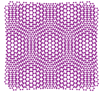
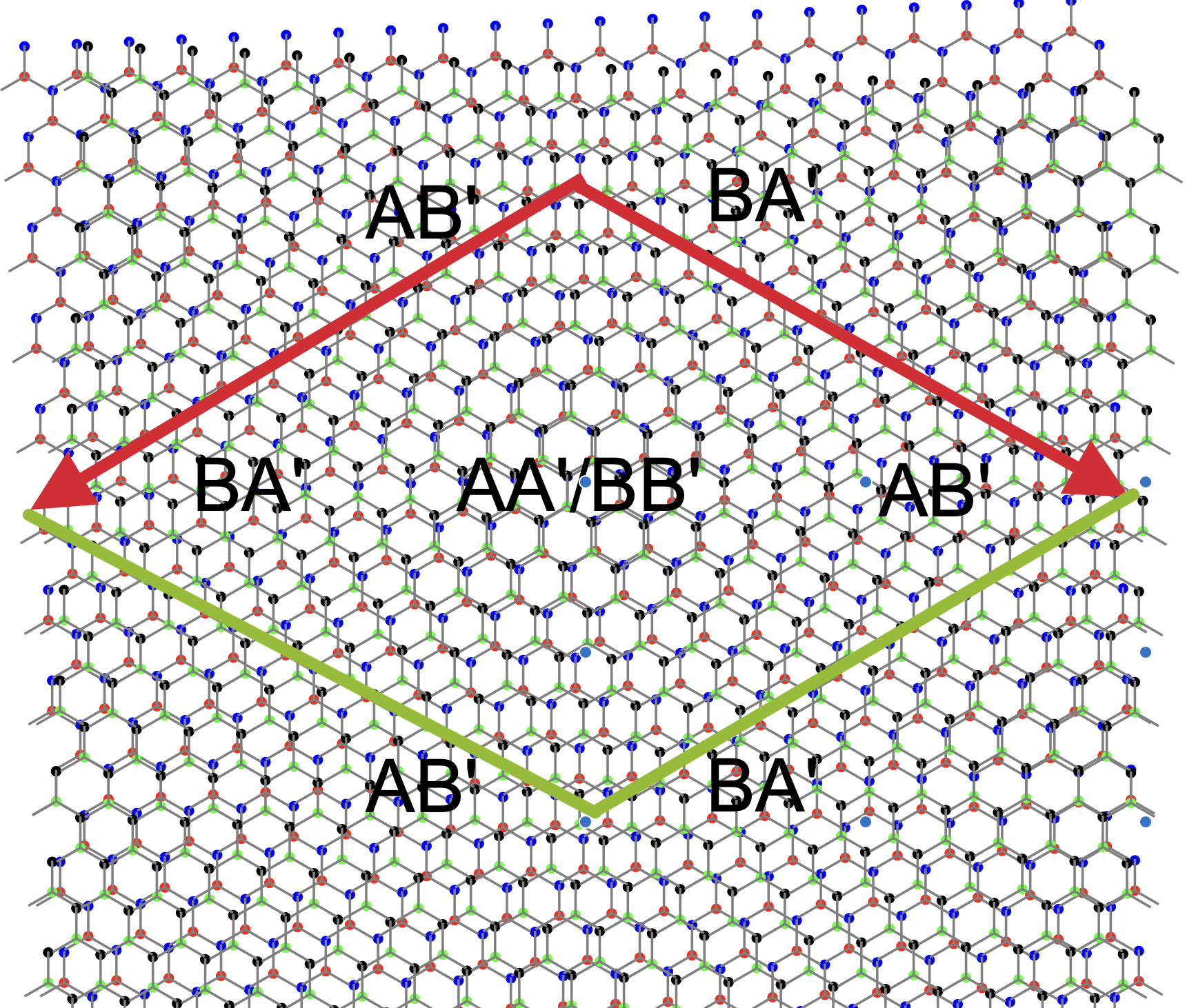
Figure 1. Left: Visible moiré pattern at $\theta=5^{\circ}$. Right: Single moiré hexagon, with (A=red, B=blue) and (A’=green, B’=black) denote vertices of two sheets of graphene respectively.

In the BM model, the bands near zero energy appear almost flat, while it has been discovered in [BEWZ20a, BEWZ20b, N21, NL22, TKV19] that the chiral limiting model exhibits perfectly flat bands at these so-called magic angles [BEWZ20a, TKV19] whereas the anti-chiral model does not exhibit flat bands [BEWZ20b]. In this article, we show that this dichotomy persists when a constant perpendicular magnetic field is applied §5.

In this paper, we first perform a spectral and symmetry analysis of our model for various magnetic perturbations. This includes the existence and absence of perfectly flat bands at magic angles for different interlayer potentials and magnetic fields, see also [BS99] for related results. This is shown in Section 5 in Theorem 6.

In this row of mathematically rigorous results, we also want to mention the computer-assisted proof of the existence of a real magic angle by Luskin and Watson [LW21] and other derivations of models for TBG [CGG22, Wa*22, CM23].

Our article is then structured as follows:

• In Section 2, we introduce the Bistritzer-MacDonald Hamiltonian for TBG with an additional external magnetic field.

• In Section 3, we introduce the magnetic Bloch-Floquet theory for the magnetic Bistritzer-MacDonald Hamiltonian.

• In Section 4, we specialize to the chiral limit and study the existence and Chern number of flat bands at zero energy in constant magnetic fields. In particular, Theorem 3 focuses on the non-magic-angle case; Theorem 4 and 5 focus on the simple and degenerate magic-angle case, respectively.

• In Section 5, we prove that for the magnetic BM model,

  • periodic magnetic fields do not affect the presence of flat bands in Theorem 6.

  • flat bands persist under rational (with respect to the lattice) magnetic flux in Theorem 7.

• In Section 6, we prove that a plethora of almost flat bands is located exponentially close to zero energy in Theorem 8. Finally, we conclude with some observations that show the presence of Landau-level type spectrum in the chiral model of twisted bilayer graphene in the absence of magnetic fields.

Acknowledgements. This research was partially supported by Simons 681675, NSF DMS-2052899 and DMS-2155211, DMS 2054589, and the Pacific Institute for the Mathematical Sciences. The contents of this work are solely the responsibility of the authors and do not necessarily represent the official views of PIMS.

2. Introduction of magnetic BM model

We start by introducing relevant notation.

Notation. We commonly identify ${\mathbb{R}}^{2}$ with ${\mathbb{C}}$ by writing $x=(x_{1},x_{2})$ also as $z=x_{1}+ix_{2}$. We write $f=\mathcal{O}_{\alpha}(g)_{H}$ if there is a constant $C_{\alpha}>0$ such that $\|f\|_{H}\leq C_{\alpha}g$. We add the subscript ${\mathbb{C}}_{z}$ or ${\mathbb{C}}_{\mathbf{k}}$ to refer to complex plane of variable $z$ or ${\mathbf{k}}$ when it is ambiguous in the context.

Given two vector space $A$ and $B$, we use $A\otimes B$ to denote the tensor product; $A\times B=\{(a,b):a\in A,b\in B\}$ to denote the direct product. Given a real (or complex) vector space $V$ and two subspaces $A,B\subset V$, we use $A\oplus B=\{c_{1}a+c_{2}b:c_{1},c_{2}\in{\mathbb{R}}\text{~{}(or~{}}{\mathbb{C}}),a\in A,b\in B\}$ to denote the inner direct sum. Denote $0_{{\mathbb{C}}^{2}}=(0,0)^{T}\in{\mathbb{C}}^{2}$.

2.1. Moiré lattices and TBG

When two honeycomb lattices are stacked on top of each other and twisted by an angle $\theta$, a moiré honeycomb pattern becomes visible, cf. Fig. 1. This new honeycomb structure has length scale $\lambda_{\theta}.$

To simplify the discussion, we start by introducing a unit-size honeycomb lattices, i.e. the one with side length $\frac{4\pi}{\sqrt{3}}$.

Let $\omega=\exp(\frac{2\pi i}{3})$, $\zeta_{1}=\frac{4\pi i\omega}{3}$ and $\zeta_{2}=\frac{4\pi i\omega^{2}}{3}$. A unit-size honeycomb lattice is then invariant under translations by the triangular lattice $\Gamma=\zeta_{1}{\mathbb{Z}}\oplus\zeta_{2}{\mathbb{Z}}$. The unit cell, its dual lattice, and the unit cell of the dual lattice (Brillouin zone) are denoted by $E={\mathbb{C}}/\Gamma$, $\Gamma^{*}=\eta_{1}{\mathbb{Z}}\oplus\eta_{2}{\mathbb{Z}}$, and $E^{*}={\mathbb{C}}/\Gamma^{*}$, respectively, where $\eta_{1}=\sqrt{3}\omega^{2}$ and $\eta_{2}=-\sqrt{3}\omega$. Since the moiré honeycomb lattice changes its length scale depending on the twisting angle, we also define a rescaled honeycomb lattice with scaling parameter $\lambda\in\mathbb{Z}^{2}$ by $\Gamma_{\lambda}=\lambda_{1}\zeta_{1}{\mathbb{Z}}\oplus\lambda_{2}\zeta_{2}{\mathbb{Z}}$, $E_{\lambda}={\mathbb{C}}/\Gamma_{\lambda}$, $\Gamma_{\lambda}^{*}=\lambda_{1}^{-1}\eta_{1}{\mathbb{Z}}\oplus\lambda_{2}^{-1}\eta_{2}{\mathbb{Z}}$ and $E_{\lambda}^{*}={\mathbb{C}}/\Gamma_{\lambda}^{*}$. Finally, we denote by $T_{1,\lambda},T_{2,\lambda}\in\mathcal{L}(L^{2}(\mathbb{C}))$ the standard translation operators $(T_{j,\lambda}u)(z):=u(z+\lambda_{j}\zeta_{j})$ associated with the lattice $\Gamma_{\lambda}$. In particular, when $\lambda_{j}=1$, we denote $(T_{j}u)(z):=u(z+\zeta_{j})$.

2.2. Chiral and anti-chiral limits

The two basic examples of tunneling potentials, $U$ and $V$, are defined as

$$U(z)=\sum_{\ell=0}^{2}\omega^{\ell}\exp\left(\frac{z\bar{\omega}^{\ell}-\bar{z}\omega^{\ell}}{2}\right),\quad V(z)=\sum_{\ell=0}^{2}\exp\left(\frac{z\bar{\omega}^{\ell}-\bar{z}\omega^{\ell}}{2}\right).$$

For ${\mathbf{a}}=n_{1}\zeta_{1}+n_{2}\zeta_{2}$, the potentials are defined to satisfy the following symmetries

$$\begin{split}&V(z+{\mathbf{a}})=\bar{\omega}^{n_{1}+n_{2}}V(z),\ \ V(\omega z)=V(z),\ \ V(\bar{z})=\overline{V(z)}=V(-z),\\ &U(z+\mathbf{a})=\bar{\omega}^{n_{1}+n_{2}}U(z),\ \ U(\omega z)=\omega U(z),\ \ U(\bar{z})=\overline{U(z)},\ \ U_{-}(z):=U(-z).\end{split}$$ (2.1)

(a) tunneling potential $|V|^{2}$ for $\mathrm{AA^{\prime}}/\mathrm{BB^{\prime}}$-coupling.

(b) tunneling potential $|U|^{2}$ for $\mathrm{AB^{\prime}}$-coupling.

(c) tunneling potential $|U_{-}|^{2}$ for $\mathrm{BA^{\prime}}$-coupling.

Figure 2. The tunneling potentials for different coupling types on unit-size honeycomb lattice.

2.3. Spectral properties of chiral and anti-chiral model

We start by introducing two different limiting cases of the BM Hamiltonian:

The chiral model is the Hamiltonian (1.1) when $\alpha_{0}=0$. When conjugated by the unitary $\mathscr{U}=\operatorname{diag}(1,\sigma_{1},1)$, $H_{\operatorname{c}}(\alpha_{1},B):=\mathscr{U}H\mathscr{U}$ has off-diagonal form

$$\begin{split}H_{\operatorname{c}}(\alpha_{1},B)&=\begin{pmatrix}0&(D_{c}(\alpha_{1},B))^{*}\\ D_{c}(\alpha_{1},B)&0\end{pmatrix}\text{ with }D_{c}(\alpha_{1},B)=\begin{pmatrix}a&\alpha_{1}U(z)\\ \alpha_{1}U_{-}(z)&a\end{pmatrix},\end{split}$$ (2.2)

where $a=2D_{\bar{z}}-A(z).$

The other limiting model is the anti-chiral model which is obtained by setting $\alpha_{1}=0$. It can also be transformed into an off-diagonal form when conjugated by a unitary $\mathcal{V}$, giving rise to a Hamiltonian

$$\begin{split}&H_{{\operatorname{ac}}}(\alpha_{0},B):=\mathcal{V}H\mathcal{V}=\begin{pmatrix}0&(D^{\theta}_{{\operatorname{ac}}}(\alpha_{0},B))^{*}\\ D^{\theta}_{{\operatorname{ac}}}(\alpha_{0},B)&0\end{pmatrix}\text{ with }\\ &D_{{\operatorname{ac}}}^{\theta}(\alpha_{0},B)=\begin{pmatrix}\alpha_{0}V(z)&e^{i\theta/2}a\\ e^{i\theta/2}a^{*}&\alpha_{0}\overline{V(z)}\end{pmatrix}\text{ where }\\ &\mathcal{V}=\begin{pmatrix}\mathcal{V}_{1}&\mathcal{V}_{2}\\ \mathcal{V}_{2}&\mathcal{V}_{1}\end{pmatrix}\text{ for }\mathcal{V}_{1}=\operatorname{diag}(i\lambda,0),\ \ \mathcal{V}_{2}=\operatorname{diag}(0,-\bar{\lambda}),\ \ \lambda=e^{i\frac{\pi}{4}}.\end{split}$$ (2.3)

Both the chiral and anti-chiral model can be cast in an off-diagonal matrix form. This implies that for both the chiral and anti-chiral model with magnetic field, the spectrum is symmetric with respect to zero. To see this directly, let $U:=(\sigma_{3}\otimes\operatorname{id}_{{\mathbb{C}}^{2}})$, then by directly conjugating the Hamiltonians, we find $UH_{c}U=-H_{c}$ and $UH_{{\operatorname{ac}}}^{\theta}U=-H_{{\operatorname{ac}}}^{\theta}.$

2.4. Characterization of magic angles

It has been shown [BEWZ20a] that in the absence of magnetic fields, i.e. $A=0$, there exists a discrete set $\mathcal{A}\subset\mathbb{C}$, the set of magic angles, such that for $\alpha_{1}\in\mathcal{A}$, the chiral model $H_{c}(\alpha_{1},B=0)$ (2.2) exhibits flat bands at energy zero.

More explicitly, this set $\mathcal{A}$ has been characterized by the eigenvalues of a compact operator

$$\begin{split}&\alpha_{1}\in\mathcal{A}\Leftrightarrow\alpha_{1}^{-1}\in\operatorname{Spec}(T_{\mathbf{k}})\text{ for some }\mathbf{k}\notin 3\Gamma^{*}\\ &T_{\mathbf{k}}=(2D_{\bar{z}}-\mathbf{k})^{-1}\begin{pmatrix}0&U(z)\\ U(-z)&0\end{pmatrix}:L^{2}_{0}({\mathbb{C}}/\Gamma)\to L^{2}_{0}({\mathbb{C}}/\Gamma).\end{split}$$

The space $L^{2}_{0}({\mathbb{C}}/\Gamma)$ is defined as

$$L^{2}_{0}({\mathbb{C}}/\Gamma):=\{u\in L^{2}({\mathbb{C}}/\Gamma);L_{a}u=u\text{ with }a\in\tfrac{\Gamma}{3}\}$$

where $L_{a}u(z)=\operatorname{diag}(\omega^{a_{1}+a_{2}},1)u(z+a)$ with $a=\frac{4}{3}\pi i(\omega a_{1}+\omega^{2}a_{2})$ for $a_{j}\in{\mathbb{Z}}.$

3. Magnetic Bloch-Floquet theory

In this section, we introduce the magnetic Bloch-Floquet theory following [Sj89] in preparation of studying the flat bands.

Bloch-Floquet theory yields a decomposition of an operator $S$ with translational symmetries with respect to a lattice, say $\Gamma$, into a family of simpler operators $\{S_{\mathbf{k}}\}_{{\mathbf{k}}\in{\mathbb{C}}/\Gamma^{*}}$. To obtain such a decomposition, we first need to find an Abelian group of translations $\{T_{{\mathbf{n}}}\}_{{\mathbf{n}}\in{\mathbb{Z}}^{2}}$ on $\Gamma$ that commute with $S$. Using these translations, one can construct a unitary operator, called the Gelfand transform $U$, such that $USU^{-1}=\int^{\oplus}_{{\mathbb{C}}/\Gamma^{*}}S_{\mathbf{k}}d{\mathbf{k}}$.

Assumption 1 (Magnetic potential).

We assume that the magnetic potential is of the form $A=A_{\operatorname{con}}+A_{\operatorname{per}}$, where

1. $A_{\operatorname{con}}(z)=\frac{Bi}{2}z$ generates a constant magnetic field $B$,

2. $A_{\operatorname{per}}$ is real-analytic and periodic w.r.t. $\Gamma_{\lambda}=\lambda_{1}\zeta_{1}{\mathbb{Z}}\oplus\lambda_{2}\zeta_{2}{\mathbb{Z}}$, for some $\lambda=(\lambda_{1},\lambda_{2})\in{\mathbb{Z}}^{2}$,

such that $\Phi_{\operatorname{mag}}:=B|{\mathbb{C}}/\Gamma_{\lambda}|\in 2\pi{\mathbb{Z}}$. In particular, we denote

$$v_{j}:=\lambda_{j}\zeta_{j},\ \Gamma_{\operatorname{mag}}:=\Gamma_{\lambda},\ p:=\frac{\Phi_{\operatorname{mag}}}{2\pi},\ q:=\lambda_{1}\lambda_{2},\text{~{}and~{}}\Phi:=B|{\mathbb{C}}/\Gamma|=2\pi\tfrac{p}{q}\in 2\pi\mathbb{Q},$$ (3.1)

for some $p,q\in{\mathbb{Z}}$. The integer $p$ is called the number of Dirac flux quanta.

We start by defining magnetic translations on $\Gamma_{\operatorname{mag}}=v_{1}{\mathbb{Z}}\oplus v_{2}{\mathbb{Z}}$. To this end, recall that the standard translation by $v_{j}$ have been denoted by $T_{j,\lambda}$ in Sec 2.1. Then the basic magnetic translation by $v_{j}$ can be defined as

$$T_{j,\text{mag}}:=e^{i\varphi_{j}}T_{j,\lambda}\text{~{}with~{}}\varphi_{j}(z)=-\operatorname{Re}(\overline{A_{\operatorname{con}}(v_{j})}z),\quad j=1,2,$$ (3.2)

which satisfy $2D_{z}(i\varphi_{j})=-\overline{A_{\operatorname{con}}(v_{j})}$ and $2D_{\bar{z}}(i\varphi_{j})=-A_{\operatorname{con}}(v_{j})$ such that

$$[a^{*},T_{j,\text{mag}}]=[a,T_{j,\text{mag}}]=0,\quad\text{where~{}}a=2D_{\bar{z}}-A(z).$$ (3.3)

Furthermore, for our model, $A_{\operatorname{con}}(z)=\frac{Biz}{2}$ implies $\varphi_{j}(z)=\frac{Bi}{4}(\overline{v_{j}}z-v_{j}\bar{z})$ is linear in $z$ and $\bar{z}$. Thus we can see

$$\begin{split}T_{1,{\operatorname{mag}}}T_{2,{\operatorname{mag}}}&=e^{i\varphi_{1}+i\varphi_{2}(\bullet+v_{1})}T_{1,\lambda}T_{2,\lambda}=e^{i(\varphi_{2}(v_{1})-\varphi_{1}(v_{2}))}e^{i\varphi_{2}+i\varphi_{1}(\bullet+v_{2})}T_{2,\lambda}T_{1,\lambda}\\ &=e^{i(\varphi_{2}(v_{1})-\varphi_{1}(v_{2}))}T_{2,{\operatorname{mag}}}T_{1,{\operatorname{mag}}}\\ &=e^{-\frac{B}{2}(\overline{v_{1}}v_{2}-\overline{v_{2}}v_{1})}T_{2,\text{mag}}T_{1,\text{mag}}\\ &=e^{-iB|{\mathbb{C}}/\Gamma_{\operatorname{mag}}|}T_{2,{\operatorname{mag}}}T_{1,{\operatorname{mag}}}=e^{-2\pi pi}T_{2,{\operatorname{mag}}}T_{1,{\operatorname{mag}}}=T_{2,{\operatorname{mag}}}T_{1,{\operatorname{mag}}}.\end{split}$$ (3.4)

where we used $\overline{v_{1}}v_{2}-\overline{v_{2}}v_{1}=2i|{\mathbb{C}}/\Gamma_{\operatorname{mag}}|$.

The commutativity of translations above allows us then to define general magnetic translation on $\Gamma_{\operatorname{mag}}$:

$$T_{\textbf{n},\text{mag}}:=T_{1,\text{mag}}^{n_{1}}T_{2,\text{mag}}^{n_{2}}\text{~{}for~{}}\textbf{n}=(n_{1},n_{2})\in{\mathbb{Z}}^{2}.$$ (3.5)

By (3.3) and (3.4), we have for $\textbf{n},\textbf{n}^{\prime}\in{\mathbb{Z}}^{2}$,

$$\begin{split}&T_{\textbf{n},\text{mag}}T_{\textbf{n}^{\prime},\text{mag}}=T_{\textbf{n}+\textbf{n}^{\prime},\text{mag}}=T_{\textbf{n}^{\prime},\text{mag}}T_{\textbf{n},\text{mag}},\text{~{}and~{}}\\ &[T_{{\mathbf{n}},\text{mag}},a]=[T_{{\mathbf{n}},\text{mag}},a^{*}]=0.\end{split}$$ (3.6)

Thus, $\{T_{\textbf{n},\text{mag}}\}_{\textbf{n}\in{\mathbb{Z}}^{2}}$ forms an abelian group of translations on $\Gamma_{\operatorname{mag}}$ that commutes with $a$ and $a^{*}$.

Furthermore, $T_{{\mathbf{n}},\text{mag}}$ gives rises to Abelian groups that commute with many more complicated operators. We summarize them all below:

Lemma 3.1.

Let $A$ satisfy Assumption 1. Let $T_{{\mathbf{n}},\operatorname{mag}}$ be defined as in (3.5). Then the following families of translations form Abelian groups and

1. $\{T_{{\mathbf{n}},\operatorname{mag}}:{\mathbf{n}}\in{\mathbb{Z}}^{2}\}$ commutes with $a,a^{*}$ in (1.1),

2. $\{\operatorname{diag}(1,1)\otimes T_{{\mathbf{n}},\operatorname{mag}}:{\mathbf{n}}\in{\mathbb{Z}}^{2}\}$ commutes with $H_{D}^{B}$ in (1.1),

3. $\{\operatorname{diag}(\omega^{{\mathbf{n}}\cdot\lambda},\omega^{{\mathbf{n}}\cdot\lambda},1,1)\otimes T_{{\mathbf{n}},\operatorname{mag}}:{\mathbf{n}}\in{\mathbb{Z}}^{2}\}$ commutes with $H$ in (1.1),

4. $\{\operatorname{diag}(\omega^{{\mathbf{n}}\cdot\lambda},1)\otimes T_{{\mathbf{n}},\operatorname{mag}}:{\mathbf{n}}\in{\mathbb{Z}}^{2}\}$ commutes with $D_{\text{c}}(\alpha_{1},B)$ in (2.2),

5. $\{\operatorname{diag}(\omega^{{\mathbf{n}}\cdot\lambda},1,\omega^{{\mathbf{n}}\cdot\lambda},1)\otimes T_{{\mathbf{n}},\operatorname{mag}}:{\mathbf{n}}\in{\mathbb{Z}}^{2}\}$ commutes with $H_{\text{c}}(\alpha_{1},B)$ in (2.2),

6. $\{\operatorname{diag}(-\omega^{{\mathbf{n}}\cdot\lambda},-1,1,-\omega^{{\mathbf{n}}\cdot\lambda})\otimes T_{{\mathbf{n}},\operatorname{mag}}:{\mathbf{n}}\in{\mathbb{Z}}^{2}\}$ commutes with $H_{\text{ac}}(\alpha_{0},B)$ in (2.2),

where ${\mathbf{n}}\cdot\lambda:=n_{1}\lambda_{1}+n_{2}\lambda_{2}$, $\omega=\exp(\tfrac{2\pi i}{3})$.

Proof.

$(1)$ has already been established in (3.3). For the remaining parts, by (2.1) and (3.2), we have

$$\begin{cases}XT_{{\mathbf{n}},\text{mag}}=\omega^{{\mathbf{n}}\cdot\lambda}T_{{\mathbf{n}},\text{mag}}X,&\text{~{}for~{}}X\in\{U(z),V(z),\overline{U_{-}}(z)\},\\ YT_{{\mathbf{n}},\text{mag}}=\omega^{{\mathbf{n}}\cdot\lambda}T_{{\mathbf{n}},\text{mag}}Y,&\text{~{}for~{}}Y\in\{\overline{U}(z),\overline{V}(z),U_{-}(z)\}.\end{cases}$$ (3.7)

Then the claims follow by definition and direct computation. ∎

In particular, throughout the article, we will abuse the notation in the following way: When the operator is clearly specified, we will use the same notation $\mathscr{L}_{\mathbf{n}}$ to denote the translations above for the corresponding operators. For example, the $\mathscr{L}_{\mathbf{n}}$ for $H_{c}(\alpha_{1},B)$ will be $\mathscr{L}_{\mathbf{n}}=\operatorname{diag}(\omega^{{\mathbf{n}}\cdot\lambda},1,\omega^{{\mathbf{n}}\cdot\lambda},1)\otimes T_{{\mathbf{n}},\operatorname{mag}}$.

Furthermore, we will build up the general Bloch-Floquet theory using this kind of (abused) general notation. The $\mathcal{H}_{f}$, $\mathcal{H}_{\tau}$, $\mathcal{U}_{B}$ below all depends on the operator but will be abused throughout the paper when the corresponding operator is clear.

Theorem 1 (Magnetic Bloch-Floquet theory).

Assume $\{\mathscr{L}_{\mathbf{n}}\}_{{\mathbf{n}}\in{\mathbb{Z}}^{2}}$ form a family of translations, as specified in Lemma 3.1, commuting with some operator $S=S(z,\bar{z},D_{z},D_{\bar{z}})$ on $L^{2}({\mathbb{C}};{\mathbb{C}}^{d})$. Then, we define the Hilbert space

$$\mathcal{H}_{f}:=\{f\in L^{2}_{\operatorname{loc}}({\mathbb{C}};{\mathbb{C}}^{d});\mathscr{L}_{\mathbf{n}}f(z)=f(z)\text{ for all }\textbf{n}\in\mathbb{Z}^{2}\}$$ (3.8)

which naturally defines a Hilbert space with inner product $\langle f,g\rangle_{\mathcal{H}_{f}}:=\int_{{\mathbb{C}}/\Gamma_{\operatorname{mag}}}\langle f(y),g(y)\rangle_{{\mathbb{C}}^{d}}\ dy$. We then define the Hilbert space

$$\mathcal{H}_{\tau}:=\{f\in L^{2}_{\operatorname{loc}}({\mathbb{C}};\mathcal{H}_{f});f(\mathbf{k}-\gamma^{*},z)=e^{-i\operatorname{Re}(z\bar{\gamma}^{*})}f(\mathbf{k},z)\text{ for all }\gamma^{*}\in\Gamma^{*}_{\operatorname{mag}}\}.$$

The Gelfand transform $\mathcal{U}_{B}:L^{2}({\mathbb{C}})\to\mathcal{H}_{\tau}$ is defined for $u\in C_{c}({\mathbb{C}})$ by

$$\mathcal{U}_{B}u(\mathbf{k},z):=\sum_{\mathbf{n}\in{\mathbb{Z}}^{2}}e^{-i\operatorname{Re}((n_{1}v_{1}+n_{2}v_{2}-z)\overline{\mathbf{k}})}(\mathscr{L}_{\mathbf{n}}u)(z)$$

and extends to a unitary operator with inverse

$$\mathcal{U}_{B}^{-1}\phi(z)=\int_{{\mathbb{C}}/\Gamma^{*}_{\operatorname{mag}}}e^{-i\operatorname{Re}(z\overline{\mathbf{k}})}\phi(\mathbf{k},z)\frac{d\mathbf{k}}{|{\mathbb{C}}/\Gamma^{*}_{\operatorname{mag}}|},$$

such that for fiber operators $S_{\mathbf{k}}(z,\bar{z},D_{z},D_{\bar{z}}):=S(z,\bar{z},D_{z}+\tfrac{\overline{\mathbf{k}}}{2},D_{\bar{z}}+\tfrac{\mathbf{k}}{2})$ on $\mathcal{H}_{f}$

$$\mathcal{U}_{B}S\ \mathcal{U}_{B}^{*}=\int^{\oplus}_{{\mathbb{C}}/\Gamma_{\operatorname{mag}}^{*}}S_{\mathbf{k}}(z,\bar{z},D_{z},D_{\bar{z}})\ d\mathbf{k}.$$

Remark 1.

The magnetic Sobolev spaces associated with (3.8), when working with operators mentioned in Lemma 3.1, are defined for $m\in\mathbb{N}$ as

$$H^{m}_{\mathcal{H}_{f}}:=\{f\in\mathcal{H}_{f};(a^{*})^{\alpha_{1}}a^{\alpha_{2}}f\in\mathcal{H}_{f},|\alpha|\leq m\},$$

with inner product

$$\langle f,g\rangle_{H^{m}_{\mathcal{H}_{f}}}:=\sum_{|\alpha|\leq m}\langle(a^{*})^{\alpha_{1}}a^{\alpha_{2}}f,(a^{*})^{\alpha_{1}}a^{\alpha_{2}}g\rangle_{\mathcal{H}_{f}}.$$

We first consider the case when $A_{\operatorname{per}}=0$. Notice that the fiber operators of $a=2D_{\bar{z}}-A(z)$ are $a_{\mathbf{k}}=a+{\mathbf{k}}$. Furthermore, for $A(z)=\frac{Bi}{2}z$, we have $[a_{\mathbf{k}},a_{\mathbf{k}}^{*}]=2B.$ This implies that $\ker_{\mathcal{H}_{f}}(a_{\mathbf{k}})=\{0\}$ for $B<0$ and $\ker_{\mathcal{H}_{f}}(a_{\mathbf{k}}^{*})=\{0\}$ for $B>0.$ We shall next construct $\operatorname{ker}_{\mathcal{H}_{f}}(a_{\mathbf{k}})$ for $B>0.$

Before we start, let us recall the nullspace of $a_{\mathbf{k}}$ on $L^{2}({\mathbb{C}})$. Due to the conjugacy relation $a_{\mathbf{k}}=e^{-\frac{i{\mathbf{k}}\bar{z}}{2}}e^{-B|z|^{2}/4}(2D_{\bar{z}})e^{B|z|^{2}/4}e^{\frac{ik\bar{z}}{2}}$, this is precisely the (transformed) Bargmann space

$$\text{ker}_{L^{2}({\mathbb{C}})}(a_{\mathbf{k}})=\left\{e^{-\frac{i{\mathbf{k}}\bar{z}}{2}}e^{-B|z|^{2}/4}f(z);f\in\mathscr{O}({\mathbb{C}}),\int_{{\mathbb{C}}}|f(z)|^{2}e^{-B|z|^{2}/2}\ dz<\infty\right\},$$ (3.9)

where $\mathscr{O}({\mathbb{C}})$ is the set of entire functions.

While the characterization of the nullspace of $a_{\mathbf{k}}$ , and thus of $H_{D}^{B}$, on $L^{2}({\mathbb{C}})$ is straightforward and perhaps well-known as above, we will need the nullspace of $a_{\mathbf{k}}$ and $H_{D,\mathbf{k}}^{B}$ on the magnetic torus ${\mathbb{C}}/\Gamma_{\operatorname{mag}}$ associated with the honeycomb lattice, instead. In another words, we need $\ker_{\mathcal{H}_{f}}(a_{\mathbf{k}})$ rather than $\ker_{L^{2}({\mathbb{C}})}(a_{\mathbf{k}})$. As we will see, the ansatz of finding $\ker_{\mathcal{H}_{f}}(a_{\mathbf{k}})$ is inspired by the structure of $\ker_{L^{2}({\mathbb{C}})}(a_{\mathbf{k}})$.

Theorem 2.

Assume $A(z)$ satisfy Assumption 1 with $A_{\operatorname{per}}=0$ and $B>0$, we have $\ker(a_{\mathbf{k}}^{*})=\{0\}$ while $\ker_{\mathcal{H}_{f}}(a_{\mathbf{k}})$ is composed of functions

$$u_{\mathbf{k}}(z)=e^{-\frac{i\mathbf{k}\bar{z}}{2}}e^{B\frac{(z^{2}-|z|^{2})}{4}}g(z)$$ (3.10)

with $g(z)=e^{\gamma z}\prod\limits_{i=1}^{p}\tilde{\sigma}(z-z_{i})$ for arbitrary $\gamma\in{\mathbb{C}}$ and $z_{i}\in{\mathbb{C}}$ satisfying the following two constraint equations

$$\gamma v_{j}-i\frac{\mathbf{k}\overline{v_{j}}}{2}+ip\pi=\xi_{j}\sum_{j=1}^{p}z_{j},\qquad j\in\{1,2\}.$$ (3.11)

Here $v_{j}:=\lambda_{j}\zeta_{j}$, $\xi_{j}:=\frac{2\pi i\lambda_{j}B}{3}$ and $\tilde{\sigma}$ is the modular-invariant Weierstraß function, as defined in [H18]. In particular, $\dim\ker_{\mathcal{H}_{f}}(a_{\mathbf{k}})=p$.

Finally, $a_{\mathbf{k}}$ is a Fredholm operator of index

$$\operatorname{ind}(a_{\mathbf{k}})=\operatorname{dim}\ker_{\mathcal{H}_{f}}(a_{\mathbf{k}})-\operatorname{dim}\ker_{\mathcal{H}_{f}}(a^{*}_{{\mathbf{k}}})=p$$

and $\ker_{\mathcal{H}_{f}\times\mathcal{H}_{f}}(H_{D,\mathbf{k}}^{B})=\ker_{\mathcal{H}_{f}}(a_{\mathbf{k}})\times\{0\}.$

Proof.

We start with the ansatz $u_{\mathbf{k}}(z)=e^{-\frac{i\mathbf{k}\bar{z}}{2}}e^{B\frac{(z^{2}-|z|^{2})}{4}}g(z)$, inspired by the nullspace of $a$ on $L^{2}({\mathbb{C}})$ in (3.9), where $g$ is an entire function that we will determine soon.

Recall that $v_{j}=\lambda_{j}\zeta_{j}$, and our ansatz $u_{\mathbf{k}}$ satisfies $T_{j,\text{mag}}u_{\mathbf{k}}(z)=u_{\mathbf{k}}(z)$, i.e.

$$\begin{split}1&=\frac{T_{j,\text{mag}}u_{k}}{u_{k}}=\frac{e^{i\varphi_{j}(z)}u_{\mathbf{k}}(z+v_{j})}{u_{\mathbf{k}}(z)}\\ &=\frac{g(z+v_{j})}{g(z)}\exp\left(\tfrac{B}{4}(v_{j}\bar{z}-\overline{v_{j}}z)-\tfrac{i{\mathbf{k}}\overline{v_{j}}}{2}+\tfrac{B}{4}(v_{j}^{2}+2v_{j}z-|v_{j}|^{2}-z\overline{v_{j}}-\overline{z}v_{j})\right)\\ &=\frac{g(z+v_{j})}{g(z)}\exp\left(-\tfrac{i{\mathbf{k}}\overline{v_{j}}}{2}+\tfrac{Bz}{2}(\overline{v_{j}}-v_{j})+\tfrac{Bv_{j}}{4}(\overline{v_{j}}-v_{j})\right).\end{split}$$

Thus we get the boundary constraints of $g(z)$ on the unit cell ${\mathbb{C}}/\Gamma_{\text{mag}}$:

$$g(z+v_{j})=g(z)\exp\left(\tfrac{i{\mathbf{k}}\overline{v_{j}}}{2}+\xi_{j}z+S_{j}\right),$$ (3.12)

where $\xi_{j}=\tfrac{B}{2}(\overline{v_{j}}-v_{j})=\tfrac{2\pi iB\lambda_{j}}{3}$ and $S_{j}=\tfrac{\xi_{j}v_{j}}{2}$.

To find entire functions $g(z)$ satisfying (3.12), we first count the number of zeros of $g$ by the argument principle. By $\overline{v_{1}}v_{2}-\overline{v_{2}}v_{1}=2i|{\mathbb{C}}/\Gamma_{\text{mag}}|$ and (3.1), we have

$$\begin{split}\frac{1}{2\pi i}\int_{\partial({\mathbb{C}}/\Gamma_{\operatorname{mag}})}\frac{g^{\prime}(z)}{g(z)}\ dz&=\frac{1}{2\pi i}\left(\int_{\frac{-v_{1}+v_{2}}{2}}^{-\frac{v_{1}+v_{2}}{2}}d\left(\log\tfrac{g(z)}{g(z+v_{1})}\right)+\int_{-\frac{v_{1}+v_{2}}{2}}^{\frac{v_{1}-v_{2}}{2}}d\left(\log\tfrac{g(z)}{g(z+v_{2})}\right)\right)\\ &=\frac{v_{2}\xi_{1}-v_{1}\xi_{2}}{2\pi i}=\frac{B(\overline{v_{1}}v_{2}-\overline{v_{2}}v_{1})}{4\pi i}=\frac{2Bi|{\mathbb{C}}/\Gamma_{\text{mag}}|}{4\pi i}=p.\end{split}$$ (3.13)

Hence $g$ has $p$ zeros (counting multiplicity) in a unit cell ${\mathbb{C}}/\Gamma_{\operatorname{mag}}$. We denote them by $z_{1},\dots,z_{p}$. We also denote the non-repeated zeros of $g$ by $w_{1},\dots,w_{p_{0}}$ with multiplicity $n_{1},\dots,n_{p_{0}}$, where $n_{1}+\dots+n_{p_{0}}=p$.

To determine $g$, we further notice that, by the boundary constraints (3.12),

$$\frac{g^{\prime}(z+v_{j})}{g(z+v_{j})}=\frac{g^{\prime}(z)}{g(z)}+\xi_{j},\qquad j=1,2.$$

As a result, $f:=(g^{\prime}/g)^{\prime}$ is a meromorphic, double periodic function; thus, an elliptic function. Furthermore, $f$ has (and only has) a pole of order $2$ at each (non-repeated) zero of $g$, i.e. $w_{i}$, $i=1,\dots,p_{0}$. Such kind of elliptic function with poles of order $2$ can be constructed using the so-called Weierstraß $\wp$-function

$$\wp(z)=\frac{1}{z^{2}}+\sum\limits_{\gamma\in\Gamma_{\text{mag}}^{\times}}\left(\frac{1}{(z-\gamma)^{2}}-\frac{1}{\gamma^{2}}\right),\quad\text{~{}where~{}}\Gamma_{\text{mag}}^{\times}=\Gamma_{\text{mag}}\setminus\{0\}.$$

The Weierstraß $\wp$-function is double periodic w.r.t. $\Gamma_{\text{mag}}$, holomorphic on ${\mathbb{C}}\setminus\Gamma_{\text{mag}}$, and has poles of order $2$ at lattice points $\Gamma_{\text{mag}}$. From $\wp$, we can construct $f$ in the following way:

Denote the Laurent expansion of $f$ near each $w_{i}$ as $f(z)=\sum\limits_{k=-2}^{+\infty}c_{k}^{(i)}(z-w_{i})^{k}$. Since $w_{i}$ is a zero of order $n_{i}$ for $g$, we see that

$$c_{-2}^{(i)}=\lim\limits_{z\to w_{i}}f(z)(z-w_{i})^{2}=\lim\limits_{z\to w_{i}}\left(\frac{g^{\prime}(z)}{g(z)}\right)^{\prime}(z-w_{i})^{2}=-n_{i}.$$

Then $F(z):=f(z)+\sum\limits_{i=1}^{p_{0}}n_{i}\wp(z-w_{i})$ has no poles anymore because $f$ and $\wp$ only have poles of order $2$ but they are all eliminated by the summation. As a result, $F(z)$ is entire, double periodic; thus, by Liouville’s theorem, a constant. We denote it by $c_{0}$. Hence we have

$$\left(\frac{d}{dz}\log(g(z))\right)^{\prime}=\left(\frac{g^{\prime}(z)}{g(z)}\right)^{\prime}=f(z)=-\sum_{i=1}^{p}n_{i}\wp(z-w_{i})+c_{0}.$$ (3.14)

To solve for $g$, recall that the Weierstraß sigma function (See Appendix A for more details)

$$\sigma(z)=z\prod_{\nu\in\Gamma_{\operatorname{mag}}^{\times}}\Big{(}1-\frac{z}{\nu}\Big{)}e^{\frac{z}{\nu}+\frac{z^{2}}{2\nu^{2}}}\quad\text{~{}satisfies~{}}\quad\left(\frac{d}{dz}\log(\sigma(z))\right)^{\prime}=\left(\frac{\sigma^{\prime}(z)}{\sigma(z)}\right)^{\prime}=-\wp(z).$$

Plug into (3.14) and integrate (3.14) twice, we get

$$\begin{split}&\log(g(z))=\sum\limits_{i=1}^{p_{0}}n_{i}\log(\sigma(z-w_{i}))+c_{0}z^{2}+c_{1}z+c_{2},\\ \Rightarrow\quad&g(z)=e^{c_{0}z^{2}+c_{1}z+c_{2}}\prod_{i=1}^{p_{0}}\left(\sigma(z-w_{i})\right)^{n_{i}}=:ce^{p(z)}\prod_{i=1}^{p_{0}}\left(\sigma(z-w_{i})\right)^{n_{i}}.\end{split}$$

To solve for $p$, we first recall the “modified” Weierstraß sigma function $\tilde{\sigma}(z)$, introduced by Haldane in [H18, eq. (11)], which has the following properties:

$$\tilde{\sigma}(z)=e^{-\frac{1}{2}\gamma_{2}(\Gamma_{\text{mag}})z^{2}}\sigma(z),\quad\text{~{}with~{}}\quad\tilde{\sigma}(z+v_{j})=-e^{\frac{\xi_{j}z+S_{j}}{p}}\tilde{\sigma}(z),\quad j=1,2.$$ (3.15)

where $\gamma_{2}(\Lambda)$ is a constant depending on the lattice $\Lambda$, see [H18, eq. (8)]. Then we also notice that $n_{i}$ is the multiplicity of the non-repeated zeros $w_{i}$. As a result, we can rewrite $g(z)$ as

$$g(z)=ce^{p(z)}\prod_{i=1}^{p_{0}}\left(\sigma(z-w_{i})\right)^{n_{i}}=\tilde{c}e^{\tilde{p}(z)}\prod_{i=1}^{p_{0}}\left(\tilde{\sigma}(z-w_{i})\right)^{n_{i}}=\tilde{c}e^{\tilde{p}(z)}\prod_{i=1}^{p}\tilde{\sigma}(z-z_{i})$$

for some other second degree polynomial $\tilde{p}(z)$. Denote $\tilde{p}(z)=\gamma_{2}z^{2}+\gamma_{1}z$ where the constant term is absorbed by $\tilde{c}$. Using the boundary constraints of $g$ in (3.12) and of $\tilde{\sigma}$ in (3.15), we find for $j=1,2$,

$$2\gamma_{2}v_{j}+\xi_{j}=\xi_{j},\qquad\Rightarrow\qquad\gamma_{2}=0,$$ (3.16)

$$\gamma_{1}v_{j}+i\pi p-\frac{\xi_{j}}{p}\sum\limits_{i=1}^{p}z_{i}=\frac{i{\mathbf{k}}\overline{v_{j}}}{2}.$$ (3.17)

Denote $Z_{p}:=\sum\limits_{i=1}^{p}z_{i}\in{\mathbb{C}}$. From (3.17) with $j=1,2$, we can solve for

$$\begin{split}\gamma_{1}&=\frac{ip\pi(\xi_{2}-\xi_{1})-\frac{{\mathbf{k}}i}{2}(\xi_{2}\overline{v_{1}}-\xi_{1}\overline{v_{2}})}{\xi_{1}v_{2}-\xi_{2}v_{1}}=i\frac{{\mathbf{k}}}{2}+i\frac{\pi B}{3}(\lambda_{2}-\lambda_{1}),\\ Z_{p}&=\frac{ip\pi(v_{1}-v_{2})-\frac{{\mathbf{k}}i}{2}(\overline{v_{2}}v_{1}-\overline{v_{1}}v_{2})}{\frac{1}{p}(\xi_{2}v_{1}-\xi_{1}v_{2})}=\frac{2\pi ip}{3}(\lambda_{2}\omega^{2}-\lambda_{1}\omega)-i\frac{{\mathbf{k}}p}{B}.\end{split}$$ (3.18)

In summary, $u_{\mathbf{k}}(z)=e^{-\frac{i{\mathbf{k}}\bar{z}}{2}}e^{B\frac{(z^{2}-|z|^{2})}{4}}g(z)\in\ker_{\mathcal{H}_{f}}(a_{\mathbf{k}})$ as long as $g(z)=\tilde{c}e^{\gamma_{1}z}\prod\limits_{i=1}^{p}\tilde{\sigma}(z-z_{i})$ with $\gamma_{1}$, $Z_{p}=\sum\limits_{i=1}^{p}z_{i}$ satisfy (3.18).

Now we determine the dimension of this space. Since the function exhibits precisely $p$ zeros, we can construct also $p$ linearly independent solutions, see e.g. [BHZ22b, Lemma $4.1$] for an analogous construction. There cannot be more solutions by the Riemann-Roch theorem:

Indeed, consider one possible solution $u_{{\mathbf{k}}}$ with fixed zeros at $z_{1},...,z_{p}$ and any other solution $v_{{\mathbf{k}}},$ then $\frac{v_{{\mathbf{k}}}}{u_{{\mathbf{k}}}}$ is a meromorphic function with (possible) poles at $z_{1},...,z_{p}.$ The Riemann-Roch theorem states that for the special case of the two-dimensional torus the dimension of the space of meromorphic functions with this fixed set of possible poles is equal to the number of poles, which is $p$.

For completeness, we recall that the non-zero energy bands of the magnetic Dirac operator are then derived by defining first

$$u_{\mathbf{k},n}:=\frac{(a^{*}_{\mathbf{k}})^{n}}{(2B)^{n/2}\sqrt{n!}}u_{\mathbf{k}},\quad n\in\mathbb{N}_{0},$$

with $u_{\mathbf{k}}\in\ker(a_{\mathbf{k}}).$ We then find

$$\begin{split}a_{\mathbf{k}}^{*}u_{\mathbf{k},n}&=\sqrt{2B(n+1)}\ u_{\mathbf{k},n+1}\text{ and }a_{\mathbf{k}}u_{\mathbf{k},n}=\sqrt{2Bn}\ u_{\mathbf{k},n-1}\end{split}.$$

This way, for $n\neq 0,$

$$\begin{split}H^{B}_{D,\mathbf{k}}\begin{pmatrix}\pm u_{\mathbf{k},n-1}\\ u_{\mathbf{k},n}\end{pmatrix}&=\pm\sqrt{2Bn}\begin{pmatrix}\pm u_{\mathbf{k},n-1}\\ u_{\mathbf{k},n}\end{pmatrix}.\end{split}$$ (3.19)

We can then use this to see that $a_{\mathbf{k}}$ is Fredholm on $\mathcal{H}_{f}$, i.e. possesses a finite-dimensional kernel and has closed range. This follows for example from the criterion stated in [T92, p.158 (footnote)]: The Hamiltonian $H_{D,\mathbf{k}}^{B}$ is Fredholm if and only if both $a_{\mathbf{k}}$ and $a_{\mathbf{k}}^{*}$ are. Meanwhile, by [T92, Theo $5.19$], $H_{D,\mathbf{k}}^{B}$ is Fredholm if and only if $e^{-(H_{D,\mathbf{k}}^{B})^{2}t}$ is trace-class for some $t>0$. The latter can be easily verified using (3.19). The Fredholm index

$$\operatorname{ind}_{\mathcal{H}_{f}}(a_{\mathbf{k}})=\operatorname{dim}\ker_{\mathcal{H}_{f}}(a_{\mathbf{k}})-\operatorname{dim}\ker_{\mathcal{H}_{f}}(a_{\mathbf{k}}^{*})$$

is readily computed from the dimension of the nullspaces of $a_{\mathbf{k}}$, which is $p$ and of $a_{\mathbf{k}}^{*}$, which is $0.$ ∎

Remark 2.

Let $(Qu)(z):=\overline{u(-z)}$. Recall that $A(z)=\frac{Bi}{2}z$. Then by direct computation,

$$Q(a_{\mathbf{k}})Q^{*}=Q(2D_{\overline{z}}-A(z)+{\mathbf{k}})Q=2D_{z}+\overline{A(z)}+\overline{{\mathbf{k}}}.$$

Thus $Qu_{\mathbf{k}}\in\ker_{\mathcal{H}_{f}}(2D_{z}+\overline{A(z)}+\overline{{\mathbf{k}}})$ for any $u_{\mathbf{k}}\in\ker_{\mathcal{H}_{f}}(a_{\mathbf{k}})$. Notice that $2D_{z}+\overline{A(z)}+\overline{{\mathbf{k}}}\neq a_{\mathbf{k}}^{*}=2D_{z}-\overline{A(z)}+\overline{{\mathbf{k}}}$. In fact, $2D_{z}+\overline{A(z)}+\overline{{\mathbf{k}}}=(a_{\mathbf{k}}(-B))^{*}$ where $a_{\mathbf{k}}(-B)=2D_{\bar{z}}+\frac{Bi}{2}z$ represents the negative constant magnetic field $-B$.

Remark 3.

If $\lambda_{1}=\lambda_{2}=1$ the last two equations (3.18) reduce to

$$\gamma_{1}=\frac{i\mathbf{k}}{2}\text{ and }Z_{p}=\frac{2\pi p}{\sqrt{3}}-\frac{4\pi i}{3\sqrt{3}}\mathbf{k}.$$ (3.20)

A direct consequence of Theorem 2 is, we can compute the Fredholm index for the chiral model.

Corollary 3.2.

Under the same assumptions as in Theorem 2, the operator $D_{c}(\alpha_{1},B)+\mathbf{k}$ on $\mathcal{H}_{f}$ is a Fredholm operator of index $2p.$

Proof.

We recall that the direct sum of Fredholm operators $\operatorname{diag}(a_{\mathbf{k}},a_{\mathbf{k}})$ is a Fredholm operator with twice the index of $a_{\mathbf{k}}$. Since $U,U_{-}$ are smooth functions, $\begin{pmatrix}0&\alpha_{1}U(z)\\ \alpha_{1}U_{-}(z)&0\end{pmatrix}$ is a relatively compact perturbation [T92, Prop.$5.27$] of $\operatorname{diag}(a_{\mathbf{k}},a_{\mathbf{k}})$ which does not affect the index. To summarize, we have argued that

$$\operatorname{ind}_{\mathcal{H}_{f}}(D_{c}(\alpha_{1},B)+\mathbf{k})=2\operatorname{ind}_{\mathcal{H}_{f}}(a_{{\mathbf{k}}})=2p.$$ (3.21)

∎

We also observe that every zero of elements in the nullspace of $D_{c}(\alpha_{1},B)+k$ are of $z$-type (and analogously for elements in the nullspace of $D_{c}(\alpha_{1},B)^{*}+\bar{k}$ are of $\bar{z}$-type).

Lemma 3.3.

Let $w\in C^{\infty}({\mathbb{C}};{\mathbb{C}}^{2})$ and that $(D_{c}(\alpha_{1},B)+{\mathbf{k}})w=0$ for some ${\mathbf{k}}\in{\mathbb{C}}$ and that $w(z_{0})=0.$ Then $w(z)=(z-z_{0})w_{0}(z)$ with $w_{0}\in C^{\infty}({\mathbb{C}};{\mathbb{C}}^{2}).$

Proof.

It suffices to show that $(2D_{\bar{z}})^{\ell}w(z_{0})=0$ for all $\ell$ which follows from $(2D_{\bar{z}})^{\ell}w(z)=(2D_{\bar{z}})^{\ell-1}\begin{pmatrix}A-{\mathbf{k}}&-U\\ -U_{-}&A-{\mathbf{k}}\end{pmatrix}w(z)$ by induction. ∎

4. The chiral limit

We now turn to the chiral model (2.2) and study its flat bands at energy zero. An important quantity characterizing the integer Quantum Hall effect is the Chern number. To this end, we also introduce the Chern number of a spectral projection.

Let $\mathbb{C}/\Gamma_{\operatorname{mag}}^{*}\ni\mathbf{k}\mapsto P(\mathbf{k}):L^{2}({\mathbb{C}}/\Gamma_{\text{mag}})\to L^{2}({\mathbb{C}}/\Gamma_{\text{mag}})$ be a smooth family of projections, then the associated Chern number is given by

$$c_{1}(P):=\int_{\mathbb{C}/\Gamma_{\operatorname{mag}}^{*}}\operatorname{tr}_{L^{2}(\mathbb{C}/\Gamma_{\operatorname{mag}})}(P(\mathbf{k})[\partial_{1}P(\mathbf{k}),\partial_{2}P(\mathbf{k})])\frac{d\mathbf{k}}{2\pi i}.$$

4.1. Flat bands away from magic angles

Recall that $\mathcal{A}$ denotes the set of magic angles without a magnetic field (see Subsection 2.4). Here in this subsection, we give a full characterization of flat bands with magnetic field when $\alpha_{1}\notin\mathcal{A}$. In the next subsection, we will discuss the case when $\alpha_{1}\in\mathcal{A}$.

Figure 3. Figure showing modulus of two flat bands at $\alpha=0.2$ (non-magic) away from magic angles with magnetic flux $\Phi=2\pi.$

Theorem 3 (Flat bands; $\alpha_{1}\notin\mathcal{A}$).

Assume $A(z)$ satisfy Assumption 1 with $A_{\operatorname{per}}=0$ and $B>0$, let $\alpha_{1}\notin\mathcal{A},$ then $H_{c}(\alpha_{1},B)$ has a flat band of multiplicity $2p$ at energy $0$ that is uniformly (in ${\mathbf{k}}$) gapped away from the rest of the spectrum. In particular, for all $\mathbf{k}\in{\mathbb{C}}$

$$\ker_{\mathcal{H}_{f}}(H_{c,\mathbf{k}}(\alpha_{1},B)) =\ker_{\mathcal{H}_{f}}(D_{c}(\alpha_{1},B)+\mathbf{k})\times\{0_{{\mathbb{C}}^{2}}\}$$ (4.1)

$$\ker_{\mathcal{H}_{f}}(D_{c}(\alpha_{1},B)+\mathbf{k}) =(u_{1}(\alpha_{1})\otimes\ker_{\mathcal{H}_{f}}(a_{\mathbf{k}-\mathbf{k}_{0}}))\oplus(u_{2}(\alpha_{1})\otimes\ker_{\mathcal{H}_{f}}(a_{\mathbf{k}})),$$ (4.2)

where $\alpha_{1}\mapsto u_{1}(\alpha_{1}),u_{2}(\alpha_{1})$ are two real-analytic $\mathcal{H}_{f}(B=0,\Gamma)$ functions with $\mathbf{k}_{0}:=\frac{1}{3}(\eta_{1}+\eta_{2})=-i$, where $\eta_{1},\eta_{2}$ is the dual basis as in Subsection 2.1. Here, $u_{1}(\alpha_{1}),u_{2}(\alpha_{1})\in\ker_{L^{2}_{0}}(D_{c}(\alpha_{1},B=0))$ are the unique real-analytic functions satisfying

$$\begin{pmatrix}2D_{\bar{z}}+\mathbf{k}_{0}&0\\ 0&2D_{\bar{z}}+\mathbf{k}_{0}\end{pmatrix}u_{1}(\alpha_{1}=0)=0,\quad\quad\begin{pmatrix}2D_{\bar{z}}&0\\ 0&2D_{\bar{z}}\end{pmatrix}u_{2}(\alpha_{1}=0)=0.$$ (4.3)

In addition, for $\alpha_{1}\notin\mathcal{A}$, the Chern number of the $2p$ flat bands is $-2$.

Proof.

To show (4.1), by (2.2), it is enough to show

$$\ker_{\mathcal{H}_{f}}(D_{c}(\alpha_{1},B)^{*}+\overline{{\mathbf{k}}})=\{0\},\quad\forall{\mathbf{k}}\in{\mathbb{C}}.$$ (4.4)

Assume for some ${\mathbf{k}}_{1}\in{\mathbb{C}}$, there is $\varphi_{\overline{{\mathbf{k}}_{1}}}\neq 0\in\ker_{\mathcal{H}_{f}}(D_{c}(\alpha_{1},B)^{*}+\overline{{\mathbf{k}}_{1}})$. By Remark 2, for any ${\mathbf{k}}$, there is $Qu_{{\mathbf{k}}-{\mathbf{k}}_{1}}\in\ker_{\mathcal{H}_{f}}(2D_{z}+\overline{A(z)}+\overline{{\mathbf{k}}}-\overline{{\mathbf{k}}_{1}})$. Then $\psi_{\mathbf{k}}:=\varphi_{\overline{{\mathbf{k}}_{1}}}(Qu_{{\mathbf{k}}-{\mathbf{k}}_{1}})$ satisfies

$$\begin{split}D_{c}(\alpha_{1},B=0)^{*}\psi_{\mathbf{k}}&=\left[(D_{c}(\alpha_{1},B)^{*}+\overline{{\mathbf{k}}_{1}}+\overline{A(z)}-\overline{{\mathbf{k}}_{1}})\varphi_{\overline{{\mathbf{k}}_{1}}}\right]Qu_{{\mathbf{k}}-{\mathbf{k}}_{1}}+\varphi_{\overline{{\mathbf{k}}_{1}}}(2D_{z}Qu_{{\mathbf{k}}-{\mathbf{k}}_{1}})\\ &=(\overline{A(z)}-\overline{{\mathbf{k}}_{1}})\psi_{\mathbf{k}}+(\overline{{\mathbf{k}}_{1}}-\overline{{\mathbf{k}}}-\overline{A(z)})\psi_{\mathbf{k}}=-\overline{{\mathbf{k}}}\psi_{{\mathbf{k}}}.\end{split}$$ (4.5)

This implies that $\psi_{{\mathbf{k}}}\in\ker_{\mathcal{H}_{f}}(D_{c}(\alpha_{1},B=0)^{*}+\overline{{\mathbf{k}}})$ for all ${\mathbf{k}}$; thus, $\alpha_{1}\in\mathcal{A}$. We get a contradiction.

To show (4.2) and (4.3). We first notice that for ${\mathbf{k}}_{0}=\frac{1}{3}(\eta_{1}+\eta_{2})=\frac{\omega^{2}-\omega}{\sqrt{3}}=\frac{2i}{\sqrt{3}}\operatorname{Im}(\omega^{2})=-i$,

$$u_{1}(\alpha_{1}=0)=e^{-i\langle z,{\mathbf{k}}_{0}\rangle}\begin{bmatrix}1\\ 0\end{bmatrix},\qquad u_{2}(\alpha_{1}=0)=\begin{bmatrix}0\\ 1\end{bmatrix}$$

satisfy (4.3) directly. Furthermore, we can verify $u_{1}(\alpha_{1}=0)\otimes\ker_{\mathcal{H}_{f}}(a_{{\mathbf{k}}-{\mathbf{k}}_{0}})\in\mathcal{H}_{f}(\alpha_{1}=B=0,\Gamma)$ by noticing that the Abelian group that commutes with $D_{c}(\alpha_{1}=B=0,\Gamma)$ is

$$\mathcal{L}_{\mathbf{n}}=\operatorname{diag}(\omega^{n_{1}+n_{2}},1)\otimes T_{1}^{n_{1}}T_{2}^{n_{2}},\quad T_{j}u(z)=u(z+\zeta_{j})$$

and $u_{1}(\alpha_{1}=0)\otimes u_{{\mathbf{k}}-{\mathbf{k}}_{0}}$ is invariant under $\mathcal{L}_{\mathbf{n}}$ because

$$\omega T_{j}(u_{1}(\alpha_{1}=0))=\omega e^{-i\langle\zeta_{j},{\mathbf{k}}_{0}\rangle}u_{1}(\alpha_{1}=0)=u_{1}(\alpha_{1}=0),\quad j=1,2,$$

where we used $\omega=\exp(\frac{2\pi i}{3})$ and $\langle\zeta_{j},{\mathbf{k}}_{0}\rangle=\frac{1}{3}\langle\zeta_{j},\eta_{1}+\eta_{2}\rangle=\frac{2\pi}{3}$. Similar arguments work for $u_{2}(\alpha_{1}=0)\otimes\ker_{\mathcal{H}_{f}}(a_{\mathbf{k}})$.

By the symmetry arguments and Rellich’s theorem in [BEWZ20a, Prop. $2.2$], there are real analytic families $\mathbb{R}\ni\alpha_{1}\mapsto u_{1}(\alpha_{1})$ and $\mathbb{R}\ni\alpha_{1}\mapsto u_{2}(\alpha_{1})$ such that $u_{1}(\alpha_{1})\in\ker_{\mathcal{H}_{f}}(D_{c}(\alpha_{1},B=0)+{\mathbf{k}}_{0}),u_{2}(\alpha_{1})\in\ker_{\mathcal{H}_{f}}(D_{c}(\alpha_{1},B=0))$. As a result, we have

$$(u_{1}(\alpha_{1})\otimes\ker_{\mathcal{H}_{f}}(a_{\mathbf{k}-\mathbf{k}_{0}}))\oplus(u_{2}(\alpha_{1})\otimes\ker_{\mathcal{H}_{f}}(a_{\mathbf{k}}))\subset\ker_{\mathcal{H}_{f}}(D_{c}(\alpha_{1},B)+\mathbf{k}).$$ (4.6)

In fact, if $u_{{\mathbf{k}}-{\mathbf{k}}_{0}}\in\ker_{\mathcal{H}_{f}}(a_{\mathbf{k}-\mathbf{k}_{0}})$, then $\phi_{\mathbf{k}}=u_{1}(\alpha_{1})u_{{\mathbf{k}}-{\mathbf{k}}_{0}}$ satisfies

$$\begin{split}D_{c}(\alpha_{1},B)(\phi_{\mathbf{k}})&=\left[(D_{c}(\alpha_{1},B=0)+{\mathbf{k}}_{0}-A(z)-{\mathbf{k}}_{0})u_{1}(\alpha_{1})\right]u_{{\mathbf{k}}-{\mathbf{k}}_{0}}+u_{1}(\alpha_{1})2D_{\overline{z}}u_{{\mathbf{k}}-{\mathbf{k}}_{0}}\\ &=(-A(z)-{\mathbf{k}}_{0})\phi_{\mathbf{k}}+({\mathbf{k}}_{0}-{\mathbf{k}}+A(z))\phi_{\mathbf{k}}=-{\mathbf{k}}\phi_{\mathbf{k}}.\end{split}$$

Similar argument works for $u_{2}(\alpha_{1})\otimes\ker_{\mathcal{H}_{f}}(a_{\mathbf{k}})$. Hence we get (4.6).

To get equality (4.2), we notice that, by Theorem 2, $\dim(a_{\mathbf{k}})=p$; thus

$$\dim(u_{1}(\alpha_{1})\otimes\ker_{\mathcal{H}_{f}}(a_{\mathbf{k}-\mathbf{k}_{0}}))\oplus(u_{2}(\alpha_{1})\otimes\ker_{\mathcal{H}_{f}}(a_{\mathbf{k}}))=2p.$$

While by Cor. 3.2 and (4.4),

$$\dim(\ker_{\mathcal{H}_{f}}(D_{c}(\alpha_{1},B)+\mathbf{k}))=\operatorname{ind}(\ker_{\mathcal{H}_{f}}(D_{c}(\alpha_{1},B)+\mathbf{k}))-\dim(\ker_{\mathcal{H}_{f}}(D_{c}(\alpha_{1},B)^{*}+\overline{{\mathbf{k}}})=2p.$$

Thus the inequality in (4.6) is actually an equality. Thus we get (4.2).

In particular, since bands depend continuously on $\mathbf{k}$ and $\dim\ker(D_{c}(\alpha_{1},B)+\mathbf{k})=2p$ is independent of $\mathbf{k}$, the $2p$ flat bands of the Hamiltonian at zero energy are gapped away from the rest of the spectrum.

By norm continuity of the spectral projection $\mathcal{A}\ni\alpha_{1}\mapsto\operatorname{1\hskip-2.75ptl}_{\{0\}}(H_{c}(\alpha_{1},B))$, the Chern number does not depend on $\alpha_{1},$ see [B87]. Using the value of the Chern number for $\alpha_{1}=0$, see [BES94, Lemma $5$] and the additivity of Chern numbers under direct sums of projections, see [B87], implies the claim. ∎

For general constant magnetic fields, we conclude

Corollary 4.1.

Let $B>0$ be a constant magnetic field. Let $\alpha_{1}\notin\mathcal{A},$ then the Hamiltonian exhibits an eigenvalue of infinite multiplicity at energy $0$, that is gapped away from the rest of the spectrum, such that

$$\begin{split}\ker_{L^{2}({\mathbb{C}})}(H_{c}(\alpha_{1},B))&=\ker_{L^{2}({\mathbb{C}})}(D_{c}(\alpha_{1},B))\times\{0_{{\mathbb{C}}^{2}}\}\\ \ker_{L^{2}({\mathbb{C}})}(D_{c}(\alpha_{1},B))&=(u_{1}(\alpha_{1})\otimes\ker_{L^{2}({\mathbb{C}})}(a))\oplus(u_{2}(\alpha_{1})\otimes\ker_{L^{2}({\mathbb{C}})}(a))\end{split}$$ (4.7)

with $\ker_{L^{2}({\mathbb{C}})}(a)$ as in (3.9) and $u_{1},u_{2}$ as in Theorem 3. In addition, for $\alpha_{1}\notin\mathcal{A}$, the Chern number of the eigenvalue at zero energy is $-2$.

Proof.

By the previous Theorem 3, it follows that for every rational magnetic flux, the flat band is gapped from the rest of the spectrum. By extending the gap stability of magnetic Schrödinger operators to the chiral Hamiltonian, see Avron-Simon [AvSi], Nenciu [N86], Sjöstrand [Sj89, Prop.$2.4$], it follows that the gap persists to any magnetic flux. One can then use the Streda formula [B87] and [BKZ22, Prop. $3.2$] to conclude that the Chern number of the spectrum at zero energy remains $-2.$ ∎

The previous Theorem 3, can be easily extended when there are additional periodic magnetic potentials.

Indeed, any $L^{2}({\mathbb{C}}/\Gamma_{\operatorname{mag}})$ function $f$ is, for some suitable coefficients $(f_{\mathbf{k}})\in{\ell^{2}(\Gamma^{*}_{\operatorname{mag}})}$, of the form $f(z)=\sum_{\mathbf{k}\in\Gamma_{\operatorname{mag}}^{*}}f_{\mathbf{k}}e^{i\operatorname{Re}(\mathbf{k}\bar{z})}.$ Such a magnetic potential has a Fourier expansion

$$A_{\operatorname{per}}(z)=\sum_{\mathbf{k}\in\Gamma^{*}_{\operatorname{mag}}\setminus\{0\}}A_{\mathbf{k}}e^{i\operatorname{Re}(\mathbf{k}\bar{z})}\in L^{2}(\mathbb{C}/\Gamma_{\operatorname{mag}}).$$ (4.8)

Proposition 4.2.

Consider a lattice $\Gamma_{\operatorname{mag}}$ and the setting of Theorem 3 with additional periodic vector potential $A_{\operatorname{per}}\in C^{\infty}({\mathbb{C}}/\Gamma_{\operatorname{mag}})$ with $A_{\operatorname{per}}(0)=0$. Let $\alpha_{1}\notin\mathcal{A},$ then the Hamiltonian exhibits a flat band of multiplicity $2p$ at energy zero, that is uniformly in $\bf k$ gapped away from the rest of the spectrum. Thus, for all $\mathbf{k}\in{\mathbb{C}}$ with $u_{1},u_{2}$ and $\mathbf{k}_{0}$ as in (4.2)

$$\begin{split}\ker_{\mathcal{H}_{f}}(H_{c,\mathbf{k}})&=\ker_{\mathcal{H}_{f}}(D_{c}(\alpha_{1},B)+\mathbf{k})\oplus\{0_{{\mathbb{C}}^{2}}\}\\ \ker_{\mathcal{H}_{f}}(D_{c}(\alpha_{1},B)+\mathbf{k})&=(u_{1}(\alpha_{1})\otimes\ker_{\mathcal{H}_{f}}(a_{\mathbf{k}-\mathbf{k}_{0}}))\oplus(u_{2}(\alpha_{1})\otimes\ker_{\mathcal{H}_{f}}(a_{\mathbf{k}})),\end{split}$$ (4.9)

where $\alpha_{1}\mapsto u_{1}(\alpha_{1}),u_{2}(\alpha_{1})$ are two real-analytic $L^{2}({\mathbb{C}}/\Gamma_{\operatorname{mag}})$ functions. In addition, for $\alpha_{1}\notin\mathcal{A}$, the Chern number of the $2p$ flat bands is $-2.$

Proof.

Notice that for arbitrary $\phi$, we have $e^{-\phi}a_{\mathbf{k}}e^{\phi}=a_{\mathbf{k}}-2i\partial_{\bar{z}}\phi(z).$ If we can find $\phi$ s.t. $2i\partial_{\bar{z}}\phi(z)=A_{\operatorname{per}},$ then for $\psi_{{\mathbf{k}}}$ solving $a_{\mathbf{k}}\psi_{{\mathbf{k}}}=0$ we find $(a_{{\mathbf{k}}}-A_{\operatorname{per}})e^{-\phi}\psi_{{\mathbf{k}}}=0.$ However, by using the Fourier series, it is easy to see that $\phi(z)=-i\sum_{\mathbf{k}\in\Gamma^{*}_{\operatorname{mag}}\setminus\{0\}}A_{\mathbf{k}}\frac{e^{i\operatorname{Re}(\mathbf{k}\bar{z})}}{\mathbf{k}}$ is a solution. Thus, zero mode solutions for non-vanishing periodic magnetic potentials are in one-to-one correspondence with solutions for zero periodic magnetic potential. Finally, by switching on the periodic potential gradually, norm continuity of the Chern number implies that the Chern numbers also coincide. ∎

4.2. Flat bands at magic angles

In Theorem 3, we showed that the chiral Hamiltonian with commensurable, i.e. rational, constant magnetic field exhibits $2p$ flat bands at energy zero that are gapped away from the rest of the spectrum. We shall now study what happens at magic angles (of the non-magnetic Hamiltonian). To do so, we need some preliminary discussion of the flat band wave function in the absence of magnetic fields

4.2.1. Preliminaries

Definition 4.3 (Multiplicity of magic angles).

We call a magic angle $\alpha_{1}\in\mathcal{A}$ of the non-magnetic Hamiltonian $n$-fold degenerate, if $\dim\ker_{L^{2}({\mathbb{C}}/\Gamma)}(D_{c}(\alpha_{1},B=0)+\mathbf{k})=n$ for all ${\mathbf{k}}\in{\mathbb{C}}.$ In the case of $n=1$, we call the magic angle also simple.

Our main focus is on simple and two-fold degenerate magic angles, since they are the only ones that generically occur in the non-magnetic chiral limit of twisted bilayer graphene (see [BHZ23, Theo.$3$]).

Notice that a simple magic angle $\alpha_{1}\in\mathcal{A}$ in our definition is equivalent to the flat band at $0$ being two-fold degenerate for the chiral model $H_{c}(\alpha_{1},B=0)$. This is due to the conjugate relation

$$Q(D_{c}(\alpha_{1},B)+{\mathbf{k}})Q=D_{c}(\alpha_{1},-B)^{*}+\overline{{\mathbf{k}}}$$

where $Qu(z)=\overline{u(-z)}$ and the Definition (2.2).

If a magic angle $\alpha_{1}\in\mathcal{A}$ is simple, then $u_{\mathbf{0}}:=u_{\mathbf{k}}|_{{\mathbf{k}}=\mathbf{0}}\in\ker_{\mathcal{H}_{f}(B=0)}D_{c}(\alpha_{1},B=0)$ has a unique zero $u_{\mathbf{0}}(-z_{S})=0$ where $z_{S}:=\frac{4}{9}\pi i(\omega^{2}-\omega)=\frac{4\pi}{3\sqrt{3}}$, see [BHZ22, Theo.$2$]; if a magic angle $\alpha_{1}\in\mathcal{A}$ is two-fold degenerate, then any $u_{\mathbf{0}}\in\ker_{\mathcal{H}_{f}(B=0)}D_{c}(\alpha_{1},B=0)$ has two zeros $z_{1},z_{2}$ with $z_{1}+z_{2}=-z_{S}$.

We now move on how to construct elements in $\ker_{\mathcal{H}_{f}}(D_{c}(\alpha_{1},B=0)+{\mathbf{k}})$, see [BHZ22] for more details. We recall the definition of the Jacobi $\theta$-function:

$$\begin{split}\theta_{1}(\zeta|\omega):=-\theta_{1/2,1/2}(\zeta|\omega)=-\sum_{n\in{\mathbb{Z}}}e^{\pi i(n+1/2)^{2}\omega+2\pi i(n+1/2)(\zeta+1/2)},\\ \theta_{1}(\zeta+m|\omega)=(-1)^{m}\theta_{1}(\zeta|m),\quad\theta_{1}(\zeta+n\omega|\omega)=(-1)^{n}e^{-\pi in^{2}\omega-2\pi i\zeta n}\theta_{1}(\zeta|\omega).\end{split}$$

The function $\theta_{1}$ has zeros at the lattice points ${\mathbb{Z}}+\omega{\mathbb{Z}}$. We then define the meromorphic function

$$g_{k}(\zeta)=e^{2\pi\zeta(k-\bar{k})/\sqrt{3}}\frac{\theta_{1}(\zeta+k|\omega)}{\theta_{1}(\zeta|\omega)}\text{ with }k=\omega a-b,a,b\in{\mathbb{R}}$$

and introduce $g_{\mathbf{k}}(z):=g_{k}(3z/(4\pi i\omega))$, with ${\mathbf{k}}=\sqrt{3}\omega k$, satisfying

$$g_{\mathbf{k}}(z+a)=e^{i\langle a,\mathbf{k}\rangle}g_{\mathbf{k}}(z),\quad a\in\Gamma.$$

We thus define $u_{\mathbf{p}}(z):=g_{\mathbf{p}}(z+z_{S})u_{\mathbf{0}}(z),$ for

$$\mathbf{p}\in\Gamma^{*}_{\operatorname{mag}}/\Gamma^{*}=\Big{\{}\tfrac{p_{1}\sqrt{3}\omega^{2}}{\lambda_{1}}-\tfrac{p_{2}\sqrt{3}\omega}{\lambda_{2}},p_{1}\in{\mathbb{Z}}_{\lambda_{1}},p_{2}\in{\mathbb{Z}}_{\lambda_{2}}\Big{\}}.$$

This implies that

$$\ker_{\mathcal{H}_{f}(B=0,\Gamma_{\operatorname{mag}})}(D_{c}(\alpha_{1},B=0))=\operatorname{span}\{u_{\mathbf{p}};\mathbf{p}\in\Gamma^{*}_{\operatorname{mag}}/\Gamma^{*}\}$$

with functions $u_{\mathbf{p}},$ as above, satisfying

$$D_{c}(\alpha_{1},B=0)u_{\mathbf{p}}=0,\quad\mathscr{L}_{a}u_{\mathbf{p}}=e^{2\pi i\big{(}\tfrac{p_{1}a_{1}}{\lambda_{1}}+\tfrac{p_{2}a_{2}}{\lambda_{2}}\big{)}}u_{\mathbf{p}}\text{ with }p_{1}\in{\mathbb{Z}}_{\lambda_{1}},p_{2}\in{\mathbb{Z}}_{\lambda_{2}}.$$

Thus, we see that each function in $\ker_{\mathcal{H}_{f}(B=0,\Gamma_{\operatorname{mag}})}(D_{c}(\alpha_{1},B=0)+\bf k)$ has precisely

$$|\Gamma/\Gamma_{\operatorname{mag}}|=q$$ (4.10)

many zeros. The same is true for the nullspace of $D_{c}(\alpha_{1},B=0)^{*}+\overline{{\mathbf{k}}}$ due to the symmetry

$$Q(D_{c}(\alpha_{1},B)+{\mathbf{k}})Q=D_{c}(\alpha_{1},-B)^{*}+\overline{{\mathbf{k}}}$$ (4.11)

with anti-linear symmetry $Qv(z)=\overline{v(-z)}.$

In a similar way, using $F_{{\mathbf{k}}}(z):=-\frac{1}{\pi}\Big{(}\tfrac{2}{3}\Big{)}^{3}F_{k}\Big{(}\frac{3z}{4\pi i\omega}\Big{)},$ for $F_{k}(\zeta)=e^{\frac{2\pi(\zeta-\bar{\zeta})k}{\sqrt{3}}}\frac{\theta_{1}(\zeta+k|\omega)}{\theta_{1}(\zeta|\omega)},$ we get the solution

$$(D_{c}(\alpha_{1},B=0)+\mathbf{k})v_{\mathbf{k}}=0$$

for magic $\alpha_{1}\in\mathcal{A}$ by setting

$$v_{{\mathbf{k}}}(z)=F_{{\mathbf{k}}}(z+z_{S})u_{\textbf{0}}(z).$$ (4.12)

We recall that by Rellich’s theorem [Ka, Theo $3.9$], eigenvectors of $H_{c,{\mathbf{k}}}(\alpha_{1})$ can be chosen as linearly independent real-analytic functions of $\alpha_{1}$. Thus, we can find an orthonormal set $X_{\mathbf{k}}$ of $2p$ normalized Bloch functions

$$X_{{\mathbf{k}}}(\alpha_{1}):=\{u_{1,{\mathbf{k}}}(\alpha_{1}),....,u_{2p,{\mathbf{k}}}(\alpha_{1})\}$$ (4.13)

such that $\dim\operatorname{span}X_{{\mathbf{k}}}=2p$ and each element of $X_{{\mathbf{k}}}(\alpha_{1})$ depends real analytically on $\alpha_{1}\in\mathbb{R}$ where $\operatorname{span}X_{{\mathbf{k}}}=\ker_{\mathcal{H}_{f}}(D_{c}(\alpha_{1},B)+\mathbf{k})$ for $\alpha_{1}\notin\mathcal{A}.$

We can now analyze the zero band structure at non-magnetic magic angles. We call a function $f:\mathbb{C}\to\mathbb{C}^{4}$ $A$-sublattice polarized if it is of the form $f(z)=(f_{1}(z),f_{2}(z),0,0)$. A function $f(z)=(0,0,f_{1}(z),f_{2}(z))$ is called $B$-sublattice polarized. $A$-lattice polarized functions in the chiral limit also have the property of vortexability, see [LVP23], which is a criterion closely related to the fractional quantum Hall effect.

Figure 4. Figure showing modulus of two flat bands at $\alpha_{1}=0.5865$, the first magic angle, with $\Phi=2\pi.$

Theorem 4 (Simple magic angle).

Assume $A(z)$ satisfy Assumption 1 with $A_{\operatorname{per}}=0$, $B>0$, and $\alpha_{1}\in\mathcal{A}$ is a simple magic angle.

1. If $p>q$, all $2p$ flat bands at zero energy are $A$-lattice polarized

   $$\begin{split}&\ker_{\mathcal{H}_{f}}(H_{c,\mathbf{k}})=\ker(D_{c}(\alpha_{1},B)+\mathbf{k})\times\{0_{{\mathbb{C}}^{2}}\}\\ &\ker_{\mathcal{H}_{f}}(D_{c}(\alpha_{1},B)+\mathbf{k})=X_{\mathbf{k}}(\alpha_{1})\text{ and }\ker_{\mathcal{H}_{f}}(D_{c}(\alpha_{1},B)^{*}+\overline{\mathbf{k}})=\{0\}\end{split}$$ (4.14)

   The Chern number of the $2p$ flat bands, that are, uniformly in ${\mathbf{k}}$, gapped away from the rest of the spectrum, is $-2$.

2. If $p=q$, and thus without loss of generality $p=q=1$, choose ${\mathbf{k}}_{0}\notin\Gamma_{\text{mag}}^{*}$ and $u_{1},u_{2}$ as in (4.2). Then for $\eta_{{\mathbf{k}}-{\mathbf{k}}_{0}}\in\ker_{\mathcal{H}_{f}}(a_{{\mathbf{k}}-{\mathbf{k}}_{0}})\setminus\{0\}$ and $\eta_{{\mathbf{k}}}\in\ker_{\mathcal{H}_{f}}(a_{{\mathbf{k}}})\setminus\{0\}$

   $$\ker_{\mathcal{H}_{f}}(D_{c}(\alpha_{1},B)+\mathbf{k})\supseteq\operatorname{span}\{u_{1}(\alpha_{1})\eta_{{\mathbf{k}}-{\mathbf{k}}_{0}},u_{2}(\alpha_{1})\eta_{{\mathbf{k}}}\},$$ (4.15)

   where equality holds for all points aside from ${\mathbf{k}}=i/2.$ The Chern number of the two flat bands is $-2$. The zero energy flat bands are touched by bands from above and below (energetically) at ${\mathbf{k}}=i/2.$ All flat bands are $A$-lattice polarized.

3. Let $p<q$, then there are $2q$ bands at zero energy that are, uniformly in ${\mathbf{k}}$, gapped from the rest of the spectrum such that for all $\mathbf{k}\in{\mathbb{C}}$

   $$\ker_{\mathcal{H}_{f}}(H_{c,\mathbf{k}})=\ker(D_{c}(\alpha_{1},B)+\mathbf{k})\times\{0_{{\mathbb{C}}^{2}}\}+\{0_{{\mathbb{C}}^{2}}\}\times\ker(D_{c}(\alpha_{1},B)^{*}+\overline{\mathbf{k}})$$

   where $\operatorname{dim}\ker(D_{c}(\alpha_{1},B)+\mathbf{k})=p+q$ and $\operatorname{dim}\ker((D_{c}(\alpha_{1},B)+\mathbf{k})^{*})=q-p.$ The total Chern number of the flat bands is $0.$

Proof.

We shall use the same notation as in Theorem 3. To prove (1), it suffices again, as in Theorem 3, to show $\dim(\ker_{\mathcal{H}_{f}}(D_{c}(\alpha_{1},B)^{*}+\overline{\mathbf{k}}))=0$ for all ${\mathbf{k}}\in{\mathbb{C}}$. This is because

$$X_{\mathbf{k}}(\alpha_{1})\subset\ker(D_{c}(\alpha_{1},B)+{\mathbf{k}})\quad\text{~{}and~{}}\quad\dim(X_{\mathbf{k}}(\alpha_{1}))=2p$$ (4.16)

by previous discussion (4.13). Once we can show $\dim(\ker_{\mathcal{H}_{f}}(D_{c}(\alpha_{1},B)^{*}+\overline{\mathbf{k}}))=0$, by the index formula (3.21), we will have $\dim(\ker_{\mathcal{H}_{f}}(D_{c}(\alpha_{1},B)+{\mathbf{k}}))=2p$. Then the inequality (4.16) becomes equality. The Chern number and “gapped away from other bands” follow the same way as the proof of Theorem 3.

To show $\dim(\ker_{\mathcal{H}_{f}}(D_{c}(\alpha_{1},B)^{*}+\overline{\mathbf{k}}))=0$, we assume for some ${\mathbf{k}}_{1}\in{\mathbb{C}}$, there is $\varphi_{\overline{{\mathbf{k}}_{1}}}\neq 0\in\ker_{\mathcal{H}_{f}}(D_{c}(\alpha_{1},B)^{*}+\overline{{\mathbf{k}}_{1}})$. Then for all ${\mathbf{k}}$, by the same argument as Theorem 3, (more explicitly, (4.5)), we have $\psi_{\mathbf{k}}=\varphi_{\overline{{\mathbf{k}}_{1}}}(Qu_{{\mathbf{k}}-{\mathbf{k}}_{1}})\in\ker(D_{c}(\alpha_{1},B=0)^{*}+\overline{\mathbf{k}})$. However, $Qu_{{\mathbf{k}}-{\mathbf{k}}_{1}}$ has $p$ many $\bar{z}$-type zeros by Lemma 3.3 while $\psi_{{\mathbf{k}}}$ has $q$ many $\bar{z}$-type zeros by (4.10) and $p>q$, thus $\varphi_{\overline{{\mathbf{k}}_{1}}}=\psi_{\mathbf{k}}/Qu_{{\mathbf{k}}-{\mathbf{k}}_{1}}$ has $p-q>0$ many poles, which contradicts with the fact that $\varphi_{\overline{{\mathbf{k}}_{1}}}\in\mathcal{H}_{f}$. Thus $\dim(\ker_{\mathcal{H}_{f}}(D_{c}(\alpha_{1},B)^{*}+\overline{\mathbf{k}}))=0$ for all ${\mathbf{k}}\in{\mathbb{C}}$.

In the case that $p=q$, we can assume without loss of generality that $p=q=1$. In this case, we, again, focus on whether $\dim(\ker_{\mathcal{H}_{f}}(D_{c}(\alpha_{1},B)^{*}+\overline{{\mathbf{k}}_{1}})$ equals to $0$ or not. If there is some $\varphi_{\overline{{\mathbf{k}}_{1}}}\in\ker_{\mathcal{H}_{f}}(D_{c}(\alpha_{1},B)+{\mathbf{k}}_{1})$ for some ${\mathbf{k}}_{1}$, then $\psi_{\mathbf{k}}=\varphi_{\overline{{\mathbf{k}}_{1}}}(Qu_{{\mathbf{k}}-{\mathbf{k}}_{1}})\in\ker_{\mathcal{H}_{f}}(D_{c}(\alpha_{1},B=0))$, as already used above or in (4.5). Since $q=1$, $\psi_{\mathbf{k}}$ has a unique zero. Since $p=1$, $Qu_{{\mathbf{k}}-{\mathbf{k}}_{1}}$ has a unique zero (given by (3.20)). In order to make $\varphi_{\overline{{\mathbf{k}}_{1}}}\in\mathcal{H}_{f}$, the zeros of $\psi_{\mathbf{k}}$ and $Qu_{{\mathbf{k}}-{\mathbf{k}}_{1}}$ must coincide. Since zeros of $\psi_{\mathbf{k}}$ and $Qu_{{\mathbf{k}}-{\mathbf{k}}_{1}}$ are shifted the same way when ${\mathbf{k}}$ varies, by the theta function argument, it is enough to require the two zeros to coincide when ${\mathbf{k}}=0$, i.e.

$$-z_{S}=-\frac{4\pi}{3\sqrt{3}}=-Z_{1}=-\frac{2\pi}{\sqrt{3}}-\frac{4\pi i{\mathbf{k}}_{1}}{3\sqrt{3}}\qquad\Leftrightarrow\qquad{\mathbf{k}}_{1}=\frac{i}{2}.$$

Together with the index formula (3.21) with $p=1$, we get for ${\mathbf{k}}_{1}\notin\frac{i}{2}+\Gamma^{*}$,

$$\dim\ker(D_{c}(\alpha_{1},B)^{*}+\overline{{\mathbf{k}}})=0\text{,~{}thus~{}}\dim\ker(D_{c}(\alpha_{1},B)+{\mathbf{k}})=2,$$

while when ${\mathbf{k}}\in\frac{i}{2}+\Gamma_{\text{mag}}^{*}$

$$\dim\ker(D_{c}(\alpha_{1},B)^{*}+\overline{{\mathbf{k}}})=1\text{~{}thus~{}}\dim\ker(D_{c}(\alpha_{1},B)+{\mathbf{k}})=3,$$

which shows that the $2$ flat bands are not gapped. When ${\mathbf{k}}\neq\frac{i}{2}+\Gamma_{\text{mag}}^{*}$, $\ker(D_{c}(B,\alpha_{1})+{\mathbf{k}})$ can be written as specified in (2), since the two basis elements are linearly independent as the zeros of the two functions do not coincide. This representation shows readily that the Chern number is $-2$ by using the continuous dependence of the basis on $\alpha_{1}$. This implies the continuity (in $\alpha_{1}$) of the projection on the two bands. Using (3), we conclude that the Chern number is $-2.$

Let $p<q$. Then as argued above, any element in $\ker(D_{c}(\alpha_{1},B)^{*}+\overline{{\mathbf{k}}})$ has $q-p$ many $\bar{z}$ zeros. Thus, using e.g. a direct analog of [BHZ22b, Lemma 4.1], we can construct from each such function precisely $q-p$ flat bands for every $k\in{\mathbb{C}}$. The corresponding $\ker(D_{c}(\alpha_{1},B)+\bf k)$ has then dimension $\operatorname{dim}\ker(D_{c}(\alpha_{1},B)+\mathbf{k})=\operatorname{ind}_{\mathcal{H}_{f}}(D_{c}(\alpha_{1},B)+\mathbf{k})+\operatorname{dim}\ker(D_{c}(\alpha_{1},B)^{*}+\overline{\mathbf{k}})$$=2p+(q-p)=p+q$. One obtains these $p+q$ flat bands by observing that when multiplying an element of $\ker(D_{c}(\alpha_{1},B))$ ($q$ many $z$-zeros) with an element of $\ker(a)$ ($p$ many $z$-zeros), their product has precisely $p+q$ many $z$-zeros. Hence, we obtain $p+q$ linearly independent flat bands by using theta functions.

By the Streda formula [MK12, (16)], [B87, (3)], and [BKZ22, Prop. $3.2$], the Chern number can be obtained by differentiating the integrated density of states with respect to the magnetic field, i.e.

$$c=-2\pi\frac{\partial\rho}{\partial B}$$

is the Chern number. Here $\rho(I)$ is the integrated density of states associated with some interval $I$ with $\partial I$ well inside a spectral gap of $H.$ The integrated density of states for a Bloch-Floquet fibred Hamiltonian is equal to the number of bands, normalized by the volume of the fundamental domain. This computation is for example shown in [TaZw23].

We thus observe that for the integrated density of states of $(D_{c}(\alpha_{1},B)+{\mathbf{k}})(D_{c}(\alpha_{1},B)^{*}+\overline{\mathbf{k}})$, for some $\varepsilon>0$ sufficiently small, we have

$$\rho([0,\varepsilon))=\frac{q+p}{q|{\mathbb{C}}/\Gamma|}=\frac{1}{|{\mathbb{C}}/\Gamma|}+\frac{p}{q|{\mathbb{C}}/\Gamma|}=1+\frac{B}{2\pi}$$

which shows that $c=-1.$

Similarly, for the integrated density of states of $(D_{c}(\alpha_{1},B)^{*}+\overline{\mathbf{k}})(D_{c}(\alpha_{1},B)+{\mathbf{k}})$, we find for some $\varepsilon>0$ sufficiently small

$$\rho([0,\varepsilon))=\frac{q-p}{q|{\mathbb{C}}/\Gamma|}=\frac{1}{|{\mathbb{C}}/\Gamma|}-\frac{p}{q|{\mathbb{C}}/\Gamma|}=1-\frac{B}{2\pi}$$

which shows that $c=1.$

Thus, the total Chern number is equal to $0.$

∎

Analogously, we have for two-fold degenerate magic angles.

Theorem 5 (Double magic angles).

We assume that $\alpha_{1}\in\mathcal{A}$ is a two-fold degenerate magic angle. Let the magnetic field be a constant field $B>0$ such that the magnetic flux through $\Gamma$ satisfies $\Phi=\frac{2\pi p}{q}$ for $p\in\mathbb{N}$ and $q\in\mathbb{N}$.

1. If $p>2q$, all $p$ flat bands at zero energy are $A$-lattice polarized

   $$\begin{split}&\ker_{\mathcal{H}_{f}}(H_{c,\mathbf{k}})=\ker(D_{c}(\alpha_{1},B)+\mathbf{k})\times\{0_{{\mathbb{C}}^{2}}\}\\ &\ker_{\mathcal{H}_{f}}(D_{c}(\alpha_{1},B)+\mathbf{k})=X_{\mathbf{k}}(\alpha_{1}).\end{split}$$ (4.17)

   The Chern number of the $p$ flat bands, that are gapped away from the rest of the spectrum, is $-2$.

2. If $p=2q$, and thus without loss of generality $p=2q=2$, choose ${\mathbf{k}}_{0}\notin\Gamma_{\text{mag}}^{*}$ and $u_{1},u_{2}$ as in (4.2). Then for $\eta_{{\mathbf{k}}-{\mathbf{k}}_{0}}\in\ker_{\mathcal{H}_{f}}(a_{{\mathbf{k}}-{\mathbf{k}}_{0}})\setminus\{0\}$ and $\eta_{{\mathbf{k}}}\in\ker_{\mathcal{H}_{f}}(a_{{\mathbf{k}}})\setminus\{0\}$

   $$\ker_{\mathcal{H}_{f}}(D_{c}(\alpha_{1},B)+\mathbf{k})\supseteq\operatorname{span}\{u_{1}(\alpha_{1})\eta_{{\mathbf{k}}-{\mathbf{k}}_{0}},u_{2}(\alpha_{1})\eta_{{\mathbf{k}}}\},$$ (4.18)

   where equality holds for all points aside from ${\mathbf{k}}=-i.$ The Chern number of the $2$ flat bands is $-2$. The zero energy flat bands are touched by bands from above and below (energetically) at ${\mathbf{k}}=-i.$ All flat bands are still $A$-lattice polarized.

3. Let $p<2q$, then there are $4q$ flat bands at zero energy that are gapped from the rest of the spectrum such that for all $\mathbf{k}\in{\mathbb{C}}$

   $$\ker_{\mathcal{H}_{f}}(H_{c,\mathbf{k}})=\ker(D_{c}(\alpha_{1},B)+\mathbf{k})\times\{0_{{\mathbb{C}}^{2}}\}\oplus\{0_{{\mathbb{C}}^{2}}\}\times\ker(D_{c}(\alpha_{1},B)^{*}+\overline{\mathbf{k}})$$

   where $\operatorname{dim}\ker(D_{c}(\alpha_{1},B)+\mathbf{k})=p+2q$ and $\operatorname{dim}\ker((D_{c}(\alpha_{1},B)+\mathbf{k})^{*})=2q-p.$ The total Chern number of the flat bands is $0.$

Proof.

We shall use the same notation as in the proof of Theorem 4 and just sketch the main differences.

For $p>2q$: The proof of the first result follows as before with now $p-2q$ poles, instead. This is because $\psi_{{\mathbf{k}}}$ has $2q$ many zeros.

For $p=2q=2$: The unique non-zero solution in the nullspace of $D_{c}(\alpha_{1},B=0)^{*}+\bar{\mathbf{k}}$, has by (4.11) and (4.12) two $\bar{z}$-zero summing up to $z_{S}+\tfrac{4\pi i}{3\sqrt{3}}{\mathbf{k}}$. In this case $Z_{2}-\frac{4\pi}{\sqrt{3}}=-z_{S}$ has the solution ${\mathbf{k}}=-i.$

For $q<2p$: Elements in $\ker(D_{c}(\alpha_{1},B)^{*}+\overline{{\mathbf{k}}})$ have $2q-p$ many $\bar{z}$ zeros which gives rise to $2q-p$ flat bands and elements in $\ker(D_{c}(\alpha_{1},B)+{{\mathbf{k}}})$ exhibit $p+2q$ many $z$ zeros which gives rise to $p+2q$ flat bands. The Chern numbers coincide with the case of simple magic angles.

∎

5. Spectral properties

In this section, we provide a basic spectral analysis of the chiral and anti-chiral magnetic Bistritzer-MacDonald model introduced in (2.2) and (LABEL:eq:achiral).

We start by studying the existence of flat bands for magnetic potentials that are periodic with respect to the magnetic moiré lattice $\Gamma_{\operatorname{mag}}$. Consider the Hamiltonian $H$ introduced in (1.1). We shall use the Floquet operators $H_{\mathbf{k}}$ as introduced in Section 3 for quasi-momenta $\mathbf{k}\in\mathbb{C}$ acting on the fundamental cell $\mathbb{C}/\Gamma_{\operatorname{mag}}$ with periodic boundary conditions. We then introduce the parameter set, of flat bands at energy zero, for the chiral Hamiltonian

$$\begin{split}\mathcal{A}_{\text{c}}&:=\left\{\alpha_{1}\in{\mathbb{C}};0\in\bigcap_{\mathbf{k}\in\mathbb{C}}\operatorname{Spec}_{L^{2}(\mathbb{C}/\Gamma_{\operatorname{mag}})}\left(H_{c,\mathbf{k}}(\alpha_{1})\right)\right\}\end{split}$$ (5.1)

and denote the analogous set of $\alpha_{0}\in\mathbb{C}$, for the anti-chiral model, by $\mathcal{A}_{\text{ac}}$. Our first theorem shows that in the chiral Hamiltonian, periodic magnetic potentials do not affect the presence of flat bands as characterized in [TKV19, BEWZ20a] and shown to exist in [BEWZ20a, BHZ22b, LW21]. In contrast to the chiral case, the anti-chiral Hamiltonian (LABEL:eq:achiral) does not have any flat bands.

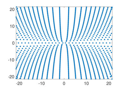
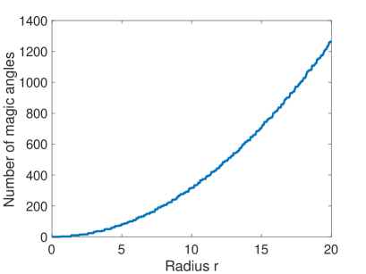
Figure 5. Spectrum of $T_{\mathbf{k}}$ for $\mathbf{k}\notin\Gamma^{*}$ with periodic magnetic field. The magic $\alpha_{1}$ do not depend on the magnetic field strength (left). Number of magic angles within radius $r$ (as in figure on the left) showing quadratic dependence (right), cf. Theorem 6.

Theorem 6 (Magic angles–Periodic magnetic potentials).

Consider the BM model with $\Gamma_{\operatorname{mag}}$-periodic magnetic potential $A\in C^{\infty}({\mathbb{C}}/\Gamma_{\operatorname{mag}};{\mathbb{R}}^{2})$:
Chiral Hamiltonian: The magic angles, and the multiplicity of flat bands of the chiral Hamiltonian (2.2), are independent of the magnetic potential, i.e. $\alpha\in\mathcal{A}_{c}$ for $A=0$ if and only if $\alpha\in\mathcal{A}_{c}$ for non-zero periodic $A\in C^{\infty}({\mathbb{C}}/\Gamma_{\operatorname{mag}};{\mathbb{R}}^{2}).$ In addition the number of magic angles, counting multiplicities, in a disc of radius $R$ satisfies: $|\mathcal{A}_{c}\cap B_{R}(0)|=\mathcal{O}(R^{2}).$
Anti-chiral Hamiltonian: The anti-chiral Hamiltonian (LABEL:eq:achiral), with magnetic potentials as above, does not possess any flat bands at zero, i.e. $\mathcal{A}_{{\operatorname{ac}}}=\emptyset.$ In particular, its spectrum is purely absolutely continuous.

We split the proof of Theorem 6 on the existence/absence of flat bands into two parts, separating the statement about the chiral Hamiltonian from the statement about the anti-chiral Hamiltonian. We start with a discussion of the chiral Hamiltonian.

Proof of Theo. 6, Chiral Hamiltonian:.

For the chiral Hamiltonian, with $\alpha_{0}=0$, it suffices to analyze the nullspaces of the off-diagonal operators (2.2). Without loss of generality, we can study the nullspace of $\mathcal{D}_{\mathbf{k},c}(\alpha_{1})$ where $0\in\operatorname{Spec}(\mathcal{D}_{\mathbf{k},c})(\alpha_{1})\Leftrightarrow\alpha_{1}^{-1}\in\operatorname{Spec}(T_{\mathbf{k}})$ with Birman-Schwinger operator $T_{\mathbf{k}}=(2D_{\bar{z}}-(A_{1}(z)+iA_{2}(z))+\mathbf{k})^{-1}\begin{pmatrix}0&U(z)\\ U_{-}(z)&0\end{pmatrix}$ for $\mathbf{k}\notin\Gamma_{\operatorname{mag}}^{*}.$ For any zero mode $\chi_{\mathbf{k}}\in H^{1}({\mathbb{C}}/\Gamma_{\operatorname{mag}})$ to $D_{\mathbf{k},c}(\alpha_{1},B=0)$ it follows that $\psi_{\mathbf{k}}=\chi_{\mathbf{k}}\cdot e^{-\phi}\in L^{2}({\mathbb{C}}/\Gamma_{\operatorname{mag}})$, with $\phi$ as in the proof of Prop. 4.2 solves for $\mathcal{D}_{\mathbf{k},c}=D_{c}$

$$\mathcal{D}_{\mathbf{k},c}(\alpha_{1})\psi_{\mathbf{k}}=\psi_{0}\underbrace{\mathcal{D}_{\mathbf{k},c}(\alpha_{1},B=0)\chi_{\mathbf{k}}}_{=0}+\chi_{\mathbf{k}}\underbrace{(2D_{\bar{z}}-(A_{1}(z)+iA_{2}(z)))\psi_{0}(z)}_{=0}=0.$$

This shows that $H_{c}(B=0)$ possesses a flat band if and only if $H_{c}(B)$ possesses one, with $B$ induced by a $\Gamma_{\operatorname{mag}}$-periodic magnetic potential $A$. The characterization of magic angles $\alpha_{1}$ as reciprocals of eigenvalues of $T_{\mathbf{k}}$ with $A=0$ follows then from [BEWZ20a, Theo. $2$]. We now utilize the compactness of $T_{\mathbf{k}}$, with $A=0,$ to give an upper bound on the number of magic angles.

Indeed, let $z=x_{1}+ix_{2}=2i\omega(y_{1}+i\omega y_{2})$, we shall first rewrite $D_{\bar{z}}$ and $\mathcal{V}$ in new coordinates $(y_{1},y_{2}).$ Thus, decomposing for $A_{N}:=\Pi_{N}T_{\mathbf{k}},$ with $\Pi_{N}:L^{2}({\mathbb{R}}^{2}/2\pi{\mathbb{Z}}^{2};{\mathbb{C}}^{2})\rightarrow\ell^{2}({\mathbb{Z}}^{2}_{2N+1};{\mathbb{C}}^{2})$ such that $\Pi_{N}\left(\sum_{n\in{\mathbb{Z}}^{2}}a_{\mathbf{n}}e^{i\langle y,\mathbf{n}\rangle}\right)=\{a_{(n_{1},n_{2})}\}_{|n_{j}|\leq N},a_{\mathbf{n}}\in{\mathbb{C}}^{2}$ and introducing $B_{N}:=T_{\mathbf{k}}-A_{N},$ we can estimate, by specializing to $\mathbf{k}=1/2$,

$$\begin{split}\|&A_{N}\|_{1}\leq\|\Pi_{N}(D_{\bar{z}}-\mathbf{k})^{-1}\|_{1}\|\mathcal{V}\|\leq\sqrt{3}\|U\|_{\infty}\sum_{|m|_{\infty}\leq N}\tfrac{1}{\Big{|}\left(m_{1}+\tfrac{1}{2}\right)^{2}+\left(m_{1}+\tfrac{1}{2}\right)\left(m_{2}+\tfrac{1}{2}\right)+\left(m_{2}+\tfrac{1}{2}\right)^{2}\Big{|}^{1/2}}\\ &=\sqrt{3}\|U\|_{\infty}\Bigg{(}\sum_{|m|_{\infty}\leq 2}\Big{|}\left(m_{1}+\tfrac{1}{2}\right)^{2}+\left(m_{1}+\tfrac{1}{2}\right)\left(m_{2}+\tfrac{1}{2}\right)+\left(m_{2}+\tfrac{1}{2}\right)^{2}\Big{|}^{-1/2}\\ &\quad+\sum_{2<|m|_{\infty}\leq N}\Big{|}\left(m_{1}+\tfrac{1}{2}\right)^{2}+\left(m_{1}+\tfrac{1}{2}\right)\left(m_{2}+\tfrac{1}{2}\right)+\left(m_{2}+\tfrac{1}{2}\right)^{2}\Big{|}^{-1/2}\Bigg{)}\\ &\leq\sqrt{3}\|U\|_{\infty}\left(17+\int_{1/2}^{\sqrt{2}N}\int_{0}^{2\pi}\tfrac{1}{\sqrt{1+\frac{1}{2}\sin(2\varphi)}}\ d\varphi\right)=\sqrt{3}\|U\|_{\infty}\left(17+(\sqrt{2}N-\tfrac{1}{2})7\right)\leq C_{2}N.\end{split}$$

Similarly, we have that

$$\|B_{N}\|\leq\sup_{|m|_{\infty}>N}\Big{|}\left(m_{1}+\tfrac{1}{2}\right)^{2}+\left(m_{1}+\tfrac{1}{2}\right)\left(m_{2}+\tfrac{1}{2}\right)+\left(m_{2}+\tfrac{1}{2}\right)^{2}\Big{|}^{-1/2}\|U\|_{\infty}\leq\frac{\|U\|_{\infty}}{(N-\tfrac{1}{2})}\leq\frac{C_{1}}{N}.$$

Thus, for $|\alpha_{1}|\leq R$ we take $N$, large enough, such that $\|\alpha_{1}B_{N}\|\leq\frac{RC_{1}}{N}<1/2.$ Thus, we may pick $N=\lceil RC_{1}/2\rceil.$ Hence, we can write $1-\alpha_{1}T_{\mathbf{k}}=(1-\alpha_{1}B_{N})(1-(1-\alpha_{1}B_{N})^{-1}\alpha_{1}A_{N})$ and the magic $\alpha_{1}$’s are the zeros of $f(z)=\det(1-(1-\alpha_{1}B_{N})^{-1}\alpha_{1}A_{N}).$ Using the standard bound for Fredholm determinants, we have $|f(z)|\leq e^{2R\|A_{N}\|_{1}}\leq e^{2RC_{2}N}\leq e^{R^{2}C_{1}C_{2}}.$ Hence, as $f(0)=1$, Jensen’s formula implies that the number $n$ of zeros of $f$ for $\alpha\in B_{0}(R)$ is bounded by $n(R)\leq\log(2)^{-1}\Big{(}4R^{2}C_{1}C_{2}\Big{)}.$ ∎

We now continue by showing that the anti-chiral Hamiltonian does not possess flat bands at energy zero.

Proof of Theo.6, Anti-Chiral Hamiltonian:.

It is well-known that the singular continuous spectrum for periodic operators of this type is empty. Thus, it suffices to exclude embedded point spectrum. The existence of an embedded eigenvalue implies by Bloch-Floquet theory that there is an open set $\Omega$ such that for all $\mathbf{k}\in\Omega$ we have $0\in\operatorname{Spec}(\mathcal{K}_{\mathbf{k}}(\alpha_{0}))$ where

$$\mathcal{K}_{\mathbf{k}}(\alpha_{0}):=\begin{pmatrix}\lambda&Q_{\mathbf{k}}(\alpha_{0})\\ Q_{\mathbf{k}}(\alpha_{0})^{*}&\lambda\end{pmatrix}\text{ with }Q_{\mathbf{k}}(\alpha_{0}):=\begin{pmatrix}\alpha_{0}e^{-i\theta/2}V(z)&\mathscr{D}_{z}(\overline{\mathbf{k}},A)\\ \mathscr{D}_{\bar{z}}(\mathbf{k},A)&\alpha_{0}e^{-i\theta/2}\overline{V(z)}\end{pmatrix}$$

and we introduced

$$\begin{split}\mathscr{D}_{z}(\mathbf{\bar{k}},A)=2D_{z}+\mathbf{\bar{k}}-(A_{1}(z)-iA_{2}(z))\text{ and }\mathscr{D}_{\bar{z}}(\mathbf{k},A)=2D_{\bar{z}}+\mathbf{k}-(A_{1}(z)+iA_{2}(z)).\end{split}$$ (5.2)

Since the operator $\mathcal{K}_{\mathbf{k}}$ depends analytically on the real and imaginary part of $\mathbf{k}$ individually, the existence of an embedded eigenvalue implies that the entire band would be flat. This can be easily seen by looking at all possible rays of $\mathbf{k}$ in $\Omega.$

We shall omit the $\alpha_{0}$ dependence and set $\theta=0$ to simplify notation. The formal inverse of $\mathcal{K}_{\mathbf{k}}$ is given by $\mathcal{K}_{\mathbf{k}}^{-1}=\begin{pmatrix}\lambda(\lambda^{2}-Q_{\mathbf{k}}Q_{\mathbf{k}}^{*})^{-1}&-Q_{\mathbf{k}}(\lambda^{2}-Q_{\mathbf{k}}^{*}Q_{\mathbf{k}})^{-1}\\ -(\lambda^{2}-Q_{\mathbf{k}}^{*}Q_{\mathbf{k}})^{-1}Q_{\mathbf{k}}^{*}&\lambda(\lambda^{2}-Q_{\mathbf{k}}^{*}Q_{\mathbf{k}})^{-1}\end{pmatrix}.$ The operator ${\mathbb{R}}\ni\mathbf{k}_{1}\mapsto\mathcal{K}_{\mathbf{k}}$ for $\mathbf{k}_{2}$ fixed, and $\lambda\in{\mathbb{R}}$ is a self-adjoint holomorphic family with compact resolvent on $L^{2}(\mathbb{C}/\Gamma)$. A flat band would imply that $\mathcal{K}_{\mathbf{k}}(\alpha_{0})$ is not invertible for any $\mathbf{k}\in{\mathbb{C}}.$ To simplify the analysis, we write

$$\begin{split}Q_{\mathbf{k}}&=\underbrace{\sum_{j=1}^{2}(D_{j}+\mathbf{k}_{j}-A_{j}(x))\sigma_{j}}_{=:{H}_{\text{D},\mathbf{k}}}+\mathcal{V}\text{ and }Q_{\mathbf{k}}^{*}=\underbrace{\sum_{j=1}^{2}(D_{j}+\mathbf{k}_{j}-A_{j}(x))\sigma_{j}}_{=:{H}_{\text{D},\mathbf{k}}}+\overline{\mathcal{V}},\end{split}$$ (5.3)

where $\mathcal{V}=\operatorname{diag}(V,\overline{V}).$ Recall also the Pauli operator ${H}_{\text{P},\mathbf{k}}$ given as

$$\begin{split}{H}_{\text{P},\mathbf{k}}=({H}_{\text{D},\mathbf{k}})^{2}=&\left((D_{1}+\mathbf{k}_{1}-A_{1}(x))^{2}+(D_{2}+\mathbf{k}_{2}-A_{2}(x))^{2}\right)-(\partial_{1}A_{2}-\partial_{2}A_{1})(x)\sigma_{3}.\end{split}$$ (5.4)

In this setting, we have that both $\mathbf{k}_{1},\mathbf{k}_{2}$ are real. Thus, we have for $S(\lambda)={H}_{\text{P},\mathbf{k}}-\lambda^{2}$

$$\begin{split}Q_{\mathbf{k}}^{*}Q_{\mathbf{k}}-\lambda^{2}&=(1+\underbrace{([Q_{\mathbf{k}}^{*},\mathcal{V}]+\mathcal{V}Q_{\mathbf{k}}^{*}+\mathcal{V}^{*}Q_{\mathbf{k}}+\mathcal{V}\mathcal{V}^{*})S(\lambda)^{-1}}_{=:W_{1}(\lambda)})S(\lambda)\\ Q_{\mathbf{k}}Q_{\mathbf{k}}^{*}-\lambda^{2}&=(1+\underbrace{([Q_{\mathbf{k}},\mathcal{V}^{*}]+\mathcal{V}^{*}Q_{\mathbf{k}}+\mathcal{V}Q_{\mathbf{k}}^{*}+\mathcal{V}\mathcal{V}^{*})S(\lambda)^{-1}}_{=:W_{2}(\lambda)})S(\lambda).\end{split}$$ (5.5)

We now complexify the real part of $\mathbf{k}$, which is $\mathbf{k}_{1}$, and choose $\mathbf{k}=\mathbf{k}_{1}+i\mathbf{k}_{2}$ with $\mathbf{k}_{1}:=(\mu+iy)$, where $\mu,y,\mathbf{k}_{2}\in{\mathbb{R}}.$ Since the principal symbol of $Q_{\mathbf{k}}$ is the Dirac operator and the Pauli operator its square, we find by self-adjointness that $\|S(\lambda)^{-1}\|,\|Q_{\mathbf{k}}S(\lambda)^{-1}\|,\|Q_{\mathbf{k}}^{*}S(\lambda)^{-1}\|=\mathcal{O}(|y|^{-1}).$

Assuming that there exists a flat band to $\mathcal{K}_{\mathbf{k}}$, it follows that $-1\in\operatorname{Spec}(W_{1}(\lambda))\cap\operatorname{Spec}(W_{2}(\lambda))$ in a complex neighbourhood of $\mathbf{k}_{1}\in{\mathbb{R}}$ by Rellich’s theorem. Then [Ka, Thm $1.9$] implies that for all $\mathbf{k}_{1}\in{\mathbb{C}}$ we have $-1\in\operatorname{Spec}(W_{1}(\lambda))\cap\operatorname{Spec}(W_{2}(\lambda)).$ But this is impossible, by the estimates on $\|S(\lambda)^{-1}\|$ for $|y|$ large enough. ∎

For general magnetic fields, the concept of bands does not apply. Instead, since a flat band for a Floquet operator, corresponds to an eigenvalue of infinite multiplicity of the original operator, one should study such eigenvalues of infinite multiplicity. Then, we have the following result that we split up into one statement on flat bands and one on eigenvalues of infinite multiplicity

Figure 6. Periodic magnetic field $A_{1}(z)=2\sqrt{3}\cos(\operatorname{Im}(z))$: On the left, the lowest bands of the anti-chiral Hamiltonian, $\alpha_{0}=1$, where $0$ is not protected, under periodic magnetic perturbations, on the right the lowest bands of the chiral Hamiltonian, $\alpha_{1}=1$, where $0$ is protected in the spectrum.

Theorem 7 (Eigenvalues).

Let $\alpha_{1}\in\mathcal{A}$ be a magic angle. When adding to $H_{c}(B=0)$ any magnetic field $B\in L^{\infty}_{\operatorname{comp}}$ with flux $\lfloor\Phi/2\pi\rfloor\geq 1$ or any periodic magnetic potential $A_{\operatorname{per}}\in C^{\infty}(E),$ the operator $H_{c}(B)$ has an eigenvalue of infinite multiplicity at $0$. If $\alpha_{1}$ is not magic, and $B\in L^{\infty}_{\operatorname{comp}}$ as above, then $H_{c}$ possesses an eigenvalue of multiplicity $\lfloor\Phi/2\pi\rfloor$ at zero. In particular, for non-zero constant magnetic fields the chiral Hamiltonian possesses an eigenvalue of infinite multiplicity at zero for any $\alpha_{1}\in\mathbb{R}.$

Proof.

To see that $0$ is in the spectrum of the chiral magnetic Hamiltonian, we use that we can multiply any $\psi=(\psi_{1},0)\in{\mathbb{C}}^{4}$, with $D_{c}(B=0)\psi_{1}=0$ by a $\varphi_{1}$, satisfying $(2D_{\bar{z}}-A(z))\varphi_{1}=0,$ to define the new function $\chi=(\varphi_{1}\psi_{1},0)$ which then satisfies $H_{c}(B)\chi=0.$ While there also exists a solution $D_{c}(B=0)^{*}\psi_{2}=0$, there does not exist a zero mode to the operator $2D_{z}-\overline{A(z)}$ for $B>0.$

By the Aharonov-Casher effect [CFKS, Sec.$6.4$], there are precisely $\lfloor\Phi/(2\pi)\rfloor$ linearly independent square-integrable zero modes $\varphi_{1},...,\varphi_{\lfloor\Phi/(2\pi)\rfloor}$. Multiplying this with the Floquet-periodic zero modes of the chiral model $\psi$, which exist for all $\alpha_{1}\in\mathbb{C}$, this gives the claim for the magnetic fields of compact support. When $\alpha_{1}$ is magic, the non-magnetic Hamiltonian exhibits an eigenvalue of infinite multiplicity at energy zero. Thus, there exists a countable family of zero modes $(\psi_{n})_{n}$ to $D_{c}(B=0)$ at $\alpha_{1}$ magic. Thus, we can construct a countable family of zero modes $\chi_{n}:=\varphi_{1}\psi_{n}$ to $D_{c}(B)$ at $\alpha_{1}$ magic.

Turning to constant magnetic fields with flux $\Phi\in 2\pi\mathbb{Q}$, through a fundamental domain $E$ for some $n$, then by adding potentials $A_{\operatorname{per}}\in C^{\infty}(E)$, there is by Proposition 4.2 a $\varphi_{\mathbf{k}}$ such that $(a_{k}+A_{\operatorname{per}})\varphi_{\mathbf{k}}=0$ and the existence of a flat band at zero follows. If the fields are not commensurable, the same argument shows the existence of an eigenvalue of infinite multiplicity.

The stability under perturbations by periodic magnetic potentials, follows directly from the existence of periodic $\psi_{0}\neq 0$ such that, $(2D_{\bar{z}}+A_{\operatorname{per}})\psi_{0}=0.$ ∎

6. Hörmander condition and exponential localization of bands

In this section, we study the exponential squeezing of bands for periodic magnetic fields and small angles. In particular, we shall see that in the chiral model, there will be at least $\sim 1/\theta$ many bands in an exponentially (in $\theta$) small neighbourhood around zero. We deduce this property by studying the existence of localized quasi-modes in phase space. Phrased differently, for small twisting angles any angle wants to be magic. We shall prove this for the chiral model and then show that in the anti-chiral model such quasi-modes do not exist. In the case of the non-magnetic BM Hamiltonian, this has been established in [BEWZ20a, BEWZ20b].

6.1. Exponential squeezing in chiral model

The chiral model possesses in general a lot quasi-modes located close to the zero energy level. Indeed, since $h=1/B$ is our semiclassical parameter, the principal symbol of $hD_{c}^{\theta}$, with $D_{c}^{\theta}$ as in (2.2), is just $p(z,\zeta):=\sigma_{0}(hD_{c}^{\theta})(z,\zeta)=2\bar{\zeta}-A(z)$. The existence of localized modes will depend on the vanishing/non-vanishing of the bracket

$$\{p,\bar{p}\}(z)=2(\partial_{z}A(z)-\partial_{\bar{z}}\overline{A(z)})=2iB(z).$$ (6.1)

We observe that with our quantization, the principal symbol and consequently the Poisson bracket are independent of the potentials. To see the effect of the potentials, one may look at the non-equivalent tight-binding limit

$$\mathcal{D}_{c,\text{TB}}^{\theta}=\begin{pmatrix}2\theta D_{\bar{z}}-A(z)&U(z)\\ U_{-}(z)&2\theta D_{\bar{z}}-A(z)\end{pmatrix}.$$ (6.2)

The semiclassical principal symbol of $\mathcal{D}_{c,\text{TB}}^{\theta}$ is given by

$$\sigma_{0}(\mathcal{D}_{c,\text{TB}}^{\theta})(z,\zeta)=\begin{pmatrix}2\bar{\zeta}-A(z)&U(z)\\ U_{-}(z)&2\bar{\zeta}-A(z)\end{pmatrix}.$$

The determinant of the principal symbol of $\mathcal{D}_{c,\text{TB}}^{\theta}$ and its conjugate symbol is given for $W(z):=U(z)U_{-}(z)$ by $q(z,\zeta):=\left(2\bar{\zeta}-A(z)\right)^{2}-W(z).$

We then have the following existence of quasimodes result, which for the semiclassical scaling in $\mathcal{D}_{c}^{\theta}$ follows from the Poisson-bracket (6.1) along the lines as presented for $\mathcal{D}_{c,\text{TB}}^{\theta}$ below.

Proposition 6.1.

There exists an open set $\Omega\subset\mathbb{C}$ and a constant $c$ such that for any $\mathbf{k}\in\mathbb{C}$ and $z_{0}\in\Omega$, there exists a family $\theta\mapsto\mathbf{u}_{\theta}\in C^{\infty}(\mathbb{C}/\Gamma;\mathbb{C}^{2})$ such that for $0<\theta<\theta_{0}$,

$$|(\mathcal{D}_{c,\text{TB}}^{\theta}-\theta\mathbf{k})\mathbf{u}_{\theta}(z)|\leq e^{-c/\theta},\quad\|\mathbf{u}_{\theta}\|_{L^{2}}=1,\quad|\mathbf{u}_{\theta}(z)|\leq e^{-c|z-z_{0}|^{2}/\theta}.$$ (6.3)

Proof.

Since the Poisson-bracket in complex coordinates reads

$$\begin{split}\{q_{1},q_{2}\}=\partial_{\zeta}q_{1}\partial_{z}q_{2}+\partial_{\bar{\zeta}}q_{1}\partial_{\bar{z}}q_{2}-\partial_{z}q_{1}\partial_{\zeta}q_{2}-\partial_{\bar{z}}q_{1}\partial_{\bar{\zeta}}q_{2},\end{split}$$ (6.4)

we find that under the constraint that $q=\bar{q}=0$ at some point $(z,\zeta)$

$$\begin{split}\{q,\bar{q}\}(z,\zeta)&=(\partial_{\bar{\zeta}}q\partial_{\bar{z}}\bar{q}-\partial_{z}q\partial_{\zeta}\bar{q})(z,\zeta)=8i|W(z)|B(z)-8i\operatorname{Im}(\partial_{z}W(z)\overline{W(z)}^{1/2}).\end{split}$$ (6.5)

We then have that using that $U(z)=0$

$$W(z)=-z^{2}(\partial_{z}U(0))^{2}(1+\mathcal{O}(|z|))\text{ and }\partial_{z}W(z)=-2z(\partial_{z}U(0))^{2}(1+\mathcal{O}(|z|)),$$

which shows that

$$\overline{W(z)}^{1/2}\partial_{z}W(z)=2i|z|^{2}|\partial_{z}U(0)|^{2}\partial_{z}U(0)(1+\mathcal{O}(|z|)).$$

This implies the following expansion of the Poisson bracket at zero

$$\{q,\bar{q}\}=8i|z|^{2}|\partial_{z}U(0)|^{2}(B(z)-2\operatorname{Re}(\partial_{z}U(0)))(1+\mathcal{O}(|z|)).$$

The result then follows from a real-analytic version [DSZ04, Theorem 1.2] of Hörmander’s local solvability condition: For a differential operator $Q=\sum_{|\alpha|\leq m}a_{\alpha}(x,\theta)(\theta D)^{\alpha}$ with real-analytic maps $x\mapsto a_{\alpha}(x,\theta)$ near some $x_{0}$, we let $q(x,\xi)$ be the semiclassical principal symbol of $Q$. If for phase space coordinates $(x_{0},\xi_{0})$ we have $q(x_{0},\xi_{0})=0,\ \ \{q,\bar{q}\}(x_{0},\xi_{0})\neq 0,$ then there exists a family $v_{\theta}\in C^{\infty}_{\rm{c}}(\Omega)$, $\Omega$ is a neighbourhood of $x_{0}$, such that for some $c>0$

$$|(\theta D)^{\alpha}_{x}Qv_{\theta}(x)|\leq C_{\alpha}e^{-c/\theta},\ \ \|v_{\theta}\|_{L^{2}}=1,\ \ |(\theta\partial_{x})^{\alpha}v_{\theta}(x)|\leq C_{\alpha}e^{-c|x-x_{0}|^{2}/\theta}.$$ (6.6)

∎

We then have the following result exhibiting the exponential squeezing of bands:

Theorem 8 (Exponential squeezing of bands).

Consider the semiclassical scaling of the chiral Hamiltonian with magnetic potential $A\in C^{\infty}(E)$ inducing a non-zero magnetic field or consider the chiral Hamiltonian with tight-binding scaling (6.2) and arbitrary magnetic potential $A\in C^{\infty}(E)$. For the Floquet-transformed operator, the spectrum is a union of bands

$$\operatorname{Spec}_{L^{2}(E)}(H_{\mathbf{k}}^{\theta})=\{E_{j}(\mathbf{k},\theta)\}_{j\in{\mathbb{Z}}},E_{j}(\mathbf{k},\theta)\leq E_{j+1}(\mathbf{k},\theta),\mathbf{k}\in{\mathbb{C}},$$

where $E_{0}(\mathbf{k},\theta)=\min_{j}|E_{j}(\mathbf{k},\theta)|.$ Then there exist constants $c_{0},c_{1},c_{2}>0$ and $\theta_{0}>0$ such that for all $\mathbf{k}\in{\mathbb{C}}$ and $\theta\in(0,\theta_{0})$,

$$|E_{j}(\mathbf{k},\theta)|\leq c_{0}e^{-c_{1}/\theta},|j|\leq c_{2}\theta^{-1}.$$

Proof.

By using the above proposition and [BEWZ20a, Prop. $4.2$], we can use the proof of [BEWZ20a, Theo. $5$] to deduce the result. ∎

6.2. Anti-chiral model

To see that the conclusion of Theorem 8 does not hold for the anti-chiral Hamiltonian, we proceed as follows, and shall again restrict us to the slightly more technical tight-binding scaling. Consider in (LABEL:eq:achiral) for small $\theta>0$ the operator, with $b_{\mathbf{k}}:=2\theta D_{z}-\overline{A(z)}-\theta\overline{\mathbf{k}}$,

$$\mathcal{D}_{{\operatorname{ac}},\text{TB}}^{\theta}=\begin{pmatrix}V&b_{\mathbf{k}}\\ b_{\mathbf{k}}^{*}&\overline{V}\end{pmatrix}.$$

Then, the existence of a zero mode is equivalent, for $z\in\Omega:=\{w\in{\mathbb{C}};V(w,\bar{w})\neq 0\}$, to a zero mode of the operator

$$P(\theta)v_{\theta}(z)=\left(V(z)b^{*}_{\mathbf{k}}(V(z)^{-1}b_{\mathbf{k}}-|V(z)|^{2}\right)v_{\theta}(z).$$

We then find

Proposition 6.2.

If $u(\theta)$ is smooth on a bounded domain with $\operatorname{WF}_{h}(u(\theta))=\{(z_{0},\zeta_{0})\}\in T^{*}\Omega,$ then it follows that $\|u(\theta)\|\leq\frac{C}{\theta}\|P(\theta)u(\theta)\|,\theta\downarrow 0.$ Thus, there do not exist any quasi-modes $P(\theta)u(\theta)=\mathcal{O}(\theta^{\infty}).$

Proof.

Since $\sigma_{0}(p)$ is real-valued, the condition $\partial p\neq 0\text{ on }\{p=0\}$ precisely means that $p$ is of real principal type which implies the result by [Zw12, Theo. $12.4$]. ∎

The principal symbol of $P(\theta)$ is given by $\sigma_{0}(P(\theta))(z,\bar{z},\zeta,\bar{\zeta})=|2\zeta-(A_{1}-iA_{2})|^{2}-\alpha_{0}^{2}|V(z,\bar{z})|^{2}.$ This is of real principal type since real valued and $\sigma_{0}(P(\theta))=0$ implies $\partial_{\zeta}\sigma_{0}(P(\theta))=4(2\bar{\zeta}-(A_{1}+iA_{2}))\neq 0$ assuming $V(z,\bar{z})\neq 0$ for all $z\in\mathbb{C}$. By the proposition above, $\|P(\theta)u(\theta)\|$ is bounded below by function of order $\theta$. In particular, (6.3) does not hold.

6.3. Landau levels in the absence of a magnetic field

In the preceding subsection, we showed that for small angles there is an abundance of almost flat bands at small twisting angles close to zero energy. In this subsection, we try to address the question: Do similar quasimodes exist at non-zero energy levels?

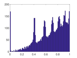
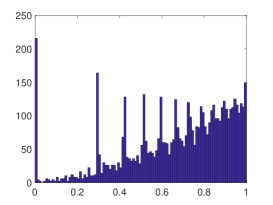
Figure 7. Histogram of Bloch eigenvalues (x-axis Energy/$\sqrt{3}$, y-axis Abundance) of chiral Hamiltonian for fixed $k=1/2$ and $h=0.03$, $h=0.01$, and $h=0.005$, respectively in the absence of magnetic fields. The Landau levels are clearly visible with the one at zero energy most significantly pronounced.

It has been proposed, in the absence of external magnetic or electric fields, that there is a close connection between electromagnetic Dirac operators and the chiral/anti-chiral models. Recall that in the chiral limit, we need to consider, in the semiclassical limit $h$, which is closely connected to the study of small twisting angles, the off-diagonal block operator

$$D=\begin{pmatrix}2hD_{\bar{z}}-A(z)&U(z)\\ U(-z)&2hD_{\bar{z}}-A(z)\end{pmatrix}.$$

By conjugating $D$ with $\mathscr{U}=\frac{1}{\sqrt{2}}\begin{pmatrix}i&1\\ -i&1\end{pmatrix}$, we yield a matrix,

$$\mathcal{D}(z,hD_{\bar{z}})=\mathscr{U}D\mathscr{U}^{*}=\begin{pmatrix}D_{h}^{A}(z)+\frac{i}{2}(U(z)-U(-z))&\frac{i}{2}(U(z)+U(-z))\\ -\frac{i}{2}(U(z)+U(-z))&D_{h}^{A}(z)-\frac{i}{2}(U(z)-U(-z))\end{pmatrix},$$

where $D_{h}^{A}(z)=2hD_{\bar{z}}-A(z)$. Here $U(z)-U(-z)=2i\sum\limits_{k=0}^{2}\omega^{k}\sin(\operatorname{Im}(z\bar{\omega}^{k}))=3z-\frac{3z\bar{z}^{2}}{8}+\mathcal{O}(|z|^{5})$ has a Taylor expansion containing only odd products of $z^{n_{1}}\bar{z}^{n_{2}}$, $n_{1}+n_{2}\in 2\mathbb{N}_{0}+1$. Similarly, $U(z)+U(-z)=2\sum_{k=0}^{2}\omega^{k}\cos(\operatorname{Im}(z\bar{\omega}^{k}))=\frac{3}{4}\bar{z}^{2}+\mathcal{O}(|z|^{4})$ has a Taylor expansion containing only even products of $z^{n_{1}}\bar{z}^{n_{2}}$, $n_{1}+n_{2}\in 2\mathbb{N}.$ By a simple change of variables in $\mathcal{D}$, $z\mapsto\sqrt{h}z$, we find in terms of $W_{1}(z)=\tfrac{i}{2}(U(\sqrt{h}z)-U(-\sqrt{h}z))$ and $W_{2}(z)=\tfrac{i}{2}(U(\sqrt{h}z)+U(-\sqrt{h}z))$

$$D(\sqrt{h}z,\sqrt{h}D_{\bar{z}})=\begin{pmatrix}D_{\sqrt{h}}^{A}(\sqrt{h}z)+W_{1}(z)&W_{2}(z)\\ -W_{2}(z)&D_{\sqrt{h}}^{A}(\sqrt{h}z)-W_{1}(z)\end{pmatrix}.$$

$$\begin{split}P&=\operatorname{diag}(D(\sqrt{h}z,\sqrt{h}D_{\bar{z}})^{*}D(\sqrt{h}z,\sqrt{h}D_{\bar{z}}),D(\sqrt{h}z,\sqrt{h}D_{\bar{z}})D(\sqrt{h}z,\sqrt{h}D_{\bar{z}})^{*}).\end{split}$$

This operator is a block-diagonal $4\times 4$ matrix where the first $2\times 2$ block $P_{2}:=\begin{pmatrix}P_{2,11}&P_{2,12}\\ P_{2,12}^{*}&P_{2,22}\end{pmatrix}$ is given by

$$\begin{split}P_{2,11}&=(D_{\sqrt{h}}^{A}(\sqrt{h}z)+W_{1})(D_{\sqrt{h}}^{A}(\sqrt{h}z)^{*}+\overline{W_{1}})+|W_{2}|^{2},\\ P_{2,12}&=-(D_{\sqrt{h}}^{A}(\sqrt{h}z)+W_{1})\overline{W_{2}}+W_{2}(D_{\sqrt{h}}^{A}(\sqrt{h}z)^{*}-\overline{W_{1}}),\text{ and }\\ P_{2,22}&=(D_{\sqrt{h}}^{A}(\sqrt{h}z)-W_{1})(D_{\sqrt{h}}^{A}(\sqrt{h}z)^{*}-\overline{W_{1}})+|W_{2}|^{2}.\end{split}$$

The leading order expansion in $h$ suggests that the low-lying spectrum of $P$ is determined by the leading-order expansion

$$P\varphi=\operatorname{diag}(P_{1}^{\text{lin}},P_{2}^{\text{lin}})\varphi+\mathcal{O}_{\varphi}(h^{2}),$$

valid for any fixed Schwartz-function $\varphi\in\mathscr{S}(\mathbb{C})$, with

$$P_{1}^{\text{lin}}=h\operatorname{diag}(a_{B}a_{B}^{*},b_{B}b_{B}^{*})\text{ and }P_{2}^{\text{lin}}=h\operatorname{diag}(a_{B}^{*}a_{B},b_{B}^{*}b_{B})$$

where

$$a_{B}=2D_{z}-\frac{(3-B_{0})i}{2}\bar{z}\text{ and }b_{B}=2D_{z}-\frac{(3+B_{0})i}{2}.$$

In particular, the two components satisfy the commutation relations

$$[a_{B},a_{B}^{*}]=(6-2B_{0})=2B_{a}\text{ and }[b_{B}^{*},b_{B}]=(6+2B_{0})=2B_{b}.$$

Here, we introduced $B_{a}:=(3-B_{0})$ and $B_{b}:=(3+B_{0}).$ Analogously, for the original Hamiltonian, we already find the leading order in $\sqrt{h}$

$$H^{\operatorname{lin}}(\sqrt{h}z,\sqrt{h}D_{\bar{z}})=\sqrt{h}\begin{pmatrix}0_{\mathbb{C}^{2\times 2}}&\operatorname{diag}(a_{B},b_{B})\\ \operatorname{diag}(a_{B},b_{B})^{*}&0_{\mathbb{C}^{2\times 2}}\end{pmatrix}.$$

Proposition 6.3.

Let $B_{a},B_{b}\neq 0$, then the spectrum of $H^{\operatorname{lin}}$ consists of infinitely degenerate eigenvalues

$$\operatorname{Spec}(H^{\text{lin}})=\{\operatorname{sgn}(n_{1})\sqrt{2|n_{1}|B_{a}},\operatorname{sgn}(n_{2})\sqrt{2|n_{2}|B_{b}},\text{ with }n\in\mathbb{Z}^{2}\}.$$

In particular, to each eigenvalue one can find a dense set of exponentially localized Schwartz functions.

Proof.

We start by studying the squared operator

Let $U_{\operatorname{FW}}:=\frac{1}{\sqrt{2}}(1+\sigma_{3}\operatorname{sgn}(P^{\operatorname{lin}}))$ be the Foldy-Wouthuysen transform then

$$U_{\operatorname{FW}}H^{\text{lin}}U_{\operatorname{FW}}^{*}=\sqrt{h}\operatorname{diag}(\sqrt{a_{B}a_{B}^{*}},\sqrt{b_{B}b_{B}^{*}},-\sqrt{a_{B}^{*}a_{B}},-\sqrt{b_{B}^{*}b_{B}}).$$

We assume in the sequel that $B_{a}>0$ and/or $B_{b}>0$ where at least one of the two conditions is satisfied for every $B_{0}$

$$\begin{split}\operatorname{Spec}(a_{B}^{*}a_{B})\subset\{0,2B_{a},4B_{a},...\}\text{ and }\operatorname{Spec}(a_{B}a_{B}^{*})\subset\{2B_{a},4B_{a},...\},\\ \operatorname{Spec}(b_{B}^{*}b_{B})\subset\{0,2B_{b},4B_{b},...\}\text{ and }\operatorname{Spec}(b_{B}b_{B}^{*})\subset\{2B_{b},4B_{b},...\}.\end{split}$$ (6.7)

The ground state solutions, in the case $B_{i}>0$, are infinitely degenerate and then given by

$$\psi_{0}^{m_{j}}(z)=e^{-\frac{B_{i}}{4}|z|^{2}}z^{m_{j}-1/2},\text{ with }m_{j}\in\mathbb{N}_{0}+1/2.$$

Here, $m_{j}$ is the eigenvalue of the associated angular momentum operator orthogonal to the plane. The commutation relations can be used to generate higher Landau levels from the zero modes and show the converse inclusion in (6.7). The explicit form of the higher Landau levels can be found for exampled in [RB17]. ∎

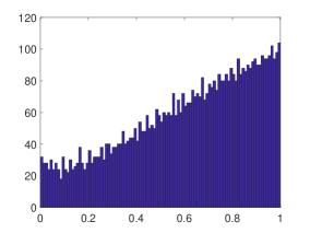
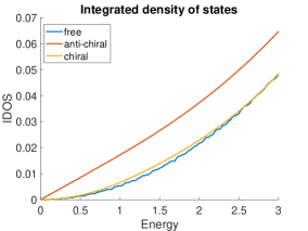
Figure 8. Histogram of anti-chiral model and full Hamiltonian with $h=0.01.$

Appendix A Special functions

Let $\Lambda$ be a $2d$ lattice on ${\mathbb{C}}$. The Weierstraß $\wp$ function is an elliptic function defined by

$$\wp(z,\Lambda):=\frac{1}{z^{2}}+\sum_{\gamma\in\Lambda\setminus\{0\}}\left(\frac{1}{(z-\gamma)^{2}}-\frac{1}{\gamma^{2}}\right).$$

It is the negative derivative of the Weierstraß $\zeta$-function

$$\zeta(z,\Lambda)=\frac{1}{z}+\sum_{\gamma\in\Lambda\setminus\{0\}}\Big{(}\frac{1}{z-\gamma}+\frac{1}{\gamma}+\frac{z}{\gamma^{2}}\Big{)},\quad\text{i.e.}\quad\wp(z,\Lambda)=\zeta(z,\Lambda)^{\prime}.$$

The Weierstraß $\zeta$-function is further the logarithm derivative of Weierstraß sigma function

$$\tilde{\sigma}(z,\Lambda)=z\prod_{\gamma\in\Lambda\setminus\{0\}}\Big{(}1-\frac{z}{\gamma}\Big{)}e^{\frac{z}{\gamma}+\frac{z^{2}}{2\gamma^{2}}},\quad\text{i.e.}\quad\zeta(z,\Lambda)=\frac{d}{dz}\log(\tilde{\sigma}(z,\Lambda))=\frac{\tilde{\sigma}^{\prime}(z,\Lambda)}{\tilde{\sigma}(z,\Lambda)}.$$

We shall now specialize to $\Gamma_{\lambda}$ and discuss when does $\tilde{\sigma}$ coincide with $\sigma$. If $\lambda_{1}=\lambda_{2}$, the symmetries of $\Gamma$ imply that

$$\tilde{\sigma}(\omega z)=\omega\tilde{\sigma}(z)\text{ and }\overline{\tilde{\sigma}(z)}=\tilde{\sigma}(\bar{z}).$$

Hence, using the previous relation, we find that

$$\zeta(\omega z)=\bar{\omega}\zeta(z)\text{ and }\overline{\zeta(z)}=\zeta(\bar{z}).$$

Defining then

$$\eta_{1}:=\frac{\zeta(z+v_{1})-\zeta(z)}{2}\text{ and }\eta_{2}:=\frac{\zeta(z+v_{2})-\zeta(z)}{2}.$$

We find by setting $z=-v_{1}/2$ and $z=-v_{2}/2$, respectively, since $\zeta$ is an odd function,

$$\eta_{1}=\zeta(v_{1}/2)\text{ and }\eta_{2}=\zeta(v_{2}/2)=\bar{\omega}\zeta(v_{1}/2).$$

Then by Legendre’s relation [H18, (14)]

$$\eta_{1}v_{2}-v_{1}\eta_{2}=\zeta(v_{1}/2)(v_{2}-\bar{\omega}v_{1})=\pi i,$$

we find that

$$\eta_{1}=-\frac{3}{8\lambda_{1}}+i\frac{\sqrt{3}}{8\lambda_{1}}=\frac{\pi\bar{v_{1}}}{2A}\text{ and }\eta_{2}=\frac{3}{8\lambda_{1}}+i\frac{\sqrt{3}}{8\lambda_{1}}=\frac{\pi\bar{v_{2}}}{2A}.$$

Here $A=\frac{\lambda_{1}^{2}8\pi^{2}}{3\sqrt{3}}$ is the area of the fundamental domain. Comparing with [H18, (17)], we see that the modular-invariant and regular Weierstaß sigma function coincide.

For lattice vectors $v_{1},v_{2}$ the Weierstaß sigma function can then be efficiently implemented numerically using

$$\sigma(z)=v_{1}e^{\eta_{1}z^{2}/v_{1}}\frac{\theta_{1}(\pi z/v_{1}|\omega)}{\pi\theta_{1}^{\prime}(0|\omega)}=v_{1}e^{\eta_{1}z^{2}/v_{1}}\frac{\theta_{1}(\pi z/v_{1}|\omega)}{\pi\theta_{1}^{\prime}(0|\omega)},$$ (A.1)

where

$$\theta_{1}(z|\tau)=\sum_{n\in{\mathbb{Z}}}e^{\pi in^{2}\tau+2\pi inz}\text{ for }\operatorname{Im}(\tau)>0.$$

For the honeycomb lattice, this is

$$\sigma(z)\propto e^{\frac{3\sqrt{3}}{16\pi\lambda_{1}^{2}}z^{2}}\theta_{1}(z/(4i\omega\lambda_{1})|\omega).$$

References

- [AvSi] J. Avron, B. Simon, Stability of gaps for periodic potentials under variation of a magnetic field, J. Phys. A: Math. Gen. 18, (1985) 2199-2205.
- [BEWZ20a] S. Becker, M. Embree, J. Wittsten and M. Zworski, Mathematics of magic angles in a model of twisted bilayer graphene. arXiv:2008.08489. (2020).
- [BEWZ20b] S. Becker, M. Embree, J. Wittsten and M. Zworski, Spectral characterization of magic angles in a model of graphene, Physics Review B. (2020).
- [BHZ22] S. Becker, T. Humbert and M. Zworski, Fine structure of flat bands in a chiral model of magic angles, arXiv:2208.01628, (2022).
- [BHZ22b] S. Becker, T. Humbert and M. Zworski, Integrability in the chiral model of magic angles, arXiv:2208.01620, (2022).
- [BHZ23] S. Becker, T. Humbert, and M. Zworski, Degenerate flat bands in twisted bilayer graphene, arXiv:2306.02909, (2023).
- [BKZ22] S. Becker, J. Kim, and X. Zhu, Magnetic response properties of twisted bilayer graphene (2022).
- [B87] J. Bellissard, in Proceedings of the Bad Schandau conference on localization, edited by Ziesche and Weller (Teubner- Verlag, Leipzig, 1987).
- [BES94] J. Bellissard, A. van Elst, and H. Schulz‐ Baldes. The noncommutative geometry of the quantum Hall effect, J. Math. Phys. 35, 5373, (1994).
- [BS99] M. Birman and T. Suslina, T. Absolute continuity of the two-dimensional periodic magnetic Hamiltonian with discontinuous vector-valued potential. Algebra i Analiz, no. 4, 1-36, English transl., St.Petersburg Math. J. 10 (1999), no. 4.
- [BM11] R. Bistritzer and A. MacDonald, Moiré bands in twisted double-layer graphene. PNAS July 26, 2011 108 (30) 12233-12237, (2011).
- [CM23] E. Cancés & L. Meng, Semiclassical analysis of two-scale electronic Hamiltonians for twisted bilayer graphene, arXiv:2311.14011, (2023).
- [C18] Y. Cao, et al. Unconventional superconductivity in magic-angle graphene superlattices. Nature 556.7699 (2018): 43-50.
- [CGG22] E. Cancès, L. Garrigue, D. Gontier, A simple derivation of moiré-scale continuous models for twisted bilayer graphene. arXiv:2206.05685.
- [CFKS] H.L. Cycon, R.G. Froese, W. Kirsch, and B. Simon, Schrödinger Operators-With Application to Quantum Mechanics and Global Geometry. Springer, (1987).
- [DSZ04] N. Dencker, J. Sjöstrand and M. Zworski, Pseudospectra of semiclassical differential operators, Comm. Pure Appl. Math. 57(2004), 384–-415.
- [GVR16] M. Greiter, V. Schnells, and R. Thomale, Laughlin states and their quasiparticle excitations on the torus. Physical Review B 93.24. 245156, (2016).
- [H18] F. D. M. Haldane, A modular-invariant modified Weierstaß sigma-function as a building block for lowest-Landau-level wavefunctions on the torus, J. Math. Phys. 59, 071901, (2018).
- [Ka] T. Kato, Perturbation Theory for Linear Operators, Springer, (1995).
- [LPN07] J. Lopes dos Santos, N. Peres, and A. H. Castro Neto, Graphene Bilayer with a Twist: Electronic Structure. PRL 99, 256802, (2007).
- [LW21] A. B. Watson and M. Luskin. Existence of the first magic angle for the chiral model of bilayer graphene. J. Math. Phys. 62, 091502, (2021).
- [LVP23] P. Ledwith, A. Vishwanath, and D. Parker Phys. Rev. B 108, 205144, 2023.
- [MK12] P. Moon and M. Koshino, Energy spectrum and Quantum Hall Effect in Twisted Bilayer Graphene, Reduction of the twisted bilayer graphene chiral Hamiltonian into a matrix operator and physical origin of flat bands at magic angles, Phys. Rev. B 85, 195458 (2012).
- [N21] G. G. Naumis, L. A. Navarro-Labastida, E. Aguilar-Méndez, and A. Espinosa-Champo, Phys.Rev. B 103, 245418 (2021).
- [NL22] L. A. Navarro-Labastida, A. Espinosa-Champo, E. Aguilar-Mendez, G. G. NaumisWhy the first magic-angle is different from others in twisted graphene bilayers: interlayer currents, kinetic and confinement energy and wavefunction localization,Phys. Rev. B 105, 115434, (2022).
- [N86] G. Nenciu, Stability of energy gaps under variations of the magnetic field. Lett Math Phys 11, 127–132 (1986).
- [RB17] A. Rajabi and J. Berakdar, Relativistic electron vortex beams in a constant magnetic field,Phys. Rev. A 95, 063812, (2017).
- [RK93] Z. Y. Rong and P. Kuiper. ”Electronic effects in scanning tunneling microscopy: Moiré pattern on a graphite surface.” Physical Review B 48.23, (1993).
- [SS21] Y. Sheffer and A. Stern Chiral Magic-Angle Twisted Bilayer Graphene in a Magnetic Field: Landau Level Correspondence, Exact Wavefunctions and Fractional Chern Insulators, Phys. Rev. B 104, L121405, (2021).
- [Se20] M. Serlin, Intrinsic quantized anomalous Hall effect in a moiré heterostructure, Science, vol. 367, no. 6480, pp. 900–903, (2020).
- [Sj89] J. Sjöstrand, Microlocal analysis for periodic magnetic Schrödinger equation and related questions,
- [T92] B. Thaller,The Dirac equation. Springer, (1992).
-
[TaZw23]
Z. Tao and M. Zworski,
PDE methods in condensed matter physics, Lecture Notes, (2023),
https://math.berkeley.edu/~zworski/Notes_279.pdf. - [TKV19] G. Tarnopolsky, A.J. Kruchkov, and A. Vishwanath, Origin of Magic Angles in Twisted Bilayer Graphene, Phys. Rev. Lett. 122, 106405, (2019).
- [W47] P. R. Wallace, The Band Theory of Graphite, Phys. Rev. 71, 622, (1947).
- [Wa*22] A. B. Watson, T. Kong, A. H. MacDonald, and M. Luskin, Bistritzer-MacDonald dynamics in twisted bilayer graphene, arXiv:2207.13767.
- [X21] Xie, Y., Pierce, A.T., Park, J.M. et al., Fractional Chern insulators in magic-angle twisted bilayer graphene, Nature 600, 439-443, (2021).
- [Zw12] M. Zworski, Semiclassical analysis, Graduate Studies in Mathematics 138 AMS, (2012).