High order Lagrange-Galerkin methods for the conservative formulation of the advection-diffusion equation

Abstract

We introduce in this paper the numerical analysis of high order both in time and space Lagrange-Galerkin methods for the conservative formulation of the advection-diffusion equation. As time discretization scheme we consider the Backward Differentiation Formulas up to order $q=5$. The development and analysis of the methods are performed in the framework of time evolving finite elements presented in C. M. Elliot and T. Ranner, IMA Journal of Numerical Analysis 41, 1696-1845 (2021). The error estimates show through their dependence on the parameters of the equation the existence of different regimes in the behavior of the numerical solution; namely, in the diffusive regime, that is, when the diffusion parameter $\mu$ is large, the error is $O(h^{k+1}+\Delta t^{q})$, whereas in the advective regime, $\mu\ll 1$, the convergence is $O(\min(h^{k},\frac{h^{k+1}}{\Delta t})+\Delta t^{q})$. It is worth remarking that the error constant does not have exponential $\mu^{-1}$ dependence.

Keywords Advection-diffusion equations, Conservative formulation, High order Lagrange-Galerkin, Backward Differentiation Formulas, Finite Elements.

Mathematics Subject Classification (2010) 65M12, 65M25, 65M60, 65M50

1 Introduction

We present the numerical analysis of Lagrange-Galerkin methods, introduced in [18], developed to integrate the conservative formulation of the advection-diffusion equation. Specifically, let $[0,T]$, $T>0$, be a time interval, and let $\Omega\subset\mathbb{R}^{d}$ ($d=2$ or $3$) be a bounded open domain with a piecewise smooth Lipschitz continuous boundary $\partial\Omega$, $\nu=\nu(x)$ being the outward unit normal vector at each point $x$ of $\partial\Omega$. Using the notations $\overline{\Omega}:=\Omega\cup\partial\Omega$, $Q_{T}:=\Omega\times(0,T)$ and $\overline{Q}_{T}:=\overline{\Omega}\times[0,T)$, we consider the scalar-valued function $c:\overline{Q}_{T}\rightarrow\mathbb{R}$ that satisfies the equation

$$\left\{\begin{array}[]{l}\displaystyle\frac{\partial c}{\partial t}+\nabla\cdot(uc)-\mu\Delta c+a_{0}c=f(x,t)\text{\ {in} }Q_{T},\\ \\ (\mu\nabla c)\cdot\nu=0\ \ \text{{on}\ \ }\partial\Omega\times(0,T),\\ \\ c(x,0)=c^{0}(x)\text{ \ {in} \ }\Omega,\end{array}\right.$$ (1)

where $u:=\overline{Q}_{T}\rightarrow\mathbb{R}^{d}$ is a vector-valued function representing a flow velocity, for simplicity we assume that for all $t$, $u\cdot\nu=0$ on $\partial\Omega$; $\mu$ and $a_{0}$ are positive constant coefficients. If $c(x,t)$ describes the space-time evolution of a physical property, let us say, the concentration of a chemical substance, the partial differential equation of problem (1) is the point-wise representation of the conservation law of such a substance. The global mass balance of $c(x,t)$ is given by the expression

$$\int_{\Omega}c(x,t)d\Omega+a_{0}\int_{0}^{t}\int_{\Omega}c(x,\tau)d\Omega d\tau=\int_{\Omega}c^{0}(x)d\Omega+\int_{0}^{t}\int_{\Omega}f(x,\tau)d\Omega d\tau.$$ (2)

Thus, if $a_{0}=0$ and $f=0$ then from (2) it follows that the integral of $c(x,t)$ over the domain $\Omega$ is constant for all $t$. Since the global mass balance is a property derived from the conservation law for $c(x,t)$, then the numerical methods employed to calculate a numerical solution of (1) should preserve such a property; in this case we say that the numerical methods are mass conservative or simply conservative.

Many authors, such as ([5], [7]-[10], [13], [20], [25], [36], [38], [40]), just to cite a few, have applied Lagrange-Galerkin methods to calculate a numerical solution of (1) when the problem is advection dominated and the velocity field $u$ is divergence free, i.e., $\nabla\cdot u=0$ a.e. in $Q_{T}$, for in this case

$$\frac{\partial c}{\partial t}+\nabla\cdot(uc)=\frac{Dc}{Dt}:=\frac{\partial c}{\partial t}+u\cdot\nabla c\text{,}$$

$\frac{D}{Dt}$ being the material derivative. Advection dominated-diffusion problems are characterized by the formation of narrow regions along the solid boundaries in which the solution develops strong gradients. The dimensional analysis of equation (1) yields the so called Péclet number $Pe=UL/\mu$ ($U$ and $L$ are characteristic velocity and length scales respectively), which is very high in this type of problems, and via perturbation analysis one can show that the width of the boundary layers is $O(Pe^{-\alpha}),\ 0<\alpha<1$. So, in order to obtain a good numerical solution when $Pe$ is very high, one needs to allocate a sufficient number of mesh points in the boundary layers, otherwise spurious oscillations develop there polluting the numerical solution in the whole domain; this means that the mesh parameter $h$ in the boundary layer region must be very small so that numerical stability reasons recommend the usage of implicit time marching schemes, because for explicit time schemes the length of the time step $\Delta t$ should be $O(h^{2})$ in order to obtain a stable numerical solution, but this may be an unreasonably small time step. Different approaches have been devised to overcome this drawback. In the Eulerian formulation of the numerical method, which uses a fixed mesh, we should refer to the SUPG (Stream-Upwind-Petrov-Galerkin) and the Galerkin/least squares methods developed by T. Hughes and coworkers, see for instance [14] and [30]. In the Lagrangian approach [33] one attempts to devise a stable numerical method by allowing the mesh to follow the trajectories of the flow; the problem now is that after a number of time steps the mesh undergoes large deformations due to stretching and shearing, and consequently some sort of remeshing has to be made in order to proceed with the calculations. The latter may become a source of large errors. In the Eulerian-Lagrangian approach the purpose is to get a method that combines the good properties of both the Eulerian and Lagrangian approaches. There have been various methods trying to do so, among them we shall cite the characteristics streamline diffusion (hereafter CSD), the backward Lagrange-Galerkin or simply Lagrange-Galerkin (LG) methods (also termed Characteristics Galerkin). The CSD method has been developed by, for example, [27] and [32] and intends to combine the good properties of both the Lagrangian methods and the streamline diffusion method by orienting the space-time mesh along the characteristics in space-time, thus yielding to a particular version of the streamline diffusion method. The Lagrange-Galerkin methods approximate the material derivative

$$\frac{Dc}{Dt}=\frac{\partial c}{\partial t}+u\cdot\nabla c$$

at each time step by a backward in time discretization along the characteristics $X\left(x,t_{n+1};t\right)$ of the operator ${\displaystyle\frac{\partial}{\partial t}}+u\cdot\nabla$, $t_{n-l}\leq t<t_{n+1}$, $l$ being an integer. At $t=t_{n+1}$, $X\left(x,t_{n+1};t_{n+1}\right)=x\in\Omega$. The diffusion terms are implicitly discretized on the fixed mesh generated on $\overline{\Omega}$. The point here is how to evaluate $c\left(X\left(x,t_{n+1};t\right),t\right)$. One way is by $L^{2}$ projection in the finite dimensional space associated with the fixed mesh, as the Lagrange-Galerkin methods do. Another way is by polynomial interpolation projection, in this case the method is called semi-Lagrangian. The advantages of the LG methods are various. From a practical point of view we have the following: (i) they partially circumvent the troubles caused by the advective terms, because discretizing backward in time along the characteristic curves is a natural way of introducing upwinding in the space discretization of the differential equation; (ii) unlike the pure Lagrangian methods, they do not suffer from mesh-deformation, so that no remeshing is needed; (iii) they yield algebraic symmetric systems of equations to be solved. From a numerical analysis point of view, we shall show in this paper that the constant $C$ that appears in the error estimates of the LG methods is much smaller than the corresponding constant of the standard Eulerian Galerkin methods and, what it is more important, is uniformly bounded with respect to the parameter $\mu$. To appreciate the relevance of this behavior of $C$, we recall [37] that the error constant of standard Eulerian Galerkin methods in convection-diffusion problems takes the form $C_{G}\sim\mu^{-1}\exp(tC\mu^{-1})$, and is sharp because the Gibbs phenomenon, which appears in the boundary layers when the mesh is coarse, grows exponentially. The $\mu^{-1}$ dependence of the constant $C_{G}$ makes the standard Eulerian Galerkin methods be unreliable in advection dominated diffusion problems because in such problems $\mu\ll 1$ and consequently $C_{G}$ becomes very large. This does not happen in the LG methods because the dependence on $\mu$ is uniformly bounded; however, this does not mean that these methods are free from the Gibbs phenomenon if the grid is coarse, but such a phenomenon is well under control and so is its pollutant effect. Nevertheless, the LG methods have several drawbacks such as: (i) the calculation of the feet of the characteristic curves every time step, this requires solving, backward in time, many systems of ordinary differential equations; and (ii) the calculation of some integrals, which come from the Galerkin projection, whose integrands are the product of functions defined in two different meshes. The first shortcoming is in some way related to the second one because in order to keep the numerical solution stable, such integrals have to be calculated exactly; since, in general, this cannot be done this way, then one has to make use of high order quadrature rules, see [11] where a study on the behavior of the method with different quadrature rules is performed. The use of high order quadrature rules means that many quadrature points per element should be employed to evaluate the integrals and, therefore, since each quadrature point has associated a departure point, then many systems of ordinary differential equations have to be solved numerically every time step; hence, the whole procedure may become less efficient than it looks at first, particularly in unstructured meshes, because the numerical calculation of the feet of the characteristics curves requires the location and identification of the elements containing such points, and this task is not easy to do in such meshes; however, Bermejo and Saavedra [8]  introduced the so called Modified Lagrange-Galerkin (MLG) methods to alleviate the drawback (ii) of the conventional LG methods while maintaining the rate of convergence. The MLG methods were also applied to integrate the Navier Stokes equations, see [7] and [9]. A brief description of the conventional Lagrange-Galerkin approach to integrate advection diffusion reaction problems when $\nabla\cdot u=0$ is as follows. Let

$$\mathcal{P}_{\Delta t}:0=t_{0}<t_{1}<\cdots<t_{N}=T,\ \Delta t=t_{n}-t_{n-1},$$

be a uniform partition of $[0,T]$, at each time $t_{n}$ $(n=1,2,\ldots,N)$, the material derivative is discretized backward in time along its characteristic curves $X(x,t_{n};t)$, $t_{n-1}\leq t<t_{n}$, as

$$\left.\frac{Dc(x,t)}{Dt}\right|_{t=t_{n}}=\frac{c(x,t_{n})-c(X(x,t_{n};t_{n-1}),t_{n-1})}{\Delta t}.$$

The characteristic curves $X(x,t_{n};t)$ are, under the hypothesis $u\in C([0,T];W^{1,\infty}(\Omega))$, the unique solution of the differential system

$$\left\{\begin{array}[]{l}\displaystyle\frac{dX(x,t_{n};t)}{dt}=u(X(x,t_{n};t),t)\text{,}\\ \\ X(x,t_{n};t_{n})=x,\ \ x\in\overline{\Omega}.\end{array}\right.$$ (3)

Here, $t\rightarrow X(x,t_{n};t)$ represents the parametrized trajectory of a particle that moving with speed $u$ occupies the point $x$ at time $t_{n}$, i.e.,

$$X(x,t_{n};t)=x-\int_{t}^{t_{n}}u(X(x,t_{n};s),s)ds.$$ (4)

Let $\Omega(t):=\{X(x,t_{n};t),\ x\in\Omega\}$, then assuming that for all $t$, $\nu\cdot u=0$ on $\partial\Omega$, it follows that for $x\in\partial\Omega$, $X(x,t_{n};t)\in\partial\Omega$, consequently $\Omega(t)=\Omega$ is invariant [15]. So, for $\left|t_{n}-t\right|$ sufficiently small, $x\rightarrow X(x,t_{n};t)$ is a quasi-isometric homeomorphism from $\Omega$ onto $\Omega$ with Jacobian determinant $J(x,t_{n},t):=\det\left(\frac{\partial X_{i}(x,t_{n};t)}{\partial x_{j}}\right)=1$ a.e. in $\Omega$, and such that

$$K^{-1}\left|x-y\right|\leq\left|X(x,t_{n},t)-X(y,t_{n},t)\right|\leq K\left|x-y\right|,$$ (5)

where $K=\exp\left((t_{n}-t)\left|u\right|_{L^{\infty}(0,T;\ W^{1},^{\infty}(\Omega))}\right)$ and $\left|\cdot\right|$ is the Euclidean distance between two points in $\overline{\Omega}$. Hence, the domain $\Omega$ is invariant under the flow mapping $X(x,t_{n};t)$. The same result is proven in [40] when $u=0$ on $\partial\Omega$. Thus, assuming that $\nabla\cdot u=0$, for $t$ $\in[t_{n-1},t_{n}]$ we can write the backward Euler discretization of the differential equation of (1) along the characteristic curves as

$$\frac{c^{n}-c^{n-1}(X(x,t_{n};t_{n-1}))}{\Delta t}-\mu\Delta c^{n}+a_{0}c^{n}=f^{n}\text{ }\mathrm{in}\text{ }\Omega,$$

hereafter we shall use the notation $a^{n}$ to denote a function $a(x,t_{n})$ unless otherwise stated. Now, if we apply the finite element method for the space approximation of this equation, denoting by $V_{h}$ the $H^{1}$-conforming finite element space, it follows that for all $n$ we calculate $c_{h}^{n}\in V_{h}$ as the solution of the equation

$$\frac{(c_{h}^{n}-c_{h}^{n-1}(X(x,t_{n};t_{n-1})),v_{h})_{\Omega}}{\Delta t}+\mu\left(\nabla c_{h}^{n},\nabla v_{h}\right)_{\Omega}+a_{0}(c_{h}^{n},v_{h})_{\Omega}=(f^{n},v_{h})_{\Omega}\ \forall v_{h}\in V_{h},$$

where $\left(c_{h}^{0},v_{h}\right)_{\Omega}=\left(c^{0},v_{h}\right)_{\Omega}$, with $(a,b)_{\Omega}:=\int_{\Omega}abd\Omega$, $a$ and $b$ being measurable functions defined on $\Omega$. In this spirit, we can construct the Lagrange-Galerkin methods when the discretization at time $t_{n}$ of the material derivative is performed via Backward Differentiation Formulas (BDF) of order $q=1,2,3,4,5$ and $6$ as follows. Assuming we are given starting approximations $c_{h}^{0},\ldots,c_{h}^{q-1}\in V_{h}$, for each $n>q-1$ we calculate $c_{h}^{n}$ as the solution of the equation

$$\frac{1}{\Delta t}\left(\sum_{i=0}^{q}\alpha_{i}\widehat{c}_{h}^{n-i},v_{h}\right)_{\Omega}+\mu\left(\nabla c_{h}^{n},\nabla v_{h}\right)_{\Omega}+a_{0}(c_{h}^{n},v_{h})_{\Omega}=(f^{n},v_{h})_{\Omega}\ \forall v_{h}\in V_{h},$$

where $\widehat{c}_{h}^{n-i}:=c_{h}^{n-i}(X(x,t_{n};t_{n-i}))$. Notice that for $i=0$, $\widehat{c}_{h}^{n}=c_{h}^{n}(x)$ because $X(x,t_{n};t_{n})=x$, see (3). The real coefficients $\alpha_{i}$ are tabulated in, for example, [28]. For $q=1$, the above formula reduces to the first order backward Euler Lagrange-Galerkin method with $\alpha_{0}=1$ and $\alpha_{1}=-1$, whereas for $q=2$ the formula yields the second order in time Lagrange-Galerkin-BDF-2 method with $\alpha_{0}=3/2$, $\alpha_{1}=-2$ and $\alpha_{2}=1/2$.

Recently, the Lagrange-Galerkin approach in combination with the BDF-2 time marching scheme has been applied to integrate problem (1) when $\nabla\cdot u\neq 0$ in [26], being this work an extension of the Lagrange-Galerkin-BDF-1 method introduced in [39], see Remark 3 below. Our Lagrange-Galerkin methods to integrate problem (1), see (24) below, differs from those used in [39] and [26] in that it sets up the weak formulation of (1) on the transported domain $\Omega_{h}(t):=X(\Omega,t_{n},t)$, see (19) below, and then applies the finite element technique combined with the BDF-q scheme ($1\leq q\leq 5$) to calculate the numerical solution $c_{h}^{n}$; so, our methods have to calculate terms such as $\int_{\Omega_{h}(t_{n-i})}c_{h}^{n-i}(y)v_{h}^{n-i}(y)d\Omega_{h}(t_{n-i})$ that must be approximated by quadrature rules of high order; nevertheless, making use of the algorithm developed in [7]-[10] for the conventional LG methods when $\nabla\cdot u=0$, these integrals can be evaluated very efficiently [18].

We introduce some notation about the functional spaces we use in the paper. For $s\geq 0$ real and real $1\leq p\leq\infty$, $W^{s,p}(\Omega)$ denotes the real Sobolev spaces defined on $\Omega$ for scalar real-valued functions. $\left\|\cdot\right\|_{W^{s,p}(\Omega)}$ and $\left|\cdot\right|_{W^{s,p}(\Omega)}$ denote the norm and semi-norm, respectively, of $W^{s,p}(\Omega)$. When $s=0$, $W^{0,p}(\Omega):=L^{p}(\Omega)$. For $p=2$, the spaces $W^{s,2}(\Omega)$ are denoted by $H^{s}(\Omega)$, which are real Hilbert spaces with inner product $(\cdot,\cdot)_{s,\Omega}$. For $s=0$, $H^{0}(\Omega):=L^{2}(\Omega)$, the inner product in $L^{2}(\Omega)$ is denoted by $(\cdot,\cdot)_{\Omega}$. The corresponding spaces of real vector-valued functions, $v:\Omega\rightarrow\mathbb{R}^{d}$, $d>1$ integer, are denoted by $W^{s,p}(\Omega)^{d}$ $:=\{v:\Omega\rightarrow\mathbb{R}^{d}:\ v_{i}\in W^{s,p}(\Omega),\ 1\leq i\leq d\}$. Let $X$ be a real Banach space $(X,\left\|\cdot\right\|_{X})$, if $v:(0,T)\rightarrow X$ is a strongly measurable function with values in $X$, we set $\left\|v\right\|_{L^{p}(0,t;X)}:=\left(\int_{0}^{t}\left\|v(\tau)\right\|_{X}^{p}d\tau\right)^{1/p}$ for $1\leq p<\infty$, and $\left\|v\right\|_{L^{\infty}(0,t;X)}:=ess\sup_{0<\tau<t}\left\|v(\tau)\right\|_{X}$; when $t=T$, we shall write, unless otherwise stated, $\left\|v\right\|_{L^{p}(X)}$. We shall also use the following discrete norms:

$$\left\|v\right\|_{l^{p}(X)}:=\left(\Delta t\sum_{i=1}^{N}\left\|v(\tau_{i})\right\|_{X}^{p}\right)^{1/p}\text{ \ {and \ }}\left\|v\right\|_{l^{\infty}(X)}:=\max_{1\leq i\leq N}\left\|v(\tau_{i})\right\|_{X}$$

corresponding to the time discrete spaces

$$l^{p}(0,T;X):=\left\{v:(0,t_{1},t_{2},\ldots,t_{N}=T)\rightarrow X:\ \left(\Delta t\sum_{i=0}^{N}\left\|v(\tau_{i})\right\|_{X}^{p}\right)^{1/p}<\infty\right\}\ \ \mathrm{and}$$

$$l^{\infty}(0,T;X):=\left\{v:(0,t_{1},t_{2},\ldots,t_{N}=T)\rightarrow X:\ \max_{1\leq i\leq N}\left\|v(\tau_{i})\right\|_{X}<\infty\right\},$$

respectively; and write $l^{p}(0,T;X)$ as $l^{p}(X)$. Finally, we shall also use the spaces of $r$-times continuously differentiable functions on $\Omega$ $C^{r}(\Omega)$, when $r=0$ we write $C(\Omega)$ instead of $C^{0}(\Omega)$, the spaces $C^{r,1}(\overline{\Omega})$, $r\geq 0$, of functions defined on the closure of $\Omega$, $r$ -times continuously differentiable and with the $r$th derivative being Lipschitz continuous, and the space of $r$-times continuously differentiable and bounded functions in time with values in $X$ denoted by $C^{r}([0,T];X)$ with norm $\left\|v\right\|_{C^{r}([0,T];X)}=\sup_{0\leq t\leq T}\sum_{0\leq\alpha\leq r}\left\|D^{\alpha}v(t)\right\|_{X}$.

Throughout this paper $C$ will denote a generic positive constant which is independent of the diffusion ($\mu$) and reaction ($a_{0}$) coefficients and of both the space and time discretization parameters $h$ and $\Delta t$ respectively; $C$ will take different values in different places of appearance. Many times we use the term elementary inequality to denote the Cauchy inequality $ab\leq\frac{\epsilon a^{2}}{2}+\frac{b^{2}}{2\epsilon}$ ($a,b,\epsilon>0$). We shall need the version of the discrete Gronwall inequality [31]

$$a_{N}+\Delta t\sum_{n=0}^{N}b_{n}\leq\exp\left(\Delta t\sum_{n=0}^{N}\sigma_{n}\gamma_{n}\right)\left(\Delta t\sum_{n=0}^{N}c_{n}+B\right),$$ (6)

where for integers $n\geq 0$, $\sigma_{n}=(1-\Delta t\gamma_{n})^{-1}$, $\Delta t\gamma_{n}<1$, and $a_{n},b_{n},c_{n}$ and $B$ are positive numbers such that

$$a_{N}+\Delta t\sum_{n=0}^{N}b_{n}\leq\Delta t\sum_{n=0}^{N}\gamma_{n}a_{n}+\Delta t\sum_{n=0}^{N}c_{n}+B.$$ (7)

If the first term on the right hand side of (7) only extends up to $N-1$, then the inequality (6) holds for all $\Delta t>0$ with $\sigma_{n}\equiv 1$.

The paper is organized as follows. In Section 2, we introduce the method in the framework of parabolic problems in evolving domains. The study of the properties of the family of moving meshes and their associated finite element spaces is presented in Section 3. Section 4 is devoted to the stability and error analysis in the $L^{2}$-norm respectively. Some numerical tests are presented in Section 5. Since the elements of the moving meshes have, in general, $d$-curved faces, then, for the sake of completeness of the paper, we collect some results of the theory of curved elements developed by Bernardi [12], which are relevant for us, in an Appendix.

2 The nearly-conservative Lagrange-Galekin-(BDF-q) methods

Returning to problem (1), we shall describe in this section the procedure to apply the LG methods in order to calculate a numerical solution and term such a procedure the nearly-conservative Lagrange Galerkin (NCLG) methods. (Below, we point out the reason of the name nearly-conservative). To this end, let $h$ be the mesh parameter such that $0<h<1$, at time $t=0,$ a family of conforming, quasi-uniformly regular partitions $\ \left(\mathcal{T}_{h}\right)_{h}$ is generated on $\overline{\Omega}$; the partitions $\mathcal{T}_{h}$ are composed of curved $d-$simplices $T_{l}$ of order $k$ (see Appendix for the definition and properties of curved $d-$simplices of order $k$). Let $NE>1$ and $M>1$ denote the number of elements and nodes respectively in the partition, then

$$\mathcal{T}_{h}=\left\{T_{l}\right\}_{l=1}^{NE}\text{ \ {such that} \ }\overline{\Omega}=\bigcup\limits_{l=1}^{NE}T_{l}.$$

The partition $\mathcal{T}_{h}$ is said to be exact because $\overline{\Omega}=\bigcup\limits_{l=1}^{NE}T_{l}$. We allow the existence of curved elements in the sense defined in [12], in particular the elements that have a $(d-1)-$face which is a piece of the boundary $\partial\Omega$, whereas the elements with only one vertex on the boundary or void intersection with the boundary have plain $(d-1)-$faces. Our formulation of the NCLG methods is in the framework of finite elements-backward differences formulas of order $q$ (BDF-$q$) with $1\leq q\leq 6$. For $n$ integer and $n\geq q$, at each time $t_{n}$ of the partition $\mathcal{P}_{\Delta t}$ we identify every point $x$ of $\overline{\Omega}$ with a material particle moving with velocity $u$ and trace backward its trajectory $X(x,t_{n};t)$ for $t\in[t_{n-q},t_{n})$. Then, based on the uniqueness of the trajectories $X(x,t_{n};t)$, we can define an element $T_{l}(t)$ as the image of the element $T_{l}\in\mathcal{T}_{h}$, i.e.,$T_{l}(t):=X(T_{l},t_{n};t)$. $T_{l}(t)\subset\overline{\Omega}$ because $X(x,t_{n};t)\in\overline{\Omega}$. Notice that for all $n\geq q$, $T_{l}(t_{n})=X(T_{l},t_{n};t_{n})=T_{l}\in\mathcal{T}_{h}$. Thus, for all $t\in[t_{n-q},t_{n})$ we can construct via the flow mapping $X(x,t_{n};t)$ a family of partitions $\left(\mathcal{T}_{h}(t)\right)_{h}$ where

$$\mathcal{T}_{h}(t):=\left\{T_{l}(t)=X(T_{l},t_{n};t):\ T_{l}\in\mathcal{T}_{h},\ 1\leq l\leq NE\right\}.$$

So that we set: for all $t_{n}\in\mathcal{P}_{\Delta t},\ t_{n}\geq t_{q}$, and $\forall t\in[t_{n-q},t_{n})$

$$\mathcal{T}_{h}(t)=\left\{T_{l}(t)\right\}_{l=1}^{NE}\text{, \ \ \ \ \ }\overline{\Omega}_{h}(t)=\bigcup\limits_{l=1}^{NE}T_{l}(t).$$

Due to the invariance of $\overline{\Omega}$ and given that for all $l$, $T_{l}(t)\subset\overline{\Omega}$, then $\overline{\Omega}_{h}(t)=\overline{\Omega}$. In Section 3 we study the properties of the families of partitions $\left(\mathcal{T}_{h}\right)_{h}$ and $\left(\mathcal{T}_{h}(t)\right)_{h}$. Now, we state the following regularity result that is needed in the sequel, a proof of it can be found in ([29, p.100]).

Lemma 1

Assume that $u\in C$ $([0,T];W^{k+1,\infty}(\Omega)^{d}),\ k\geq 0$. Then for all $n$ such that $q\leq$ $n\leq N$, there exists a unique solution $t\rightarrow X(x,t_{n};t)\ (t\in[t_{n-q},t_{n})\subset[0,T])$ of (3) such that $X(x,t_{n};t)\in C^{1}(0,T;W^{k+1,\infty}(\Omega)^{d})$. Furthermore, let the multi-index $\alpha\in N^{d}$, for all $\alpha$, $1\leq\mid\alpha\mid\leq k+1,$ $\displaystyle\frac{\partial^{\left|\mathbf{\alpha}\right|}X_{i}(x,t_{n},t)}{\partial x_{j}^{\alpha_{j}}}\in C^{1}(0,T;W^{k+1-\left|\alpha\right|,\infty}(\Omega))$, $1\leq i,j\leq d.$

The Jacobian determinant $J(x,t_{n};t)$ $:=\det\left(\frac{\partial X_{i}(x,t_{n};t)}{\partial x_{j}}\right)$ of the transformation $X(x,t_{n};t)$ is, according to Lemma 1, in $C^{1}([0,T];W^{k,\infty}(\Omega))$, this means that $t\rightarrow J(x,t_{n};t)$ is a continuous function which does not vanish and $J(x,t_{n};t_{n})=1$, then $J(x,t_{n};t)>0$ and satisfies the equation [17]

$$\frac{\partial\ln(J)}{\partial t}=\nabla_{X}\cdot u(X(x,t_{n};t),t),\ J(X(x,t_{n};t_{n}))=1.\$$ (8)

Hence

$$J(x,t_{n};t)=\exp\left(-\int_{t}^{t_{n}}\nabla_{X}\cdot u(X(x,t_{n};s),s)ds\right).$$ (9)

Given that $\left\|\nabla_{X}\cdot u\right\|_{L^{\infty}(Q_{T})}$ is bounded, we set $C_{\mathrm{div}}:=\left\|\nabla_{X}\cdot u\right\|_{L^{\infty}(Q_{T})}$, and consequently it follows that

$$\exp(-C_{\mathrm{div}}\left|t-t_{n}\right|)\leq J(x,t_{n};t)\leq\exp(C_{\mathrm{div}}\left|t-t_{n}\right|).$$ (10)

We remark that for all $n\geq q$ and $t$ taking values in the intervals $I_{n}:=[t_{n-q},t_{n}]$, one can also view $\Omega_{h}(t)$ as an evolving domain defined by

$$\forall n\geq q,\ \ \overline{\Omega}_{h}(t)=\left\{\begin{array}[]{l}\bigcup\limits_{l=1}^{NE}T_{l}(t)\ \ \mathrm{for\ \ }t_{n-q}\leq t<t_{n},\\ \\ \overline{\Omega}=\bigcup\limits_{l=1}^{NE}T_{l}\ \ \mathrm{for\ \ }t=t_{n}.\end{array}\right.$$ (11)

So, for the developments that follow, we adopt the methodology presented in [4] and [21] for parabolic equations in evolving domains. Thus, for $t\in I_{n}$, let $\{Y(t)\}$ be a family of normed functional spaces of real vector or scalar-valued functions defined on $\Omega_{h}(t)$, then we can define a family of linear homeomorphisms $\phi_{t_{n}}^{t}:Y(t_{n})\rightarrow Y(t)$, with inverse $\phi_{t}^{t_{n}}:Y(t)\rightarrow Y(t_{n})$, via the mapping $X(x,t_{n};t)$ as

$$v\in Y(t_{n})\rightarrow\phi_{t_{n}}^{t}v\in Y(t)\ \mathrm{such\ that}\ \left(\phi_{t_{n}}^{t}v\right)(\cdot)=v(X(\cdot,t;t_{n})).$$ (12)

Notice that $X(\cdot,t;t_{n})$ is the inverse of $X(\cdot,t_{n};t)$ because, for example, if $y=X(x,t_{n};t)\in\Omega_{h}(t)$, then $X(y,t;t_{n})=X(X(x,t_{n};t),t;t_{n})=x\in\Omega$. Based on Theorem 1.1.7/1 of [34] and Lemma 1, we can say that if the mapping $X(x,t_{n};t)$ is of class $C^{k,1}(\Omega)$ and $Y(t)=W^{k+1,p}(\Omega_{h}(t))$, then $v\in Y(t_{n})=W^{k+1,p}(\Omega)$, $1\leq p\leq\infty$. Moreover, there is a constant $c_{1}$ such that

$$c_{1}^{-1}\left\|v\right\|_{W^{k+1,p}(\Omega)}\leq\left\|\phi_{t_{n}}^{t}v\right\|_{W^{k+1,p}(\Omega_{h}(t))}\leq c_{1}\left\|v\right\|_{W^{k+1,p}(\Omega)}$$ (13)

and the map $t\rightarrow\left\|\phi_{t_{n}}^{t}v\right\|_{W^{k+1,p}(\Omega(t))}$ is continuous for all $v\in W^{k+1,p}(\Omega)$.  Now, setting

$$G_{I_{n}}=\bigcup_{t\in I_{n}}\Omega_{h}(t)\times\{t\},$$

and using the notation $y=X(x,t_{n};t)\in\Omega_{h}(t)$, we can recast the conservation law (1) restricted to the intervals $I_{n}$ as

$$\left\{\begin{array}[]{l}\displaystyle\frac{Dc}{Dt}-\mu\nabla_{y}\cdot\left(\nabla_{y}c\right)+a_{0}c+c\nabla_{y}\cdot u=f(y,t)\text{\ {in}\ }G_{I_{n}},\\ \\ \mu\nabla_{y}c\cdot\nu(y)=0\ \ \text{{on}\ \ }\partial\Omega_{h}\times[t_{n-q},t_{n}),\end{array}\right.$$ (14)

where

$$\frac{Dc}{Dt}=\frac{\partial c(y,t)}{\partial t}+u(y,t)\cdot\nabla_{y}c(y,t).$$ (15)

Let $Y(t)$ be a Hilbert space, we introduce the spaces

$$L_{(n,q)Y}^{2}:=\left\{v:I_{n}\rightarrow\bigcup_{t\in I_{n}}Y(t)\times\{t\},t\rightarrow(\overline{v}(t),t):\phi_{t}^{t_{n}}\overline{v}(t)\in L^{2}(t_{n-q},t_{n};Y(t_{n}))\right\}.$$

$L_{(n,q)Y}^{2}$ are separable Hilbert spaces with norm [4]

$$\left\|v\right\|_{L_{(n,q)Y}^{2}}=\left(\int_{t_{n-q}}^{t_{n}}\left\|v(t)\right\|_{Y(t)}^{2}dt\right)^{1/2},$$

and isomorphic to the spaces $L^{2}(t_{n-q},t_{n};Y(t_{n}))$. For any integer $r\geq 0$, we also consider the space of smoothly evolving in time functions

$$C_{(n,q)Y}^{r}:=\left\{v\in L_{(n,q)Y}^{2}:t\rightarrow\phi_{t}^{t_{n}}v(t)\in C^{r}(\left[t_{n-q},t_{n}\right];Y(t_{n}))\right\}.$$

Thus, for $c\in C_{(n,q)Y}^{1}$ and $u\in C([0,T];W^{k+1,\infty}(\Omega)^{d})$ one can write the strong material derivative as

$$\frac{Dc}{Dt}=\phi_{t_{n}}^{t}\frac{d}{dt}\left(\phi_{t}^{t_{n}}c\right).$$ (16)

Notice that for $v\in Y(t)$, $\displaystyle\frac{Dv}{Dt}=0$ $\Longleftrightarrow\exists\widehat{v}=\phi_{t}^{t_{n}}v\in Y(t_{n})$ such that $\displaystyle\frac{d\widehat{v}}{dt}=0$ [4, 21].

From (14), we obtain that for $c(t)\in C_{(n,q)Y}^{1}$ and $\forall v\in Y(t)$

$$\int_{\Omega_{h}(t)}\left\{\left(\frac{Dc}{Dt}+c\nabla_{y}\cdot u\right)v+\mu\nabla_{y}c\cdot\nabla_{y}v+a_{0}cv-fv\right\}d\Omega_{h}(t)=0.$$ (17)

Making use of the inverse homeomorphism $\phi_{t}^{t_{n}}:Y(t)\rightarrow Y(t_{n})$, so that for all $z(X(x,t_{n},t),t)\in Y(t)$ there is one and only one $\widehat{z}(x,t)\in Y(t_{n})$ such that $\widehat{z}(x,t)=z(X(x,t_{n};t),t)$, and the equation (8) of the Jacobian determinant, we can recast (17) as follows:

$$\int_{\Omega}\frac{DJ\widehat{c}}{Dt}\widehat{v}d\Omega+\int_{\Omega}\left(\mu\left(F^{-T}\nabla_{x}\widehat{c}\right)\cdot\left(F^{-T}\nabla_{x}\widehat{v}\right)+a_{0}\widehat{c}\widehat{v}-\widehat{f}\widehat{v}\right)Jd\Omega=0,$$ (18)

where $\widehat{c}:=\widehat{c}(x,t)\in C^{1}(\left[t_{n-q},t_{n}\right];Y(t_{n}))$, and $F^{-T}$ denotes the transpose of the inverse Jacobian matrix $F_{ij}=\left(\frac{\partial X_{i}(x,t_{n};t)}{\partial x_{j}}\right)$. Moreover, noting that

$$\left\{\begin{array}[]{l}\displaystyle\frac{d}{dt}\int_{\Omega_{h}(t)}c(y,t)v(y,t)d\Omega_{h}(t)=\displaystyle\frac{d}{dt}\int_{\Omega}\widehat{c}(x,t)\widehat{v}(x,t)Jd\Omega\\ \\ =\displaystyle\int_{\Omega}\frac{DJ\widehat{c}}{Dt}\widehat{v}d\Omega+\displaystyle\int_{\Omega}\frac{D\widehat{v}}{Dt}\widehat{c}Jd\Omega\ \ \ \ \ \ \ \ \ \ \ \ \ \ \ \ \ \ \ \ \mathrm{(by\ virtue\ of\ (\ref{s2:7}))}\\ \\ =-\displaystyle\int_{\Omega}\left(\mu\left(F^{-T}\nabla_{x}\widehat{c}\right)\cdot\left(F^{-T}\nabla_{x}\widehat{v}\right)+a_{0}\widehat{c}\widehat{v}-\widehat{f}\widehat{v}\right)Jd\Omega+\displaystyle\int_{\Omega}\frac{D\widehat{v}}{Dt}\widehat{c}Jd\Omega\\ \\ =-\displaystyle\int_{\Omega_{h}(t)}\left\{\mu\nabla_{y}c\cdot\nabla_{y}v+a_{0}cv-fv\right\}d\Omega_{h}(t)+\displaystyle\int_{\Omega_{h}(t)}\frac{Dv}{Dt}cd\Omega_{h}(t),\end{array}\right.$$

it follows that (17) can also be written as

$$\frac{d}{dt}\int_{\Omega_{h}(t)}cvd\Omega_{h}(t)+\int_{\Omega_{h}(t)}\left(\mu\nabla_{y}c\cdot\nabla_{y}v+a_{0}cv-fv\right)d\Omega_{h}(t)-\int_{\Omega_{h}(t)}c\frac{Dv}{Dt}d\Omega_{h}(t)=0.$$ (19)

Hence, it is clear that (18) and (19) are equivalent. If we identify the Hilbert spaces $Y(t)$ and $Y(t_{n})$ with the spaces $H^{1}(\Omega_{h}(t))$ and $H^{1}(\Omega)$ respectively, then (19) is a weak formulation of (1) in the intervals $[t_{n-q},t_{n}]$ provided that the initial condition $c^{0}\in L^{2}(\Omega)$ and $f\in L^{2}(L^{2}(\Omega))$. This weak formulation satisfies the global mass property because if for $t\in[t_{n-q},t_{n}]$ we let $v=1$, then, noting that $\int_{\Omega_{h}(t)}c(y,t)d\Omega_{h}(t)=\int_{\Omega}c(x,t)d\Omega$, from (19) it readily follows (2). Next, we describe the methods to integrate (19) termed the NCLG methods. To this end, we assume for the moment that the following properties hold:

(1) Given the family of exact, conforming, quasi-uniformly regular partitions $\ \left(\mathcal{T}_{h}\right)_{h}$ of $\Omega$ composed of curved $d-$simplices $T_{l}$ of order $k$, let $\widehat{T}$ be the reference unit $d-$simplex and let the mapping $F_{l}:\widehat{T}\rightarrow T_{l}$ be a diffeomorphism of class $C^{k+1}$; then, we can define the family of $H^{1}-$conforming finite element spaces

$$\left\{\begin{array}[]{l}V_{h}:=\left\{v_{h}\in C(\overline{\Omega}):\forall T_{l}\in\mathcal{T}_{h}\ \left.v_{h}\right|_{T_{l}}\in P(T_{l}),\ 1\leq l\leq NE\right\},\\ \\ P(T_{l}):=\left\{p(x):p(x)=\widehat{p}\circ F_{l}^{-1}(x),\ \widehat{p}\in\widehat{P}_{k}(\widehat{T})\right\},\end{array}\right.$$

where $\left.v_{h}\right|_{T_{l}}$ denotes the restriction of $v_{h}$ to the element $T_{l}$, $\widehat{P}_{k}(\widehat{T})$ stands for the set of polynomials of degree $\leq k,\ k$ being an integer $\geq 1$, defined on the element of reference $\widehat{T}$. The $M-$dimensional set of global basis functions of $V_{h}$ is denoted by $\left\{\chi_{j}(x)\right\}_{j=1}^{M}$. Notice that $V_{h}\subset H^{1}(\Omega)$ because the family of partitions $\left(\mathcal{T}_{h}\right)_{h}$ is exact.

(2) For all $n\geq q$, and $\forall t\in[t_{n-q},t_{n})$, the family of partitions $\left(\mathcal{T}_{h}(t)\right)_{h}$, composed of curved $d-$simplices $T_{l}(t)$ of order $k$, is conforming, quasi-uniformly regular and complete with respect to the domain $\Omega_{h}(t)$, and the mapping $F_{l}(t):\widehat{T}\rightarrow T_{l}(t)$ is a diffeomorphism of class $C^{k,1}$. Then, we can define the family of $H^{1}-$conforming finite element spaces

$$\left\{\begin{array}[]{l}V_{h}(t):=\left\{v_{h}\in C(\overline{\Omega}_{h}(t)):\forall T_{l}(t)\in\mathcal{T}_{h}(t)\ \left.v_{h}\right|_{T_{l}(t)}\in P(T_{l}(t)),\ 1\leq l\leq NE\right\},\\ \\ P(T_{l}(t)):=\left\{p(y):p(y)=\widehat{p}\circ F_{l}^{-1}(t)(y),\ \widehat{p}\in\widehat{P}_{k}(\widehat{T})\right\}.\end{array}\right.$$

Setting $y=X(x,t_{n};t)$, the $M-$dimensional set of global basis functions of $V_{h}(t)$ is the set $\left\{\chi_{j}(X(x,t_{n};t)\right\}_{j=1}^{M}$. Also, notice that $V_{h}(t)\subset H^{1}(\Omega_{h}(t))$. Since $\chi_{j}(X(x,t_{n};t))=\phi_{t_{n}}^{t}\chi_{j}(x)$, then by virtue of (16)

$$\frac{D\chi_{j}(X(x,t_{n};t))}{Dt}=\phi_{t_{n}}^{t}\frac{d}{dt}\left(\chi_{j}(x)\right)=0\Longrightarrow\forall t\in\left[t_{n-q},t_{n}\right],\ \chi_{j}(X(x,t_{n};t))=\chi_{j}(x).$$ (20)

Now, we can then apply the Galerkin method to (19) in order to calculate $c_{h}(t)\in V_{h}(t)$ by choosing test functions $v_{h}(t)\in V_{h}(t)$ that satisfy $\frac{Dv_{h}}{Dt}=0$. Thus, for $t\in I_{n}$ and for each $x\in\overline{\Omega}$, let $X(x,t_{n};t)\in\overline{\Omega}_{h}(t)$, we set

$$v_{h}(t)=v_{h}(X(x,t_{n};t)):=\sum_{j=1}^{M}V_{j}\chi_{j}(X(x,t_{n};t)).\$$ (21)

Note that in view of (20) it follows that for $t\in I_{n},\ v_{h}(t)=v_{h}(t_{n})=\sum_{j=1}^{M}V_{j}\chi_{j}(x)\in V_{h}$. The Galerkin formulation for (19) yields

$$\frac{d}{dt}\int_{\Omega_{h}(t)}c_{h}v_{h}d\Omega_{h}(t)+\int_{\Omega_{h}(t)}\left(\mu\nabla_{y}c_{h}\cdot\nabla_{y}v_{h}+a_{0}c_{h}v_{h}-fv_{h}\right)d\Omega_{h}(t)=0.$$ (22)

To simplify the writing of the formulas that appear in the sequel, we introduce the bilinear form $a:H^{1}(\Omega)\times H^{1}(\Omega)\rightarrow\mathbb{R}$

$$a(u,v):=\int_{\Omega}\left(\mu\nabla u\cdot\nabla v+a_{0}uv\right)d\Omega.$$ (23)

$a(\cdot,\cdot)$ is symmetric, continuous and coercive. The BDF-q discretization of (22) reads as follows. Assuming we are given the starting approximations $c_{h}^{0},\ldots,c_{h}^{q-1}\in V_{h}$, for each $n,\ q\leq n\leq N$, we calculate $c_{h}^{n}$ $\in V_{h}$ as the solution of the equation

$$\frac{1}{\Delta t}\sum_{i=0}^{q}\alpha_{i}\left(c_{h}^{n-i},v_{h}^{n-i}\right)_{\Omega_{h}(t_{n-i})}+a(c_{h}^{n},v_{h})=(f^{n},v_{h})_{\Omega}\ \ \forall v_{h}\in V_{h}.$$ (24)

Here, we employ the following notations:

$$\left\{\begin{array}[]{l}v_{h}^{n-i}:=v_{h}(X(x,t_{n};t_{n-i}))=\sum_{j=1}^{M}V_{j}\chi_{j}(X(x,t_{n};t_{n-i})),\\ \\ \left(c_{h}^{n-i},v_{h}^{n-i}\right)_{\Omega_{h}(t_{n-i})}:=\displaystyle\int_{\Omega_{h}(t_{n-i})}c_{h}^{n-i}(X(x,t_{n};t_{n-i}))v_{h}^{n-i}d\Omega_{h}(t_{n-i}),\end{array}\right.$$ (25)

$c_{h}^{n-i}(X(x,t_{n};t_{n-i}))$ denotes the value that $c_{h}^{n-i}\in V_{h}$ takes at the point $X(x,t_{n};t_{n-i})$.

Remark 2

Setting $c_{h}^{0}=c^{0}$, the choice of the $q-1$ values $c_{h}^{1},\ldots,c_{h}^{q-1}$ corresponds to applying explicit Runge-Kutta schemes of order $O(\Delta t^{q-1})$ to the finite element formulation of problem (1) with time step $\Delta t/2$ since it is only a small number of time steps.

Remark 3

If in each interval $I_{n}$ one applies the Galerkin method combined with the BDF-q scheme to (18), and takes into account that: $J^{n,n}:=J(x,t_{n},t_{n})=1$, $\widehat{c}_{h}^{n}:=c_{h}^{n}(x)$, $\widehat{c}_{h}^{n-i}:=c_{h}^{n-i}(X(x,t_{n};t_{n-i}))$ and the Jacobian matrix $F$ is the identity matrix when $t=t_{n}$, it results the equation

$$\frac{1}{\Delta t}\sum_{i=0}^{q}\alpha_{i}\left(J^{n,n-i}\widehat{c}_{h}^{n-i},v_{h}\right)_{\Omega}+a(c_{h}^{n},v_{h})=(f^{n},v_{h})_{\Omega}\ \ \forall v_{h}\in V_{h}.$$ (26)

This is the formulation used by [39], when $q=1$, and [26] when $q=2$.

3 On the partitions $\mathcal{T}_{h}$ and$\ \mathcal{T}_{h}(t)$ and their associated finite element spaces $V_{h}$ and $V_{h}(t)$ respectively

In this section we study some properties of the partitions $\mathcal{T}_{h}$ and $\mathcal{T}_{h}(t)$ and characterize their respective associated finite element spaces $V_{h}$ and $V_{h}(t)$. We also describe the procedure to approximate the integrals $\left(c_{h}^{n-i},v_{h}^{n-i}\right)_{\Omega(t_{n-i})}$ of (24). As we said in Section 2, at time $t=0$, we construct a family of partitions $(\mathcal{T}_{h})_{h}$ on the bounded region $\Omega\subset\mathbb{R}^{d}$ with curved piecewise smooth boundary $\partial\Omega$. The partitions consist of $d-$ simplices such that

$$\mathcal{T}_{h}=\left\{T_{l}\right\}_{l=1}^{NE}\text{ \ {and}\ \ }\overline{\Omega}=\bigcup\limits_{l=1}^{NE}T_{l}.$$

The partitions are said to be exact because $\overline{\Omega}=\bigcup\limits_{l=1}^{NE}T_{l}$. The elements that have at most one vertex on $\partial\Omega$ are known as interior elements and are straight, the other, known as boundary elements, share either a $(d-1)-$face with $\partial\Omega$ or and edge. See, for instance, [12] and [22] on the construction of exact  partitions on domains with curved piecewise smooth boundaries. In this paper, we allow the existence of curved elements in the sense defined in [12] (see Appendix: Definitions 21 and 23 and Lemma 22 ); thus, if $T_{l}$ is a curved $d-$simplex of class $C^{k+1}$ and $\widehat{T}$ is the unit reference $d-$simplex, then there exists a mapping $F_{l}:\widehat{T}\rightarrow T_{l}$ which is a $C^{k+1}$- diffeomorphism and such that

$$F_{l}=\overline{F}_{l}+\Theta_{l},$$ (27)

where $\overline{F}_{l}$ is an invertible affine mapping from $\widehat{T}$ onto the straight $d-$simplex $\overline{T}_{l}$ the vertices of which are the vertices $\{x_{j}^{(l)}\}_{j=1}^{d+1}$ of the element $T_{l}$, see Figure 1, thus,

Figure 1:  The straight simplex $\overline{T}_{l}$ is the affine image of the simplex $\widehat{T}$, whereas the blue curved simplex $T_{l}=F_{l}(\widehat{T})$.

$$\overline{F}_{l}(\widehat{x})=\overline{B}_{l}\widehat{x}+\overline{a}_{l},\ \ \overline{B}_{l}\in\mathcal{L}(\mathbb{R}^{d})\ \ \mathrm{and\ \ }\overline{a}_{l}\in\mathbb{R}^{d}\text{;}$$ (28)

and $\Theta_{l}:\widehat{T}\rightarrow\mathbb{R}^{d}$ is a $C^{k+1}$ mapping that satisfies the bound

$$c_{{}_{T_{l}}}=\sup_{\widehat{x}}\left\|D\Theta_{l}(\widehat{x})\overline{B}_{l}^{-1}\right\|<1.$$ (29)

Moreover, for $2\leq s\leq k+1$, there are constants $c_{s}$ and $c_{-s}$, the latter depending continuously on $c_{{}_{T_{l}}},\ c_{2}(T_{l}),\ldots,c_{k+1}(T_{l})$, such that

$$\left\{\begin{array}[]{l}c_{s}(T_{l})=\sup_{\widehat{x}\in\widehat{T}}\left\|D^{s}F_{l}(\widehat{x})\right\|\cdot\left\|\overline{B}_{l}\right\|^{-s},\\ \\ \sup_{x\in T}\left\|D^{s}F_{l}^{-1}(x)\right\|\leq c_{-s}\left\|\overline{B}_{l}\right\|^{2(s-1)}\left\|\overline{B}_{l}^{-1}\right\|^{s}.\end{array}\right.$$ (30)

We further assume that the curved finite elements $(T_{l},P(T_{l}),\Sigma_{T_{l}})$ associated with the family of partitions $\left(\mathcal{T}_{h}\right)_{h}$ are $H^{1}-$conforming (see Appendix: Definitions 28 and 29); so, we consider the $H^{1}$-conforming finite element space $V_{h}\subset H^{1}(\Omega)$ associated with $\mathcal{T}_{h}$, i.e.,

$$\left\{\begin{array}[]{l}V_{h}:=\left\{v_{h}\in C(\overline{\Omega}):\forall T_{l}\in\mathcal{T}_{h}\ \left.v_{h}\right|_{T_{l}}\in P(T_{l}),\ 1\leq l\leq NE\right\},\\ \\ P(T_{l}):=\left\{p(x):p(x)=\widehat{p}\circ F_{l}^{-1}(x),\ \widehat{p}\in\widehat{P}_{k}(\widehat{T})\right\},\end{array}\right.$$ (31)

where $\left.v_{h}\right|_{T_{l}}$ denotes the restriction of $v_{h}$ to the element $T_{l}$, $\widehat{P}_{k}(\widehat{T})$ stands for the set of polynomials of degree $\leq k,\ k$ being an integer $\geq 1$, defined on the element of reference $\widehat{T}$. The $M-$dimensional set of global basis functions of $V_{h}$ is denoted by $\left\{\chi_{j}(x)\right\}_{j=1}^{M}$. Note that if $T_{l}$ is a straight $d-$simplex, then $\Theta_{l}(\widehat{x})\in\widehat{P}_{k}(\widehat{T})$ and $F_{l}$ is thus the standard regular isoparametric transformation of type$-(k)$ as defined in [16]. The approximation properties of the finite element space $V_{h}$ are stated in Theorems 30 and 31 of the Appendix.

We now turn to study the partitions $\mathcal{T}_{h}(t)$ when $t\in I_{n}$ and $q\leq n\leq N$. As stated above, the partitions $\mathcal{T}_{h}(t)$ are composed of elements $T_{l}(t)$ with curved $d-$ faces, such that $T_{l}(t):=X(T_{l},t_{n};t)$, $T_{l}\in\mathcal{T}_{h}$, and by virtue of Lemma 1 for each $T_{l}(t)$ there is one and only one $T_{l}$. In general, $T_{l}(t)$ may intersect several elements $T_{l}$ of the fixed partition $\mathcal{T}_{h}$. See Figure 2.

Figure 2:  The green curved element $T_{l}(t)\in\mathcal{T}_{h}(t)$ may intersect several elements (blue) of the fixed partition $\mathcal{T}_{h}$.

Next, by virtue of Lemma 1, we define a family of quasi-isometric mappings $F_{l}(t):\widehat{T}\rightarrow T_{l}(t)$ such that for each $\widehat{x}\in\widehat{T}$ there is one and only one $y$ in $T_{l}(t)$ defined by

$$\widehat{x}\rightarrow y=F_{l}(t)(\widehat{x})=X(\cdot,t_{n};t)\circ F_{l}(\widehat{x})\in T_{l}(t),$$ (32)

where $F_{l}$ is the mapping defined in (27). We will show below that $F_{l}(t)$ is a mapping of class $C^{k,1}$, see Figure 3

Figure 3:  The blue simplex $T_{l}$ belongs to fixed mesh $\mathcal{T}_{h}$; the red simplex $T_{l}(t)$ belong to the mesh $\mathcal{T}_{h}(t)$ and is the image of the blue simplex $T_{l}$ by the mapping $X(x,t_{n};t)$; the green simplex $\widetilde{T}_{l}(t)$ is the isoparametric simplex that approximates the red element $T_{l}(t)$.

. In addition to the family of partitions $(\mathcal{T}_{h}(t))_{h}$, we shall also work with another family of partitions denoted by $(\widetilde{\mathcal{T}}_{h}(t))_{h}$, the elements of which are isoparametric simplices of type $\mathrm{(k)}$, $\widetilde{T}_{l}(t)$, which are constructed as follows, see Figure 3. For $1\leq l\leq NE$ and $t\in[t_{n-q},t_{n})$, let the mapping $\widetilde{F}_{l}(t):\widehat{T}\rightarrow\mathbb{R}^{d}$ be defined as

$$\begin{array}[]{c}\widehat{x}\rightarrow\widetilde{y}(t)=\widetilde{F}_{l}(t)(\widehat{x})=\sum_{j=1}^{NN}F_{l}(t)(\widehat{x}_{j})\widehat{\chi}_{j}(\widehat{x})\ \ \left(\mathrm{by\ virtue\ of\ (\ref{se3:1})}\right)\\ \\ \ \ \ \ \ \ \ \ \ \ \ \ \ \ \ =\sum_{j=1}^{NN}X(\cdot,t_{n};t)\circ F_{l}(\widehat{x}_{j})\widehat{\chi}_{j}(\widehat{x}),\end{array}$$ (33)

where $\left\{\widehat{x}_{j}\right\}_{j=1}^{NN}$ and $\left\{\widehat{\chi}_{j}(\widehat{x})\right\}_{j=1}^{NN}$ are the nodes of the element of reference $\widehat{T}$ and the set of basis functions of $\widehat{P}_{k}(\widehat{T})$, respectively. Noticing that $X(x_{j}^{(l)},t_{n};t)=X(\cdot,t_{n};t)\circ F_{l}(\widehat{x}_{j})$, where $x_{j}^{(l)}$ is the jth node of the element $T_{l}$, then the points, $X(x_{j}^{(l)},t_{n};t)$, the images of the nodes of $T_{l}$ by the mapping $X(x,t_{n};t)$, are the nodes of $\widetilde{T}_{l}(t)$. Hence, if we denote by $\widehat{I}_{k}\$the Lagrange interpolant of degree $k$ in the space $C(\widehat{T})$ of continuous functions defined on $\widehat{T}$, we can set that for all $t\in[t_{n-q},t_{n})$ and $1\leq l\leq NE$,

$$\widetilde{F}_{l}(t)(\widehat{x})=\widehat{I}_{k}F_{l}(t)(\widehat{x})\ \ \mathrm{and\ \ }\widetilde{T}_{l}(t)=\widetilde{F}_{l}(t)(\widehat{T}).$$ (34)

Notice that

$$\widetilde{\mathcal{T}}_{h}(t)=\left\{\widetilde{T}_{l}(t)\right\}_{l=1}^{NE}\text{, \ \ \ }\overline{\widetilde{\Omega}}_{h}(t)=\bigcup\limits_{l=1}^{NE}\widetilde{T}_{l}(t).$$

Making use of both (4) and (32) we can also express $F_{l}(t)(\widehat{x})$ as

$$F_{l}(t)(\widehat{x})=F_{l}(\widehat{x})-\int_{t}^{t_{n}}u(X(F_{l}(\widehat{x}),t_{n};\tau),\tau)d\tau.$$ (35)

Following the approach of [12] and ([16], Chapter 4.3) for the theory of isoparametric elements, we shall decompose $\widetilde{F}_{l}(t)(\widehat{x})$ as

$$\widetilde{F}_{l}(t)(\widehat{x})=\overline{F}_{l}(t)(\widehat{x})+\widetilde{\Theta}_{l}(t)(\widehat{x}),$$ (36)

where $\overline{F}_{l}(t)$ is an invertible affine mapping from $\widehat{T}$ onto the straight $d-$simplex $\overline{T}_{l}(t)$ the vertices of which are the points $X(x_{j}^{(l)},t_{n};t),\ 1\leq j\leq d+1,$ $x_{j}^{(l)}$ being the vertices of the element $T_{l}$; thus,

$$\overline{F}_{l}(t)(\widehat{x})=\overline{B}_{l}(t)\widehat{x}+\overline{b}_{l}(t),\ \ \overline{B}_{l}(t)\in\mathcal{L}(\mathbb{R}^{d})\ \mathrm{and\ }\overline{b}_{l}(t)\in\mathbb{R}^{d}\text{,}$$ (37)

and $\widetilde{\Theta}_{l}(t):\widehat{T}\rightarrow\mathbb{R}^{d}$ is a $C^{k+1}$ mapping. Similarly, we shall also express the mapping $F_{l}(t)$ as

$$F_{l}(t)=\overline{F}_{l}(t)+\Phi_{l}(t),$$ (38)

where $\Phi_{l}(t):\widehat{T}\rightarrow\mathbb{R}^{d}$ is a $C^{k,1}$ mapping. Notice that by construction, $\overline{F}_{l}(t)=\widehat{I}_{1}F_{l}(t)$, $\widehat{I}_{1}:C(\widehat{T})\rightarrow\widehat{P}_{1}(\widehat{T})$ being the Lagrange interpolant of degree 1. These decompositions imply that under certain conditions to be stated below, one can consider that both the curved $d$-simplex $T_{l}(t)$ and the isoparametric $d$-simplex $\widetilde{T}_{l}(t)$ may be viewed as perturbations of the straight $d$-simplex $\overline{T}_{l}(t)$. Likewise, $\widetilde{T}_{l}(t)$ can be considered as an approximation to $T_{l}(t)$.

In the next series of lemmas we shall establish the conditions under which the partitions $\mathcal{T}_{h}(t)$ are conforming and quasi-uniformly regular of order $k$, see Definition 26 of the Appendix, so that we associate with them $H^{1}-$conforming finite elements spaces $V_{h}(t)$ which have the approximation properties stated in Theorems 30 and 31.

Lemma 4

Let the family $\left(\mathcal{T}_{h}\right)_{h}$ be quasi-uniformly regular of order $k$, and let $\overline{h}_{l}(t)$ and $\overline{\kappa}_{l}(t)$ denote the lengths of the largest and smallest edges of the straight $d-$simplex $\overline{T}_{l}(t)$, and $\overline{h}(t):=\max_{l}(\overline{h}_{l}(t))$. If $(t_{n}-t)\left|u\right|_{C(\left[0,T\right];\ W^{1,\infty}(\Omega)^{d})}$ is sufficiently small for $t\in[t_{n-q},t_{n}]$, there are constants $\nu^{\ast}$ and $\sigma^{\ast}$ such that for all $l$

$$\frac{\overline{h}(t)}{\overline{h}_{l}(t)}\leq\nu^{\ast}\text{ \ {and} \ }\frac{\overline{h}_{l}(t)}{\overline{\kappa}_{l}(t)}\leq\sigma^{\ast}.$$

Proof. Let $\overline{h}_{l}$ and $\overline{\rho}_{l}$ be the diameters of $\overline{T}_{l}$ and of the largest sphere inscribed in $\overline{T}_{l}$ respectively, and $h:=\max_{l}(\overline{h}_{l})$, then the inequality (5) implies that for all $l$

$$K^{-1}\overline{h}_{l}\leq\overline{h}_{l}(t)\leq K\overline{h}_{l}\text{ \ {and \ }}\overline{h}(t)\leq Kh.$$

Similarly, since $\overline{\kappa}_{l}(t)\geq K^{-1}\overline{\rho}_{l}$, then, for any $l$,

$$\frac{\overline{h}(t)}{\overline{h}_{l}(t)}\leq K^{2}\frac{h}{\overline{h}_{l}}\leq K^{2}\nu,\ \ \frac{\overline{h}_{l}(t)}{\overline{\kappa}_{l}(t)}\leq K^{2}\frac{\overline{h}_{l}}{\overline{\rho}_{l}}\leq K^{2}\sigma.$$

So, letting $\nu^{\ast}=K^{2}\nu$ and $\sigma^{\ast}=K^{2}\sigma$, $\nu$ and $\sigma$ being the quasi-uniform regularity constants of $\left(\mathcal{T}_{h}\right)_{h}$, the result follows.   

The next lemma provides a quantitative evaluation of the difference between the elements $T_{l}(t)$ and $\widetilde{T}_{l}(t)$.

Lemma 5

Let $u\in C(\left[0,T\right];W^{k+1,\infty}(\Omega)^{d})$ and $\Delta t$ and $h$ be sufficiently small, then for all $t\in[t_{n-q},t_{n})$ and for all $1\leq l\leq NE$, $F_{l}(t)$ is a mapping of class $C^{k,1}(\widehat{T})$, and there is a constant $C$ independent of $\Delta t$ and $h$, but depending on $q$ and $k$, such that for $0\leq m\leq k$

$$\left|F_{l}(t)-\widetilde{F}_{l}(t)\right|_{W^{m,\infty}(\widehat{T})^{d}}\leq C\overline{h}_{l}^{k+1}\Delta t\left\|u\right\|_{L^{\infty}(0,T;W^{k+1,\infty}(T_{l}(t))^{d})}.$$ (39)

Proof. First, we prove that $F_{l}(t)$ is a mapping of class $C^{k,1}(\widehat{T})$. Thus, recalling (35) we recast $F_{l}(t)(\widehat{x})$ as

$$F_{l}(t)(\widehat{x})=F_{l}(\widehat{x})-\int_{t}^{t_{n}}\widehat{v}(\widehat{x},\tau)d\tau,$$

where $\widehat{v}(\widehat{x},\tau):=u(X(F_{l}(\widehat{x}),t_{n};\tau),\tau)$; now, noting that for each $t_{n}>\tau\geq t$, we can define the mapping $F_{l}(\tau):=\widehat{T}\rightarrow\mathbb{R}^{d}$ by

$$F_{l}(\tau)(\widehat{x})=X(\cdot,t_{n};\tau)\circ F_{l}(\widehat{x}),$$

so that we can set $T_{l}(\tau):=\left\{X(x,t_{n};\tau):x\in T_{l}\subset\overline{\Omega}\right\}$, $T_{l}(\tau)\subset\overline{\Omega}(\tau)$, then by virtue of Lemma 1 it follows that $\widehat{v}(\widehat{x},\tau)\in W^{k+1,\infty}(\widehat{T})^{d}$; hence, $F_{l}(t)$ is a mapping of class $C^{k,1}(\widehat{T})$. To prove the estimate (39), we make use of (34) and the interpolation theory in Sobolev spaces; therefore, we can write that

$$\left|F_{l}(t)-\widetilde{F}_{l}(t)\right|_{W^{m,\infty}(\widehat{T})^{d}}\leq C\left|F_{l}(t)\right|_{W^{k+1,\infty}(\widehat{T})^{d}}=C\left|\int_{t}^{t_{n}}\widehat{v}(\widehat{x},\tau)d\tau\right|_{W^{k+1,\infty}(\widehat{T})^{d}}.$$

Since for $t\in[t_{n-q},t_{n})$, $\left|\int_{t}^{t_{n}}\widehat{v}(\widehat{x},\tau)d\tau\right|_{W^{k+1,\infty}(\widehat{T})^{d}}\leq q\Delta t\left|\widehat{v}(\widehat{x},\tau)\right|_{L^{\infty}(t,t_{n};W^{k+1,\infty}(\widehat{T})^{d})}$, then by virtue of Lemma 24 in the Appendix the result follows.   

The next lemma shows that when $\Delta t$ and $h$ are sufficiently small, both $T_{l}(t)$ and $\widetilde{T}_{l}(t)$ are curved elements in the sense defined in [12] so that inequalities such as (29) and (30) must hold for these elements too.

Lemma 6

(A) Let $u\in C(\left[0,T\right];W^{k+1,\infty}(\Omega)^{d})$ and $\Delta t$ and $h$ be sufficiently small. Then, for all $n>q,\ t\in[t_{n-q},t_{n})$ and $l$, the element $T_{l}(t)$ is a curved element of class $C^{k,1}$; that is, $F_{l}(t)$ is a $C^{k,1}$-diffeomorphism from $\widehat{T}$ onto $T_{l}(t)$ and there is a constant $c_{T_{l}(t)}$ such that

$$c_{T_{l}(t)}=\sup_{\widehat{x}\in\widehat{T}}\left\|D\Phi_{l}(t)(\widehat{x})\overline{B}_{l}^{-1}(t)\right\|<1,$$

and for $2\leq s\leq k+1$ there are constants $c_{s}$ such that

$$\left\{\begin{array}[]{l}\sup_{\widehat{x}\in\widehat{T}}\left\|D^{s}F_{l}(t)(\widehat{x})\right\|\cdot\left\|\overline{B}_{l}(t)\right\|^{-s}\leq c_{s}(T_{l}(t)),\ \mathrm{and}\\ \\ \sup_{x\in T}\left\|D^{s}F_{l}^{-1}(t)(x)\right\|\leq c_{-s}\left\|\overline{B}(t)_{l}\right\|^{2(s-1)}\left\|\overline{B}(t)_{l}^{-1}\right\|^{s}.\end{array}\right.$$

The constants $c_{-s}$ depend continuously on $c_{{}_{T_{l}}},\ c_{2}(T_{l}),\ldots,c_{k+1}(T_{l})$.

(B) Likewise, the isoparametric element $\widetilde{T}_{l}(t)$ is a curved element of class $C^{k+1}$ because (i)$\ \widetilde{F}_{l}(t)$ is a $C^{k+1}$-mapping from $\widehat{T}$ onto $\widetilde{T}_{l}(t)$; (ii) there is constant $c_{\widetilde{T}(l)}$

$$c_{\widetilde{T}_{l}(t)}=\sup_{\widehat{x}\in\widehat{T}}\left\|D\widetilde{\Theta}_{l}(t)(\widehat{x})\overline{B}_{l}^{-1}(t)\right\|<1;$$

and (iii)$\ \widetilde{F}_{l}(t)$ fulfills the results of Lemma 22 in the Appendix.

Proof. (A) Lemma 5 says that $F_{l}(t)$ is a diffeomorphism of class $C^{k,1}$, so we have to prove now the existence of the constants $c_{T_{l}(t)},$ $c_{s}(T_{l}(t))$ and $c_{-s}(T_{l}(t))$. First, from (37) and (38) one obtains that

$$\sup_{\widehat{x}\in\widehat{T}}\left\|D\Phi_{l}(t)(\widehat{x})\overline{B}_{l}^{-1}(t)\right\|\leq\sup_{\widehat{x}\in\widehat{T}}\left\|D(F_{l}(t)(\widehat{x})-\overline{F}_{l}(t)(\widehat{x}))\right\|\cdot\left\|\overline{B}_{l}^{-1}(t)\right\|.$$

Since $\overline{F}_{l}(t)(\widehat{x})=\widehat{I}_{1}F_{l}(t)(\widehat{x})$

$$\sup_{\widehat{x}\in\widehat{T}}\left\|D(F_{l}(t)(\widehat{x})-\overline{F}_{l}(t)(\widehat{x}))\right\|=\left|F_{l}(t)-\widehat{I}_{1}F_{l}(t)\right|_{W^{1,\infty}(\widehat{T})^{d}}\leq C\left|F_{l}(t)(\widehat{x})\right|_{W^{2,\infty}(\widehat{T})^{d}},$$

and by (35)

$$\left|F_{l}(t)(\widehat{x})\right|_{W^{2,\infty}(\widehat{T})^{d}}\leq\left|F_{l}(\widehat{x})\right|_{W^{2,\infty}(\widehat{T})^{d}}+\left|\int_{t}^{t_{n}}\widehat{v}(\widehat{x},\tau)d\tau\right|_{W^{2,\infty}(\widehat{T})^{d}},$$

with $\widehat{v}(\widehat{x},\tau):=u(X(F_{l}(\widehat{x}),t_{n};\tau),\tau)$. From (30) it follows that $\ \left|F_{l}(\widehat{x})\right|_{W^{2,\infty}(\widehat{T})^{d}}\leq c_{2}(T_{l})\overline{h}_{l}^{2}$, and we estimate $\left|\int_{t}^{t_{n}}\widehat{v}(\widehat{x},\tau)d\tau\right|_{W^{2,\infty}(\widehat{T})^{d}}$ arguing as in the proof of Lemma 5. Hence, there is a constant $K(T_{l})$ such that

$$\sup_{\widehat{x}\in\widehat{T}}\left\|D(F_{l}(t)(\widehat{x})-\overline{F}_{l}(t)(\widehat{x}))\right\|\leq K(T_{l})\overline{h}_{l}^{2}\left(1+\Delta t\left\|u\right\|_{C(\left[t,t_{n}\right];W^{2,\infty}(T_{l}(t))^{d})}\right).$$

Recalling that for affine equivalent elements

$$\left\|\overline{B}_{l}^{-1}(t)\right\|\leq\frac{\widehat{h}}{\overline{\rho}_{l}(t)}\leq c(\sigma^{\ast},\nu^{\ast})\overline{h}_{l}^{-1},$$

then

$$c_{T_{l}(t)}=\sup_{\widehat{x}\in\widehat{T}}\left\|D\Phi_{l}(t)(\widehat{x})\overline{B}_{l}^{-1}(t)\right\|\leq c(\sigma^{\ast},\nu^{\ast})K(T_{l})\overline{h}_{l}\left(1+\Delta t\left\|u\right\|_{C(\left[t,t_{n}\right];W^{2,\infty}(T_{l}(t))^{d})}\right)<1$$ (40)

if $\Delta t$ and $h$ are sufficiently small. To prove the existence of the constants $c_{s}(T_{l}(t))$, for $2\leq s\leq k+1$, we notice once again that

$$\begin{array}[]{l}\sup_{\widehat{x}\in\widehat{T}}\left\|D^{s}F_{l}(t)(\widehat{x})\right\|=\left|F_{l}(t)(\widehat{x})\right|_{W^{s,\infty}(\widehat{T})}\\ \\ \leq\left|F_{l}(\widehat{x})\right|_{W^{s,\infty}(\widehat{T})^{d}}+\left|\int_{t}^{t_{n}}\widehat{v}(\widehat{x},\tau)d\tau\right|_{W^{s,\infty}(\widehat{T})^{d}}\\ \\ \leq c_{s}(T_{l})\overline{h}_{l}^{s}+\overline{c}_{s}(T_{l})qh^{s}\Delta t\left\|u\right\|_{C(\left[t,t_{n}\right];W^{s,\infty}(T_{l}(t))^{d})}\\ \\ \leq C\overline{h}_{l}^{s}(1+\Delta t\left\|u\right\|_{C(\left[t,t_{n}\right];W^{s,\infty}(T_{l}(t))^{d})}).\end{array}$$

Hence, it follows the existence of a constant $c_{s}(T_{l}(t))$. The existence of the constants $c_{-s}(T_{l}(t))$ is proven as in Lemma 2.2 of [12].

(B) First, since $\widetilde{F}_{l}(t)(\widehat{x})=\widehat{I}_{k}F_{l}(t)(\widehat{x})$, then $\widetilde{F}_{l}(t)$ is a mapping of class $C^{k+1}(\widehat{T})$. Secondly, to calculate the constant $c_{\widetilde{T}_{l}(t)}$ we recall that $D\widetilde{\Theta}_{l}(t)(\widehat{x})\overline{B}_{l}^{-1}(t)=D\left(\widetilde{F}_{l}(t)(\widehat{x})-\overline{F}_{l}(t)(\widehat{x})\right)\overline{B}_{l}^{-1}(t)$ and $\overline{F}_{l}(t)(\widehat{x})=\widehat{I}_{1}F_{l}(t)(\widehat{x})$. So, we can write

$$D\left(\widetilde{F}_{l}(t)(\widehat{x})-\overline{F}_{l}(t)(\widehat{x})\right)=D\left(\widetilde{F}_{l}(t)(\widehat{x})-F_{l}(t)(\widehat{x})\right)+D\left(F_{l}(t)(\widehat{x})-\overline{F}_{l}(t)(\widehat{x})\right).$$

We have already estimated $\sup_{\widehat{x}\in\widehat{T}}\left\|D(F_{l}(t)(\widehat{x})-\overline{F}_{l}(t)(\widehat{x}))\right\|$, so it remains to estimate $D\left(\widetilde{F}_{l}(t)(\widehat{x})-F_{l}(t)(\widehat{x})\right)$. To do so, we recall that $\widetilde{F}_{l}(t)(\widehat{x})=\widehat{I}_{k}F_{l}(t)(\widehat{x})$ and (35), then setting $\widehat{v}(\widehat{x},\tau)=u(X(F_{l}(\widehat{x}),t_{n};\tau))$ yields

$$\widetilde{F}_{l}(t)(\widehat{x})-F_{l}(t)(\widehat{x})=\int_{t_{n}}^{t}\left(\widehat{I}_{k}\widehat{v}(\widehat{x},\tau)-\widehat{v}(\widehat{x},\tau)\right)d\tau.$$

From this expression and approximation theory we obtain, using the arguments of the proof of Lemma 5, that

$$\begin{array}[]{l}\sup_{\widehat{x}\in\widehat{T}}\left\|D\left(\widetilde{F}_{l}(t)(\widehat{x})-F_{l}(t)(\widehat{x})\right)\right\|=\left|\widetilde{F}_{l}(t)(\widehat{x})-F_{l}(t)(\widehat{x})\right|_{W^{1,\infty}(\widehat{T})^{d}}\\ \\ \leq q\Delta t\left|\widehat{v}-\widehat{I}_{k}\widehat{v}\right|_{L^{\infty}(t,t_{n};W^{1,\infty}(\widehat{T})^{d})}\leq C\Delta th_{l}^{k+1}\left\|u\right\|_{C(\left[0,T\right];W^{k+1}(T_{l}(t))^{d})}.\end{array}$$

Then, collecting these estimates we have that

$$\begin{array}[]{r}c_{\widetilde{T}_{l}(t)}=\sup_{\widehat{x}\in\widehat{T}}\left\|D\widetilde{\Theta}_{l}(t)(\widehat{x})\overline{B}_{l}^{-1}(t)\right\|\leq\sup_{\widehat{x}\in\widehat{T}}\left\|D\left(\widetilde{F}_{l}(t)(\widehat{x})-F_{l}(t)(\widehat{x})\right)\right\|\cdot\left\|\overline{B}_{l}^{-1}(t)\right\|\\ \\ +\sup_{\widehat{x}\in\widehat{T}}\left\|D\left(F_{l}(t)(\widehat{x})-\overline{F}_{l}(t)(\widehat{x})\right)\right\|\cdot\left\|\overline{B}_{l}^{-1}(t)\right\|\\ \\ \leq c(\sigma^{\ast},\nu^{\ast})\left[K(T_{l})\overline{h}_{l}+\left(C\overline{h}_{l}^{k}+K(T_{l})\overline{h}_{l}\right)\Delta t\left\|u\right\|_{C(\left[0,T\right];W^{k+1}(T_{l}(t))^{d})}\right]<1\end{array}$$ (41)

if $\Delta t$ and $h$ are sufficiently small. Finally, the proof of statement (iii) is identical to the proof of Lemma 2.1 of [12], so is omitted.   

Remark 7

Since both constants $c_{T_{l}(t)}$ and $c_{\widetilde{T}_{l}(t)}$ are required to be smaller than $1$, then one has to choose positive numbers $h_{1}$ and $\Delta t_{1}$ such that for $h<h_{1}$ and $\Delta t<\Delta t_{1}$ both (40) and (41) hold. Hence, in the sequel we shall assume that both $\Delta t$ and $h$ are such that $\Delta t\in(0,\Delta t_{1})$ and $h\in(0,h_{1})$.

Lemma 8

If $\mathcal{T}_{h}$ is a geometrically conforming partition, then the partition $\mathcal{T}_{h}(t)=X(\mathcal{T}_{h},t_{n};t)$ composed of curved elements of class $C^{k,1}$ is also geometrically conforming.

Proof. Let any pair of elements $T_{l},T_{j}\in\mathcal{T}_{h}$ and assume that there is a $(d-1)-$face $\Gamma^{lj}=T_{l}\cap T_{j}\subset\Omega$. Since $T_{l}=F_{l}(\widehat{T})$ and $T_{j}=F_{j}(\widehat{T})$ and $\mathcal{T}_{h}$ is geometrically conforming, then there is a face $\widehat{\Gamma}$ of $\widehat{T}$ such that $\Gamma^{lj}=F_{l}(\widehat{\Gamma})=F_{j}(\widehat{\Gamma})$ and $\left.F_{l}(\widehat{T})\right|_{\Gamma^{lj}}=\left.F_{j}(\widehat{T})\right|_{\Gamma^{lj}}$, see ([23], Definition 1.55). Now, we consider the elements $T_{l}(t)=F_{l}(t)(\widehat{T})=X(\cdot,t_{n};t)\circ F_{l}(\widehat{T})$ and $T_{j}(t)=F_{j}(t)(\widehat{T})=X(\cdot,t_{n};t)\circ F_{j}(\widehat{T})$, so $F_{l}(t)(\widehat{\Gamma})=X(\cdot,t_{n};t)\circ F_{l}(\widehat{\Gamma})$ and $F_{j}(t)(\widehat{\Gamma})=X(\cdot,t_{n};t)\circ F_{j}(\widehat{\Gamma})$. Hence, $\left.F_{l}(t)(\widehat{T})\right|_{\Gamma^{lj}}=X(\cdot,t_{n};t)\circ\left.F_{l}(\widehat{T})\right|_{\Gamma^{lj}}$, $\left.F_{j}(t)(\widehat{T})\right|_{\Gamma^{lj}}=X(\cdot,t_{n};t)\circ\left.F_{j}(\widehat{T})\right|_{\Gamma^{lj}}$ and given that$\left.F_{l}(\widehat{T})\right|_{\Gamma^{lj}}=\left.F_{j}(\widehat{T})\right|_{\Gamma^{lj}}$ it follows that there is a $(d-1)-$face $\Gamma^{lj}(t)=T_{l}(t)\cap T_{j}(t)\subset\Omega_{h}(t)$ such that $\Gamma^{lj}(t)=F_{T_{l}}(t)(\widehat{\Gamma})=F_{T_{j}}(t)(\widehat{\Gamma})$.   

Using the same arguments it can be shown that the partitions $\widetilde{\mathcal{T}}_{h}(t)$ formed by the isoparametric simplices of type $\mathrm{(k)}$ are also conforming.

Now, by virtue of the Definitions 26-29 of the Appendix we are in a position to introduce the $H^{1}-$conforming finite element spaces $V_{h}(t)\subset H^{1}(\Omega(t))$ associated with the partitions $\mathcal{T}_{h}(t)$. Thus,

$$\left\{\begin{array}[]{l}V_{h}(t):=\left\{u_{h}\in C(\overline{\Omega}_{h}(t)):\forall T_{l}(t)\in\mathcal{T}_{h}(t)\ \left.u_{h}\right|_{T_{l}(t)}\in P(T_{l}(t)),\ 1\leq l\leq NE\right\},\\ \\ P(T_{l}(t)):=\left\{p(y)=\phi_{t_{n}}^{t}p(x)\ \ \mathrm{with\ \ }p(x)\in P(T_{l})\right\}.\end{array}\right.$$ (42)

So, if $\left\{\chi_{j}(x)\right\}_{j=1}^{M}$ is the set of global basis functions of $V_{h}$, then the set$\left\{\phi_{t_{n}}^{t}\chi_{j}(x)\right\}_{j=1}^{M}=\left\{\chi_{j}(X(x,t_{n};t))\right\}_{j=1}^{M}$ is the set of global basis functions of $V_{h}(t)$ and any function $u_{h}(X(x,t_{n};t),t)\in V_{h}(t)$ is expressed as

$$u_{h}(X(x,t_{n};t),t)=\sum_{j=1}^{M}U_{j}(t)\chi_{j}(X(x,t_{n};t)).$$ (43)

Returning to the construction of the partitions $\widetilde{\mathcal{T}}_{h}(t)$ and $\mathcal{T}_{h}(t)$ we recall, see (33) and (32), that for each $l$

$$\widetilde{\mathcal{T}}_{h}(t)\ni\widetilde{T}_{l}(t)=\widetilde{F}_{l}(t)(\widehat{T})\ \ \mathrm{and\ \ }\mathcal{T}_{h}(t)\ni T_{l}(t)=F_{l}(t)(\widehat{T}).$$

So, noting that for all$\ \widehat{x}\in\widehat{T}$ there is one and only one $x\in T_{l}$ such that $\widehat{x}=F_{l}^{-1}(x)$, we have that for any point $x\in T_{l}$ there is one and only one $\widetilde{y}(t)\in\widetilde{T}_{l}(t)$ and a unique $y(t)\in T_{l}(t)$ such that

$$\widetilde{y}(t)=\widetilde{F}_{l}(t)\circ F_{l}^{-1}(x)\ \ \mathrm{and\ \ }y(t)=F_{l}(t)\circ F_{l}^{-1}(x).$$ (44)

Since by virtue of Lemma 6 (ii)$\ \widetilde{F}_{l}(t)$ is a mapping of class $C^{k+1}(\widehat{T})$ and by virtue of the theorem of the inverse function $F_{l}^{-1}(x)$ is also a mapping of class $C^{k+1}(T_{l})$, then we can define a local mapping of class $C^{k+1}(T_{l}),$ $\widetilde{X}_{l}(\cdot,t_{n};t):T_{l}\rightarrow\widetilde{T}_{l}(t)$ as $x\in T_{l}\rightarrow$ $\widetilde{X}_{l}(x,t_{n};t)=\widetilde{F}_{l}(t)\circ F_{l}^{-1}(x)\in\widetilde{T}_{l}(t)$. Hence, we can construct the global mapping

$$\widetilde{X}(\cdot,t_{n};t):\Omega\rightarrow\widetilde{\Omega}_{h}(t)\text{\ \ \ {as\ \ \ }}\mathbf{\forall}l,\ \ \left.\widetilde{X}(x,t_{n};t)\right|_{T_{l}}=\widetilde{X}_{l}(x,t_{n};t).$$

The mapping $F_{l}(t)\circ F_{l}^{-1}(x)$ is of class $C^{k,1}(T_{l})$ with $F_{l}(t)\circ F_{l}^{-1}(x)=\left.X(x,t_{n};t)\right|_{T_{l}}$, and by virtue of Lemma 1 $X(x,t_{n};t)$ is a mapping of class $C^{k,1}$ from $\Omega\rightarrow\Omega_{h}(t)$. Though $\widetilde{F}_{l}(t)$ and $F_{l}^{-1}$ are mappings of class $C^{k+1}$, the mapping $\widetilde{X}(\cdot,t_{n};t)$ is of class $C^{0,1}(\Omega)$ instead. This result is stated in the next lemma.

Lemma 9

For all $n\geq q$ and $t_{n-q}\leq t<t$, the mapping $\widetilde{X}(\cdot,t_{n};t):\Omega\rightarrow\widetilde{\Omega}_{h}(t)$ is of class $C^{0,1}(\Omega).$

Proof. Noting that if $NN$ denotes the number of nodes of the element $T_{l}$ and $\{\chi_{j}^{(l)}(x)\}_{j=1}^{NN}$ is the set of local basis functions of $P(T_{l})$, we can set (see (33))

$$\widetilde{X}_{l}(x,t_{n};t)=\widetilde{F}_{l}(t)\circ F_{l}^{-1}(x)=\sum_{j=1}^{NN}X(a_{j}^{(l)},t_{n};t)\chi_{j}^{(l)}(x),$$

then $\widetilde{X}(x,t_{n};t)\in V_{h},$ see (31); so $\widetilde{X}(x,t_{n};t)\in W^{1,\infty}(\Omega)$, and by virtue of Theorem 5.8.4 of [24] $\widetilde{X}(x,t_{n};t)\in C^{0,1}(\Omega)$.   

Based on this lemma we can associate with the partition $\widetilde{\mathcal{T}}_{h}(t)$ the $H^{1}-$conforming finite element space $\widetilde{V}_{h}(t)$ defined as

$$\left\{\begin{array}[]{l}\widetilde{V}_{h}(t):=\left\{u_{h}\in C(\overline{\widetilde{\Omega}}_{h}(t)):\forall\widetilde{T}_{l}(t)\in\widetilde{\mathcal{T}}_{h}(t)\ \left.u_{h}\right|_{\widetilde{T}_{l}(t)}\in P(\widetilde{T}_{l}(t)),\ 1\leq l\leq NE\right\},\\ \\ P(\widetilde{T}_{l}(t)):=\left\{p(\widetilde{y})=\widehat{p}\circ\widetilde{F}_{l}^{-1}(t)(\widetilde{y})\ \mathrm{with\ }\widehat{p}(\widehat{x})\in\widehat{P}_{k}(\widehat{T})\right\}.\end{array}\right.$$

Hence, $\widetilde{V}_{h}(t)=Span\left\{\chi_{j}(\widetilde{X}(x,t_{n};t))\right\}$. Note that $\chi_{j}(\widetilde{X}(x,t_{n};t))=\chi_{j}(x)$,

Remark 10

Notice that by construction $X(x,t_{n};t)$ is a diffeomorphism from $\Omega$ onto $\Omega_{h}(t)$, and given that $\Omega_{h}(t)=\Omega$ because $\Omega$ is invariant, then $X(x,t_{n};t)$ is a diffeomorphisn from $\Omega$ onto itself. As for $\widetilde{X}(x,t_{n};t)$, by construction it is a homeomorphism from $\Omega$ onto $\widetilde{\Omega}_{h}(t)$, but not from $\Omega$ onto itself because, although $\Omega\cap\widetilde{\Omega}_{h}(t)\neq\left\{\emptyset\right\}$, $\Omega\neq\widetilde{\Omega}_{h}(t)$.

Corollary 11

Under the conditions of Lemma 5 and for $m$ integer, $0\leq m\leq 1$, it holds that

$$\left|X(x,t_{n};t)-\widetilde{X}(x,t_{n};t)\right|_{W^{m.\infty}(\Omega)^{d}}\leq Ch^{k+1-m}\Delta t\left\|u\right\|_{C(\left[0,T\right];W^{k+1,\infty}(\Omega)^{d})}.$$ (45)

where the constant $C$ depends on $q$, $k$ and $\sigma^{\ast}$, and when $m=0$ it is understood that

$$\left|X(x,t_{n};t)-\widetilde{X}(x,t_{n};t)\right|_{W^{m.\infty}(\Omega)^{d}}=\left\|X(x,t_{n};t)-\widetilde{X}(x,t_{n};t)\right\|_{L^{\infty}(\Omega)^{d}}.$$

Proof. First, we observe that

$$\left|X(x,t_{n};t)-\widetilde{X}(x,t_{n};t)\right|_{W^{m.\infty}(\Omega)^{d}}=\max_{l}\left|X(x,t_{n};t)-\widetilde{X}(x,t_{n};t)\right|_{W^{m.\infty}(T_{l})^{d}}.$$

Recalling the definitions of $X(x,t_{n};t)$ and $\widetilde{X}(x,t_{n};t)$ we have that for all $l$

$$\left|X(x,t_{n};t)-\widetilde{X}(x,t_{n};t)\right|_{W^{m.\infty}(T_{l})^{d}}=\left|\left(F_{l}(t)-\widetilde{F}_{l}(t)\right)\circ F_{l}^{-1}(x)\right|_{W^{m.\infty}(T_{l})^{d}}.$$

Hence, by virtue of Lemma 24 of the Appendix, (39) and the relations

$$\left\|u\right\|_{C(\left[0,T\right];W^{k+1,\infty}(T_{l}(t))^{d})}\leq\left\|u\right\|_{C(\left[0,T\right];W^{k+1,\infty}(\Omega_{h}(t))^{d})}\leq C\left\|u\right\|_{C(\left[0,T\right];W^{k+1,\infty}(\Omega)^{d})},$$

the estimate (45 ) follows.   

This result is useful to define a bounded open domain $\mathcal{O}$, such that both $\Omega_{h}(t)\subset\subset\mathcal{O}$ and $\widetilde{\Omega}_{h}(t)\subset\subset\mathcal{O}$, so that on the account that $\partial\Omega_{h}(t)$ is piecewise smooth and Lipschitz continuous, we can introduce the continuous linear extension operator $E_{t}:W^{1,p}(\Omega_{h}(t))\rightarrow W^{1,p}(\mathcal{\mathbb{R}}^{d})$ with the properties $E_{t}v=v$ a.e in $\Omega_{h}(t)$, $E_{t}v$ has a support within $\mathcal{O}$, and for$\mathrm{\ }m\geq 0$ and$\ p\in[1,\infty]$ there is a constant $C=C(\Omega,\mathcal{O})$ such that

$$\left\|E_{t}v\right\|_{W^{m,p}(\mathcal{O})}\leq C\left\|v\right\|_{W^{m,p}(\Omega_{h}(t))}.$$ (46)

To this end, we consider the sign distance function [22]

$$d(x,t)=\left\{\begin{array}[]{l}-\underset{y\in\partial\Omega_{h}(t)}{\inf}\left|x-y\right|\ \mathrm{if}\ \ x\notin\Omega_{h}(t),\\ \ \ \ \ \ \ \ \ \ \ \ \ \ \ \ 0\ \ \ \ \ \mathrm{if}\ \ x\in\partial\Omega_{h}(t),\\ \ \underset{y\in\partial\Omega_{h}(t)}{\inf}\left|x-y\right|\ \ \mathrm{if}\ \ x\in\Omega_{h}(t),\end{array}\right.$$

here, $\left|\cdot\right|$ denotes the Euclidean distance between the points $x$ and $y$. Noting that $\left|\nabla d(x,t)\right|=1$ in a neighborhood of $\partial\Omega_{h}(t)$, then the normal vector at almost every point $x\in\partial\Omega_{h}(t)$ is $\nu(x,t)=\nabla d(x,t)$. In view of (45), let $r_{\partial\Omega}=d^{1/2}Ch^{k+1}\Delta t\left\|u\right\|_{C(\left[0,T\right];W^{k+1,\infty}(\Omega)^{d})}$, we define a band about $\Omega_{h}(t)$, see Figure 4

Figure 4:  The band of width $2r_{\partial\Omega}$ about $\Omega_{h}(t)$.

, as $B_{r_{\partial\Omega}}(x,t)=\left\{x\in\mathbb{R}^{d}:\left|d(x,t)\right|<r_{\partial\Omega}\right\}$. On the account that $d(x,t)\in C^{2}(B_{r_{\partial\Omega}}(x,t))$, one can define for any $x\in B_{r_{\partial\Omega}}(x,t)$ the normal projection $p(x)$ on the boundary $\partial\Omega_{h}(t)$ as

$$x=p(x)+d(x,t)\nu(p(x),t).$$

Since this decomposition is unique, then $\nu$ can be extended to a vector field on all of $B_{r_{\partial\Omega}}(x,t)$ by letting $\nu(x,t)=\nu(p(x),t)$. Based on these considerations and given that $\overline{\Omega}_{h}(t)=\overline{\Omega}$, we define the bounded domain $\mathcal{O}$ as $\mathcal{O}:=\overline{\Omega}\bigcup B_{r_{\partial\Omega}}(x,t)$ with $\partial\mathcal{O}:=\left\{y\in\mathbb{R}^{d}:y=x+r_{\partial\Omega}\nu(x,t),\ x\in\partial\Omega\right\}$.

Hereafter, unless otherwise stated, we shall use the shorthand notations $\widetilde{X}^{n,n-i}(x)$ and $X^{n,n-i}(x)$ to denote $\widetilde{X}(x,t_{n};t_{n-i})$ and $X(x,t_{n};t_{n-i})$ respectively, and $a^{n-i}(X^{n,n-i}(x))$ and $a^{n-i}(\widetilde{X}^{n,n-i}(x))$ to denote $a(X(x,t_{n};t_{n-i}),t_{n-i})$ and $a(\widetilde{X}(x,t_{n};t_{n-i}),t_{n-i})$ respectively.

Lemma 12

Let $0\leq\alpha\leq 1$, and let $\Delta t\in(0,\Delta t_{1})$ and $h\in(0,h_{1})$ be sufficiently small; then, for all $n\geq q$ and $t_{n-i}\in\{t_{n-q},\ldots,t_{n}\}$, the mapping $H_{\alpha}^{n}:\Omega\rightarrow\mathcal{O}$ defined as

$$H_{\alpha}^{n}(x)=X^{n,n-i}(x)+\alpha(\widetilde{X}^{n,n-i}(x)-X^{n,n-i}(x)),$$ (47)

is one-to one and of class $C^{0,1}$. Moreover, let $\frac{\partial H_{\alpha}^{n}(x)}{\partial x}$ denote the Jacobian matrix of the transformation, there exists a constant $C$ such that

$$1-C\Delta t\leq\det\left(\frac{\partial H_{\alpha}^{n}(x)}{\partial x}\right)\leq 1+C\Delta t.$$

Proof. First, we prove that $H_{\alpha}^{n}(x)$ is of class $C^{0,1}$. This readily follows from the fact that $X^{n,n-i}(x)$ is of class $C^{k,1}(\Omega)$, $\widetilde{X}^{n,n-i}(x)$ is of class $C^{0,1}(\Omega)$ and $C^{k,1}(\Omega)\subset C^{0,1}(\Omega)$. Next, we prove that $H_{\alpha}^{n}(x)$ is a one-to-one mapping by contradiction. To this end, we introduce the function $g(x):=\widetilde{X}^{n,n-i}(x)-X^{n,n-i}(x)$, $g(x)\in C^{0,1}(\Omega)$. Let $x_{1},x_{2}\in\Omega$, $x_{1}\neq x_{2}$, then by Radamacher’s Theorem [24, Chapter 5]

$$\left|g(x_{1})-g(x_{2})\right|\leq\left|g\right|_{W^{1,\infty}(\Omega)^{d}}\left|x_{1}-x_{2}\right|,$$

and from (45) it follows that there is constant $C$ depending on $\left\|u\right\|_{L^{\infty}(0,T;W^{k+1,\infty}(\Omega)^{d})},$ $q,m$ and $\sigma^{\ast}$ such that

$$\left|g(x_{1})-g(x_{2})\right|\leq Ch^{k}\Delta t\left|x_{1}-x_{2}\right|.$$

Now, if $H_{\alpha}^{n}(x_{1})=H_{\alpha}^{n}(x_{2})$ we can set that

$$X^{n,n-i}(x_{1})-X^{n,n-i}(x_{2})=-\alpha(g(x_{1})-g(x_{2})),$$

and from (5)

$$K^{-1}\left|x_{1}-x_{2}\right|\leq\left|g(x_{1})-g(x_{2})\right|\leq Ch^{k}\Delta t\left|x_{1}-x_{2}\right|\text{,}$$

but for $h$ and $\Delta t$ sufficiently small, that is, for $0<h<h_{s}<h_{1}$ and $0<\Delta t<\Delta t_{s}<\Delta t_{1}$, $CKh^{k}\Delta t<1$; so, $x_{1}=x_{2}$. We recall that $\Delta t_{1}$ and $h_{1}$ are the parameters discussed in Remark 7. Moreover, we notice that

$$\begin{array}[]{l}\lim\sup_{x_{1}\rightarrow x_{2}}\displaystyle\frac{\left|H_{\alpha}^{n}(x_{1})-H_{\alpha}^{n}(x_{2})\right|}{\left|x_{1}-x_{2}\right|}\leq K(1+\frac{Ch^{k}}{K}\Delta t)\ \ \mathrm{and}\\ \\ \lim\sup_{H_{\alpha}(x_{1})\rightarrow H_{\alpha}(x_{2})}\displaystyle\frac{\left|x_{1}-x_{2}\right|}{\left|H_{\alpha}^{n}(x_{1})-H_{\alpha}^{n}(x_{2})\right|}\geq[K(1+\frac{Ch^{k}}{K}\Delta t)]^{-1}.\end{array}$$

Since we can set $K=1+C\Delta t$, from these inequalities it follows that there is another constant $C$ such that

$$1-C\Delta t\leq\det\left(\frac{\partial H_{\alpha}^{n}(x)}{\partial x}\right)\leq 1+C\Delta t.$$

 

The usefulness of the extension operator and Lemma 12 is demonstrated in the proof of the next result which is important for the stability and error analysis of the method.

Lemma 13

Assume that $u\in C(\left[0,T\right];W^{k+1,\infty}(\Omega)^{d})$, $v\in L^{\infty}(0,T;H^{1}(\Omega))$, $\Delta t\in(0,\Delta t_{s})$ and $h\in(0,h_{s})$. Consider the continuous linear extension operator $E_{t_{n-i}}:W^{1,p}(\Omega_{h}(t_{n-i}))\rightarrow W^{1,p}(\mathcal{\mathbb{R}}^{d})$ with the properties $E_{t_{n-i}}v=v$ a.e in $\Omega_{h}(t_{n-i})$, $E_{t_{n-i}}v$ has a support within $\mathcal{O}$.Then, for all $n\geq q$ and $1\leq i\leq q$, there exists a constant $C(u)$ independent of $\Delta t$ and $h$ such that

$$\left\|v^{n-i}(X^{n,n-i}(x))-v^{n-i}(\widetilde{X}^{n,n-i}(x))\right\|_{L^{2}(\Omega)}\leq C(u)h^{k+1}\Delta t\left\|\nabla v^{n-i}\right\|_{L^{2}(\Omega)^{d}},$$ (48)

where $C(u)=C(\Omega,\mathcal{O},q,k,\sigma^{\ast},\left\|u\right\|_{L^{\infty}(W^{k+1,\infty}(\Omega)^{d})})$.

Proof. By virtue of (47) we have that

$$E_{t_{n-i}}v^{n-i}(X^{n,n-i}(x))-E_{t_{n-i}}v^{n-i}(\widetilde{X}^{n,n-i}(x))=-\int_{0}^{1}\frac{\partial}{\partial\alpha}E_{t_{n-i}}v^{n-i}(H_{\alpha}^{n}(x))d\alpha.$$

Since $\frac{\partial}{\partial\alpha}E_{t_{n-i}}v^{n-i}(H_{\alpha}^{n}(x))=-DE_{t_{n-i}}v^{n-i}(H_{\alpha}^{n}(x))\cdot(X^{n,n-i}(x)-\widetilde{X}^{n,n-i}(x))$, then it follows that

$$\left|E_{t_{n-i}}v^{n-i}(X^{n,n-i}(x))-E_{t_{n-i}}v^{n-i}(\widetilde{X}^{n,n-i}(x))\right|\leq\left\|X^{n,n-i}(x)-\widetilde{X}^{n,n-i}(x)\right\|_{L^{\infty}(\Omega)^{d}}\int_{0}^{1}\left|\nabla E_{t_{n-i}}v^{n-i}(H_{\alpha}^{n}(x))\right|d\alpha.$$

Hence, by virtue of (46) and the fact that $\Omega=\Omega_{h}(t_{n-i})\subset\subset\mathcal{O}$,

$$\begin{array}[]{c}\displaystyle\int_{\Omega}\left|v^{n-i}(X^{n,n-i}(x))-v^{n-i}(\widetilde{X}^{n,n-i}(x))\right|^{2}d\Omega\leq\displaystyle\int_{\mathcal{O}}\left|E_{t_{n-i}}v^{n-i}(X^{n,n-i}(x))-E_{t_{n-i}}v^{n-i}(\widetilde{X}^{n,n-i}(x))\right|^{2}dx\\ \\ \leq\left\|X^{n,n-i}(x)-\widetilde{X}^{n,n-i}(x)\right\|_{L^{\infty}(\Omega)^{d}}^{2}\displaystyle\int_{0}^{1}\left(\int_{\mathcal{O}}\left|\nabla E_{t_{n-i}}v^{n-i}(H_{\alpha}^{n}(x))\right|^{2}dx\right)d\alpha\\ \\ \leq C\left\|X^{n,n-i}(x)-\widetilde{X}^{n,n-i}(x)\right\|_{L^{\infty}(\Omega)^{d}}^{2}\left\|\nabla v^{n-i}\right\|_{L^{2}(\Omega)^{d}}^{2}\end{array}$$

So, from (45) it follows the result (48).   

It is worth remarking that by virtue of (10) $(J^{n,n-i})^{-1}\leq C_{J}:=\exp(q\Delta tC_{\mathrm{div}})$, then it readily follows that

$$\left\|v^{n-i}(X^{n,n-i}(x))\right\|_{L^{2}(\Omega)}\leq C_{J}\left\|v^{n-1}\right\|_{L^{2}(\Omega)}.$$ (49)

3.1 Calculation of the integrals $\left(c_{h}^{n-i},v_{h}^{n-i}\right)_{\Omega_{h}(t_{n-i})}$ of (24) for $1\leq i\leq q$

We explain the procedure to approximate

$$\left(c_{h}^{n-i},v_{h}^{n-i}\right)_{\Omega_{h}(t_{n-i})}:=\sum_{l=1}^{NE}\int_{T_{l}(t_{n-i})}c_{h}^{n-i}(y^{n-i})v_{h}^{n-i}(y^{n-i})d\Omega_{h}(t_{n-i}),\ 1\leq i\leq q,$$

As is usual in finite element calculations, we shall employ the element of reference $\widehat{T}$ to calculate the integrals. Thus, performing the change of variable, see (44), $\left.y^{n-i}\right|_{T_{l}(t_{n-i})}=F_{l}(t_{n-i})(\widehat{x})$, $\left.d\Omega_{h}(t_{n-i})\right|=J_{F_{l}(t_{n-i})}(\widehat{x})d\widehat{x}$, where $J_{F_{l}(t_{n-i})}(\widehat{x})$ is the Jacobian determinant of the transformation $F_{l}(t_{n-i})(\widehat{x})$, we can set

$$\begin{array}[]{r}\left(c_{h}^{n-i},v_{h}^{n-i}\right)_{T_{l}(t_{n-i})}:=\displaystyle\int_{T_{l}(t_{n-i})}c_{h}^{n-i}(y^{n-i})v_{h}^{n-i}(y^{n-i})d\Omega_{h}(t_{n-i})\\ \\ =\displaystyle\int_{\widehat{T}}c_{h}^{n-i}(F_{l}(t_{n-i})(\widehat{x}))v_{h}^{n-i}(F_{l}(t_{n-i})(\widehat{x}))J_{F_{l}(t_{n-i})}(\widehat{x})d\widehat{x},\end{array}$$

where in view of (32) $J_{F_{l}(t_{n-i})}(\widehat{x})=\displaystyle\left|\frac{\partial X(F_{l}(\widehat{x}),t_{n};t_{n-i})}{\partial x}\right|\displaystyle\left|\frac{\partial F_{l}(\widehat{x})}{\partial\widehat{x}}\right|$, with $\displaystyle\left|\frac{\partial F_{l}(\widehat{x})}{\partial\widehat{x}}\right|$ being the Jacobian determinant of the transformation $F_{l}:\widehat{T}\rightarrow T_{l}$, and $\displaystyle\left|\frac{\partial X(F_{l}(\widehat{x}),t_{n};t_{n-i})}{\partial x}\right|=J(F_{l}(\widehat{x}),t_{n};t_{n-i})$, see (8). So, we can set that

$$J_{F_{l}(t_{n-i})}(\widehat{x})=\left|\frac{\partial F_{l}(\widehat{x})}{\partial\widehat{x}}\right|\exp\left(-\int_{t_{n-i}}^{t_{n}}\nabla_{X}\cdot u(F_{l}(s)(\widehat{x}),s)ds\right).$$

In general, the integrals defined on $\widehat{T}$ are calculated via quadrature rules of high order due to the difficulty of calculating them analytically; so, we set

$$\begin{array}[]{l}\displaystyle\int_{\widehat{T}}c_{h}^{n-i}(F_{l}(t_{n-i})(\widehat{x}))v_{h}^{n-i}(F_{l}(t_{n-i})(\widehat{x}))J_{F_{l}(t_{n-i})}(\widehat{x})d\widehat{x}\\ \\ =\displaystyle\sum_{g=1}^{nqp}\varpi_{g}c_{h}^{n-i}(F_{l}(t_{n-i})(\widehat{x}_{g}))v_{h}^{n-i}(F_{l}(t_{n-i})(\widehat{x}_{g}))J_{F_{l}(t_{n-i})}(\widehat{x}_{g}),\end{array}$$ (50)

where $nqp$ denotes the number of quadrature points $\widehat{x}_{g}\in\widehat{T}$ and $\varpi_{g}$ are the weights of the rule. There are two main problems in applying the quadrature formula. The first one has to do with the calculation of $F_{l}(t_{n-i})(\widehat{x}_{g})$, for $F_{l}(t_{n-i})(\widehat{x}_{g})=X^{n,n-1}(F_{l}(\widehat{x}_{g}))=X^{n,n-1}(x_{g})$, with $X^{n,n-1}(x_{g})$ being the solution of the system (3) with the initial condition $X(x,t_{n};t_{n})=x_{g}=F_{l}(\widehat{x}_{g})\in\overline{\Omega}$; so, if for accuracy reasons $nqp$ has to be large, then at each time step and for each element $l$ one has to solve $nqp$ times the system (3) with the initial condition $x_{g}$. The second problem is about to finding the element $T_{k}$ of the fixed mesh $\mathcal{T}_{h}$ that contains each point $F_{l}(t_{n-i})(\widehat{x}_{g})$ because $c_{h}^{n-i}(F_{l}(t_{n-i})(\widehat{x}))$ and $J_{F_{l}(t_{n-i})}(\widehat{x})$ must be evaluated at $F_{l}(t_{n-i})(\widehat{x}_{g})$. In order to alleviate the computational burden of this procedure we follow the ideas of [6]-[8] and approximate $F_{l}(t_{n-i})(\widehat{x})$ by $\widetilde{F}_{l}(t_{n-i})(\widehat{x})=I_{k}F_{l}(t_{n-i})(\widehat{x})$; so, the integrals are now

$$\begin{array}[]{l}\displaystyle\int_{\widehat{T}}c_{h}^{n-i}(\widetilde{F}_{l}(t_{n-i})(\widehat{x}))v_{h}^{n-i}(\widetilde{F}_{l}(t_{n-i})(\widehat{x}))\widetilde{J}_{F_{l}(t_{n-i})}(\widehat{x})d\widehat{T}\\ \\ =\displaystyle\sum_{g=1}^{nqp}\varpi_{g}c_{h}^{n-i}(\widetilde{F}_{l}(t_{n-i})(\widehat{x}_{g}))v_{h}^{n-i}(\widetilde{F}_{l}(t_{n-i})(\widehat{x}_{g}))\widetilde{J}_{F_{l}(t_{n-i})}(\widehat{x}_{g}),\end{array}$$ (51)

where

$$\widetilde{J}_{F_{l}(t_{n-i})}(\widehat{x})=\left|\frac{\partial F_{l}(\widehat{x})}{\partial\widehat{x}}\right|\exp\left(-\int_{t_{n-i}}^{t_{n}}\nabla_{X}\cdot u(\widetilde{F}_{l}(s)(\widehat{x}),s)ds\right).$$

and $\widetilde{F}_{l}(s)(\widehat{x}_{g})\in\widetilde{T}_{l}(s)$; recalling (33), $\widetilde{F}_{l}(s)(\widehat{x}_{g})=\sum_{j=1}^{NN}X(a_{j}^{(l)},t_{n};s)\widehat{\chi}_{j}(\widehat{x}_{g})$. From a computational point of view (in terms of CPU time and memory storage requirements) is much more efficient to calculate the points $\widetilde{F}_{l}(s)(\widehat{x}_{g})$ than the points $F_{l}(s)(\widehat{x}_{g})$ because the integration of the system (3) with the initial conditions $X(x,t_{n};t_{n})=F_{l}(\widehat{x}_{g})$ is replaced by the finite element interpolation in the element $\widetilde{T}_{l}(s)$. Likewise, the search-locate procedure to find the element $T_{k}$ of the fixed mesh $\mathcal{T}_{h}$ that contains each point $\widetilde{y}_{\lg}^{n-1}:=\widetilde{F}_{l}(t_{n-i})(\widehat{x}_{g})$ is also more efficient. Looking at the integral (50) and recalling that $\left.X^{n,n-i}(x)\right|_{T_{l}}=F_{l}(t_{n-i})(\widehat{x})$ and $\left.d\Omega\right|_{T_{l}}=\displaystyle\left|\frac{\partial F_{l}(\widehat{x})}{\partial\widehat{x}}\right|d\widehat{T}$, we have that

$$\begin{array}[]{c}\displaystyle\int_{\widehat{T}}c_{h}^{n-i}(F_{l}(t_{n-i})(\widehat{x}))v_{h}^{n-i}(F_{l}(t_{n-i})(\widehat{x}))J_{F_{l}(t_{n-i})}(\widehat{x})d\widehat{T}\\ \\ =\displaystyle\int_{T_{l}}c_{h}^{n-i}(X^{n,n-i}(x))v_{h}^{n-i}(X^{n,n-i}(x))J^{n,n-i}(x)d\Omega,\end{array}$$

where, see (9),

$$J^{n,n-i}(x)=J(x,t_{n};t_{n-i})=\exp\left(-\int_{t_{n-i}}^{t_{n}}\nabla_{X}\cdot u(X^{n,n-i}(x),s)ds\right);$$

hence, it follows that

$$\int_{\Omega_{h}(t_{n-i})}c_{h}^{n-i}(y^{n-i})v_{h}^{n-i}(y^{n-i})d\Omega_{h}(t_{n-i})=\int_{\Omega}c_{h}^{n-i}(X^{n,n-i}(x))v_{h}^{n-i}(X^{n,n-i}(x))J^{n,n-i}(x)d\Omega.$$

As for the integral (51), we recall that $\left.\widetilde{X}^{n,n-i}(x)\right|_{T_{l}}=\widetilde{F}_{l}(t_{n-i})(\widehat{x})$ and consequently

$$\begin{array}[]{c}\displaystyle\int_{\widehat{T}}c_{h}^{n-i}(\widetilde{F}_{l}(t_{n-i})(\widehat{x}))v_{h}^{n-i}(\widetilde{F}_{l}(t_{n-i})(\widehat{x}))\widetilde{J}_{F_{l}(t_{n-i})}(\widehat{x})d\widehat{T}\\ \\ =\displaystyle\int_{T_{l}}c_{h}^{n-i}(\widetilde{X}^{n,n-i}(x))v_{h}^{n-i}(\widetilde{X}^{n,n-i}(x))\widetilde{J}^{n,n-i}(x)d\Omega,\end{array}$$

where

$$\widetilde{J}^{n,n-i}(x)=\widetilde{J}(x,t_{n};t_{n-i})=\exp\left(-\int_{t_{n-i}}^{t_{n}}\nabla_{X}\cdot u(\widetilde{X}^{n,n-i}(x),s)ds\right).$$

Therefore,

$$\int_{\Omega}c_{h}^{n-i}(\widetilde{X}^{n,n-i}(x))v_{h}^{n-i}(\widetilde{X}^{n,n-i}(x))\widetilde{J}^{n,n-i}(x)d\Omega=\sum_{l=1}^{NE}\int_{T_{l}}c_{h}^{n-i}(\widetilde{X}^{n,n-i}(x))v_{h}^{n-i}(\widetilde{X}^{n,n-i}(x))\widetilde{J}^{n,n-i}(x)d\Omega$$

is an approximation to $\displaystyle\int_{\Omega}c_{h}^{n-i}(X^{n,n-i}(x))v_{h}^{n-i}(X^{n,n-i}(x))J^{n,n-i}(x)d\Omega$. Now, taking into account that $v_{h}(X^{n,n-i}(x))\in V_{h}(t_{n-i})$ and $v_{h}(\widetilde{X}^{n.n-i}(x))\in\widetilde{V}_{h}(t_{n-i})$ are of the form

$$v_{h}(X^{n,n-i}(x))=\sum_{j=1}^{M}V_{j}\chi_{j}(X^{n,n-i}(x)),\ \ v_{h}(\widetilde{X}^{n.n-i}(x))=\sum_{j=1}^{M}V_{j}\chi_{j}(\widetilde{X}^{n,n-i}(x)),$$

and given that both $\chi_{j}(X^{n,n-i}(x))$ and $\chi_{j}(\widetilde{X}^{n,n-i}(x))=\chi_{j}(x)$, then $v_{h}(X^{n,n-i}(x))$ and $v_{h}(\widetilde{X}^{n.n-i}(x))$ are equal to $v_{h}(x)\in V_{h}$. Then, returning to (24), we calculate $c_{h}^{n}\in V_{h}$ as solution of

$$\left\{\begin{array}[]{l}\alpha_{0}\left(c_{h}^{n},v_{h}\right)_{\Omega}+\Delta ta(c_{h}^{n},v_{h})=\Delta t(f^{n},v_{h})_{\Omega}\\ \\ -\displaystyle\sum_{i=1}^{q}\alpha_{i}\left(\widetilde{J}^{n,n-i}(x)c_{h}^{n-i}(\widetilde{X}^{n,n-i}(x)),v_{h}(x))\right)_{\Omega}\ \forall v_{h}\in V_{h},\end{array}\right.$$ (52)

where it is remarkable to point out that we have replaced $\displaystyle\int_{\Omega}c_{h}^{n-i}(X^{n,n-i}(x))v_{h}^{n-i}(x)J^{n,n-i}(x)d\Omega$ by $\displaystyle\int_{\Omega}c_{h}^{n-i}(\widetilde{X}^{n,n-i}(x))v_{h}(x))\widetilde{J}^{n,n-i}(x)d\Omega$. Next, it is convenient to ascertain the error committed in doing this replacement. To this end we denote this error by $IE^{n,n-i}$, so we have that

$$IE^{n,n-i}:=\int_{\Omega}J^{n,n-i}(x)c_{h}^{n-i}(X^{n,n-i}(x))v_{h}(x)d\Omega-\int_{\Omega}\widetilde{J}^{n,n-i}(x)c_{h}^{n-i}(\widetilde{X}^{n,n-i}(x))v_{h}(x)d\Omega,$$

which, after simple arithmetical operations and hereafter using the notation $\widehat{c}_{h}^{n-i}(x)$ and $\widetilde{c}_{h}^{n-i}(x)$ to denote $c_{h}^{n-i}(X^{n,n-i}(x))$ and $c_{h}^{n-i}(\widetilde{X}^{n,n-i}(x))$ respectively, can also be expressed by

$$IE^{n,n-i}=\int_{\Omega}J^{n,n-i}(x)\left(\widehat{c}_{h}^{n-i}(x)-\widetilde{c}_{h}^{n-i}(x)\right)v_{h}(x)d\Omega+\int_{\Omega}(J^{n,n-i}(x)-\widetilde{J}^{n,n-i}(x))\widetilde{c}_{h}^{n-i}(x)v_{h}(x)d\Omega.$$ (53)

Notice that when $i=0$, $IE^{n,n}=0$ because $J^{n,n}(x)=\widetilde{J}^{n,n}(x)=1$ and $\widehat{c}_{h}^{n}(x)=\widetilde{c}_{h}^{n}(x)=c_{h}^{n}(x)\in V_{h}$. We have the following result.

Lemma 14

For all $n\geq q$, $1\leq i\leq q$, $\Delta t\in(0,\Delta t_{s})$ and $h\in(0,h_{s})$, there is a positive constant $C(u)$ such that the error $IE^{n,n-i}$ is bounded by

$$\left|IE^{n,n-i}\right|\leq C(u)\Delta th^{k+1}\left(\left\|\nabla c_{h}^{n-i}\right\|_{L^{2}(\Omega)}+\left\|c_{h}^{n-i}\right\|_{L^{2}(\Omega)}\right)\left\|v_{h}\right\|_{L^{2}(\Omega)},$$ (54)

where the constant $C(u)=C(\Omega,\mathcal{O},C_{J},q,k,\sigma^{\ast},\left\|u\right\|_{L^{\infty}(W^{k+1,\infty}(\Omega)^{d})})$.

Proof. By the triangle inequality it follows that

$$\left|IE^{n,n-i}\right|\leq\int_{\Omega}\left|J^{n,n-i}(x)\right|\left|\left(\widehat{c}_{h}^{n-i}(x)-\widetilde{c}_{h}^{n-i}(x)\right)\right|\left|v_{h}(x)\right|d\Omega+\int_{\Omega}\left|J^{n,n-i}(x)-\widetilde{J}^{n,n-i}(x)\right|\left|\widetilde{c}_{h}^{n-i}(x)\right|\left|v_{h}(x)\right|d\Omega.$$

Next, we apply Hölder inequality to estimate the terms on the right hand side and obtain that

$$\begin{array}[]{l}\left|IE^{n,n-i}\right|\leq\left(\left\|J^{n,n-i}\right\|_{L^{\infty}(\Omega)}\left\|\widehat{c}_{h}^{n-i}-\widetilde{c}_{h}^{n-i}\right\|_{L^{2}(D)}\right.\\ \\ \ \ \ \ \ \ \ \ \ \ \ \ \ \ \ +\left.\left\|J^{n,n-i}-\widetilde{J}^{n,n-i}\right\|_{L^{\infty}(\Omega)}\left\|\widetilde{c}_{h}^{n-i}\right\|_{L^{2}(D)}\right)\left\|v_{h}\right\|_{L^{2}(D)}.\end{array}$$

To bound the terms on the right side of this inequality we notice that by virtue of (48)

$$\left\|\widehat{c}_{h}^{n-i}-\widetilde{c}_{h}^{n-i}\right\|_{L^{2}(\Omega)}\leq C(u)\Delta th^{k+1}\left\|\nabla c_{h}^{n-i}\right\|_{L^{2}(\Omega)}$$

and from (49)

$$\left\|\widehat{c}_{h}^{n-i}\right\|_{L^{2}(\Omega)}\leq C_{J}\left\|c_{h}^{n-1}\right\|_{L^{2}(\Omega)}$$

and by the triangle and inverse inequalities

$$\begin{array}[]{r}\left\|\widetilde{c}_{h}^{n-i}\right\|_{L^{2}(\Omega)}\leq\left\|\widehat{c}_{h}^{n-i}\right\|_{L^{2}(\Omega)}+\left\|\widehat{c}_{h}^{n-i}-\widetilde{c}_{h}^{n-i}\right\|_{L^{2}(\Omega)}\\ \\ \leq C_{J}\left(1+C(u)\Delta th^{k}\right)\left\|c_{h}^{n-1}\right\|_{L^{2}(\Omega)}.\end{array}$$

To estimate $\left\|J^{n,n-i}\right\|_{L^{\infty}(\Omega)}$ we make use of (9) and obtain that

$$\left\|J^{n,n-i}\right\|_{L^{\infty}(\Omega)}\leq C_{J},\ \ C_{J}:=\exp(q\Delta tC_{\mathrm{div}}).$$

To estimate $\left\|J^{n,n-i}-\widetilde{J}^{n,n-i}\right\|_{L^{\infty}(\Omega)}$ we introduce the function $B:\Omega_{h}(t_{n-i})\rightarrow\mathbb{R}$ such as $B(X^{n,n-i}(x)):=J^{n,n-i}(x)$, so $B\in W^{k,\infty}(\Omega_{h}(t_{n-i}))$, and consider the continuous linear extension operator of Lemma 13, then arguing as in the proof of this lemma we readily arrive at

$$\left\|J^{n,n-i}-\widetilde{J}^{n,n-i}\right\|_{L^{\infty}(\Omega)}\leq C\left\|X^{n,n-i}(x)-\widetilde{X}^{n,n-i}(x)\right\|_{L^{\infty}(\Omega)^{d}}\left\|B\right\|_{W^{1,\infty}(\Omega)^{d}},$$

so, by virtue of (45), there is a constant $C(u)=$ $C(\Omega,\mathcal{O(}t_{n-i}),C_{J},q,k,\sigma^{\ast},\left\|u\right\|_{L^{\infty}(W^{k+1,\infty}(\Omega)^{d})})$ such that

$$\left\|J^{n,n-i}-\widetilde{J}^{n,n-i}\right\|_{L^{\infty}(\Omega)}\leq C(u)\Delta th^{k+1}.$$

Hence, collecting these estimates we readily obtain (54).   

Remark 15

If we were able to calculate the integrals $\int_{T_{l}(t_{n-i})}c_{h}^{n-i}(X^{n,n-i}(x))v_{h}^{n-i}(X^{n,n-i}(x))d\Omega_{h}(t_{n-i})$ exactly, the procedure would be conservative because letting $v_{h}^{n-i}=1$ and denoting $J(x,t_{n};t_{n-i})$ by $J^{n,n-i}(x)$ we have that

$$\sum_{l=1}^{NE}\int_{T_{l}(t_{n-i})}c_{h}^{n-i}(X^{n,n-i}(x))d\Omega(t_{n-i})=\int_{\Omega_{h}(t_{n-i})}c_{h}^{n-i}(X^{n,n-i}(x))J^{n,n-i}(x)d\Omega_{h}(t_{n-i})=\int_{\Omega}c_{h}^{n-i}(z)d\Omega.$$

with $z=X^{n,n-i}(x)$. Hence, it follows that we can recast (24) as

$$\sum_{n=q}^{N}\sum_{i=0}^{q}\alpha_{i}\int_{\Omega}c_{h}^{n-i}(x)d\Omega+a_{0}\Delta t\sum_{n=q}^{N}\int_{\Omega}c_{h}^{n}(x)d\Omega=\Delta t\sum_{n=q}^{N}\int_{\Omega}f^{n}(x)d\Omega.$$

Since $\sum_{i=0}^{q}\alpha_{i}=0$, it is easy to see that the latter equality yields

$$\sum_{i=0}^{q-1}\delta_{i}\int_{\Omega}c_{h}^{N-i}(x)d\Omega+\sum_{i=1}^{q}\beta_{q-i}\int_{\Omega}c_{h}^{q-i}(x)d\Omega+a_{0}\Delta t\sum_{n=q}^{N}\int_{\Omega}c_{h}^{n}(x)d\Omega=\Delta t\sum_{n=q}^{N}\int_{\Omega}f^{n}(x)d\Omega,$$

where $\delta_{i}=\sum_{j=0}^{i}\alpha_{i}$ and $\beta_{q-i}=\sum_{j=i}^{q}\alpha_{j}$. Notice that if $a_{0}$ and $f^{n}$ were identically zero then for all $N>q$, $\sum_{i=0}^{q-1}\delta_{i}\int_{\Omega}c_{h}^{N-i}(x)d\Omega$ is constant. Our methods are not fully conservative because as we have seen above the integrals $\int_{T_{l}(t_{n-i})}c_{h}^{n-i}d\Omega_{h}(t_{n-i})$ are not calculated exactly, so that $\sum_{l=1}^{NE}\int_{\widetilde{T}_{l}(t_{n-i})}c_{h}^{n-i}(\widetilde{y}^{n-i})d\Omega_{h}(t_{n-i})\neq\int_{\Omega}c_{h}^{n-i}(x)d\Omega$. This is the reason we say that our methods are nearly-conservative. However, numerical experiments, see [18], show that the global mass conservation error of our method is much smaller than that of the conventional LG method.

4 Stability and error analysis

We present the stability and error analysis in the $L^{2}$-norm of the NCLG-BDF-q methods for $1\leq q\leq 5$, although it is possible to extend the analysis to $q=6$ using the approach presented in [3], however this would enlarge the article excessively. So, for the sake of economy, we restrict our analysis up to order $q=5$, and also assume that the feet of the characteristics $X(x,t_{n};t_{n-i})$ are calculated exactly. In [7] is presented the procedure to include the error committed when the feet $X(x,t_{n};t_{n-i})$ are approximated by one-step numerical methods for initial value problems.

4.1 Stability analysis

Following [2], we study the stability of the solution $c_{h}^{n}$ in the $L^{2}-$norm making use of a result due to Nevanlinna and Odeh [35], which, based on Dahlquist G-stability theory, makes relatively easy the stability analysis in the $L^{2}-$norm for the BDF-q schemes up to order $q=5$. To this end, we recast (52) conveniently for the application of such a result. In doing so, we have that

$$\left\{\begin{array}[]{l}\displaystyle\sum_{i=0}^{q}\alpha_{i}\left(J^{n,n-i}\widehat{c}_{h}^{n-i},v_{h}\right)_{\Omega}+\Delta ta(c_{h}^{n},v_{h})\\ \\ =\displaystyle\sum_{i=1}^{q}\alpha_{i}\left(J^{n,n-i}(\widehat{c}_{h}^{n-i}-\widetilde{c}_{h}^{n-i}),v_{h}\right)_{\Omega}+\displaystyle\sum_{i=1}^{q}\alpha_{i}\left((J^{n,n-i}-\widetilde{J}^{n,n-i})\widetilde{c}_{h}^{n-i},v_{h}\right)_{\Omega}+\Delta t(f^{n},v_{h})_{\Omega}.\end{array}\right.$$ (55)

According to the result of Nevanlinna and Odeh for the BDF-q schemes with $1\leq q\leq 5$, see Lemma 1.1 of [2] and references therein, if the sequence $\{v^{i}\}_{i=0}^{q}$ belongs to an inner product space $(W,(\cdot,\cdot))$ with associated norm $\left\|\cdot\right\|$, then there exist constants $0\leq\eta_{q}<1$, real numbers $a_{i}$, and a positive definite matrix $G=(g_{ij})\in\mathbb{R}^{q\times q}$ such that

$$\text{Re}\left(\sum_{i=0}^{q}\alpha_{i}v^{i},v^{q}-\eta_{q}v^{q-1}\right)=\sum_{i,j=1}^{q}g_{ij}(v^{i},v^{j})-\sum_{i,j=1}^{q}g_{ij}(v^{i-1},v^{j-1})+\left\|\sum_{i=0}^{q}a_{i}v^{i}\right\|^{2}.$$ (56)

The smallest possible values of $\eta_{q}$ are: $\eta_{1}=\eta_{2}=0,\ \eta_{3}=0.836,\ \eta_{4}=0.2878,\ \eta_{5}=0.8160$. To recast (55) in the light of this formula, we take as inner product space $L^{2}(\Omega)$ and interpret that for each $n$, $v^{i}=J^{n,n-(q-i)}\widehat{c}_{h}^{n-(q-i)}(x)=J^{n,n-(q-i)}c_{h}^{n-(q-i)}(X^{n,n-(q-i)}(x))$ so that $v^{q}=\widehat{c}_{h}^{n}(x)=c_{h}^{n}\in V_{h}$ because $J^{n,n}=1$, and $v^{q-1}=\widehat{c}_{h}^{(n-1)}(x):=c_{h}^{n-1}$. So, using (56) in (55) and setting $m=n-1$ yields

$$\begin{array}[]{r}\displaystyle\sum_{i,j=0}^{q-1}g_{i+1j+1}\left(\int_{\Omega}J^{n,n-i}J^{n,n-j}\widehat{c}_{h}^{n-i}\widehat{c}_{h}^{n-j}d\Omega-\int_{\Omega}J^{m,m-i}J^{m,m-j}\widehat{c}_{h}^{m-i}\widehat{c}_{h}^{m-j}d\Omega\right)\\ \\ +\Delta t\mu\displaystyle\int_{\Omega}\nabla c_{h}^{n}\cdot\nabla\left(c_{h}^{n}-\eta_{q}c_{h}^{n-1}\right)d\Omega+\Delta ta_{0}\displaystyle\int_{\Omega}c_{h}^{n}(c_{h}^{n}-\eta_{q}c_{h}^{n-1})d\Omega\\ \\ \leq\displaystyle\underbrace{\sum_{i=1}^{q}\alpha_{i}\int_{\Omega}J^{n,n-i}(\widehat{c}_{h}^{n-i}-\widetilde{c}_{h}^{n-i})(c_{h}^{n}-\eta_{q}c_{h}^{n-1})d\Omega}_{T_{1}}\\ \\ +\displaystyle\underbrace{\sum_{i=1}^{q}\alpha_{i}\int_{\Omega}\left(\widetilde{J}^{n,n-i}-J^{n,n-i}\right)\widetilde{c}_{h}^{n-i}(c_{h}^{n}-\eta_{q}c_{h}^{n-1})d\Omega}_{T_{1}}\\ \\ +\Delta t\displaystyle\underbrace{\int_{\Omega}f^{n}(c_{h}^{n}-\eta_{q}c_{h}^{n-1})d\Omega\ }_{T_{2}}\equiv T_{1}+T_{2}.\end{array}$$ (57)

Let $\widehat{C}_{h}^{n}:=[J^{n,n}c_{h}^{n}(x),\ldots,J^{n,n-q+1}\widehat{c}_{h}^{n-q+1}]^{T}$, since $G$ is a symmetric positive definite matrix we can define a norm $\left\|\widehat{C}_{h}^{n}\right\|_{G}$ by

$$\left\|\widehat{C}_{h}^{n}\right\|_{G}:=\sum_{i,j=0}^{q-1}g_{i+1j+1}\int_{\Omega}J^{n,n-i}J^{n,n-j}\widehat{c}_{h}^{n-i}\widehat{c}_{h}^{n-j}d\Omega,$$

then the above inequality can be written as

$$\left\|\widehat{C}_{h}^{n}\right\|_{G}-\left\|\widehat{C}_{h}^{m}\right\|_{G}+\Delta ta(c_{h}^{n},c_{h}^{n}-\eta_{q}c_{h}^{n-1})\leq T1+T2.$$ (58)

We establish the stability of the BDF-q scheme (55) for $1\leq q\leq 5$.

Theorem 16

Assume that $u\in$ $C(\left[0,T\right];W^{k+1,\infty}(\Omega)^{d})$. Let the constants

$$\begin{array}[]{l}C(u):=C(\Omega,\mathcal{O},C_{J},q,k,\sigma^{\ast},\left\|u\right\|_{L^{\infty}(W^{k+1,\infty}(\Omega)^{d})}),\\ \\ \lambda_{0}:=1+\sum_{i=1}^{q}\left|\alpha_{i}\right|\left(2+C^{2}(u)h^{2k}\right),\ \beta_{0}:=1-\Delta t\lambda_{0}\vartheta^{-1},\\ \\ \beta_{1}:=\min(\mu,a_{0})\vartheta^{-1}\ \mathrm{and}\ \beta_{2}:=\frac{\max(\mu,a_{0})\eta_{q}}{2},\end{array}$$

with $\vartheta$ being the smallest eigenvalue of the matrix $G$. Then, for $1\leq q\leq 5$, $\ h\in(0,h_{s})$, $\Delta t\in(0,\Delta t_{s})$ and such that $\Delta t\vartheta^{-1}\lambda_{0}<1$, the scheme (55) is stable in the $L^{2}-$norm, that is, there exists a constant $K$ such that

$$\left\|c_{h}^{N}\right\|_{L^{2}(\Omega)}^{2}+\Delta t\beta_{1}\sum_{n=q}^{N}\left\|c_{h}^{n}\right\|_{H^{1}(\Omega)}^{2}\leq K\left(A+\Delta tB+\Delta t\sum_{n=q}^{N}\left\|f^{n}\right\|_{L^{2}(\Omega)}^{2}\right),$$ (59)

where $K=\vartheta^{-1}\exp(\frac{\lambda_{0}\vartheta^{-1}}{\beta_{0}}t_{N})$, $A=\xi\sum_{l=0}^{q-1}\left\|c_{h}^{l}\right\|_{L^{2}(\Omega)}^{2}$, $\xi>0$ being a bounded constant depending upon the coefficients $g_{ij}$ of the matrix $G$, and $B=\beta_{2}\left\|c_{h}^{q-1}\right\|_{H^{1}(\Omega)}^{2}$.

Proof. We estimate the terms of (58). We start with $\Delta ta(c_{h}^{n},c_{h}^{n}-\eta_{q}c_{h}^{n-1})$. Applying the Cauchy-Schwarz inequality we readily obtain that

$$\mu\int_{\Omega}\nabla c_{h}^{n}\cdot\nabla\left(c_{h}^{n}-\eta_{q}c_{h}^{n-1}\right)d\Omega\geq\alpha\mu\left\|\nabla c_{n}^{n}\right\|_{L^{2}(\Omega)}^{2}+\frac{\mu\eta_{q}}{2}\left(\left\|\nabla c_{h}^{n}\right\|_{L^{2}(\Omega)}^{2}-\left\|\nabla c_{h}^{n-1}\right\|_{L^{2}(\Omega)}^{2}\right),$$

where $\alpha=1-\eta_{q}>0$. Similarly,

$$a_{0}\int_{\Omega}c_{h}^{n}(c_{h}^{n}-\eta_{q}c_{h}^{n-1})d\Omega\geq\alpha a_{0}\left\|c_{n}^{n}\right\|_{L^{2}(\Omega)}^{2}+\frac{a_{0}\eta_{q}}{2}\left(\left\|c_{h}^{n}\right\|_{L^{2}(\Omega)}^{2}-\left\|c_{h}^{n-1}\right\|_{L^{2}(\Omega)}^{2}\right).$$

Hence

$$\begin{array}[]{r}\Delta ta(c_{h}^{n},c_{h}^{n}-\eta_{q}c_{h}^{n-1})\geq\Delta t\alpha\left(\mu\left\|\nabla c_{h}^{n}\right\|_{L^{2}(\Omega)^{d}}^{2}+a_{0}\left\|c_{h}^{n}\right\|_{L^{2}(\Omega)}^{2}\right)\\ \\ +\displaystyle\frac{\Delta t\mu\eta_{q}}{2}\left(\left\|\nabla c_{h}^{n}\right\|_{L^{2}(\Omega)^{d}}^{2}-\left\|\nabla c_{h}^{n-1}\right\|_{L^{2}(\Omega)^{d}}^{2}\right)\\ \\ +\displaystyle\frac{\Delta ta_{0}\eta_{q}}{2}\left(\left\|c_{h}^{n}\right\|_{L^{2}(\Omega)}^{2}-\left\|c_{h}^{n-1}\right\|_{L^{2}(\Omega)}^{2}\right).\end{array}$$ (60)

Next, we estimate the term $T_{1}$. To do so we use the triangle and Hölder inequalities and the fact that

$$\left\|c_{h}^{n}-\eta_{q}c_{h}^{n-1}\right\|_{L^{2}(\Omega)}\leq\left\|c_{h}^{n}\right\|_{L^{2}(\Omega)}+\left\|c_{h}^{n-1}\right\|_{L^{2}(\Omega)},$$

then we can set

$$\begin{array}[]{l}T_{1}\leq\sum_{i=1}^{q}\left|\alpha_{i}\right|\left(\left\|J^{n,n-i}\right\|_{L^{\infty}(D)}\left\|(\widehat{c}_{h}^{n-i}-\widetilde{c}_{h}^{n-i})\right\|_{L^{2}(\Omega)}\right.\\ \\ \ \ \ \ \ \ \ \ +\left.\left\|J^{n,n-i}-\widetilde{J}^{n,n-i}\right\|_{L^{\infty}(\Omega)}\left\|\widetilde{c}_{h}^{n-i}\right\|_{L^{2}(D)}\right)(\left\|c_{h}^{n}\right\|_{L^{2}(\Omega)}+\left\|c_{h}^{n-1}\right\|_{L^{2}(\Omega)}).\end{array}$$ (61)

Employing the same arguments as in the proof of the estimate (54) as well as the inverse inequality $\left\|\nabla c_{h}^{n-i}\right\|_{L^{2}(\Omega)^{d}}\leq ch^{-1}\left\|c_{h}^{n-i}\right\|_{L^{2}(\Omega)}$ we obtain that

$$T_{1}\leq C(u)\Delta th^{k}\sum_{i=1}^{q}\left|\alpha_{i}\right|\left\|c_{h}^{n-i}\right\|_{L^{2}(\Omega)}(\left\|c_{h}^{n}\right\|_{L^{2}(\Omega)}+\left\|c_{h}^{n-1}\right\|_{L^{2}(\Omega)}).$$

Using the elementary inequality it follows that

$$T_{1}\leq\Delta t\sum_{i=0}^{q}\zeta_{i}\left\|c_{h}^{n-i}\right\|_{L^{2}(\Omega)}^{2},$$ (62)

where for $2\leq i\leq q,\ \zeta_{i}=C^{2}(u)h^{2k}\left|\alpha_{i}\right|$, $\zeta_{0}=\sum_{i=1}^{q}\left|\alpha_{i}\right|$ and $\zeta_{1}=\sum_{i=1}^{q}\left|\alpha_{i}\right|+C^{2}(u)h^{2k}\left|\alpha_{1}\right|$.

As for the term $T_{2}$, we apply the Cauchy-Schwarz and triangle inequality and obtain that

$$\begin{array}[]{r}T_{2}\leq\Delta t\left\|f^{n}\right\|_{L^{2}(\Omega)}\left(\left\|c_{h}^{n}\right\|_{L^{2}(\Omega)}+\eta_{q}\left\|c_{h}^{n-1}\right\|_{L^{2}(\Omega)}\right)\\ \\ \leq\Delta t\left\|f^{n}\right\|_{L^{2}(\Omega)}^{2}+\displaystyle\frac{\Delta t}{2}(\left\|c_{h}^{n}\right\|_{L^{2}(\Omega)}^{2}+\left\|c_{h}^{n-1}\right\|_{L^{2}(\Omega)}^{2}).\end{array}$$ (63)

Substituting (60), (62) and (63) into (58) yields

$$\begin{array}[]{r}\left\|\widehat{C}_{h}^{n}\right\|_{G}-\left\|\widehat{C}_{h}^{m}\right\|_{G}+\Delta t\alpha\left(\mu\left\|\nabla c_{h}^{n}\right\|_{L^{2}(\Omega)}^{2}+a_{0}\left\|c_{h}^{n}\right\|_{L^{2}(\Omega)}^{2}\right)\\ \\ +\Delta t\displaystyle\frac{\mu\eta_{q}}{2}\left(\left\|\nabla c_{h}^{n}\right\|_{L^{2}(\Omega)^{d}}^{2}-\left\|\nabla c_{h}^{n-1}\right\|_{L^{2}(\Omega)^{d}}^{2}\right)\\ \\ +\Delta t\displaystyle\frac{a_{0}\eta_{q}}{2}\left(\left\|c_{h}^{n}\right\|_{L^{2}(\Omega)}^{2}-\left\|c_{h}^{n-1}\right\|_{L^{2}(\Omega)}^{2}\right)\\ \\ \leq\Delta t\sum_{i=0}^{q}\zeta_{i}^{\ast}\left\|c_{h}^{n-i}\right\|_{L^{2}(\Omega)}^{2}+\Delta t\left\|f^{n}\right\|_{L^{2}(\Omega)}^{2},\end{array}$$

where $\zeta_{0}^{\ast}=\zeta_{0}+1/2,\ \zeta_{1}^{\ast}=\zeta_{1}+1/2$ and  for $i\geq 2$, $\zeta_{i}^{\ast}=\zeta_{i}$. Summing this expression from $n=q$ up to $N$ we obtain that

$$\begin{array}[]{l}\left\|\widehat{C}_{h}^{N}\right\|_{G}+\Delta t\gamma_{1}\sum_{n=q}^{N}\left\|c_{h}^{n}\right\|_{H^{1}(\Omega)}^{2}\\ \\ \leq\left\|\widehat{C}_{h}^{q-1}\right\|_{G}+\Delta t\displaystyle\beta_{2}\left\|c_{h}^{q-1}\right\|_{H^{1}(\Omega)}^{2}\\ \\ +\Delta t\sum_{n=q}^{N}\left\|f^{n}\right\|_{L^{2}(\Omega)}^{2}+\Delta t\lambda_{0}\sum_{n=0}^{N}\left\|c_{h}^{n}\right\|_{L^{2}(\Omega)}^{2},\end{array}$$

where $\lambda_{0}=\sum_{i=0}^{q}\zeta_{i}^{\ast}$ and $\gamma_{1}=\min(\mu,a_{0})$. Since the matrix $G$ is symmetric and positive definite and $J^{N,N}=1$, then we can set that

$$\left\|\widehat{C}_{h}^{N}\right\|_{G}\geq\vartheta\left(\left\|c_{h}^{N}\right\|_{L^{2}(\Omega)}^{2}+\ldots+\left\|J^{N,N-q+1}\widehat{c}_{h}^{N-q+1}\right\|_{L^{2}(\Omega)}^{2}\right),$$

$\vartheta$ being the smallest eigenvalue of $G$, and there is a positive constant $\xi$ depending on the coefficients $g_{ij}$ such that

$$\left\|\widehat{C}_{h}^{q-1}\right\|_{G}\leq\xi\left(\left\|c_{h}^{0}\right\|_{L^{2}(\Omega)}^{2}+\ldots+\left\|c_{h}^{q-1}\right\|_{L^{2}(\Omega)}^{2}\right).$$

Hence, we obtain that

$$\begin{array}[]{l}\left\|c_{h}^{N}\right\|_{L^{2}(\Omega)}^{2}+\Delta t\beta_{1}\sum_{n=q}^{N}\left\|c_{h}^{n}\right\|_{H^{1}(\Omega)}^{2}\\ \\ \leq\xi\vartheta^{-1}\sum_{l=0}^{q-1}\left\|c_{h}^{l}\right\|_{L^{2}(\Omega)}^{2}+\Delta t\displaystyle\beta_{2}\vartheta^{-1}\left\|c_{h}^{q-1}\right\|_{H^{1}(\Omega)}^{2}\\ \\ +\Delta t\vartheta^{-1}\sum_{n=q}^{N}\left\|f^{n}\right\|_{L^{2}(\Omega)}^{2}+\Delta t\vartheta^{-1}\lambda_{0}\sum_{n=0}^{N}\left\|c_{h}^{n}\right\|_{L^{2}(\Omega)}^{2}.\end{array}$$

Under the condition that $\Delta t\vartheta^{-1}\lambda_{0}<1$, the application of Gronwall inequality yields the result (59).   

4.2 Error Analysis

We estimate the error in the $L^{2}$-norm. Let $c(x,t)$ be the solution of (1) and $c_{h}^{n}$ be the solution of (24) for $1\leq q\leq 5$, then for all $n\geq q$ we set

$$e^{n}(x):=c^{n}(x)-c_{h}^{n}(x)=\rho^{n}(x)+\theta_{h}^{n}(x),$$ (64)

with

$$\rho^{n}(x):=c^{n}(x)-R_{h}c^{n}(x)\ \ \mathrm{and\ }\ \theta_{h}^{n}(x)=:R_{h}c^{n}(x)-c_{h}^{n}(x).$$ (65)

$R_{h}c^{n}(x)$ is the elliptic projection of $c^{n}(x)$ onto $V_{h}$ defined by

$$a\left(R_{h}c^{n}-c^{n},v_{h}\right)=0\ \ \forall v_{h}\in V_{h}.$$ (66)

It is clear that $R_{h}c^{n}$ exists and is unique. We have the following estimate for $\rho^{n}(x)$ [19].

Lemma 17

Assuming that $c$ and $\displaystyle\frac{\partial c}{\partial t}\in L^{2}(0,T;H^{k+1}(\Omega))$, there is a constant $C$ independent of $h$ such that

$$\left\|\rho\right\|_{L^{2}(0,T;L^{2}(\Omega))}+\left\|\frac{\partial\rho}{\partial t}\right\|_{L^{2}(0,T;L^{2}(\Omega))}\leq Ch^{k+1}\left[\left\|c\right\|_{L^{2}(0,T;H^{k+1}(\Omega))}+\left\|\frac{\partial c}{\partial t}\right\|_{L^{2}(0,T;H^{k+1}(\Omega))}\right].$$ (67)

The next lemma is an adaptation of Lemma 6 of [8] to the present method. The first inequality (68) is crucial to obtain the optimal error estimate in the $L^{2}$-norm when $\min(\mu,a_{0})$ is in the range of moderately small to large values, and it is basically due to [20], Lemma 1.

Lemma 18

For all $n\geq q,\$let $v^{n-i}\in H^{1}(\Omega)$, the following estimates hold

$$\left\|J^{n,n-i}\left(v^{n-i}-\widehat{v}^{n-i}\right)\right\|_{-1}\leq i\Delta tC_{J}K(u)\left\|v^{n-i}\right\|_{L^{2}(\Omega)},$$ (68)

$$\begin{array}[]{l}\left\|J^{n,n-i}\left(v^{n-i}-\widehat{v}^{n-i}\right)\right\|_{L^{2}(\Omega)}\\ \\ \leq\Delta tC_{1J}\min\left(C_{2J}K(u)i\left\|\nabla v^{n-i}\right\|_{L^{2}(\Omega)^{d}},\displaystyle\left\|\frac{v^{n-i}}{\Delta t}\right\|_{L^{2}(\Omega)}\right).\end{array}$$ (69)

where $\widehat{v}^{n-i}:=v^{n-i}(X^{n,n-i}(x))$, $\left\|\cdot\right\|_{-1}$ denotes the norm in the dual space of $H^{1}(\Omega)$, and the constants

$$K(u):=\left\|u\right\|_{L^{\infty}(L^{\infty}(\Omega^{d}))},\ C_{J}:=\exp(q\Delta tC_{\mathrm{div}}),\ C_{1J}:=C_{J}(1+C_{J}),\ C_{2J}:=\frac{C_{J}^{1/2}}{1+C_{J}}.$$

In this section we assume that the following assumptions hold.

• A1 $c^{0}(x)\in H^{k+1}(\Omega);$

• A2 $c(x,t)\in L^{\infty}(0,T;H^{k+1}(\Omega));$

• A3 $\frac{\partial c}{\partial t}\in L^{2}(0,T;H^{k+1}(\Omega))$  and $\frac{D^{q+1}\left(Jc\right)}{Dt^{q+1}}\in L^{2}(\Omega)$

• A4 $u\in C(\left[0,T\right];W^{k+1,\infty}(\Omega)^{d});$

• A5 Let $\Delta t_{s}$ and $h_{s}$ be the parameters discussed in the proof of Lemma 12. Let $h\in\left(0,h_{s}\right)$, $\lambda_{0}$ and $\vartheta^{-1}$ be the constants defined in the statement of Theorem 16 and $\Delta t\in(0,\Delta t_{s})$ satisfying $\Delta t\vartheta^{-1}\lambda_{0}<1$;.

• A6 Theorem 31 in the Appendix.

Theorem 19

Under the assumptions A1-A6 there are positive bounded constants $F_{1}$, $F_{2}$, $F_{3}$, $F_{4}$, and $F_{5}$ such that

$$\begin{array}[]{l}\displaystyle\max_{q\leq m\leq N}\left\|e^{m}\right\|_{L^{2}(\Omega)}^{2}\leq F_{1}\left(F_{2}h^{2(k+1)}+F_{3}\Delta t^{2q}+F_{4}\right.\\ \\ +\left.F_{5}K^{2}(u)\min\displaystyle\left(\frac{h^{2}}{\gamma_{1}},\frac{1}{G_{q}(1+C_{J})},\frac{C_{J}}{\frac{K^{2}(u)\Delta t^{2}}{h^{2}}}\right)h^{2k}\right)\end{array}$$ (70)

where $F_{1}=\vartheta^{-1}\exp(\frac{\lambda_{0}\vartheta^{-1}}{\beta_{0}}t_{N})$, $F_{2}=F_{2}(c,c_{t}),\ F_{3}=C\left\|\frac{D^{q+1}Jc}{Dt^{q+1}}\right\|_{L^{2}(\Omega)}^{2}$, $G_{q}=\displaystyle\frac{\sum_{i=1}^{q}i^{2}\alpha_{i}^{2}}{\sum_{i=1}^{q}\alpha_{i}^{2}}$,

$$F_{4}=\xi\sum_{i=0}^{q-1}\left\|e^{i}\right\|_{L^{2}(\Omega)}^{2}+\frac{\Delta t\eta_{q}\max(\mu,a_{0})}{2}(\left\|e^{q-1}\right\|_{H^{1}(\Omega)}^{2}+Ch^{2k}),\ F_{5}=F_{5}(q,c,\alpha_{i}).$$

Remark 20

In the statement of the theorem it is worth noting the following items: 1) The exponential dependence on the coefficient $\gamma_{1}^{-1}$ (recall that $\gamma_{1}=min(\mu,a_{0})$) has been eliminated; to this respect see [15] where the error constants are carefully calculated and the exponential dependence upon the coefficient $\mu^{-1}$ is also eliminated. 2) The fourth term on the right side of the inequality (70) describes the behavior of the error at different regimes of the solution, i.e., diffusive regime and advection-dominated regime. Thus, (i) at low local Péclet number, i.e., $\frac{h^{2}}{\gamma_{1}}$ very low, this means large diffusion coefficient, the contribution of this term to the error is $F_{5}\frac{K^{2}(u)h^{2(k+1)}}{\gamma_{1}}$, so the error is then $O(h^{2(k+1)}+\Delta t^{2q})$, which can be considered as optimal; (ii) on the contrary, when $\frac{h^{2}}{\gamma_{1}}$ is very large or in other words in the advection dominated regime, the contribution of this term to the error is now either $F_{5}C_{J}\left(\frac{h^{k+1}}{\Delta t}\right)^{2}$ or $\frac{F_{5}K^{2}(u)}{G_{q}(1+C_{J})}h^{2k}$, depending upon the balance between the terms $\frac{1}{G_{q}(1+C_{J})}$ and $\frac{h^{2}C_{J}}{K^{2}(u)\Delta t^{2}}$,  so that the error is now either $O\left(\left(\frac{h^{k+1}}{\Delta t}\right)^{2}+\Delta t^{2q}\right)$ if $\frac{1}{G_{q}(1+C_{J})}\geq\frac{h^{2}C_{J}}{K^{2}(u)\Delta t^{2}}$ or $O(h^{2k}+\Delta t^{2q})$ if $\Delta t$ is sufficiently small such that $\frac{1}{G_{q}(1+C_{J})}<\frac{h^{2}C_{J}}{K^{2}(u)\Delta t^{2}}$.

Proof. Since, $c_{h}^{n}(x)=c^{n}(x)-(\rho^{n}(x)+\theta_{h}^{n}(x))$ using (66) we can set that

$$a\left(c_{h}^{n},v_{h}\right)=a\left((c^{n}-(\rho^{n}+\theta_{h}^{n}),v_{h}\right)=a\left((c^{n}-\theta_{h}^{n}),v_{h}\right),$$

but by virtue of (18) and noting that $\widehat{c}_{h}^{n}(x)=c_{h}^{n}(x)$, $\widehat{c}_{h}^{n-i}(x)=c_{h}^{n-i}(X(x,t_{n};t_{n-i}))$ and the Jacobian matrix $F$ is the identity matrix when $t=t_{n}$, it readily follows that for $t=t_{n}$

$$a\left(c^{n},v_{h}\right)=-\left(\left.\frac{D(J\widehat{c})}{Dt}\right|_{t=t_{n}},v_{h}\right)_{\Omega}+\left(f^{n},v_{h}\right)_{\Omega},$$

so, we have that

$$a\left(c_{h}^{n},v_{h}\right)=-a\left(\theta_{h}^{n},v_{h}\right)-\left(\left.\frac{D(J\widehat{c})}{Dt}\right|_{t=t_{n}},v_{h}\right)_{\Omega}+\left(f^{n},v_{h}\right)_{\Omega}.$$

Next, we note that in (55) $\widehat{c}_{h}^{n-i}$ can be  decomposed as $\widehat{c}_{h}^{n-i}=\widehat{c}^{n-i}-\widehat{\rho}^{n-i}-\widehat{\theta}_{h}^{n-i}$, where $\widehat{\rho}^{n-i}:=\rho^{n-i}(X^{n,n-i}(x))$ and $\widehat{\theta}_{h}^{n-i}:=\theta_{h}^{n-i}(X^{n,n-i}(x))$. Then, using this decomposition and the expression of $a\left(c_{h}^{n},v_{h}\right)$, we obtain from (55) the following equation for $\widehat{\theta}_{h}^{n-i}$:

$$\begin{array}[]{r}\displaystyle\sum_{i=0}^{q}\alpha_{i}\left(J^{n,n-i}\widehat{\theta}_{h}^{n-i},v_{h}\right)_{\Omega}+\Delta ta\left(\theta_{h}^{n},v_{h}\right)=-\displaystyle\underbrace{\sum_{i=0}^{q}\alpha_{i}\left(J^{n,n-i}\widehat{\rho}^{n-i},v_{h}\right)_{\Omega}}_{\left(B1\right)}\\ \\ -\Delta t\displaystyle\underbrace{\left(\left.\frac{D(J\widehat{c})}{Dt}\right|_{t=t_{n}}-\frac{1}{\Delta t}\sum_{i=0}^{q}\alpha_{i}J^{n,n-i}\widehat{c}^{n-i},v_{h}\right)_{\Omega}}_{(B2)}\\ \\ +\displaystyle\underbrace{\sum_{i=1}^{q}\alpha_{i}\left(J^{n,n-i}(\widehat{c}_{h}^{n-i}-\widetilde{c}_{h}^{n-i}),v_{h}\right)_{\Omega}}_{(B3)}\\ \\ +\displaystyle\underbrace{\sum_{i=1}^{q}\alpha_{i}\left(\left(\widetilde{J}^{n,n-i}-J^{n,n-i}\right)\widetilde{c}_{h}^{n-i},v_{h}\right)_{\Omega}}_{(B3)}.\end{array}$$ (71)

We proceed to calculate an estimate of $\theta_{h}^{n}$ in the $L^{2}$-norm using the same procedure as in the stability analysis and letting $v_{h}=\theta_{h}^{n}-\eta_{q}\theta_{h}^{n-1}$. We bound the terms on the left hand side first. Let $\widehat{\Theta}^{n}:=[J^{n,n}\theta_{h}^{n}(x),\ldots,J^{n,n-q+1}\widehat{\theta}_{h}^{n-q+1}]^{T}$, then as in the stability proof and with $m=n-1$

$$\sum_{i=0}^{q}\alpha_{i}\left(J^{n,n-i}\widehat{\theta}_{h}^{n-i},v_{h}\right)_{\Omega}=\left\|\widehat{\Theta}^{n}\right\|_{G}-\left\|\widehat{\Theta}^{m}\right\|_{G}+\left\|\sum_{i=0}^{q}\alpha_{i}J^{n,n-(q-i)}\widehat{\theta}_{h}^{n-(q-i)}\right\|_{L^{2}(\Omega)}^{2}.$$

As for the term $\Delta ta\left(\theta_{h}^{n},v_{h}\right)$, we already know that (see (60))

$$\begin{array}[]{r}\Delta ta\left(\theta_{h}^{n},\theta_{h}^{n}-\eta_{q}\theta_{h}^{n-1}\right)\geq\Delta t\alpha\left(\mu\left\|\nabla\theta_{h}^{n}\right\|_{L^{2}(\Omega)}^{2}+a_{0}\left\|\theta_{h}^{n}\right\|_{L^{2}(\Omega)}^{2}\right)\\ \\ +\Delta t\left(F_{1}^{n}-F_{1}^{n-1}\right)+\Delta t\left(F_{2}^{n}-F_{2}^{n-1}\right),\end{array}$$

where

$$F_{1}^{n}=\frac{\mu\eta_{q}}{2}\left\|\nabla\theta_{h}^{n}\right\|_{L^{2}(\Omega)}^{2}\ \ \mathrm{and\ \ }F_{2}^{n}=\frac{a_{0}\eta_{q}}{2}\left\|\theta_{h}^{n}\right\|_{L^{2}(\Omega)}^{2}.$$

So, recalling that $\gamma_{1}=\alpha\min(\mu,a_{0})$, we can write (71) as

$$\begin{array}[]{r}\left\|\widehat{\Theta}^{n}\right\|_{G}-\left\|\widehat{\Theta}^{m}\right\|_{G}+\Delta t\gamma_{1}\left\|\theta_{h}^{n}\right\|_{H^{1}(\Omega)}^{2}+\Delta t\left(F_{1}^{n}-F_{1}^{n-1}\right)\\ \\ +\Delta t\left(F_{2}^{n}-F_{2}^{n-1}\right)\leq B1+B2+B3.\end{array}$$ (72)

Now, we turn our attention to estimate the terms $B1$, $B2$ and $B3.$

Term $B1=-\sum_{i=0}^{q}\alpha_{i}\left(J^{n,n-i}\widehat{\rho}^{n-i},v_{h}\right)_{\Omega}$

In order to get an optimal error estimate in the diffusive regime is convenient to further decompose $\widehat{\rho}^{n-i}(x)$ as $\widehat{\rho}^{n-i}(x)=\rho^{n-i}(x)+(\widehat{\rho}^{n-i}(x)-\rho^{n-i}(x))$ so that

$$\begin{array}[]{r}-\displaystyle\sum_{i=0}^{q}\alpha_{i}\left(J^{n,n-i}\widehat{\rho}^{n-i},v_{h}\right)_{\Omega}=-\displaystyle\sum_{i=0}^{q}\alpha_{i}\left(J^{n,n-i}\rho^{n-i},v_{h}\right)_{\Omega}\\ \\ +\displaystyle\sum_{i=0}^{q}\alpha_{i}\left(J^{n,n-i}(\rho^{n-i}-\widehat{\rho}^{n-i}),v_{h}\right)_{\Omega}.\end{array}$$

Then, we have that

$$\begin{array}[]{r}\displaystyle\left|-\sum_{i=0}^{q}\alpha_{i}\left(J^{n,n-i}\widehat{\rho}^{n-i},v_{h}\right)_{\Omega}\right|\leq\displaystyle\left|\sum_{i=0}^{q}\alpha_{i}\left(J^{n,n-i}\rho^{n-i},v_{h}\right)_{\Omega}\right|\\ \\ +\displaystyle\left|\sum_{i=1}^{q}\alpha_{i}\left(J^{n,n-i}(\rho^{n-i}-\widehat{\rho}^{n-i}),v_{h}\right)_{\Omega}\right|\equiv(A1+A2).\end{array}$$

Applying the Cauchy-Schwarz inequality yields

$$A1\leq\left\|\sum_{i=0}^{q}\alpha_{i}J^{n,n-i}\rho^{n-i}\right\|_{L^{2}(\Omega)}\left\|v_{h}\right\|_{L^{2}(\Omega)}.$$

Since $\sum_{i=0}^{q}\alpha_{i}=0$, then there is a constant $K$ such that

$$\begin{array}[]{r}\displaystyle\left|\sum_{i=0}^{q}\alpha_{i}J^{n,n-i}\rho^{n-i}\right|=\displaystyle\left|\sum_{i=0}^{q}\alpha_{i}\left(J^{n,n}\rho^{n}-J^{n,n-i}\rho^{n-i}\right)\right|\leq K\displaystyle\int_{t_{n-q}}^{t_{n}}\left|\frac{\partial J\rho}{\partial t}\right|dt\\ \\ \leq C\displaystyle\int_{t_{n-q}}^{t_{n}}\left|\rho+\frac{\partial\rho}{\partial t}\right|dt\leq C\Delta t^{1/2}\left(\displaystyle\int_{t_{n-q}}^{t_{n}}\left|\rho+\frac{\partial\rho}{\partial t}\right|^{2}\right)^{1/2},\end{array}$$

where the constant $C$ depends on $K$, $C_{\mathrm{div}}$, and $C_{J}$, that is,$\ C=C(K,C_{\mathrm{div}},C_{J})$. So,

$$\left\|\sum_{i=0}^{q}\alpha_{i}J^{n,n-i}\rho^{n-i}\right\|_{L^{2}(\Omega)}\leq C\Delta t^{1/2}\left(\left\|\rho\right\|_{L^{2}(t_{n-q},t_{n};L^{2}(\Omega))}+\left\|\frac{\partial\rho}{\partial t}\right\|_{L^{2}(t_{n-q},t_{n};L^{2}(\Omega))}\right).$$

Now, applying the elementary inequality it follows that there is a constant $\varepsilon_{1}>0$ such that

$$A1\leq\frac{C}{\varepsilon_{1}}\left(\left\|\rho\right\|_{L^{2}(t_{n-q},t_{n};L^{2}(\Omega))}^{2}+\left\|\frac{\partial\rho}{\partial t}\right\|_{L^{2}(t_{n-q},t_{n};L^{2}(\Omega))}^{2}\right)+\varepsilon_{1}\Delta t\left(\left\|\theta_{h}^{n}\right\|^{2}+\left\|\theta_{h}^{n-1}\right\|^{2}\right).$$ (73)

We can estimate the term $A2$ in two ways, each one being relevant at each one of the two regimes the problem may experiment depending on the local Péclet number $Pe=\frac{hK(u)}{\mu}$.

$$\left(A2\right)\leq\left\{\begin{array}[]{l}\sum_{i=1}^{q}\left|\alpha_{i}\right|\left\|J^{n,n-i}(\rho^{n-i}-\widehat{\rho}^{n-i})\right\|_{-1}\left\|v_{h}\right\|_{H^{1}(\Omega)}\ \equiv\left(A2\right)_{1}\ \mathrm{or}\\ \\ \sum_{i=1}^{q}\left|\alpha_{i}\right|\left\|J^{n,n-i}(\rho^{n-i}-\widehat{\rho}^{n-i})\right\|_{L^{2}(\Omega)}\left\|v_{h}\right\|_{L^{2}(\Omega)}\equiv\left(A2\right)_{2}.\end{array}\right.$$

By virtue of (68) and the elementary inequality it follows that there is a constant$\ \varepsilon_{2}=\gamma_{1}/2$ such that

$$\left(A2\right)_{1}\leq\Delta t\displaystyle\frac{2qC_{J}^{2}K^{2}(u)\sum_{i=1}^{q}i^{2}\left|\alpha_{i}\right|^{2}\left\|\rho^{n-i}\right\|_{L^{2}(\Omega)}^{2}}{\gamma_{1}}+\Delta t\displaystyle\frac{\gamma_{1}}{2}\left(\left\|\theta_{h}^{n}\right\|_{H^{1}(\Omega)}^{2}+\left\|\theta_{h}^{n-1}\right\|_{H^{1}(\Omega)}^{2}\right).$$

Since $\left\|\rho^{n-i}\right\|_{L^{2}(\Omega)}\leq C_{0}h^{k+1}\left\|c^{n-i}\right\|_{H^{k+1}(\Omega)}$, where the constant $C_{0}=c_{1}\frac{\max(\mu.a_{0})}{\min(\mu.a_{0})}$, $c_{1}$ being the approximation constant in $V_{h}$, then we can set that

$$\left(A2\right)_{1}\leq\Delta t\displaystyle\frac{2qC_{0}C_{J}^{2}K^{2}(u)h^{2k+2}\sum_{i=1}^{q}i^{2}\left|\alpha_{i}\right|^{2}\left\|c^{n-i}\right\|_{H^{k+1}(\Omega)}^{2}}{\gamma_{1}}+\Delta t\displaystyle\frac{\gamma_{1}}{2}\left(\left\|\theta_{h}^{n}\right\|_{H^{1}(\Omega)}^{2}+\left\|\theta_{h}^{n-1}\right\|_{H^{1}(\Omega)}^{2}\right).$$

Similarly, we can estimate $\left(A2\right)_{2}$ by using (69) and the elementary inequality, so there is a constant $\varepsilon_{3}$ such that

$$\begin{array}[]{r}(A2)_{2}\leq\displaystyle\frac{q\Delta t}{2\varepsilon_{3}}\min\left(C_{1}^{2}\sum_{i=1}^{q}\left|\alpha_{i}\right|^{2}\left\|\nabla\rho^{n-i}\right\|_{L^{2}(\Omega)^{d}}^{2},C_{2}\sum_{i=1}^{q}\left|\alpha_{i}\right|^{2}\left\|\frac{\rho^{n-i}}{\Delta t}\right\|_{L^{2}(\Omega)}^{2}\right)\\ \\ +C_{1J}\varepsilon_{3}\Delta t\left(\left\|\theta_{h}^{n}\right\|_{L^{2}(\Omega)}^{2}+\left\|\theta_{h}^{n-1}\right\|_{L^{2}(\Omega)}^{2}\right),\end{array}$$

where $C_{1}^{2}=K^{2}(u)C_{J}^{2}/(1+C_{J})$ and $C_{2}=C_{1J}$. Since $\left\|\nabla\rho^{n-i}\right\|_{L^{2}(\Omega)^{d}}\leq C_{0}h^{k}\left\|c^{n-i}\right\|_{H^{k+1}(\Omega)}$, then we can set that

$$\begin{array}[]{r}\left(A2\right)_{2}\leq\displaystyle\frac{C_{0}q\Delta t}{2\varepsilon_{3}}\min\left(\frac{C_{1}^{2}\Delta t^{2}}{h^{2}},C_{2}\right)\left(\frac{h^{k+1}}{\Delta t}\right)^{2}\sum_{i=1}^{q}\left|\alpha_{i}\right|^{2}\left\|c^{n-i}\right\|_{H^{k+1}(\Omega)}^{2}\\ \\ +C_{1J}\varepsilon_{3}\Delta t\left(\left\|\theta_{h}^{n}\right\|_{L^{2}(\Omega)}^{2}+\left\|\theta_{h}^{n-1}\right\|_{L^{2}(\Omega)}^{2}\right).\end{array}$$

Thus, letting $\varepsilon_{3}=1/8C_{1J}$, and using (73) we can write the following two estimates for $B1$.

$$\begin{array}[]{l}B1\leq\displaystyle\frac{C}{\varepsilon_{1}}\displaystyle\left(\left\|\rho\right\|_{L^{2}(t_{n-q},t_{n};L^{2}(\Omega))}^{2}+\left\|\frac{\partial\rho}{\partial t}\right\|_{L^{2}(t_{n-q},t_{n};L^{2}(\Omega))}^{2}\right)\\ \\ +\Delta t\displaystyle\frac{4qC_{0}C_{J}^{2}K^{2}(u)h^{2(k+1)}\sum_{i=1}^{q}i^{2}\left|\alpha_{i}\right|^{2}\left\|c^{n-i}\right\|_{H^{k+1}(\Omega)}^{2}}{\gamma_{1}}\\ \\ +\Delta t\displaystyle\frac{\gamma_{1}}{2}\left(\left\|\theta_{h}^{n}\right\|_{H^{1}(\Omega)}^{2}+\left\|\theta_{h}^{n-1}\right\|_{H^{1}(\Omega)}^{2}\right)+\Delta t\varepsilon_{1}\left(\left\|\theta_{h}^{n}\right\|_{L^{2}(\Omega)}^{2}+\left\|\theta_{h}^{n-1}\right\|_{L^{2}(\Omega)}^{2}\right)\end{array}$$ (74)

or

$$\begin{array}[]{l}B1\leq\displaystyle\frac{C}{\varepsilon_{1}}\displaystyle\left(\left\|\rho\right\|_{L^{2}(t_{n-q},t_{n};L^{2}(\Omega))}^{2}+\left\|\frac{\partial\rho}{\partial t}\right\|_{L^{2}(t_{n-q},t_{n};L^{2}(\Omega))}^{2}\right)\\ \\ +\displaystyle 4C_{1J}C_{0}q\Delta t\min\left(\frac{C_{1}^{2}\Delta t^{2}}{h^{2}},C_{2}\right)\left(\frac{h^{k+1}}{\Delta t}\right)^{2}\sum_{i=1}^{q}\left|\alpha_{i}\right|^{2}\left\|c^{n-i}\right\|_{H^{k+1}(\Omega)}^{2}\\ \\ +\Delta t\displaystyle\left(\frac{1}{8}+\varepsilon_{1}\right)\left(\left\|\theta_{h}^{n}\right\|_{L^{2}(\Omega)}^{2}+\left\|\theta_{h}^{n-1}\right\|_{L^{2}(\Omega)}^{2}\right).\end{array}$$ (75)

Term $B2=-\Delta t\displaystyle\left(\left.\frac{D(J\widehat{c})}{Dt}\right|_{t=t_{n}}-\frac{1}{\Delta t}\sum_{i=0}^{q}\alpha_{i}J^{n,n-1}\widehat{c}^{n-i},v_{h}\right)_{\Omega}$

By the Cauchy-Schwarz and elementary inequalities it results that

$$B2\leq\frac{\Delta t}{2\varepsilon_{4}}\left\|\left.\frac{D(J\widehat{c})}{Dt}\right|_{t=t_{n}}-\frac{1}{\Delta t}\sum_{i=0}^{q}\alpha_{i}J^{n,n-1}\widehat{c}^{n-i}\right\|_{L^{2}(\Omega)}^{2}+\Delta t\varepsilon_{4}\left(\left\|\theta_{h}^{n}\right\|_{L^{2}(\Omega)}^{2}+\left\|\theta_{h}^{n-1}\right\|_{L^{2}(\Omega)}^{2}\right).$$

To estimate the first term on the right hand side of this inequality we apply the same arguments as in the proof of Theorem 10.1 of Chapter 10 of [41] to obtain that

$$\Delta t\left\|\left.\frac{D(J\widehat{c})}{Dt}\right|_{t=t_{n}}-\frac{1}{\Delta t}\sum_{i=0}^{q}\alpha_{i}J^{n,n-i}\widehat{c}^{n-i}\right\|_{L^{2}(\Omega)}^{2}\leq C\Delta t^{2q}\left\|\frac{D^{q+1}\left(J\widehat{c}\right)}{Dt^{q+1}}\right\|_{L^{2}(t_{n-q},t_{n};L^{2}(\Omega))}^{2},$$

so,

$$B2\leq\frac{C\Delta t^{2q}}{\varepsilon_{4}}\left\|\frac{D^{q+1}\left(J\widehat{c}\right)}{Dt^{q+1}}\right\|_{L^{2}(t_{n-q},t_{n};L^{2}(\Omega))}^{2}+\Delta t\varepsilon_{4}\left(\left\|\theta_{h}^{n}\right\|_{L^{2}(\Omega)}^{2}+\left\|\theta_{h}^{n-1}\right\|_{L^{2}(\Omega)}^{2}\right).$$ (76)

Term $B3=\displaystyle\sum_{i=1}^{q}\alpha_{i}\left(J^{n,n-i}(\widehat{c}_{h}^{n-i}-\widetilde{c}_{h}^{n-i})+\left(\widetilde{J}^{n,n-i}-J^{n,n-i}\right)\widetilde{c}_{h}^{n-i},v_{h}\right)_{\Omega}$

To estimate this term we go back to (53) and (54) and therefore we can set

$$B3\leq\Delta tC(u)h^{k+1}\sum_{i=1}^{q}\left|\alpha_{i}\right|\left(\left\|\nabla c_{h}^{n-i}\right\|_{L^{2}(\Omega)^{d}}+\left\|c_{h}^{n-i}\right\|_{L^{2}(\Omega)}\right)\left\|v_{h}\right\|_{L^{2}(\Omega)}.$$

Replacing $c_{h}^{n-i}$ by $c^{n-i}-\rho^{n-i}-\theta_{h}^{n-i}$, noting that $\left\|v_{h}\right\|_{L^{2}(\Omega)}\leq\left\|\theta_{h}^{n}\right\|_{L^{2}(\Omega)}+\left\|\theta_{h}^{n-1}\right\|_{L^{2}(\Omega)}$ and applying the elementary inequality it follows that

$$\begin{array}[]{r}B3\leq\Delta tC^{2}(u)h^{2(k+1)}\displaystyle\sum_{i=1}^{q}\left|\alpha_{i}\right|\left(\left\|c^{n-i}\right\|_{H^{1}(\Omega)}^{2}+\left\|\rho^{n-i}\right\|_{H^{1}(\Omega)}^{2}+\left\|\theta_{h}^{n-i}\right\|_{H^{1}(\Omega)}^{2}\right)\\ \\ +\Delta t\displaystyle\sum_{i=1}^{q}\left|\alpha_{i}\right|\left(\left\|\theta_{h}^{n}\right\|_{L^{2}(\Omega)}^{2}+\left\|\theta_{h}^{n-1}\right\|_{L^{2}(\Omega)}^{2}\right).\end{array}$$

Making use of the inverse inequality $\left\|\theta_{h}^{n-i}\right\|_{H^{1}(\Omega)}^{2}\leq ch^{-2}\left\|\theta_{h}^{n-i}\right\|_{L^{2}(\Omega)}^{2}$ we can write that

$$B3\leq\Delta tC^{2}(u)h^{2(k+1)}\sum_{i=1}^{q}\left|\alpha_{i}\right|\left(\left\|c^{n-i}\right\|_{H^{1}(\Omega)}^{2}+\left\|\rho^{n-i}\right\|_{H^{1}(\Omega)}^{2}\right)+\Delta t\sum_{i=0}^{q}\zeta_{i}\left\|\theta_{h}^{n-i}\right\|_{L^{2}(\Omega)}^{2},$$ (77)

Now, substituting the estimates (74), (75), (76) and (77) in (72) and setting $\varepsilon_{1}=1/8$ and $\varepsilon_{4}=1/4$, it follows that

$$\left\{\begin{array}[]{l}\left\|\widehat{\Theta}^{n}\right\|_{G}-\left\|\widehat{\Theta}^{m}\right\|_{G}+\Delta t\frac{\gamma_{1}}{2}\left(\left\|\theta_{h}^{n}\right\|_{H^{1}(\Omega)}^{2}-\left\|\theta_{h}^{n-1}\right\|_{H^{1}(\Omega)}^{2}\right)+\Delta t\left(F_{1}^{n}-F_{1}^{n-1}\right)\\ \\ +\Delta t\left(F_{2}^{n}-F_{2}^{n-1}\right)\leq h^{2(k+1)}(K_{1}+\Delta tK_{2})+\Delta t8qC_{0}\min\left(L_{1},L_{2},L_{3}\right)\left(\frac{h^{k+1}}{\Delta t}\right)^{2}\\ \\ +C\Delta t^{2q}\left\|\frac{D^{q+1}Jc}{Dt^{q+1}}\right\|_{L^{2}(t_{n-q},t_{n};L^{2}(\Omega))}^{2}+\Delta t\sum_{i=0}^{q}\zeta_{i}^{\ast}\left\|\theta_{h}^{n-i}\right\|_{L^{2}(\Omega)}^{2},\end{array}\right.$$ (78)

where $\zeta_{0}^{\ast}=\zeta_{0}+1/2$, $\zeta_{1}^{\ast}=\zeta_{1}+1/2$ and  for $i\geq 2$, $\zeta_{i}^{\ast}=\zeta_{i}$,

$$\begin{array}[]{l}L_{1}=\frac{C_{J}^{2}K^{2}(u)\Delta t^{2}}{\gamma_{1}}\sum_{i=1}^{q}i^{2}\left|\alpha_{i}\right|^{2}\left\|c^{n-i}\right\|_{H^{k+1}(\Omega)}^{2},\\ \\ \left(L_{2},L_{3}\right)=\left(\frac{C_{J}^{2}}{1+C_{J}}\frac{K^{2}(u)\Delta t^{2}}{h^{2}},C_{1J}\right)\sum_{i=1}^{q}\left|\alpha_{i}\right|^{2}\left\|c^{n-i}\right\|_{H^{k+1}(\Omega)}^{2},\end{array}$$

and  the constants

$$\begin{array}[]{l}K_{1}=C\left(\left\|c\right\|_{L^{2}(t_{n-q},t_{n};H^{k+1}(\Omega))}^{2}+\left\|\frac{\partial c}{\partial t}\right\|_{L^{2}(t_{n-q},t_{n};H^{k+1}(\Omega))}^{2}\right),\\ \\ K_{2}=C\left(\left\|\nabla c^{n-i}\right\|_{L^{2}(\Omega)^{d}}^{2}+\left\|\nabla\rho^{n-i}\right\|_{L^{2}(\Omega)^{d}}^{2}\right).\end{array}$$

Summing on both sides of (78) from $n=q$ up to $n=N$ yields

$$\left\{\begin{array}[]{l}\left\|\widehat{\Theta}_{h}^{N}\right\|_{G}-\left\|\widehat{\Theta}_{h}^{q-1}\right\|_{G}+\Delta t\frac{\gamma_{1}}{2}\left(\left\|\theta_{h}^{N}\right\|_{H^{1}(\Omega)}^{2}-\left\|\theta_{h}^{q-1}\right\|_{H^{1}(\Omega)}^{2}\right)+\Delta t\left(F_{1}^{N}-F_{1}^{q-1}\right)\\ \\ +\Delta t\left(F_{2}^{N}-F_{2}^{q-1}\right)\leq h^{2(k+1)}\left(\overline{K}_{1}+\overline{K}_{2}\right)+C\Delta t^{2q}\left\|\frac{D^{q+1}Jc}{Dt^{q+1}}\right\|_{L^{2}(0,T;L^{2}(\Omega))}^{2}\\ \\ +\overline{K}_{3}T\min\left(\frac{K^{2}(u)\Delta t^{2}}{\gamma_{1}},\frac{K^{2}(u)\Delta t^{2}}{G_{q}(1+C_{J})h^{2}},\frac{C_{1J}}{G_{q}(1+C_{J})}\right)\left(\frac{h^{k+1}}{\Delta t}\right)^{2}+\Delta t\gamma_{0}\sum_{n=0}^{N}\left\|\theta_{h}^{n}\right\|_{L^{2}(\Omega)}^{2},\end{array}\right.$$

where

$$\left\{\begin{array}[]{l}\overline{K}_{1}=C\left(\left\|c\right\|_{L^{2}(0,T;H^{k+1}(\Omega))}^{2}+\left\|\frac{\partial c}{\partial t}\right\|_{L^{2}(0,T;H^{k+1}(\Omega))}^{2}\right),\\ \\ \overline{K}_{2}=C\left(\left\|\nabla c\right\|_{l^{2}(0,T;L^{2}(\Omega)^{d})}^{2}+h^{2k}\left\|c\right\|_{l^{2}(0,T;H^{k+1}(\Omega))}^{2}\right),\\ \\ \overline{K}_{3}=8qC_{0}C_{J}^{2}\left\|c\right\|_{l^{2}(0,T;H^{k+1}(\Omega))}^{2}\sum_{i=1}^{q}i^{2}\alpha_{i}^{2},\ G_{q}=\displaystyle\frac{\sum_{i=1}^{q}i^{2}\alpha_{i}^{2}}{\sum_{i=1}^{q}\alpha_{i}^{2}}.\end{array}\right.$$

Next, as in the proof of the stability theorem, let

$$\left\|\widehat{\Theta}_{h}^{N}\right\|_{G}\geq\vartheta\left(\left\|\theta_{h}^{N}\right\|_{L^{2}(\Omega)}^{2}+\ldots+\left\|J^{N,N-q+1}\widehat{\theta}_{h}^{N-q+1}\right\|_{L^{2}(\Omega)}^{2}\right)$$

and

$$\left\|\widehat{\Theta}_{h}^{q-1}\right\|_{G}\leq\xi\left(\left\|\theta_{h}^{0}\right\|_{L^{2}(\Omega)}^{2}+\ldots+\left\|\theta_{h}^{q-1}\right\|_{L^{2}(\Omega)}^{2}\right),$$

then it follows that

$$\left\|\theta_{h}^{N}\right\|_{L^{2}(\Omega)}^{2}+\Delta t\beta_{1}\left\|\theta_{h}^{N}\right\|_{H^{1}(\Omega)}^{2}\leq R1+R2+R3+\Delta t\vartheta^{-1}\lambda_{0}\sum_{n=0}^{N}\left\|\theta_{h}^{n}\right\|_{L^{2}(\Omega)}^{2},$$ (79)

where

$$\begin{array}[]{l}R1=\vartheta^{-1}\left(\xi\sum_{l=0}^{q-1}\left\|\theta_{h}^{l}\right\|_{L^{2}(\Omega)}^{2}+\Delta t\frac{\eta_{q}\max(\mu.a_{0})}{2}\left\|\theta_{h}^{q-1}\right\|_{H^{1}(\Omega)}^{2}\right),\\ \\ R2=\vartheta^{-1}\left(\left(\overline{K}_{1}+\overline{K}_{2}\right)h^{2(k+1)}+C\Delta t^{2q}\left\|\frac{D^{q+1}Jc}{Dt^{q+1}}\right\|_{L^{2}(0,T;L^{2}(\Omega))}^{2}\right),\\ \\ R3=\vartheta^{-1}\overline{K}_{3}\min\left(\frac{K^{2}(u)\Delta t^{2}}{\gamma_{1}},\frac{K^{2}(u)\Delta t^{2}}{G_{q}(1+C_{J})h^{2}},\frac{C_{1J}}{(1+C_{J})}\right)\left(\frac{h^{k+1}}{\Delta t}\right)^{2}.\end{array}$$

Applying Gronwall inequality in (79) and noting that by virtue of the triangle inequality, for all $n$ $\left\|e^{n}\right\|_{L^{2}(\Omega)}\leq\left\|\rho^{n}\right\|_{L^{2}(\Omega)}+\left\|\theta_{h}^{n}\right\|_{L^{2}(\Omega)}$ and $\left\|\theta_{h}^{n}\right\|_{H^{1}(\Omega)}\leq\left\|e^{n}\right\|_{H^{1}(\Omega)}+\left\|\rho^{n}\right\|_{H^{1}(\Omega)}$, the result (70) follows.   

5 Numerical experiments

Next, we perform some numerical experiments to study the error behavior of the NCLG methods and compare it with that of the conventional non conservative LG methods; also, we study the mass conservation error of both methods. For this purpose, we define the normalized $L^{2}$ and mass errors at the final time $T$ as

$$e_{L^{2}}:=\left[\dfrac{\int_{\Omega}\left[c_{h}(x,T)-c(x,T)\right]^{2}d\Omega}{\int_{\Omega}c^{2}(x,\,T)d\Omega}\right]^{1/2},\quad e_{m}:=\dfrac{\left|\int_{\Omega}\left[c_{h}(x,T)-c(x,T)\right]d\Omega\right|}{\int_{\Omega}c(x,T)d\Omega}.$$

The test was originally proposed by Rui and Tabata [39] to assess the performance of their first-order conservative Lagrange-Galerkin method. It consists of an advection-diffusion problem posed on $Q_{T}:=\Omega\times(0,T)=(-1,1)^{2}\times(0,0.5)$ with the diffusion coefficient $\mu=0.01$, $a_{0}=0$ and the vector velocity

$$u(x,t)=\left[1+\sin\left(t-x_{1}\right),1+\sin\left(t-x_{2}\right)\right]^{\text{T}}.$$

The boundary conditions are homogeneous Neumann conditions on the whole boundary. The analytical solution of this problem is

$$c(x,t)=\exp\left(-\dfrac{2-\cos\left(t-x_{1}\right)-\cos\left(t-x_{2}\right)}{\mu}\right),\ 0\leq t\leq T.$$

We show in Fig. 5 some snapshots of the numerical solution calculated with $h=0.052$, $\Delta t=0.01$, $q=4$ and $k=5$. Despite there is a small flux through the boundary, the mass can be considered approximately constant along time.

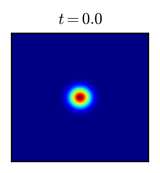
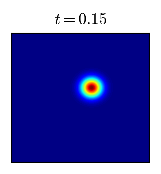
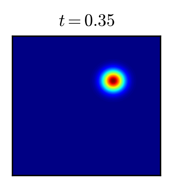
Figure 5: Numerical solution.

The dependence of the errors on the time step $\Delta t$ for a fixed $h$ is illustrated in Fig. 6. We observe that when $\Delta t$ is sufficiently small so that the assumption A5 of Theorem 19 is satisfied, the $L^{2}$ error behaves according to Remark 20 as $O(h^{k}+\Delta t^{q})$; so, the dominant part of the error for $q=1,2,3,4$ is the term $\Delta t^{q}$ because $k=5$; however, there are threshold values $\Delta t_{q}$ such that for $\Delta t\leq\Delta t_{q}$ the error is $0(h^{k})$, for instance, $\Delta t_{5}\simeq 2\cdot 10^{-2}$ and $\Delta t_{4}\simeq 10^{-2}$. The mass conservation errors behave approximately as $O(\Delta t^{q})$ for the non-conservative methods, which are significantly larger than those of the quasi-conservative methods when $1\leq q\leq 4$. In the latter methods and for $k\geq 3$ the mass conservation errors are approximately $O(h^{k})$; however, for $k=1$ and $2$ this rate is reached when $\Delta t$ is sufficiently small, say $\Delta t\simeq 10^{-2}$.

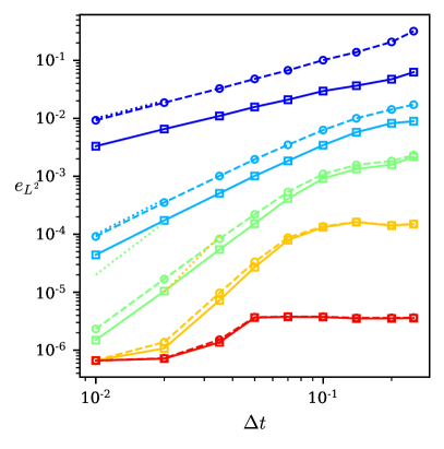
Figure 6: $L^{2}$ and mass errors with respect to $\Delta t$ for $k=5$ and $h=0.052$. Legend: ( ) $q=1$, ( ) $q=2$, ( ) $q=3$, ( ) $q=4$, ( ) $q=5$, ( ) present method, ( ) non-conservative scheme.

Fig. 7 illustrates the behavior of the errors with respect to the mesh size $h$ for a fixed time step $\Delta t$. In these examples the $L^{2}$ errors are almost coincident both for the conservative and the non-conservative methods. The $L^{2}$ error is now $O(h^{k+1}+\Delta t^{q})$; hence, for $h$ sufficiently small and $k\geq 4$ the dominant part of the error is $O(\Delta t^{q})$, this means that the error due to the time discretization becomes dominant. The mass conservation errors decrease when $h$ decreases, but with a somewhat oscillating behavior for $k=1$ and $2$ due perhaps to the fact that either $h$ or $\Delta t$ are not sufficiently small; however, for $k\geq 3$ and $h$ sufficiently small the error is $0(\Delta t^{q})$l as expected.

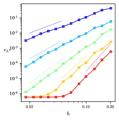
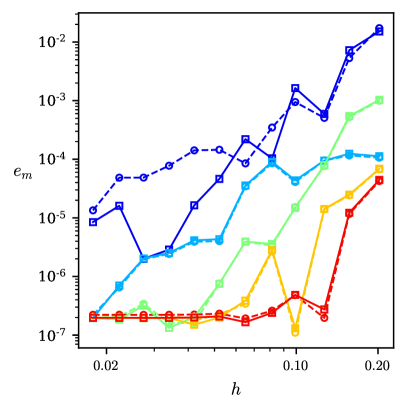
Figure 7: $L^{2}$ and mass errors with respect to $h$ for $q=4$ and $\Delta t=0.01$. Legend: ( ) $k=1$, ( ) $k=2$, ( ) $k=3$, ( ) $k=4$, ( ) $k=5$, ( ) present method, ( ) non-conservative scheme.

Finally, we have repeated the experiments of Rui and Tabata [39] in order to check the performance of our method versus the method proposed by these authors, which is based on the formulation (26) with $q=1$. In their experiments, the mesh is constructed by dividing each edge of the square domain into $N$ uniform segments, and $\Delta t=2/N$, for several values of $N$. The initial condition is taken as $c_{h}^{0}=L_{h}c^{0}$, with $L_{h}$ the Lagrange interpolation operator onto the finite element space $V_{h}$. Then, we measure the relative errors by the formulas

$$\widehat{e}_{L^{2}}=\displaystyle\dfrac{\max_{n}\sqrt{\int_{\Omega}\left(c_{h}^{n}-L_{h}c^{n}\right)^{2}d\Omega}}{\max_{n}\sqrt{\int_{\Omega}\left(L_{h}c^{n}\right)^{2}d\Omega}},\quad\widehat{e}_{m}=\displaystyle\dfrac{\left|\int_{\Omega}\left(c_{h}^{N_{T}}-L_{h}c^{N_{T}}\right)d\Omega\right|}{\left|\int_{\Omega}L_{h}c^{N_{T}}d\Omega\right|},$$

where $N_{T}=\lfloor T/\Delta t\rfloor$ denotes the last simulated time before $T$. Note that the authors in [39] employ a first-order-in-time method with linear elements. Since $\Delta t\sim h$ in these experiments, the $L^{2}$ error must converge as $O\left(\Delta t^{\min\{k,q\}}\right)$.

As seen in Fig. 8, the $L^{2}$ errors of our method are slightly larger than those of [39] for the case $k=q=1$. However, the former allows to consider higher-order discretizations that provide clearly better results. The $L^{2}$ error converges with $\Delta t$ as expected for $k=q\leq 4$; for $k=q=5$, the convergence is more irregular, although the errors are still smaller. The mass conservation errors are also smaller in our method.

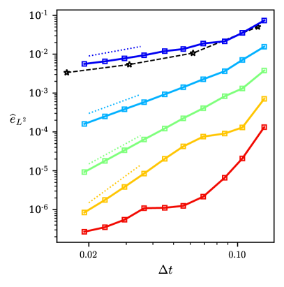
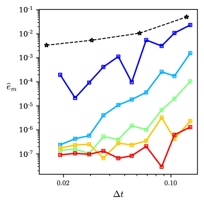
Figure 8: Relative $L^{2}$ and mass errors for the numerical experiments in [39]. Legend: ( ) $k=q=1$, ( ) $k=q=2$, ( ) $k=q=3$, ( ) $k=q=4$, ( ) $k=q=5$., ( ) Rui-Tabata method [39], ( ) present method.

Appendix

Finite element discretizations and $d$-curved simplices

The NCLG methods virtually move the elements of the fixed mesh backward in time thus generating elements with curved $d-$faces. Since we define finite element spaces associated with the meshes formed of such curve elements, then for the sake of completeness of the paper, we collect in this appendix, following the theory on curved elements of Bernardi [12], some results which are relevant for us.

The triple $(T,P(T),\Sigma_{T})$ is a finite element [16, Chapter 2.3], if: (i) $T$ is the closure of an open domain with Lipschitz piecewise smooth boundary, (ii) $P(T)$ is a finite dimensional space of real-valued functions defined over $T$, and (iii) $\Sigma_{T}$ is a set of continuous linear forms defined on $P(T)$ with support on $T$, and such that $\Sigma_{T}$ is $P(T)-$unisolvent, i.e., for any $\phi\in\Sigma_{T}$ there is one and only one $v\in P_{T}$ such that $\phi(v)=1$ and for any other $\phi^{\prime}\in\Sigma_{T}$, $\phi^{\prime}\neq\phi$, $\phi^{\prime}(v)=0$. Moreover we shall also consider the reference finite element $(\widehat{T},\widehat{P}(\widehat{T}),\widehat{\Sigma}_{\widehat{T}})$ where $\widehat{T}$ is the unit $d-$simplex, $\widehat{P}(\widehat{T})$ is the set of polynomials of degree $\leq k,\ k$ $\geq 0$ being an integer, and $\widehat{\Sigma}_{\widehat{T}}$ is a set of continuous linear forms with support on $\widehat{T}.$

Definition 21

([12], Definition 2.1) The $d-$simplex $T$ is said to be a curved $d-$simplex if there exists a $C^{1}$ mapping $F_{T}:\widehat{T}\rightarrow T$ such that

$$F_{T}=\overline{F}_{T}+\Theta_{T},$$ (80)

where

$$\begin{array}[]{c}\overline{F}_{T}:\widehat{T}\rightarrow\mathbb{R}^{d}\\ \widehat{x}\rightarrow\overline{B}_{T}\widehat{x}+\overline{b}_{T},\\ \overline{B}_{T}\in\mathcal{L}(\mathbb{R}^{d})\ \ \ \text{ and }\ \ \ \overline{b}_{T}\in\mathbb{R}^{d},\end{array}$$

is an invertible affine mapping and $\Theta_{T}:\widehat{T}\rightarrow\mathbb{R}^{d}$ is a $C^{1}$ mapping which satisfies

$$c_{T}=\sup_{\widehat{x}\in\widehat{T}}\parallel D\Theta_{T}(\widehat{x})\overline{B}_{T}^{-1}\parallel<1,$$ (81)

where $\left\|\cdot\right\|$ denotes the two-norm of the matrix.

Note that by the definition of $F_{T}$, a curved element $T$ can be considered as a perturbation to the element $\overline{T}=\overline{F}_{T}(\widehat{T})$. As usual, $h_{T}$, $h_{\overline{T}}$ and $\widehat{h}$ will denote $diam(T),\;diam(\overline{T})$ and $diam(\widehat{T})$ respectively. Moreover the definition allows the following result.

Lemma 22

([12], Lemma 2.1) The mapping $F_{T}$ is a $C^{1}$-diffeomorphism from $\widehat{T}$ onto $T$ that satisfies

$$\sup_{\widehat{x}\in\widehat{T}}\left\|DF_{T}(\widehat{x})\right\|\leq(1+c_{T})\left\|\overline{B}_{T}\right\|,$$ (82)

$$\sup_{x\in T}\left\|DF_{T}^{-1}(x)\right\|\leq(1-c_{T})^{-1}\left\|\overline{B}_{T}^{-1}\right\|,$$ (83)

$$\forall\widehat{x}\in\widehat{T},\ \ (1-c_{T})^{d}\left|\det\overline{B}_{T}\right|\leq\left\|\det DF_{T}(\widehat{x})\right\|\leq(1+c_{T})^{d}\left|\det\overline{B}_{T}\right|.$$ (84)

Furthermore. let $\widehat{\varrho}=$sup$\{$diam$(\widehat{S})$,$\ \widehat{S}$ a ball contained in$\ \widehat{T}\}$ and $\rho_{\overline{T}}$ the diameter of the maximum inscribed ball in $\overline{T}$, since [[16], Thm. 3.1.3]

$$\left\|\overline{B}_{T}\right\|\leq\frac{h_{\overline{T}}}{\widehat{\varrho}},\ \ \left\|\overline{B}_{T}^{-1}\right\|\leq\frac{\widehat{h}}{\rho_{\overline{T}}}\ \ \mathrm{and}\ \ \left|\det\overline{B}_{T}\right|=\frac{meas(\overline{T})}{meas(\widehat{T})},$$ (85)

it readily follows from (84) that

$$\sup_{\widehat{x}\in\widehat{T}}\left|\det DF_{T}(\widehat{x})\right|\leq\frac{1}{meas(\widehat{T})}\left(\frac{1+c_{T}}{1-c_{T}}\right)^{d}meas\left(T\right).$$ (86)

Also, there exist positive constants $c_{1}$ and $c_{2}$ depending on the $dx-$measure of the unit ball in $\mathbb{R}^{d}$ and the constant $C_{T}$ such that

$$c_{1}\rho_{\overline{T}}^{d}\leq meas(T)\leq c_{2}h_{\overline{T}}^{d}\text{.}$$

Definition 23

([12], Definition 2.2) A curved $d-$simplex is of class $C^{m}$, $m\geq 1$, if the mapping $F_{T}$ is of class $C^{m}$ on $\widehat{T}$.

For curved $d-$simplices of class $C^{m}$ there are constants

$$c_{l}(T)=\sup_{\widehat{x}\in\widehat{T}}\left\|D^{l}F_{T}(\widehat{x})\right\|\cdot\left\|\overline{B}_{T}\right\|^{-l},\ \ 2\leq l\leq m,$$ (87)

and constants $c_{-l}(T)$, which depend continuously on $c_{T},\ c_{2}(T),\ldots,c_{m}(T)$ such that

$$\sup_{x\in T}\left\|D^{l}F_{T}^{-1}(x)\right\|\leq c_{-l}\left\|\overline{B}_{T}\right\|^{2(l-1)}\left\|\overline{B}_{T}^{-1}\right\|^{l}.$$ (88)

We have the following lemma.

Lemma 24

([12], Lemma 2.3) Assume that $T$ is a curved element of class $m$ and let $k$ be an integer, $0\leq k\leq m$, and $p\in[1,\infty]$. A function $v$ is in $W^{k,p}(T)$ if and only if $\widehat{v}=v\circ F_{T}\in W^{k,p}(\widehat{T})$. Moreover, the following inequalities hold.

$$\left\{\begin{array}[]{l}\mid v\mid_{W^{k,p}(T)}\leq C\mid\det\overline{B}_{T}\mid^{1/p}\left(\sum_{r=0}^{k}\parallel\overline{B}_{T}^{-1}\parallel^{r}\mid\widehat{v}\mid_{W^{r,p}(\widehat{T})}\right),\\ \\ \mid\widehat{v}\mid_{W^{k,p}(\widehat{T})}\leq C\mid\det\overline{B}_{T}\mid^{-1/p}\parallel\overline{B}_{T}\parallel^{k}\left(\sum_{r=0}^{k}\mid v\mid_{W^{r,p}(T)}\right).\end{array}\right.$$ (89)

where the constants $C$ depend continuously on $c_{T}$ (see 81) and the constants $c_{l}.$

Definition 25

([12], Definition 2.4) The triplet $(T,P(T),\Sigma_{T})$ is said to be a curved finite element of order $m$ if:

(1)

$T$ is a curved $d-$simplex of class $C^{m+1}$, $P(T)$ is a finite dimensional space of functions from $T$ onto $\mathbb{R}^{d}$, and $\Sigma_{T}$ is the set of continuous linear forms defined on $\mathcal{D}(\mathbb{R}^{d})^{L}\oplus P(T)$ with support contained in $T$, $L$ being an integer $\geq 1$.

(2)

$P(T)=\{p(x),\ x\in T:p(x)=\widehat{p}\circ F_{T}^{-1}(x),\ \widehat{p}\in\widehat{P}_{m}(\widehat{T})^{L}\}$, where $\widehat{P}_{m}(\widehat{T})$ is the set of polynomials of degree $\leq m$ defined on $\widehat{T}$.

(3)

The set $\Sigma_{T}$ is $P(T)$-unisolvent; i.e., $\forall\mu\in\Sigma_{T}$ there is one and only one $p\in P_{T}$ such that $\mu(p)=1$ and $\forall\mu^{\prime}\in\Sigma_{T},\ \mu^{\prime}\neq\mu,\ \mu^{\prime}(p)=0$.

(4)

$P(T)\subset C^{m+1}(T)^{L}.$

Note that if all the boundaries of $T$ are straight $d-$faces, then all the statements of Definition 21 are valid with the only modification that $F_{T}:\ \widehat{T}\rightarrow T$ is now an invertible affine mapping.

Next, we summarize in the following definition some features of the family of partitions $(\mathcal{T}_{h})_{h}$ generated on $\overline{\Omega}$.

Definition 26

(1)

A family of partitions $(\mathcal{T}_{h})_{h}$ composed of curved $d-$simplices is said to be quasi-uniformly regular if there exist constants $\sigma,\ \nu$ and $c$ such that for each $h$ and $T$ in $\mathcal{T}_{h}$

$$\frac{h_{\overline{T}}}{\rho_{\overline{T}}}\leq\sigma,\ \ \frac{h}{h_{\overline{T}}}\leq\nu\text{ \ and \ }\sup_{h}\sup_{T\in D_{h}}c_{T}\leq c<1.$$

(2)

The family $(\mathcal{T}_{h})_{h}$ is said to be quasi-uniformly regular of order $m$, if it is quasi-uniformly regular and for each $h,$ any element $T$ in $\mathcal{T}_{h}$ is of class $C^{m+1}$ with (see (87))

$$\sup_{h}\sup_{T\in\mathcal{T}_{h}}c_{l}(T)<+\infty\ ,\ \ \ 2\leq l\leq m+1.$$

(3)

The partition $\mathcal{T}_{h}$ is said to be conformal if for any two elements $T_{l}$, $T_{k}$ of $\mathcal{T}_{h}$ such that $T_{l}\cap T_{k}=\Gamma^{lk}$, where $\Gamma^{lk}$ is a $(d-1)-$face, there is a face $\widehat{\Gamma}$ of $\widehat{T}$ such that $\Gamma^{lk}=F_{T_{l}}(\widehat{\Gamma})=F_{T_{k}}(\widehat{\Gamma})$ and $\left.F_{T_{l}}\right|_{\widehat{\Gamma}}=\left.F_{T_{k}}\right|_{\widehat{\Gamma}}$.

Given a partition $\mathcal{T}_{h}$ composed of curved $d-$simplices, in order to define an associated finite element space $V_{h}$ we shall take into account the set of linear forms

$$\Sigma_{h}=\bigcup_{T\in\mathcal{T}_{h}}\Sigma_{T},$$

and extract from $\Sigma_{h}$ a maximal system of linearly independent continuous forms $\{\mu_{i}\}_{i=1}^{M}$. Then, for $1\leq$ $i\leq M$, let

$$\Delta_{i}=\bigcup_{T\in\mathcal{T}_{h}}\left\{T:\sup p(\mu_{i})\subset T\right\}.$$

If the family $(\mathcal{T}_{h})_{h}$ is regular, we have that for any two elements $T$ and $T^{\prime}$ contained in $\Delta_{i}$ there is a constant $C$ such that $h_{\overline{T}}\leq Ch_{\overline{T}^{\prime}}$. By virtue of Definition 25, for each $i,\ 1\leq i\leq M$, there exists a unique function $\chi_{i}$ such that $\forall T\in\mathcal{T}_{h}$,$\ \chi_{i}\mid_{T}\in P(T)$ and $\mu_{j}(\chi_{i})=\delta_{ji}$. The set $\{\chi_{i}\}_{i=1}^{M}$ is the set of global basis functions for the finite element space $V_{h}$, i.e.,

$$V_{h}=Span\{\chi_{i},\ 1\leq i\leq M\}.$$

Definition 27

([12], Definition 3.3) The curved finite elements of order $m$ $(T,P(T),\Sigma_{T}),\ T\in\mathcal{T}_{h}$, associated with the family of partitions $(\mathcal{T}_{h})_{h}$ are said to be compatible if:

(1)

The dimensions of $P(T)$ are bounded independently of $h$.

(2)

Let $\Delta_{i}$ denote the support of the basis function $\chi_{i}$ in the partition $\mathcal{T}_{h}$ , i.e., $\Delta_{i}=\bigcup_{T\in\mathcal{T}_{h}}\{T:supp(\chi_{i})\cap T\neq\emptyset\}$. Then, for all $i,1\leq i\leq M$ , either $\Delta_{i}$ is contained in an element $T$ or $\mu_{i}$ can be extended to a continuous linear form on $C(\Delta_{i}).$

(3)

For all $i,\ 1\leq i\leq M$, there exists a constant $K$ independent of $h$ such that

$$\forall\rho\in P(T),\ \mid\mu_{i}(\rho)\mid\leq Kh_{T}^{r_{i}-d/p_{i}+s_{i}}\parallel\rho\parallel_{W^{r_{i},p_{i}}(T)},$$

where $r_{i}$ is an integer $\geq 0$, $p_{i}\in[1,+\infty],$ and $s_{i}$ is a real number. Moreover, $\forall k,\ 0\leq k\leq m+1\$and $\forall q\in[1,+\infty]$

$$\parallel\chi_{i}\parallel_{k,q,T}\leq Kh_{T}^{-k+d/q-s_{i}},$$

for any element $T$ contained in $\Delta_{i}.$

Let $W(\Omega)$ be a Banach space of functions defined on $\Omega\rightarrow\mathbb{R}^{L}\$(actually, $W(\Omega)\$ is a Banach space associated with a sheaf-$W$ of functions defined on the domains in $\mathbb{R}^{d}$, see [12] for further information).

Definition 28

([12], Definition 5.1) A finite element $(T,P(T),\Sigma_{T})$ is said to be $W$-conformable if:

(1)

$P(T)\subset W(T)$.

(2)

For each face $\Gamma^{j}\ (1\leq j\leq d+1)$ of $T$, there exists a subset $\Sigma_{T,\Gamma^{j}}$ of $\Sigma_{T}$ such that:

(i)

For any $u\in\{\mathcal{D}(\mathbf{\mathbb{R}}^{d})^{L}\oplus P(T)\}\cap W(T)$ and for any $\mu$ in $\Sigma_{T,\Gamma^{j}}$, $\mu(u)$ depends only on $L_{T}(u)\mid_{\Gamma^{j}}$, where $L_{T}$ is a trace operator defined on $W(T)$;

(ii)

For any $p\in P(T),\ \{\forall\mu\in\Sigma_{T,\Gamma^{j}},\ \mu(p)=0\}\Rightarrow\{L_{T}(p)\mid_{\Gamma^{j}}=0\}$.

For straight $d-$simplices this definition means that the triplet $(\Gamma^{l},\ L_{T}(P_{T})\mid_{\Gamma^{l}},\ \Sigma_{T,\Gamma^{l}})$ is a finite element.

We also need the definition of $W$-conforming finite elements.

Definition 29

([12], Definition 5.2) The $W$-conformable finite elements $(T,P(T),\Sigma_{T})$, $T\in\mathcal{T}_{h}$, associated with the family of partitions $(\mathcal{T}_{h})_{h}$ are said to be $W$-conforming, if for each $h$ and for any triangles $T$ and $T^{\prime},$ such that $T\cap T^{\prime}=\Gamma$, the spaces $L_{T}(P(T))\mid_{\Gamma}$ and $T_{\varepsilon}L_{T^{\prime}}(P(T^{\prime}))\mid_{\Gamma}$ are the same, and the sets $\Sigma_{T,\Gamma}$ and $\Sigma_{T^{\prime},\Gamma}$ span the same subspace of $D^{\prime}(\mathbb{R}^{2})^{L}$. Here, $T_{\varepsilon}$ is the involution operator in $\mathbf{\mathbb{R}}^{s}$ : $(\xi)=(\xi_{i})_{1\leq i\leq s}\rightarrow\mathbf{(}\varepsilon_{i}\xi_{i})_{1\leq i\leq s}$, with the k-tuple $\varepsilon=(\varepsilon_{i})_{1\leq i\leq k}\in[-1,1]^{s}$.

We are now in a position to introduce  the finite element spaces associated with the family of partitions $(\mathcal{T}_{h})_{h}$.

$$V_{h}:=\{v_{h}\in C(\overline{\Omega}):\ v_{h}\mid_{T}\in P(T)\ \forall T\in\mathcal{T}_{h}\},$$ (90)

with

$$P(T):=\{p(x):p(x)=\widehat{p}\circ F_{T}^{-1}(x),\ \widehat{p}\in\widehat{P}_{m}(\widehat{T})\}\text{, }$$ (91)

and $F_{T}:\widehat{T}\rightarrow T$ is such that if $T$ is a curved element, then $F_{T}$ is a mapping of class $C^{m+1}$ defined by (80). We must note that since the finite elements $(T,P(T),\Sigma_{T})$ are $H^{1}$-conforming, then $V_{h}\subset H^{1}(\Omega)$ as shown in Proposition 5.1 of [12]. To state the approximation properties of finite element spaces with $W$-conforming curved elements of order $m$ we shall use Lemma 24 and follow the methodology of Chapters 3 and 4 of [16]. Thus, let $T$ be a curved element of class $m$ and let $v$ be a function defined on $T$ such that $v=\widehat{v}\circ F_{T}^{-1}$, where the function $\widehat{v}$ is defined on the reference element $\widehat{T}$ and $F_{T}$ is the mapping of class $C^{m+1}$ defined by (80) and (81), then one can estimate $v-\Pi_{T}v$, $\Pi_{T}$ being an interpolation operator. We have the following theorem.

Theorem 30

Let there be given the following items:

(1)

a curved finite element of order $m$ $(T,P(T),\Sigma_{T})$ and the reference finite element $(\widehat{T},\ \widehat{P}_{k}(\widehat{T}),\ \widehat{\Sigma}_{\widehat{T}})$;

(2)

an integer $l\geq 0$ and two numbers $p,\ q\in[1,\infty]$ such that the following inclusions hold:

$$W^{m+1,p}(\widehat{T})\hookrightarrow C(\widehat{T})\text{ and }W^{m+1,p}(\widehat{T})\hookrightarrow W^{l,q}(\widehat{T});\$$

(3)

the interpolation operator $\widehat{\Pi}_{\widehat{T}}\in\mathcal{L}(W^{m+1,p},W^{l,q})$ satisfying $\forall\widehat{p}\in\widehat{P}_{k}(\widehat{T})$, $\widehat{\Pi}_{\widehat{T}}\widehat{p}=\widehat{p}$;

(4)

the interpolation operator $\Pi_{T}:C^{0}(T)\rightarrow\mathbf{\mathbb{R}}^{L},$ such that for $v\in dom\Pi_{T}$ and $\widehat{v}\in dom\widehat{\Pi}_{\widehat{T}}$, with $v=\widehat{v}\circ(F_{T})^{-1}$, $(\Pi_{T}v)^{\widehat{}}=\widehat{\Pi}_{\widehat{T}}\widehat{v}.$

Then, there exists a constant $C(\widehat{\Pi}_{\widehat{T}},\widehat{T})$ such that $\forall v\in W^{m+1,p}(T)$

$$\mid v-\Pi_{T}v\mid_{W^{l,q}(T)}\leq Ch_{\overline{T}}^{d(\frac{1}{q}-\frac{1}{p})+m+1-l}\left(\sum_{r=0}^{m+1}\mid v\mid_{W^{r,p}(T)}\right).$$ (92)

From Corollary 4.1 of [12], see also Theorem 4.28 of [21], we can obtain an estimate of the interpolation error for the finite element spaces $V_{h}$ associated with an exact conforming quasi-uniformly regular family of partitions $(\mathcal{T}_{h})_{h}$.

Theorem 31

Let $V_{h}$ be a family of finite element spaces associated with a complete regular family of partitions $(\mathcal{T}_{h})_{h}$. $V_{h}$ is made up of compatible $H^{1}$-conforming curved finite elements of order $m$. Let $\Pi_{h}:C(\mathbb{R}^{d})\rightarrow V_{h}$ be an interpolation operator such that $\Pi_{h}v\mid_{T}=\Pi_{T}v$ and for all $\mu_{i}\in\Sigma_{T}\$ $\mu_{i}(\Pi_{h}v)=v(a_{i})$, where $a_{i}$ are the mesh points on $T$. Then, for $\ l$ and $k$ integers with $l\geq 0$, $0\leq k\leq m$, $p,\ q\in[1,\infty]$,$\ v\in W^{m+1,p}(\Omega)$ and $v-\Pi_{h}v\in W^{l,q}(\Omega)$ with $W^{k+1,p}(\Omega)\hookrightarrow W^{l,q}(\Omega)$, it holds

$$\left(\sum_{T\in\mathcal{T}_{h}}\left|v-\Pi_{h}v\right|_{W^{l,q}(T)}^{p}\right)^{1/p}\leq Ch^{d(\frac{1}{q}-\frac{1}{p})+k+1-l}\left\|v\right\|_{W^{k+1,p}(\Omega),}$$ (93)

where $0<h=\max_{T}\{h_{\overline{T}}\}\leq 1$.

References

[1] A. Allievi and R. Bermejo, A generalized particle search-locate
algorithm for arbitrary grids. J. Comp. Phys., 132: 157-166, 1997.
[2] G. Akrivis, Stability of implicit-explicit backward difference
formulas for nonlinear parabolic equations. SIAM J. Numer. Anal., 53:
464-484, 2015.
[3] G. Akrivis, M. Chen, F. Yu and Z. Zhou, The energy technique
for the sixth-step BDF method. SIAM J. Numer. Anal., 59: 2449-2472, 2021.
[4] A. Alphonse, C. M. Elliot and B. Stinner, An abstract
framework for parabolic PDEs on evolving spaces. Port. Math., 72: 1-46, 2015.
[5] M. Bause and P. Knabner, Uniform error analysis for
Lagrange-Galerkin approximations of convection-dominated problems. SIAM J.
Numer. Anal., 39: 1954-1984, 2002.
[6] R. Bermejo and J. Carpio, A semi-Lagrangian-Galerkin projection
scheme for convection equations. IMA Journal of Numerical Analysis, 30:
799-831, 2010.
[7] R. Bermejo, P. Galán del Sastre and L. Saavedra, A second
order in time modified Lagrange-Galerkin finite element method for the
incompressible Navier-Stokes equations. SIAM J. Numer. Anal., 50: 3084-3109,
2012.
[8] R. Bermejo and L. Saavedra, Modified Lagrange-Galerkin methods
of first and second order in time for convection-diffusion problem. Numer.
Math., 120: 601-638, 2012.
[9] R. Bermejo and L. Saavedra, Modified Lagrange-Galerkin methods
to integrate time dependent incompressible Navier-Stokes equations. SIAM J.
Sci. Comput., 37: B779-B803, 2015.
[10] R. Bermejo and L. Saavedra, A second order in time local
projection stabilized Lagrange-Galerkin method for Navier-Stokes equations
at high Reynolds numbers. Computers and Mathematics with Applications, 72:
820-845, 2016.
[11] A. Bermúdez, M.R. Nogueiras and C. Vázquez,
Numerical analysis of convection-diffusion-reaction problems with higher
order characteristics/finite elements. Part II: Fully discretized scheme and
quadrature formulas. SIAM J. Numer. Anal., 44: 1854-1876, 2006.
[12] C. Bernardi, Optimal finite-element interpolation on curved
domains. SIAM J. Numer. Anal., 26: 1212-1240, 1989.
[13] K. Boukir, Y. Maday, B. Métivet and E. Razanfindrakoto,
A high-order characteristics/finite element method for the incompressible
Navier-Stokes equations. International J. Numer. Methods Fluids, 25:
1421-1454, 1997.
[14] A. N. Brooks and T.J.R. Hughes, Streamline
upwind/Petrov-Galerkin formulations for convection dominated flows with
particular emphasis on the incompressible Navier-Stokes equations. Comput.
Meth. Appl. Mech. Engrg. 32: 199-259, 1982.
[15] K. Chrysafinos and N.J. Walkington, Lagrangian and moving mesh
methods for the convection diffusion equation. ESAIM: M2AN, 22: 25-65, 2008.
[16] P. G. Ciarlet, The Finite Element Method for Elliptic
Problems, North-Holland, Amsterdam, 1978.
[17] A. J. Chorin and J. E. Marsden, A Mathematical
Introduction to Fluid Mechanics, Springer-Verlag Berlin, 1984.
[18] M. Colera, J. Carpio and R. Bermejo, A nearly-conservative
high-order Lagrange-Galerkin method for the resolution of scalar
convection-dominated equations in non-divergence-free velocity fields.
Comput. Meth. Appl. Mech. Engrg., 372, 113366, 2020.
[19] T. Dupont, G. Fairweather and J. P. Johnson, Three-level
Galerkin methods for parabolic equations. SIAM J. Numer. Anal., 11: 392-410,
1974.
[20] J. Douglas and T. F. Russell, Numerical methods for
convection-dominated diffusion problems based on combining the method of
characteristics with finite element or finite difference procedures. SIAM J.
Numer. Anal., 19: 871-885, 1982.
[21] C. M. Elliot and T. Ranner, A unified theory for continuous in
time evolving finite element space approximations to partial differential
equations in evolving domains. IMA Journal of Numerical Analysis, 41:
1696-1845, 2021.
[22] C. M. Elliot and T. Ranner, Finite element analysis for a
coupled bulk-surface partial differential equation. IMA Journal of Numerical
Analysis, 33: 377-402, 2013.
[23] A. Ern and J-L. Guermond, Theory and Practice of Finite
Elements, Springer Applied Mathematical Science 159, Springer-Verlag,
New-York, 2004.
[24] L. C. Evans, Partial Differential Equations,
American Mathematical Society, 1998.
[25] R. Ewing and T. F. Russell, Multistep Galerkin methods along
characteristics for convection-diffusion problems, in Advances in
Computer Methods for Partial Differential Equations IV, R. Vchtneveski and
R.S Stepleman eds., IMACS, New Brunswick, NJ., 28-36, 1981.
[26] K. Futai, N. Kolbe, H. Notsu and T. Suzuki, A mass preserving
two-step Lagrange-Galerkin scheme for convection-diffusion problems. J. Sci.
Comput., 92: 37, 2022.
[27] P. Hansbo, The characteristic streamline diffusion method
for convection-difusion problems. Comput. Meth. Appl. Mech. Engrg., 96:
239-253, 1992.
[28] E. Hairer, S. P. Norsett and G. Wanner, Solving
Odinary Differential Equations I, Springer-Verlag, Berlin, 1991.
[29] P. Hartman, Ordinary Differential Equations, Wiley,
New York, 1973.
[30] T.J.R. Hughes, L.P. Franca and G. M. Hulburt, A new finite
element formulation for computational fluid dynamics: VIII the
Galerkin/least squares method for advection-diffusive equations. Comput.
Meth. Appl. Mech. Engrg. 73: 173-189, 1989.
[31] J. G. Heywood and R. Rannacher, Finite element approximations
of the nonstationary Navier-Stokes problem IV. SIAM J. Numer. Anal., 27:
353-384 1990.
[32] C Johnson, A new approach to algorithms
for convection problems which are based on exact transport+projection.
Comput. Meth. Appl. Mech. Engrg., 100: 45-62, 1992.
[33] I. Malcevic and O. Ghattas, Dynamic-mesh finite element method
for Lagrangian computational fluid dynamics. Finite Elements Analysis and
Design. 38: 965-982, 2002.
[34] V. G. Maz’ja, Sobolev Spaces, Springer-Verlag,
Berlin, 1985.
[35] O. Nevanlinna and F. Odeh, Multiplier techniques for linear
multistep methods. Numer. Funct. Anal. Optim., 3: 377-423, 1981.
[36] O. Pironneau, On the transport-diffusion algorithm and its
applications to the Navier-Stokes equations. Numer. Math., 38: 309-332, 1982.
[37] A. Quarteroni and A. Valli, Numerical
Approximation of Partial Differential Equations, Springer Ser. Comput.
Math. 23, Springer-Verlag, Berlin, 1994
[38] H. Rui and M. Tabata, A second order characteristic finite
element scheme for convection-diffusion problems. Numer. Math., 92: 161-177,
2002.
[39] H. Rui and M. Tabata, A mass-conservative characteristic
finite element scheme for convection-diffusion problems. J. Sci. Comput.,
43: 416-432, 2010.
[40] E. Süli, Convergence and nonlinear stability of the
Lagrange-Galerkin method for the Navier-Stokes equations. Numer. Math., 53:
459-483, 1988.
[41] V. Thomée, Galerkin Finite Element Methods for
Parabolic Problems, Springer-Verlag, Berlin, 1997.