Dataset Difficulty and the Role of Inductive Bias

Abstract

Motivated by the goals of dataset pruning and defect identification, a growing body of methods have been developed to score individual examples within a dataset. These methods, which we call “example difficulty scores”, are typically used to rank or categorize examples, but the consistency of rankings between different training runs, scoring methods, and model architectures is generally unknown. To determine how example rankings vary due to these random and controlled effects, we systematically compare different formulations of scores over a range of runs and model architectures. We find that scores largely share the following traits: they are noisy over individual runs of a model, strongly correlated with a single notion of difficulty, and reveal examples that range from being highly sensitive to insensitive to the inductive biases of certain model architectures. Drawing from statistical genetics, we develop a simple method for fingerprinting model architectures using a few sensitive examples. These findings guide practitioners in maximizing the consistency of their scores (e.g. by choosing appropriate scoring methods, number of runs, and subsets of examples), and establishes comprehensive baselines for evaluating scores in the future.

1 Introduction

As artificial neural networks and the datasets used to train them have rapidly increased in size and complexity, it has become increasingly important to identify which examples affect learning and how. Indeed, in recent years a growing number of proposals have appeared for scoring and ranking individual examples in the training set in order to identify which examples may suffer from catastrophic forgetting (Toneva et al.,, 2019), are affected by network pruning (Jin et al.,, 2022), contribute to improved generalization (Paul et al.,, 2021; Nohyun et al.,, 2023; Sorscher et al.,, 2022; Swayamdipta et al.,, 2020), improve downstream model robustness (Northcutt et al.,, 2021; Jiang et al.,, 2020), or help in mitigating biases in the model (Hooker et al.,, 2019, 2020). A common theme among these scores is that the most “difficult” (e.g. highest error) examples often significantly affect learning, while a substantial fraction of “easy” (lowest error) examples can be discarded without adversely affecting model properties such as test accuracy. Beyond direct applications such as data pruning, where a fraction of a large dataset can be used to train models to equivalent performance (Toneva et al.,, 2019; Hooker et al.,, 2020; Paul et al.,, 2021; Nohyun et al.,, 2023; Sorscher et al.,, 2022), these methods can be used to identify outliers (Carlini et al.,, 2019; Feldman and Zhang,, 2020; Siddiqui et al.,, 2022; Paul et al.,, 2021), find underrepresented classes of examples (Hooker et al.,, 2020), correct for biases and spurious correlations (Yang et al.,, 2023), remove mislabelled or redundant examples (Pleiss et al.,, 2020; Birodkar et al.,, 2019; Pruthi et al.,, 2020; Jiang et al.,, 2020; Swayamdipta et al.,, 2020), and prioritize important examples in training through curriculum-based learning (Paul et al.,, 2021; Jiang et al., 2019a, ).

There exists a plethora of scores targeting various applications, but regardless of their uses, one needs a good grasp of their properties and robustness in order to use scores appropriately. We thus take the application of each score out of the question, and instead evaluate how scores vary between runs, how they relate to one another, and how transferable they are between different model architectures. Since each score implicitly or explicitly ranks training examples by their “difficulty”, we refer to these scores as example difficulty scores. That said, the difficulty of an example cannot be defined independently, since scores vary depending on the rest of the training data, the inductive biases of the model, and the training algorithm. Many scores also require additional information from the data or model such as gradient information (Paul et al.,, 2021), gradient variance among the training data (Agarwal et al.,, 2020), the training trajectory (Siddiqui et al.,, 2022), or the error signal (Toneva et al.,, 2019; Swayamdipta et al.,, 2020).

From a research standpoint, our study sets a foundation for comparing example difficulty scores by establishing a proper evaluation protocol and baselines against which new scores can be compared. In particular, we ask how much do example rankings vary due to random effects (e.g. model initialization), and do different scores measure independent notions of difficulty (i.e. how correlated are their example rankings)? From a practical standpoint, our answers to these questions may help practitioners determine which scores to choose based on the downstream use and their desired robustness/invariance (e.g., to architectures), how many runs are needed to rank examples reliably, and whether a compute-costly score can be interchanged for a cheaper one. A practitioner may also want to know if rankings are consistently affected by changes to the model (e.g., the size of a neural network) or hyperparameters in the learning algorithm (e.g., learning rate in stochastic gradient methods) Paul et al., (2021); Jiang et al., (2020)—properties which we call the inductive biases of the model. To address this question, we consider how example difficulty changes in response to different inductive biases, and whether this difference is detectable above the random variation due to different runs. We summarize our findings below.

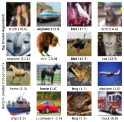
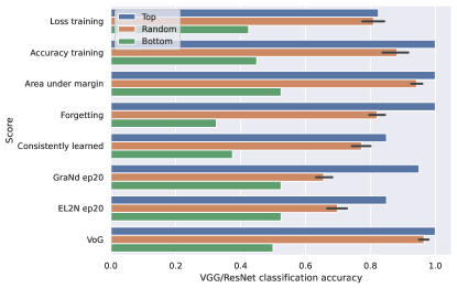
Figure 1: Left: Top 8 CIFAR-10 examples most/least sensitive to inductive biases (model width, depth, and architecture), ranked by statistical significance of changes to difficulty score for pairwise model comparisons (see Section 4.3 for more details). Numbers indicate mean $-\log P$ value of each example. Right: Distinguishing between VGG and ResNet using the top 8 examples (Left) as features for logistic regression.

Key contributions:

1. There is substantial variance in difficulty between different runs (due to random initialization, etc.), and this variation is generally higher for harder examples (Figure 2). As a result, ranking or thresholding examples is unreliable when scores are averaged over a small number of runs (Figure 3).

2. All difficulty scores are generally well correlated with themselves and other scores (Figure 4). Averaging over multiple runs almost always improves this correlation (gradient-based scores are an exception).

3. A single principal component captures most of the variation in difficulty among scores computed on training examples (Figure 5). The remaining variation is independent between scores and cannot be reduced by linear combination to make data ranking/thresholding more consistent.

4. Different types of models with distinct inductive biases cause statistically significant changes in difficulty for many examples. Scores from as few as 8 examples can be used as a fingerprint to reliably distinguish between inductive biases (Figure 1).

These results highlight several underappreciated aspects of using difficulty scores in practice. First, ranking or classifying individual examples (e.g. to identify mislabelled examples) is error-prone, since the per-run variance of scores is high and differs from example to example. The cost of training large models may additionally limit the number of runs (e.g. 5-10) on which scores are averaged, worsening this issue.

Second, all scores are fairly predictive of one another in spite of their methodological differences. A key motivation for many scores is to be a proxy for other, more computationally-intensive scores Paul et al., (2021); Jiang et al., (2020); Pleiss et al., (2020); Agarwal et al., (2020); Baldock et al., (2021); Sorscher et al., (2022). Our work shows that the correlation between proxy scores needs to be quite high to beat the baseline similarity among unrelated scores.

Finally, the role of the model has typically been ignored or averaged out in practice. Drawing inspiration from statistical genetics, we show that models affect example difficulty in predictable ways. We find that a handful of examples with the most significant changes can reliably distinguish between inductive biases, giving practitioners a new tool for fingerprinting different models. Conversely, practitioners should be wary of comparing scores from different models, since only a minority of examples have model-independent scores.

2 Methodology

We seek to tease apart the influence of various factors on example difficulty: namely, the role of uncontrolled/random effects (e.g. model initialization), the scoring method, and controlled effects (e.g. model architecture). These factors naturally divide our experiments into measuring the variance, covariance, and bias of scores.

2.1 Variance

Scores are often averaged over many runs to increase their consistency. However, with large models the number of runs is often limited by computational resources. In this situation a practitioner might ask: how many runs correspond to a given level of error in estimated score, and given a choice of scores, which ones are least affected by per-run variance?

While prior work shows that some scores are consistent over different runs (Baldock et al.,, 2021), such as by calculating between-run correlations (Toneva et al.,, 2019), a baseline is needed to understand what degree of consistency is to be generally expected. Furthermore, the degree to which some examples are less consistent than others is unknown. To address these issues, we plot the distribution of per-run score variance for all examples (Section 4.1, Figure 2) to understand how score error changes at different levels of difficulty, and the effects of this error in the two common applications of splitting and ranking data (e.g. for data pruning, outlier detection, and training prioritization).

For extremely large models where multiple runs are impractical (e.g. Dosovitskiy et al., (2021)), practitioners may also want to know whether individual runs can reliably estimate the average score of an example, or predict other types of scores or the outcome of other runs. To address this, we compute pairwise correlations between scores on a mean-to-mean, mean-to-run, and run-to-run basis (Section 4.2, Figure 4) to cover all combinations of predictions between scores from single/multiple runs.

2.2 Covariance

The large variety of difficulty scores with distinct formulations makes it difficult to understand which scores are appropriate for a given task. Simple scores are also preferred over compute-expensive scores (such as those averaged over an ensemble of models) if they are more or less equivalent. Practitioners may therefore ask: how do different scores relate to each other, and do they measure the same notion(s) of difficulty?

Previous works address these questions to a limited extent, such as the error norm (EL2N) being strongly correlated with the gradient norm (GraNd) and forgetting score (Paul et al.,, 2021), or prediction depth correlating well with example learning times and adversarial margins (Baldock et al.,, 2021). Again however, a baseline is needed to understand what score substitutions are possible and the general level of similarity expected between scores. The pairwise correlations between scores in Figure 4 establish this baseline, enabling existing and newly proposed scores to be compared by their similarity and ability to predict other scores.

To better understand what scores are actually measuring, practitioners may also want to know if there are multiple ways that examples can vary in difficulty, such as by counting the orthogonal directions covered by different scores. Prior works have tended to propose two dimensions of difficulty (Hooker et al.,, 2019; Carlini et al.,, 2019; Baldock et al.,, 2021; Swayamdipta et al.,, 2020), often related to train versus test set performance, but it is unknown if the dimensions proposed by these works are equivalent. Although we only consider training examples in this work, we make a first step towards quantifying the dimensionality of difficulty scores by measuring the principal components of variation spanned by a variety of scores, and the degree to which different scores share principal components (Section 4.2, Figure 5).

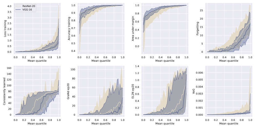
Figure 2: Variance of selected difficulty scores for CIFAR-10 examples. Rows 1-2: Score distribution for individual examples (y-axis) and individual runs, ordered by the rank of their mean score (x-axis). To make the plots more legible, examples are binned into groups of 1000. Shaded region indicates 90% confidence interval. From top to bottom and left to right: mean loss over training, mean accuracy over training, area under margin (correct class probability minus top other class) over training, number of forgetting events, epoch when example is learned without further forgetting, gradient norm at epoch 20, $L^{2}$ norm of output probability error at epoch 20, mean per-pixel variance of gradients at input over training.

2.3 Bias

The difficulty of an example depends on both properties of the example and the function class used to model it, such as the architecture of the model. For example, it is clear that a simple logistic regression and a large convolutional network would produce very different difficulty scores, and that their relative performance could shift drastically on images versus linearly separable data. However, if two models have comparable average performance, the degree to which difficulty scores evaluated on each model differ is not so obvious.

Prior work highlights how some scores tend to not vary among different model architectures (Carlini et al.,, 2019; Paul et al.,, 2021; Baldock et al.,, 2021), but a comprehensive evaluation of the robustness of scores to different model architectures is lacking. We also note that model-dependent scores may be desirable for some applications, such as identifying the inductive biases of a model. To better understand the full range of model-dependent effects, we ask: which scores and examples are more sensitive to a model’s inductive bias, and conversely, which ones are more model-agnostic? We address these questions by conducting a large-scale statistical analysis of the change in score between different model architectures at the level of individual examples (Section 4.3, Figure 6). This allows us to find particular examples which are extremely sensitive/insensitive to inductive biases, which can be used as a “fingerprint” to classify model architectures with only a few scores (Figure 1).

3 Difficulty Scores and Related Work

We provide a brief overview of difficulty scores, focusing on their conceptual relations. Since the variance of a score depends strongly on sample size, we categorize scores by their sampling method:

• Scores computed at a single point in training. This category includes typical performance metrics computed at the end of training, such as accuracy. Since large models effectively have zero training loss, more sophisticated scores are needed to differentiate examples, including prediction depth (Baldock et al.,, 2021), adversarial robustness (Carlini et al.,, 2019), and normalized margin from decision boundary (Jiang et al., 2019b, ). Scores can also be computed during training for applications such as data pruning, including the $L^{2}$ norm of the gradient with respect to model parameters, or the norm of the output error (Paul et al.,, 2021). Although scores in this category can also be averaged over training, they are typically evaluated at specific times for a specific purpose such as model evaluation.

• Scores computed throughout training. These are scores requiring multiple model evaluations throughout training. Sampling methods include evaluating all examples at fixed intervals (e.g. per epoch), or evaluating each minibatch of examples when they are used in training (Toneva et al.,, 2019). Simple pointwise evaluations which can be averaged over all samples include loss (Jiang et al.,, 2020), accuracy (Jiang et al.,, 2020), entropy (Jiang et al.,, 2020), model confidence (Jiang et al.,, 2020; Carlini et al.,, 2019; Swayamdipta et al.,, 2020), and the classification probability margin (Toneva et al.,, 2019; Jiang et al.,, 2020; Pleiss et al.,, 2020). Derived quantities include the variance of the above quantities over training (Swayamdipta et al.,, 2020), the number of forgetting events (Toneva et al.,, 2019), the time when an example is learned (Toneva et al.,, 2019) or remains consistently learned (Baldock et al.,, 2021; Siddiqui et al.,, 2022), and the use of entire loss trajectories as features for a downstream classifier (Siddiqui et al.,, 2022). Gradient-based methods include the variance of gradients (VoG) at the input (Hooker et al.,, 2020).

• Scores computed from an ensemble of models. We omit scores from the previous categories since they can also be trivially averaged over an ensemble of models. Methods that average over different train/test splits include ensemble accuracy (Meding et al.,, 2021), train/test split consistency (Jiang et al.,, 2020), influence and memorization (Feldman and Zhang,, 2020), and retraining on held-out data (Carlini et al.,, 2019). Other scores include agreement in mutual information over an ensemble (Carlini et al.,, 2019; Kalimeris et al.,, 2019), robustness to $\epsilon$-differential privacy (Carlini et al.,, 2019), and true-positive agreement (Hacohen et al.,, 2020). Finally, scores that measure sensitivity to model perturbations include compression- and pruning-identified exemplars (Hooker et al.,, 2019).

• Training-free scores. These scores are computed either with a closed-form expression or an arbitrarily chosen model, and are thus independent of the training process. Examples include the complexity gap (Nohyun et al.,, 2023) and supervised/self-supervised prototypes (Sorscher et al.,, 2022).

As the list above is too broad to exhaustively analyze, we restrict the scope of our work as follows. Firstly, we only look at models during training, excluding scores that require other model or data perturbations such as model pruning, model compression, or adversarial attacks.

Whether an example is seen by the model during training has obvious effects on its computed difficulty (Baldock et al.,, 2021; Feldman and Zhang,, 2020; Hacohen et al.,, 2020; Carlini et al.,, 2019). More subtly, the exact contents of the training dataset will also influence an example’s difficulty (Feldman and Zhang,, 2020; Carlini et al.,, 2019). Our analysis uses default train/test splits and only scores training examples. For ease of comparison, we include some precomputed scores from other works such as Carlini et al., (2019); Feldman and Zhang, (2020).

Based on these restrictions, we select a representative subset of difficulty scores for the main text:

• Loss and Accuracy: average loss and zero-one accuracy over training (Jiang et al.,, 2020).

• Area under margin: the mean difference (over training) between the model’s true class confidence (probability after softmax) and the highest confidence on any other class (Pleiss et al.,, 2020).

• Forgetting and Consistently learned: the number of times an example is forgotten (changes from correct to incorrectly classified) over successive minibatches (Toneva et al.,, 2019), and the first time an example is learned without further forgetting (also called iteration learned) (Baldock et al.,, 2021; Siddiqui et al.,, 2022).

• GraNd ep20 and EL2N ep20: the gradient norm and approximation of the norm as the $L^{2}$ norm of the error in output probability (Paul et al.,, 2021). As these scores are used for early data pruning, we follow the original authors and compute them at epoch 20.

• VoG: (variance of gradients) measuring the mean variance of gradients with respect to individual input pixels (Agarwal et al.,, 2020).

• Ensemble agreement and Holdout retraining: also called “agr” and “ret” in Carlini et al., (2019), these are precomputed scores for the Jensen-Shannon divergence between outputs in an ensemble, and the drop in KL-divergence when a trained model is fine-tuned on a hold-out dataset where the example in question is removed.

4 Experiments and Results

All figures in the main text are for scores computed with ResNet-20 (He et al.,, 2016) models trained on CIFAR-10 (Krizhevsky,, 2009). Difficulty scores are computed over 40 replicates for each model/dataset using standard SGD training for 160 epochs.

For experiments measuring inductive bias, we additionally run 20 replicates of variations on ResNet (He et al.,, 2016) and VGG (Simonyan and Zisserman,, 2015) models with increased/reduced width/depth which are as follows: ResNet wide (ResNet-20-64, or $4\times$ width), ResNet deep (ResNet-34), VGG narrow (VGG-16-16, or $1/4\times$ width), and VGG shallow (VGG-11).

4.1 Variance of Scores

We first examine the distribution of per-example scores over individual runs. Figure 2 shows the 90% confidence interval for scores binned by the quantile of their mean score over all runs. A few general trends can be observed, namely that with a few exceptions (e.g. Consistently learned) easy examples both have less variation between runs and less variation between examples, whereas difficult examples tend to both have more variation and be more widely distributed. This immediately indicates it is possible for all examples to vary in rank regardless of difficulty, because ranks are sensitive to the signal-to-noise ratio between each example’s variance and the gap between the scores of nearby examples. While some scores have less variance (i.e. narrower confidence intervals), scores with less variation also tend to be more tightly distributed (i.e. their plots in Figure 2 are flatter). Thus, for all scores the majority of examples are inconsistently ranked.

To demonstrate the practical implications of this variance, we consider two applications: ranking and splitting datasets using scores averaged over some number of runs. Figure 3 shows that the median difference in ranking between scores averaged over two sets of 5 runs can be 3-10% of the dataset, with a 95% confidence interval at 10-40% of the dataset. Similarly, using 5 runs gives 5-20% disagreement between subsets of data split using a 50% percentile threshold for scores. These errors in turn introduce variation into the performance of downstream tasks such as data pruning or outlier detection using example ranks/thresholds. Note that although multiple scores are presented together in Figure 3, they are not directly comparable in variability since they have different methods and goals (e.g. EL2N and GraNd are only computed at a single epoch to allow for early data pruning).

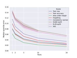
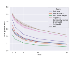
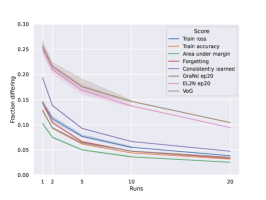
Figure 3: Variability in example difficulty scores due to sample size. Left and Center: Variability in ranking examples by their mean difficulty scores. Scores are averaged over a fixed number of runs (x-axis), and the median (Left) and 95% confidence interval (Center) of absolute rank change between two such sets of runs is shown (y-axis). Right: variability in 50% data splits found by thresholding mean difficulty scores. Number of runs that scores are averaged over (x-axis) is plotted against the fraction of examples that change classification between two such sets of runs (y-axis).

4.2 Correlation Between Scores

We next examine the degree to which different scores are related, and whether scores averaged over runs are more or less predictive of individual run scores and other mean scores. As scores generally have non-linear but monotonic relationships, we use Spearman (rank) correlation to better capture the full dependence between scores. Note that correlations between related quantities are expected to be strong: for example, Loss training, Accuracy training, and Area under margin are all functions of the model output, although they are not directly recoverable from one another.

Figure 4 shows the correlation between mean scores, which is high for most scores with the lowest at $\rho>0.6$ for Ensemble agreement (Carlini et al.,, 2019). Figure 4 (Center) also shows the reduction/increase in correlation when using means to predict individual runs instead of other mean. We find that all of these changes are negative, indicating that mean scores are less predictive of individual runs than other means, which is unsurprising given the high per-run variances observed in Figure 2. Note that the diagonal in Figure 4 (Center) is $\rho-1$, where $\rho$ is the correlation between the mean and individual runs of a given score.

Finally, Figure 4 (Right) shows the reduction/increase in correlation when using individual runs to predict other runs instead of mean scores. Note that the diagonal should be ignored since the score of an individual run is always perfectly correlated with itself—the diagonal in Figure 4 (Right) is simply the inverse of Figure 4 (Center), i.e. $1-\rho$. Positive values indicate that scores from an individual run are better predictors of another score than their averaged counterparts. Although most changes are negative, closely related scores such as Train loss and Train accuracy, Forgetting and Consistently learned, or GraNd and EL2N have a notable increase in correlation when considering individual runs. This indicates that these pairs of scores vary in similar ways from run to run, so that they are more predictive of one another in a given run than than their averaged counterparts.

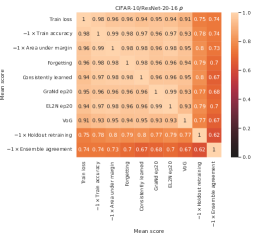
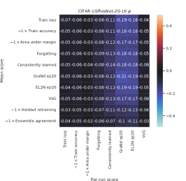
Figure 4: Spearman (rank) correlation between difficulty scores. To ensure positive correlations, scores are multiplied by $-1$ where required. Left: correlations between mean difficulty scores. All scores other than “Ensemble agreement” and “Holdout retraining” are averaged over 40 runs; the latter are pre-computed in Carlini et al., (2019), Center: difference in correlation when correlating mean scores (rows) with individual runs (columns), i.e. $\mathbb{E}_{Y}[Corr(\mathbb{E}_{X}[X],Y)]-Corr(\mathbb{E}_{X}[X],\mathbb{E}_{Y}[Y])$. Note that individual runs are not available for “Ensemble agreement” and “Holdout retraining” scores. Right: difference in correlation when correlating scores within individual runs scores, i.e. $\mathbb{E}_{X,Y}[Corr(X,Y)]-Corr(\mathbb{E}_{X}[X],Y)$.

To determine the dimensionality of the space which scores span, we conduct a principal component analysis (PCA) in Figure 5 to extract the top directions of variation and the amount of variance present in each direction. In the vein of the Spearman correlation used in Figure 4, we first apply a quantile transform to account for non-linear relationships among scores. We find that the first principal component (PCA 1) accounts for the majority of variation (about 85%), and is almost equally weighted across all scores. This suggests that PCA 1 represents a common notion of an example’s “difficulty” shared by all scores.

The remaining directions of variation seem to represent variation from specific scores, with Ensemble agreement, Holdout retraining, Forgetting, and VoG representing distinct directions that collectively capture about 10% of total variation. Note that this does not contradict findings in Hooker et al., (2019); Baldock et al., (2021); Carlini et al., (2019) that suggest difficulty is 2 dimensional, since these works also consider different train/test splits (which we omit).

We also consider whether a linear combination of scores can reduce per-run variation. Figure 5 (Right) plots the same ranking and thresholding analysis as Figure 3, but using PCA 1 as a score. We find a similar magnitude of variation as the average among the scores from Figure 3, which reinforces the observation that the variation outside of PCA 1 is independent between different scores.

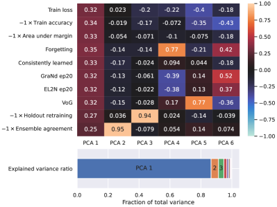
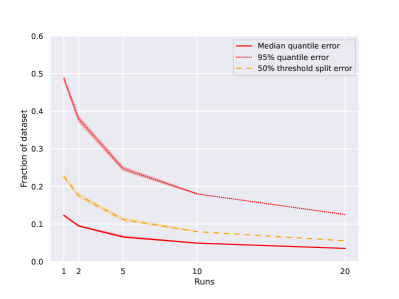
Figure 5: Principal component analysis of mean difficulty scores. All scores are first transformed to the normal distribution via quantile transform. Left: linear coefficients for top-6 principal components accounting for $>98\%$ of variation (heatmap top), and ratio of explained variance per component (stacked bars bottom). Right: variation in data splits by 50% threshold, median absolute rank error, and 95% confidence interval for ranks when using the top principal component as a score. This plot is analogous to Figure 3.

4.3 Effect of Inductive Bias

We examine the degree to which different model architectures, widths, and depths affect scores, and the degree to which such effects are distinguishable from the variation between runs. Inspired by computational genetics and the genome-wide association study in particular (Clarke et al.,, 2011), we run an independent two-sample test of difference of means for every example. This effectively ranks examples by their bias to variance ratio in per-run scores, where bias is the change in difficulty between two different models.

Figure 6 plots the statistical significance of differences in mean difficulty for a variety of different pairs of model architectures. We report the mean of the negative logarithm of $P$ values for all scores and/or all architecture pairs (equivalent to the geometric mean of $P$ values), with higher values corresponding to greater statistical significance. Unsurprisingly, in Figure 6 (Left) we find that scores that vary the least between runs Figure 2 tend to have higher statistical significance, such as Area under margin. Interestingly, although Loss training and Accuracy training are closely related to Area under margin, they have much lower significance likely because they lose more of the information from the model output. Among different architecture pairs in Figure 6 (Center), we find large architectural changes (e.g. ResNet versus VGG) lead to more significant differences than small changes (e.g. increasing ResNet depth). To investigate whether differences in model size (i.e. number of trainable parameters) can account for changes in example difficulty, we plot average $P$ value over all examples versus the size ratio between architecture pairs (Figure 6 Right). Although differences in model size correspond weakly to more significant differences in difficulty, there are also many pairs of similarly sized models which induce relatively significant changes in difficulty.

Finally, we show that a handful of the most significant examples can be used to fingerprint a model’s inductive bias. Figure 1 (Left) visualizes the examples with the most and least significant $P$ values (according to the geometric mean over all scores and model architecture pairs). The top examples most sensitive to inductive biases are visibly more difficult than the bottom examples with consistent difficulty. Scores from these examples are then used as features for identifying a model as either VGG-16 or ResNet-20, by fitting a logistic classifier (no regularization) to each type of score. Classifers are fit using scores from 20 runs, and evaluated on a separate set of 20 runs. Figure 1 (Right) shows that for most scores, the top 8 examples are sufficient to perfectly classify VGG-16/ResNet model architectures, reliably beating 8 random examples, whereas the bottom 8 examples perform no better than chance.

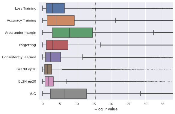
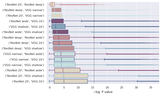
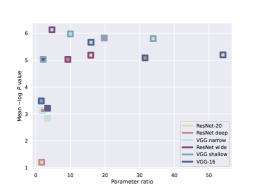
Figure 6: Distribution of $P$ values for unpaired t-tests for all scores and examples. $P$ values indicate the likelihood of the null hypothesis: namely that two populations of per-example difficulty scores from different inductive biases have the same mean. The negative log of the $P$ values is reported, with higher values corresponding to more statistically significant differences in means. The inductive biases compared are all pairs of models with different width, depth, and/or architecture (VGG/ResNet). Left and Center: $P$ value distribution by difficulty score or model architecture pairs. X-axis reports negative logarithm (higher values are more significant), with dotted line indicating a Bonferroni-corrected threshold of $p=0.01$. Right: Geometric mean of $P$ value over all examples and scores, versus relative difference in model capacity (ratio of number of trainable parameters).

5 Discussion

Despite appearing to be intuitive, the difficulty of an example is a rather nebulous concept that has thus far evaded systematic study. In this work, we establish that there is a common notion of difficulty among training examples, and that each example’s difficulty is affected to different degrees by randomness (from model initialization, SGD training noise, etc.) and the method/model used to score it. We find that scores have high variance over individual runs which is inconsistent from example to example, raising concerns over the error inherent in score estimates.

The high correlation between scores suggests a greater degree of interchangeability among scores than one might expect. This gives practitioners greater freedom in selecting scores, such as to replace a costly score like Feldman and Zhang, (2020) with a proxy as in Jiang et al., (2020), without requiring additional techniques as in Liu et al., (2021). This also tempers the advantages claimed by some scores as especially good predictors of other scores (Baldock et al.,, 2021; Agarwal et al.,, 2020).

As the majority (85%) of score variation among training examples lies in a single direction, we propose that this direction represents a common notion of “difficulty” measured by all scores. Based on this finding, we hypothesize that the additional directions of variation proposed by Hooker et al., (2019); Baldock et al., (2021); Carlini et al., (2019) also represent a second shared direction of variation measuring difficulty when an example is in the test set. It is unclear if the second dimension in Swayamdipta et al., (2020) (based on variance over training) is related to these two directions.

Lastly, we show that examples range from being model-independent to being strongly dependent on the inductive biases of a given model. The former examples allow scores to be compared between different models, whereas the latter can be used as lightweight features for classifying model architectures using a downstream method such as logistic regression. In our case, a simple statistical test for difference of means was sufficient to identify model-dependent examples. We note however, that there are methods from statistical genetics with greater statistical power (e.g. MTAG from Turley et al., (2018)), which could potentially find examples that are sensitive to much smaller differences in inductive biases. We leave the investigation of these methods for future work.

This research was enabled in part by compute resources provided by Mila (mila.quebec).

References

- Agarwal et al., (2020) Agarwal, C., D’souza, D., and Hooker, S. (2020). Estimating example difficulty using variance of gradients. arXiv preprint arXiv:2008.11600.
- Baldock et al., (2021) Baldock, R., Maennel, H., and Neyshabur, B. (2021). Deep learning through the lens of example difficulty. Advances in Neural Information Processing Systems, 34.
- Birodkar et al., (2019) Birodkar, V., Mobahi, H., and Bengio, S. (2019). Semantic redundancies in image-classification datasets: The 10% you don’t need. arXiv preprint arXiv:1901.11409.
- Carlini et al., (2019) Carlini, N., Erlingsson, U., and Papernot, N. (2019). Distribution density, tails, and outliers in machine learning: Metrics and applications. arXiv preprint arXiv:1910.13427.
- Clarke et al., (2011) Clarke, G. M., Anderson, C. A., Pettersson, F. H., Cardon, L. R., Morris, A. P., and Zondervan, K. T. (2011). Basic statistical analysis in genetic case-control studies. Nature protocols, 6(2):121–133.
- Dosovitskiy et al., (2021) Dosovitskiy, A., Beyer, L., Kolesnikov, A., Weissenborn, D., Zhai, X., Unterthiner, T., Dehghani, M., Minderer, M., Heigold, G., Gelly, S., Uszkoreit, J., and Houlsby, N. (2021). An image is worth 16x16 words: Transformers for image recognition at scale. In International Conference on Learning Representations.
- Feldman and Zhang, (2020) Feldman, V. and Zhang, C. (2020). What neural networks memorize and why: Discovering the long tail via influence estimation. Advances in Neural Information Processing Systems, 33:2881–2891.
- Hacohen et al., (2020) Hacohen, G., Choshen, L., and Weinshall, D. (2020). Let’s agree to agree: Neural networks share classification order on real datasets. In International Conference on Machine Learning, pages 3950–3960. PMLR.
- He et al., (2016) He, K., Zhang, X., Ren, S., and Sun, J. (2016). Deep residual learning for image recognition. In Proceedings of the IEEE conference on computer vision and pattern recognition, pages 770–778.
- Hooker et al., (2019) Hooker, S., Courville, A., Clark, G., Dauphin, Y., and Frome, A. (2019). What do compressed deep neural networks forget? arXiv preprint arXiv:1911.05248.
- Hooker et al., (2020) Hooker, S., Moorosi, N., Clark, G., Bengio, S., and Denton, E. (2020). Characterising bias in compressed models. arXiv preprint arXiv:2010.03058.
- (12) Jiang, A. H., Wong, D. L.-K., Zhou, G., Andersen, D. G., Dean, J., Ganger, G. R., Joshi, G., Kaminksy, M., Kozuch, M., Lipton, Z. C., et al. (2019a). Accelerating deep learning by focusing on the biggest losers. arXiv preprint arXiv:1910.00762.
- (13) Jiang, Y., Krishnan, D., Mobahi, H., and Bengio, S. (2019b). Predicting the generalization gap in deep networks with margin distributions. In International Conference on Learning Representations.
- Jiang et al., (2020) Jiang, Z., Zhang, C., Talwar, K., and Mozer, M. C. (2020). Characterizing structural regularities of labeled data in overparameterized models. arXiv preprint arXiv:2002.03206.
- Jin et al., (2022) Jin, T., Carbin, M., Roy, D., Frankle, J., and Dziugaite, G. K. (2022). Pruning’s effect on generalization through the lens of training and regularization. Advances in Neural Information Processing Systems, 35:37947–37961.
- Kalimeris et al., (2019) Kalimeris, D., Kaplun, G., Nakkiran, P., Edelman, B., Yang, T., Barak, B., and Zhang, H. (2019). Sgd on neural networks learns functions of increasing complexity. In Wallach, H., Larochelle, H., Beygelzimer, A., d'Alché-Buc, F., Fox, E., and Garnett, R., editors, Advances in Neural Information Processing Systems, volume 32. Curran Associates, Inc.
- Krizhevsky, (2009) Krizhevsky, A. (2009). Learning multiple layers of features from tiny images. Technical report.
- Liu et al., (2021) Liu, F., Lin, T., and Jaggi, M. (2021). Understanding memorization from the perspective of optimization via efficient influence estimation. arXiv preprint arXiv:2112.08798.
- Meding et al., (2021) Meding, K., Buschoff, L. M. S., Geirhos, R., and Wichmann, F. A. (2021). Trivial or impossible–dichotomous data difficulty masks model differences (on imagenet and beyond). arXiv preprint arXiv:2110.05922.
- Nohyun et al., (2023) Nohyun, K., Choi, H., and Chung, H. W. (2023). Data valuation without training of a model. In International Conference on Learning Representations.
- Northcutt et al., (2021) Northcutt, C., Jiang, L., and Chuang, I. (2021). Confident learning: Estimating uncertainty in dataset labels. Journal of Artificial Intelligence Research, 70:1373–1411.
- Paul et al., (2021) Paul, M., Ganguli, S., and Dziugaite, G. K. (2021). Deep learning on a data diet: Finding important examples early in training. Advances in Neural Information Processing Systems, 34.
- Pleiss et al., (2020) Pleiss, G., Zhang, T., Elenberg, E., and Weinberger, K. Q. (2020). Identifying mislabeled data using the area under the margin ranking. Advances in Neural Information Processing Systems, 33:17044–17056.
- Pruthi et al., (2020) Pruthi, G., Liu, F., Kale, S., and Sundararajan, M. (2020). Estimating training data influence by tracing gradient descent. In Larochelle, H., Ranzato, M., Hadsell, R., Balcan, M., and Lin, H., editors, Advances in Neural Information Processing Systems, volume 33, pages 19920–19930. Curran Associates, Inc.
- Siddiqui et al., (2022) Siddiqui, S. A., Rajkumar, N., Maharaj, T., Krueger, D., and Hooker, S. (2022). Metadata archaeology: Unearthing data subsets by leveraging training dynamics. arXiv preprint arXiv:2209.10015.
- Simonyan and Zisserman, (2015) Simonyan, K. and Zisserman, A. (2015). Very deep convolutional networks for large-scale image recognition. In 3rd International Conference on Learning Representations (ICLR 2015). Computational and Biological Learning Society.
- Sorscher et al., (2022) Sorscher, B., Geirhos, R., Shekhar, S., Ganguli, S., and Morcos, A. S. (2022). Beyond neural scaling laws: beating power law scaling via data pruning. arXiv preprint arXiv:2206.14486.
- Swayamdipta et al., (2020) Swayamdipta, S., Schwartz, R., Lourie, N., Wang, Y., Hajishirzi, H., Smith, N. A., and Choi, Y. (2020). Dataset cartography: Mapping and diagnosing datasets with training dynamics. In Proceedings of the 2020 Conference on Empirical Methods in Natural Language Processing (EMNLP), pages 9275–9293.
- Toneva et al., (2019) Toneva, M., Sordoni, A., des Combes, R. T., Trischler, A., Bengio, Y., and Gordon, G. J. (2019). An empirical study of example forgetting during deep neural network learning. In International Conference on Learning Representations.
- Turley et al., (2018) Turley, P., Walters, R. K., Maghzian, O., Okbay, A., Lee, J. J., Fontana, M. A., Nguyen-Viet, T. A., Wedow, R., Zacher, M., Furlotte, N. A., et al. (2018). Multi-trait analysis of genome-wide association summary statistics using mtag. Nature genetics, 50(2):229–237.
- Yang et al., (2023) Yang, Y., Gan, E., Dziugaite, G. K., and Mirzasoleiman, B. (2023). Identifying spurious biases early in training through the lens of simplicity bias. arXiv preprint arXiv:2305.18761.