Fluctuation of the largest eigenvalue of a Kernel Matrix with application in Graphon-based random graphs

Abstract.

In this article, we explore the spectral properties of general random kernel matrices $\left[\mathsf{K}(U_{i},U_{j})\right]_{1\leq i\neq j\leq n}$ from a Lipschitz kernel $\mathsf{K}$ with $n$ independent random variables $U_{1},U_{2},\ldots,U_{n}$ distributed uniformly over $[0,1]$. In particular we identify a dichotomy in the extreme eigenvalue of the kernel matrix, where, if the kernel $\mathsf{K}$ is degenerate, the largest eigenvalue of the kernel matrix (after proper normalization) converges weakly to a weighted sum of independent chi-squared random variables. In contrast, for non-degenerate kernels, it converges to a normal distribution extending and reinforcing earlier results from [39]. Further, we apply this result to show a dichotomy in the asymptotic behavior of extreme eigenvalues of $W$-random graphs, which are pivotal in modeling complex networks and analyzing large-scale graph behavior. These graphs are generated using a kernel $W$, termed as graphon, by connecting vertices $i$ and $j$ with probability $W(U_{i},U_{j})$. Our results show that for a Lipschitz graphon $W$, if the degree function is constant, the fluctuation of the largest eigenvalue (after proper normalization) converges to the weighted sum of independent chi-squared random variables and an independent normal distribution. Otherwise, it converges to a normal distribution.

1. Introduction

In recent years, the study of graph theory has gained significant momentum, owing to its applicability in diverse fields ranging from biology and physics to social sciences and computer networks [12, 45, 56, 14]. Many interesting properties of graphs are revealed by the extreme eigenvalues and eigenvectors of their adjacency matrices. To mention some, we refer the readers to the books [15, 21] for a general discussion on spectral graph theory, the survey article [32] for the connection between eigenvalues and expansion properties of graphs, and the articles [46, 47, 48, 53, 54, 55] on the applications of eigenvalues and eigenvectors in various algorithms, i.e., combinatorial optimization, spectral partitioning and clustering. The Erdös–Rényi graphs and random $d$-regular graphs serve as the two prototypical models for random graphs, and their extreme eigenvalues have been extensively studied [36, 62, 40, 1, 59, 23, 29, 35, 41, 34, 51, 58, 28, 6, 22, 25, 26, 13].

In this paper, we study the extreme eigenvalues of random graphs generated from graphons, which are generalizations of Erdös–Rényi graphs. Recall that a graphon, denoted as $W$, is a symmetric, measurable function that offers a powerful framework for understanding the limiting behavior of large graph sequences, see [44, 43]. A graphon $W$ gives rise to a way of generating random graphs. This construction leads to the $W$-random graphs, which serve as a fundamental tool for modeling and analyzing the behavior of large-scale networks. These graphs are generated using a graphon $W$ by first creating an $n\times n$ random kernel matrix $\left[W(U_{i},U_{j})\right]_{1\leq i\neq j\leq n}$ (we do not allow self-loops) using $n$ independent numbers $U_{1},U_{2},\cdots,U_{n}$ uniformly distributed over $[0,1]$. This random kernel matrix then gives rise to a random simple graph: connecting nodes $i$ and $j$ with probability $W(U_{i},U_{j})$. The focus of this paper is the spectral analysis of the random kernel matrices, and the $W$-random graphs.

Our first main result concerns about the extreme eigenvalues of random kernel matrices formed from a general integral kernel $\mathsf{K}$ (graphons are special examples). The spectral properties of such random kernel matrices have been studied in the pioneer work [39]. It is proved that the $L_{2}$ distance between the ordered spectrum of the random kernel matrices $\{\mathsf{K}(U_{i},U_{j})\}_{1\leq i\neq j\leq n}$ and the ordered spectrum of $\mathsf{K}$ tends to zero. Under certain technical conditions, a distributional limit theorems for the eigenvalues of the random kernel matrices are also obtained. However, the conditions in [39] are not easy to check unless $\mathsf{K}$ is of finite rank, see Remark 2.3. Moreover the distributional limit theorem in [39] is trivial (the limit is a normal with variance $0$) when the kernel $\mathsf{K}$ is degenerate, namely the eigenfunction corresponding to the largest eigenvalue is a constant function. Notice that this notion of degeneracy is related to the notion of degenerate kernels appearing in the study of $U$-statistics (see [60]).

We revisit the spectral problem of random kernel matrices $\{\mathsf{K}(U_{i},U_{j})\}_{1\leq i\neq j\leq n}$ and extend the distributional limit theorems in [39] in two ways. First we identify a simple condition that as long as the kernel is Lipschitz (probably can be further relaxed to piecewise lipschitz), the largest eigenvalue converges to a normal random variable. Secondly, in the degenerate case, if we further rescale by a factor $\sqrt{n}$, the largest eigenvalue converges to a generalized chi-squared distribution. We obtain an explicit characterization of it in terms of the spectrum of $\mathsf{K}$. This leads to Theorem 2.1 showing a dichotomy in the extreme eigenvalues of random kernel matrices coming from a Lipschitz kernel. Specifically, if the kernel is degenerate, the largest eigenvalue converges weakly to a weighted (possibly infinite) sum of independent chi-squared random variables. In contrast, for non-degenerate kernels, it converges to a normal distribution.

To study the spectra of random kernel matrices, we first derive a master equation (4.6), which characterizes their largest eigenvalues. Such master equation has been used intensively in random matrix theory to study random perturbation of low rank matrices, see [2, 3, 33, 8, 7, 57]. However, our case is not of low rank, instead we need to invert a full rank matrix. To address this challenge, we implement a finite rank approximation, which effectively transforms our problem into one of finite rank perturbation. This can be analyzed using the Woodbury formula. A crucial aspect of our approach is to establish that the error introduced by the finite rank approximation is minor and does not impact the distribution limit theorems we aim to prove. This is particularly pertinent in the degenerate case, where the fluctuation of the largest eigenvalue is of order $O(1)$, contrasting with the $O(\sqrt{n})$ order typically expected. This is done through detailed resolvent expansion analyses, and the error can be made arbitrarily small by selecting a sufficiently high rank for our approximation.

Our second main result concerns about the extreme eigenvalues of $W$-random graphs from a graphon $W$. As an intermediate step, we study the adjacency matrix $\bm{A}_{n}$ conditioning on the connectivity probability matrix $\bm{W}_{n}=\{W(U_{i},U_{j})\}_{1\leq i\neq j\leq n}$. This can be viewed as an inhomogeneous Erdős-Rényi model, where edges are added independently among the $n$ vertices with varying probabilities $p_{ij}=W(U_{i},U_{j})$. Many popular random graph models arise as special cases of inhomogeneous Erdős-Rényi model such as random graphs with given expected degrees [20] and stochastic block models [31].

The adjacency matrix $\bm{A}_{n}$ decomposes as the sum of the centered adjacency matrix and the connectivity probability matrix:

$$\bm{A}_{n}=\left(\bm{A}_{n}-\mathbb{E}\left[\bm{A}_{n}\middle|U_{1},\ldots,U_{n}\right]\right)+\mathbb{E}\left[\bm{A}_{n}\middle|U_{1},\ldots,U_{n}\right]=(\bm{A}_{n}-\bm{W}_{n})+\bm{W}_{n}.$$ (1.1)

The empirical eigenvalue distributions and the behavior of extreme eigenvalues of centered adjacency matrices in inhomogeneous Erdős–Rényi graphs have been the subject of extensive study, as detailed in [63, 10, 9]. Some of these findings also cover sparse graph regimes. In the context of the uncentered adjacency matrix $\bm{A}_{n}$, it has been established [19] that in sparse settings the empirical eigenvalue distributions converge towards a deterministic measure. The fluctuations of the extreme eigenvalues of adjacency matrix $\bm{A}_{n}$ have been studied in a recent work [18]. It has been proven that if the connectivity probability matrix is of finite rank $k$, then the joint distribution of the $k$ largest eigenvalues of $\bm{A}_{n}$ converge jointly to a multivariate Gaussian law. When the connectivity probability matrix is constant, these results coincide with the established fluctuations of the maximum eigenvalue in homogeneous Erdős–Rényi graphs, [23]. Our result, 4.6 extends these results to the general infinite rank connectivity probability matrix constructed from Lipschitz graphons. This together with Theorem 2.1 leads to our second main result, Theorem 2.2 regarding $W$-random graphs from a Lipschitz graphon. If the graphon’s degree function is constant, the fluctuation of the largest eigenvalue converges to the generalized chi-squared distribution. Otherwise, it converges to a normal distribution.

When the connectivity matrix $\bm{W}_{n}$ in (1.1) is of finite rank, the extreme eigenvalues of (1.1) can be studied as a spiked Wigner matrix model, which has been intensively studied in the past decades [24, 5, 18, 27, 4, 17, 37, 38]. Full rank deformation of the Gaussian unitary matrix and Wigner matrices have also been studied in [16, 42]. In our case, it turns out the connectivity probability matrix $\bm{W}_{n}$ is dominant (it is of full rank). This prompts us to consider the adjacency matrix $\bm{A}_{n}$ as a small perturbation of $\bm{W}_{n}$. Similarly to the study of the random kernel matrix, we again derive a master equation (4.27) which characterizes the largest eigenvalue of $\bm{A}_{n}$. We then analyze the master equation by a perturbation argument, and express the largest eigenvalue in terms of the kernel matrix $\bm{W}_{n}$. Using the estimates on the eigenvalue and eigenvectors of the kernel matrix from the first part, we finally show that the difference between the largest eigenvalue of $\bm{A}_{n}$ and $\bm{W}_{n}$ has a Gaussian fluctuation, independent of the contribution of $\bm{W}_{n}$ conditional on the node information $U_{1},\ldots,U_{n}$. The decomposition in (1.1) along with a standard application of Weyl’s inequality shows that in non-degenerate case the difference $\bm{A}_{n}-\bm{W}_{n}$ has negligible contribution. On the other hand, in the degenerate case, the fluctuation of $\lambda_{1}(\bm{A}_{n})$ follows from the contribution of $\lambda_{1}(\bm{W}_{n})$ and the independent Gaussian contribution of $\lambda_{1}(\bm{A}_{n})-\lambda_{1}(\bm{W}_{n})$.

The remaining part of the paper is organized as following: the main results of the paper Theorem 2.1 and Theorem 2.2 are stated in Section 2. We validate the main results through numerical experiments in LABEL:sec:simulations. and outline the proof of our main results in Section 4. We collect some preliminary results on kernel matrices in Section 5 and their proofs are deferred to Appendix A and Appendix B. Proof details for Theorem 2.1 are presented in Section 6 and Appendix C. Proof details for Theorem 2.2 are given in Section 7 and Appendix D. We collect some useful facts on the spectrum of self-adjoint compact operators in Appendix E. All the appendices are presented in the supplementary material.

1.1. Notations

In this section we collect common notations that are used throughout the article. We use $\stackrel{{\scriptstyle P}}{{\to}}$ and $\stackrel{{\scriptstyle D}}{{\to}}$ to denote convergences in probability and distribution respectively. A random variable $X_{n}=O_{p}(a_{n})$ implies that for all $\varepsilon>0$ there exists $M_{\varepsilon}>0$ such that, $\mathbb{P}\left[\left|X_{n}/a_{n}\right|>M_{\varepsilon}\right]\leq\varepsilon\text{ for all large enough }n$. The notations $a\lesssim_{\theta}b$ and $a=O_{\theta}(b)$ are used to say $a\leq C_{\theta}b$ for some constant $C_{\theta}>0$ depending on a parameter $\theta$. A similar definition applies to $a\gtrsim_{\theta}b$. A random variable $X_{n}=o_{p}(a_{n})$ implies the ratio $X_{n}/a_{n}$ converges in probability to $0$ as $n\rightarrow\infty$ and in the deterministic case $a_{n}=o(b_{n})$ implies the ratio $a_{n}/b_{n}\rightarrow 0$ as $n\rightarrow\infty$. For a kernel $f$ we use the notation $\sigma(f)$ to denote the spectrum of $f$, that is the set of eigenvalues of the integral operator $T_{f}$, $T_{f}(g)(x)=\int f(x,y)g(y)\mathrm{d}y$. To denote the Gaussian distribution with mean $\mu$ and variance $\sigma^{2}$ the notation $\mathcal{N}(\mu,\sigma^{2})$ is used and to denote Uniform distribution on $[0,1]$ the notation $\text{Unif}\ [0,1]$ is used. We use the notation $C$ to denote a universal positive constant.

2. Main Results

We make the following assumptions on the kernel matrix. The first one requires that the kernel is Lipschitz continuous, and the second one requires that there is a spectral gap.

Assumption 2.1.

We assume the kernel $\mathsf{K}:[0,1]^{2}\mapsto\mathbb{R}$ has the following properties:

1. $|\mathsf{K}|\leq 1$ and $\mathsf{K}$ is Lipschitz continuous with Lipschitz constant $L_{\mathsf{K}}>0$.

2. Enumerate the eigenvalues of $\mathsf{K}$ as $\lambda_{1}(\mathsf{K})\geq\lambda_{2}(\mathsf{K})\geq\cdots\geq 0$ and $\lambda_{1}^{\prime}(\mathsf{K})\leq\lambda_{2}^{\prime}(\mathsf{K})\leq\cdots\leq 0$, $\phi_{j}$ and $\phi_{j}^{\prime}$ being the orthonormal eigenfunctions corresponding to the eigenvalues $\lambda_{j}(\mathsf{K})$ and $\lambda_{j}^{\prime}(\mathsf{K})$ respectively. Then,

   $$\left|\lambda_{1}(\mathsf{K})-\lambda_{2}(\mathsf{K})\right|>0.$$

In the following we formally introduce the notion of degeneracy of a kernel $\mathsf{K}$. The behavior of the largest eigenvalue of the random kernel matrix depends on the degeneracy of the kernel.

Definition 2.1.

Let $\mathsf{K}$ be a kernel with $\phi_{1}$ the eigenfunction corresponding to the largest eigenvalue. Then $\mathsf{K}$ is called degenerate if $\phi_{1}$ is almost surely constant.

Notice that by Definition 2.1 a graphon $W$ is degenerate if and only if the degree function of $W$ is almost surely constant. In other words, a graphon is degenerate if and only if it is degree regular. A similar notion of degeneracy has been studied with respect to small subgraph counts in [30] and [11].

Our first main result is on the extreme eigenvalues of the $n\times n$ kernel matrix $\bm{\mathsf{K}}_{n}$ constructed from $\mathsf{K}$,

$$(\bm{\mathsf{K}}_{n})_{i,j}=\mathsf{K}(U_{i},U_{j})\delta_{i\neq j},\quad 1\leq i,j\leq n,$$ (2.1)

where $\bm{U}_{n}:=(U_{1},\ldots,U_{n})\overset{i.i.d.}{\sim}\text{Unif}[0,1]$. We discover a dichotomous behavior of the extreme eigenvalues of the kernel matrix $\bm{\mathsf{K}}_{n}$.

Theorem 2.1.

Adopt 2.1, and construct the kernel matrix $\bm{\mathsf{K}}_{n}$ as in (2.1). We denote the largest eigenvalue of $\bm{\mathsf{K}}_{n}$ as $\lambda_{1}(\bm{\mathsf{K}}_{n})$, then

1. If $\mathsf{K}$ is not degenerate, namely $\phi_{1}$ is not a constant function, then

   $$\sqrt{n}\bigg{(}\frac{\lambda_{1}(\bm{\mathsf{K}}_{n})}{n}-\lambda_{1}(\mathsf{K})\bigg{)}\stackrel{{\scriptstyle D}}{{\to}}\mathcal{N}\left(0,\lambda_{1}(\mathsf{K})^{2}\operatorname{Var}\left(\phi_{1}^{2}(U)\right)\right),$$ (2.2)

   where $U{\sim}\emph{Unif}[0,1]$.

2. If $\mathsf{K}$ is degenerate, namely $\phi_{1}$ is a constant function, then

   $$\lambda_{1}(\bm{\mathsf{K}}_{n})-(n-1)\lambda_{1}(\mathsf{K})\stackrel{{\scriptstyle D}}{{\to}}\zeta_{\infty}$$

   where

   $$\zeta_{\infty}:=\sum_{\lambda\in\sigma(\mathsf{K})\backslash\{\lambda_{1}(\mathsf{K})\}}\frac{\lambda_{1}(\mathsf{K})\lambda}{\lambda_{1}(\mathsf{K})-\lambda}(Z_{\lambda}^{2}-1)+\sum_{\lambda\in\sigma(\mathsf{K})\backslash\{\lambda_{1}(\mathsf{K})\}}\frac{\lambda^{2}}{\lambda_{1}(\mathsf{K})-\lambda},$$ (2.3)

   and $\{Z_{\lambda}:\lambda\in\sigma(\mathsf{K})\}$ are generated independently from the standard normal distribution.

Notice that the above Theorem holds true whenever the kernel $\mathsf{K}$ satisfies Assumption 2.1 and the matrix $\bm{\mathsf{K}}_{n}$ has zero as it’s diagonal elements. The result can be easily modified whenever the diagonal entries are given by $\mathsf{K}(U_{i},U_{i})$ for all $1\leq i\leq n$.

Corollary 2.1.

Adopt Assumption 2.1, and consider the kernel matrix $\bm{\mathsf{K}}_{n}=(K(U_{i},U_{j}))_{i,j=1}^{n}$. Then for the largest eigenvalue $\lambda_{1}(\bm{\mathsf{K}}_{n})$,

1. If $\mathsf{K}$ is not degenerate, namely $\phi_{1}$ is not a constant function, then

   $$\sqrt{n}\bigg{(}\frac{\lambda_{1}(\bm{\mathsf{K}}_{n})}{n}-\lambda_{1}(\mathsf{K})\bigg{)}\stackrel{{\scriptstyle D}}{{\to}}\mathcal{N}\left(0,\lambda_{1}(\mathsf{K})^{2}\operatorname{Var}\left(\phi_{1}^{2}(U)\right)\right),$$

   where $U{\sim}\emph{Unif}[0,1]$.

2. If $\mathsf{K}$ is degenerate, namely $\phi_{1}$ is a constant function and $\sum_{\lambda\in\sigma(\mathsf{K})}|\lambda|<\infty$, then

   $$\lambda_{1}(\bm{\mathsf{K}}_{n})-(n-1)\lambda_{1}(\mathsf{K})\stackrel{{\scriptstyle D}}{{\to}}\sum_{\lambda\in\sigma(\mathsf{K})\backslash\{\lambda_{1}(\mathsf{K})\}}\frac{\lambda_{1}(\mathsf{K})\lambda}{\lambda_{1}(\mathsf{K})-\lambda}Z_{\lambda}^{2}$$

   where $\{Z_{\lambda}:\lambda\in\sigma(\mathsf{K})\}$ are generated independently from the standard normal distribution.

In contrast to Theorem 2.1(2) the additional assumption on summability of eigenvalues of the operator $\mathsf{K}$ in Corollary 2.1(2) is needed to ensure existence of the asymptotic distribution.

Remark 2.1.

We remark that if $\mathsf{K}$ is degenerate, namely $\phi_{1}$ is a constant function, then $\operatorname{Var}(\phi_{1}^{2}(U))=0$ for $U{\sim}\text{Unif}[0,1]$, and the righthand side of (2.2) degenerates. $\zeta_{\infty}$ in (2.3) degenerates, namely $\zeta_{\infty}\equiv 0$, only if $\lambda=0$ for all $\lambda\in\sigma(\mathsf{K})\backslash\{\lambda_{1}(\mathsf{K})\}$. In this case $\mathsf{K}=\lambda_{1}(\mathsf{K})\bm{1}$ is a constant kernel.

Remark 2.2.

Our result can be extended to other eigenvalues of $\bm{\mathsf{K}}_{n}$. For $t>1$, denote $\lambda_{t}(\bm{\mathsf{K}}_{n})$ as the $t$-th largest eigenvalue of $\bm{\mathsf{K}}_{n}$. However, in this case the $t$-th eigenfunction $\phi_{t}$ can not be a constant function. We will not have a dichotomy as in Theorem 2.1. Instead, we will always have the convergence to the normal distribution: If $|\lambda_{t}(\mathsf{K})-\lambda_{t-1}(\mathsf{K})|,|\lambda_{t}(\mathsf{K})-\lambda_{t+1}(\mathsf{K})|>0$, then we will have

$$\sqrt{n}\bigg{(}\frac{\lambda_{t}(\bm{\mathsf{K}}_{n})}{n}-\lambda_{t}(\mathsf{K})\bigg{)}\stackrel{{\scriptstyle D}}{{\to}}\mathcal{N}\left(0,\lambda_{t}(\mathsf{K})^{2}\operatorname{Var}\left(\phi_{t}^{2}(U)\right)\right).$$

Remark 2.3.

The convergence to the normal distribution (2.2) has been proven in [39, Theorem 5.1] for all eigenvalues under the following assumptions: there exists a sequence $R_{n}\rightarrow\infty$ such that

$$\sum_{|r|>R_{n}}\lambda_{r}^{2}(\mathsf{K})=o(n^{-1})$$ (2.4)

and

$$\sum_{|r|\leq R_{n},|s|\leq R_{n}}\int_{0}^{1}\phi_{r}^{2}\phi_{s}^{2}\mathrm{d}x\sum_{|r|\leq R_{n},|s|\leq R_{n}}(\lambda_{r}(\mathsf{K})^{2}+\lambda_{s}(\mathsf{K})^{2})\int_{0}^{1}\phi_{r}^{2}\phi_{s}^{2}\mathrm{d}x=o(n).$$ (2.5)

The conditions (2.4) and (2.5) are not easy to check. Our main result Theorem 2.1 only requires that $\mathsf{K}$ is Lipschitz, which is easier to check. We remark that Lipschitz kernels in general does not satisfy the assumptions (2.4) and (2.5). Since for Lipschitz kernels, the eigenvalues decay like $1/n^{3/2+}$ [49, Section 4], so we can take $R_{n}=\sqrt{n}$ in the (2.4). Then in (2.5), if the eigenvector integrals are atleast $O(1)$, then the lefthand side of (2.5) simplifies

$$\phantom{{}={}}\sum_{|r|\leq R_{n},|s|\leq R_{n}}\int_{0}^{1}\phi_{r}^{2}\phi_{s}^{2}\mathrm{d}x\sum_{|r|\leq R_{n},|s|\leq R_{n}}(\lambda_{r}^{2}+\lambda_{s}^{2})\int_{0}^{1}\phi_{r}^{2}\phi_{s}^{2}\mathrm{d}x$$

$$\asymp\sum_{|r|\leq R_{n},|s|\leq R_{n}}1\sum_{|r|\leq R_{n},|s|\leq R_{n}}(\frac{1}{r^{3}}+\frac{1}{s^{3}})\asymp R_{n}^{3}=n^{3/2}.$$

This fails the assumption (2.5). In 2.1, we assume that $\mathsf{K}$ is Lipschitz, which can possibly be weakend to piecewise Lipschitz, or even piecewise Hölder continuous. But we will pursue it in the future work.

Remark 2.4.

More generally, we can consider any probability space $(\mathbb{R},\mathcal{B},\mu)$, where $\mathcal{B}$ is the Borel sigma algebra on $\mathbb{R}$ and $\mu$ is a probability measure on $\mathbb{R}$. Let $\mathsf{H}:\Omega^{2}\mapsto\mathbb{R}$ be a symmetric kernel, that is, a measurable function symmetric in its two entries. Let $\bm{X}_{n}=(X_{1},X_{2},\cdots,X_{n})\overset{i.i.d.}{\sim}\mu$, and we can construct the following random matrix,

$$(\bm{\mathsf{H}}_{n})_{i,j}=\mathsf{H}(X_{i},X_{j})\delta_{i\neq j},\quad 1\leq i,j\leq n.$$

Our result Theorem 2.1 gives fluctuation of the largest eigenvalue of $\bm{\mathsf{H}}_{n}$. Denote the cumulative density function of $\mu$ as $F_{\mu}$, and its functional inverse as $F_{\mu}^{-1}$, then $F_{\mu}^{-1}(U_{i})$ has the same law as $X_{i}$, where $U_{1},U_{2},\cdots,U_{n}$ are i.i.d. uniform distributed on $[0,1]$. Denote the pull back kernel under $F_{\mu}^{-1}$ as

$$\mathsf{K}(\cdot,\cdot)=\mathsf{H}(F_{\mu}^{-1}(\cdot),F_{\mu}^{-1}(\cdot)),$$ (2.6)

and the corresponding random kernel matrix

$$(\bm{\mathsf{K}}_{n})_{i,j}=\mathsf{K}(U_{i},U_{j})\delta_{i\neq j}=\mathsf{H}(F_{\mu}^{-1}(U_{i}),F_{\mu}^{-1}(U_{j}))\delta_{i\neq j},\quad 1\leq i,j\leq n.$$

Then $\bm{\mathsf{K}}_{n}$ has the same law as $\bm{\mathsf{H}}_{n}$, and Theorem 2.1 holds for $\bm{\mathsf{H}}_{n}$, provided that $\mathsf{K}$ constructed in (2.6) satisfies (2.1).

Our second main result concerns the largest eigenvalue of the adjacency matrix coming from a graphon $W$. Note that the graphon $W$ can be considered as a kernel and thus we assume that $W$ satisfies 2.1. We generate $U_{1},\ldots,U_{n}$ generated independently from $U[0,1]$. Then we consider an adjacency matrix $\bm{A}_{n}$ defined as,

$$\bm{A}_{n}(i,j)\sim\text{Ber}(W(U_{i},U_{j})),1\leq i<j\leq n$$ (2.7)

In this section we consider the fluctuation of the eigenvalues of $\bm{A}_{n}$, in particular the largest eigenvalue $\lambda_{1}(\bm{A}_{n})$.

Theorem 2.2.

Fix a graphon $W$ satisfying 2.1, denote its largest eigenvalue as $\lambda_{1}(W)$ and the associated eigenfunction $\phi_{1}$. We consider the adjacency matrix $\bm{A}_{n}$ corresponding to the graphon $W$ as in (2.7), and denote its largest eigenvalue as $\lambda_{1}(\bm{A}_{n})$, then

1. If the degree function of $W$ is not a constant, namely $\phi_{1}$ is not a constant function, then

   $$\sqrt{n}\bigg{(}\frac{\lambda_{1}(\bm{A}_{n})}{n}-\lambda_{1}(W)\bigg{)}\stackrel{{\scriptstyle D}}{{\to}}\mathcal{N}\left(0,\lambda_{1}(W)^{2}\operatorname{Var}\left(\phi_{1}^{2}(U)\right)\right),$$

   where $U{\sim}\emph{Unif}[0,1]$.

2. If the degree function of $W$ is a constant, namely $\phi_{1}$ is a constant function, then

   $$\lambda_{1}(\bm{A}_{n})-(n-1)\lambda_{1}(W)\stackrel{{\scriptstyle D}}{{\to}}\zeta_{\infty}+\mathcal{N}(\alpha,\sigma^{2})$$ (2.8)

   where

   $$\zeta_{\infty}:=\sum_{\lambda\in\sigma(W)\backslash\{\lambda_{1}(W)\}}\frac{\lambda_{1}(W)\lambda}{\lambda_{1}(W)-\lambda}(Z_{\lambda}^{2}-1)+\sum_{\lambda\in\sigma(W)\backslash\{\lambda_{1}(W)\}}\frac{\lambda^{2}}{\lambda_{1}(W)-\lambda},$$

   and $\{Z_{\lambda}:\lambda\in\sigma(W)\}$ are generated independently from the standard normal distribution, and $\mathcal{N}(\alpha,\sigma^{2})$ represent an independent normal distribution with mean $\alpha$ and variance $\sigma^{2}$ given by,

   $$\alpha=\frac{1}{\lambda_{1}(W)}\int\frac{\phi_{1}^{2}(x)+\phi_{1}^{2}(y)}{2}W(x,y)(1-W(x,y))\mathrm{d}x\mathrm{d}y,$$

   $$\sigma^{2}=2\int\phi_{1}^{2}(x)\phi_{1}^{2}(y)W(x,y)(1-W(x,y))\mathrm{d}x\mathrm{d}y$$

Remark 2.5.

When the graphon $W$ has constant degree profile, the largest eigenvalue of the adjacency matrix fluctuates on the scale $\Omega(1)$. When the graphon $W$ has irregular degree profile, the largest eigenvalue fluctuates on a much larger scale, $\Omega(\sqrt{n})$.

Remark 2.6.

Our result can be extended to other eigenvalues of $\bm{A}_{n}$. Once again for $t>1$, denote $\lambda_{t}(\bm{A}_{n})$ as the $t$-th largest eigenvalue of $\bm{A}_{n}$. However, in this case we will not have a dichotomy as in Theorem 2.2. Instead, we will always have the convergence to the normal distribution: If $|\lambda_{t}(W)-\lambda_{t-1}(W)|,|\lambda_{t}(W)-\lambda_{t+1}(W)|>0$, then we will have

$$\sqrt{n}\bigg{(}\frac{\lambda_{t}(\bm{A}_{n})}{n}-\lambda_{t}(W)\bigg{)}\stackrel{{\scriptstyle D}}{{\to}}\mathcal{N}\left(0,\lambda_{t}(W)^{2}\operatorname{Var}\left(\phi_{t}^{2}(U)\right)\right),$$

where $U{\sim}\mathrm{Unif}[0,1]$.

Remark 2.7.

A similar dichotomy of distributional convergence is also present for motif counts in random graphs generated as in (2.7). In particular, [30] extended the notion of edge-regularity to clique-regularity and showed that if a Graphon $W$ is regular with respect to a clique $K_{r}$ then the asymptotic distribution of $K_{r}$ counts in the random graph in $\eqref{eq:defAn}$ has a structure similar to (2.8) with a centered Gaussian and a Non-Gaussian component, where the non-Gaussian component is a weighted sum of independent chi-squared random variables with the weights related to the spectrum of a graphon derived from $W$. On the other hand, for $K_{r}$-irregular graphons, we get the familiar gaussian convergence. This result was further extended for general subgraphs by [11], who extended the notion of clique regularity to general subgraph regularity and showed a similar dichotomous asymptotic distribution.

3. Simulations

In this section we validate the asymptotic distributions from Theorem 2.1 and Theorem 2.2. In particular we construct example of Graphons (which also acts as kernels) satisfying Assumption 2.1 and the conditions of Theorems 2.1 and 2.2. Define, $\phi_{1}(x)=1$, $\phi_{2}(x)=\sqrt{3}(2x-1)$, $\phi_{3}(x)=\sqrt{5}(6x^{2}-6x+1)$ and $\phi_{4}(x)=\sqrt{7}\left(20x^{3}-30x^{2}+12x-1\right)$. Notice that $\phi_{i},1\leq i\leq 4$ are the first four “Shifted” Legendre Polynomial. By definition it is easy to notice that the collection $\{\phi_{i},1\leq i\leq 5\}\in L^{2}[0,1]$ and are orthonormal. Now we define the graphons as follows,

$$W_{1}(x,y)=\frac{1}{2}\phi_{2}(x)\phi_{2}(y)+\frac{1}{9}\phi_{3}(x)\phi_{3}(y)+\frac{1}{30}\phi_{4}(x)\phi_{4}(y),$$

and

$$W_{2}(x,y)=\frac{1}{5}\phi_{1}(x)\phi_{1}(y)+\frac{1}{9}\phi_{2}(x)\phi_{2}(y)+\frac{1}{30}\phi_{3}(x)\phi_{3}(y).$$

Notice that by construction $W_{1}$ and $W_{2}$ satisfies assumption 2.1 and $W_{2}$ has constant largest eigenfunction, while for $W_{1}$ the largest eigenfunction is non-constant.

Largest Eigenvalue of Kernel Matrix:

For $U_{1},\ldots,U_{n}$ generated randomly from $\mathrm{Unif}[0,1]$ distribution we consider the asymptotic distribution of largest eigenvalue of the kernel matrices constructed using $W_{1}$ and $W_{2}$ as in (2.1). For $W_{1}$ and $W_{2}$ we consider $n=1000$ and $n=100$ respectively, and repeat the experiment $500$ times to get repeated samples of the largest eigenvalue and construct histogram of the properly scaled samples (according to Theorem 2.1). We consider the asymptotic distribution from Theorem 2.1 and generate $10^{5}$ samples from it to provide a histogram. The comparison between sample distribution and asymptotic distribution is provided in Figure 1. The comprision presented in Figures 1(a) and 1(b) validates the asymptotic distribution presented in Theorem 2.1.

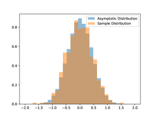
(a) Kernel Matrix with $W_{1}$.

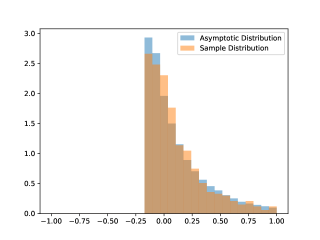
(b) Kernel Matrix with $W_{2}$.

Figure 1. Sample and Asymptotic Distribution of Largest Eigenvalue of Kernel Matrices.

Largest Eigenvalue of Adjacency Matrix:

Here we once again generate $U_{1},\ldots,U_{n}$ randomly from $\mathrm{Unif}[0,1]$ and construct Adjacency Matrix using the Graphon $W_{1}$ and $W_{2}$ following (2.7). Once again as above we consider $n=1000$ and $n=100$ for $W_{1}$ and $W_{2}$ respectively, and calculate the largest eigenvalue of the Adjacency matrix. We repeat the experiment $500$ times to have $500$ sample for the largest eigenvalue and follow the scalings from Theorem 2.2 to provide the histogram of the samples. To compare with the asymptotic distribution we once again generate $10^{5}$ samples from the asymptotic distribution and provide histogram using the samples. The comparision between sample and asymptotic distribution is provided in Figure 2, in particular the asymptotic distribution presented in Theorem 2.2 is validated by the comparison from Figures 2(a) and 2(b).

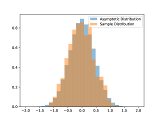
(a) Adjacency Matrix with $W_{1}$.

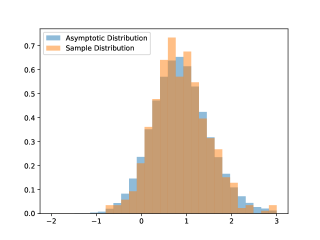
(b) Adjacency Matrix with $W_{2}$.

Figure 2. Sample and Asymptotic Distribution of Largest Eigenvalue of Adjacency Matrices.

4. Proof Outline

4.1. Proof of random kernel matrix limit

We recall the notations and assumptions on the kernel $\mathsf{K}$ from assumption 2.1. Since $\mathsf{K}$ is a self-adjoint integral operator (which is compact), we have the expansion,

$$\mathsf{K}(x,y)=\sum_{j=1}^{\infty}\lambda_{j}(\mathsf{K})\phi_{j}(x)\phi_{j}(y)+\sum_{j=1}^{\infty}\lambda_{j}^{\prime}(\mathsf{K})\phi_{j}^{\prime}(x)\phi_{j}^{\prime}(y)$$ (4.1)

where the equality holds in $L_{2}$ sense. In this section we study the eigenvalues of the $n\times n$ kernel matrix $\bm{\mathsf{K}}_{n}$ as,

$$(\bm{\mathsf{K}}_{n})_{i,j}=\mathsf{K}(U_{i},U_{j})\delta_{i\neq j},\quad 1\leq i,j\leq n,$$ (4.2)

where $\bm{U}_{n}:=(U_{1},\ldots,U_{n})\overset{i.i.d.}{\sim}\text{Unif}[0,1]$. Thanks to the decomposition (4.1), we can rewrite (4.2) as

$$\bm{\mathsf{K}}_{n}=\sum_{j=1}^{\infty}\lambda_{j}(\mathsf{K})\left(\Phi_{j}(\bm{U}_{n})\Phi_{j}(\bm{U}_{n})^{\top}-\bm{D}_{n,j}\right)+\sum_{j=1}^{\infty}\lambda_{j}^{\prime}(\mathsf{K})\left(\Phi_{j}^{\prime}(\bm{U}_{n})\Phi_{j}^{\prime}(\bm{U}_{n})^{\top}-\bm{D}_{n,j}^{\prime}\right)$$

where $\Phi_{j}(\bm{U}_{n}):=(\phi_{j}(U_{1}),\cdots,\phi_{j}(U_{n}))$, $\bm{D}_{n,j}:=\operatorname{diag}(\phi_{j}^{2}(U_{1}),\cdots,\phi_{j}^{2}(U_{n}))$ and $\Phi_{j}^{\prime}(\bm{U}_{n})$, $\bm{D}_{n,j}^{\prime}$ are defined similarly through $\phi_{j}^{\prime}$ and the equality is in coordinate-wise $L_{2}$ sense.

By definition of eigenvalues, the largest eigenvalue $\lambda_{1}(\bm{\mathsf{K}}_{n})$ of $\bm{\mathsf{K}}_{n}$ satisfies the equation,

$$\mathrm{det}\left(\lambda_{1}(\bm{\mathsf{K}}_{n})\mathbb{I}_{n}-\bm{\mathsf{K}}_{n}\right)=0.$$ (4.3)

In the following we will use (4.3) as a starting point to get a simple equation of $\lambda_{1}(\bm{\mathsf{K}}_{n})$ (see (4.7)). The following lemma gives a weak estimate of $\lambda_{1}(\bm{\mathsf{K}}_{n})$, which can be viewed as a law of large number statement.

Lemma 4.1.

The following estimate holds

$$\lambda_{1}(\bm{\mathsf{K}}_{n})/n\stackrel{{\scriptstyle P}}{{\to}}\lambda_{1}(\mathsf{K}).$$

To understand the fluctuation of $\lambda_{1}(\bm{\mathsf{K}}_{n})$, we need to introduce more notations

$$\begin{split}\bm{\mathcal{A}}_{n}&:=\lambda_{1}(\bm{\mathsf{K}}_{n})\mathbb{I}_{n}+\sum_{\ell=1}^{\infty}\lambda_{\ell}(\mathsf{K})\bm{D}_{n,j}+\sum_{\ell=1}^{\infty}\lambda_{j}^{\prime}(\mathsf{K})\bm{D}_{n,\ell}^{\prime}\\ \bm{\mathcal{B}}_{n}&:=\sum_{\ell=2}^{\infty}\lambda_{\ell}(\mathsf{K})\Phi_{\ell}(\bm{U}_{n})\Phi_{\ell}(\bm{U}_{n})^{\top}+\sum_{\ell=1}^{\infty}\lambda_{\ell}^{\prime}(\mathsf{K})\Phi_{\ell}^{\prime}(\bm{U}_{n})\Phi_{\ell}^{\prime}(\bm{U}_{n})^{\top}\end{split}$$ (4.4)

We remark that $\bm{\mathcal{A}}_{n}$ is a diagonal matrix, and the last two infinite sum in its definition gives the diagonal matrix $\operatorname{diag}(\{\mathsf{K}(U_{i},U_{i})\}_{1\leq i\leq n})$; $\bm{\mathcal{B}}_{n}$ is the kernel matrix of $\mathsf{K}$ with the first eigenvalue removed.

With the notations $\bm{\mathcal{A}}_{n},\bm{\mathcal{B}}_{n}$ as in (4.4). we can rewrite the quantity from (4.3) as,

$$\lambda_{1}(\bm{\mathsf{K}}_{n})\mathbb{I}_{n}-\bm{\mathsf{K}}_{n}=\bm{\mathcal{A}}_{n}-\bm{\mathcal{B}}_{n}-\lambda_{1}(\mathsf{K})\Phi_{1}(\bm{U}_{n})\Phi_{1}(\bm{U}_{n})^{\top}$$ (4.5)

The following lemma states that with high probability $\bm{\mathcal{A}}_{n}-\bm{\mathcal{B}}_{n}$ is invertible.

Lemma 4.2.

Let $\bm{\mathcal{A}}_{n},\bm{\mathcal{B}}_{n}$ be as defined in (4.4), then $\bm{\mathcal{A}}_{n}-\bm{\mathcal{B}}_{n}$ is invertible with probability at least $1-16n\exp\left(-\frac{1}{6}(\log n)^{2}\right)$.

Proof.

By Proposition 5.1 and Lemma 5.3, we have that $\bm{\mathcal{A}}_{n}-\bm{\mathcal{B}}_{n}$ is invertible with probability at least $1-16n\exp\left(-\frac{1}{6}(\log n)^{2}\right)$. ∎

Thus by plugging (4.5) into (4.3), we conclude that with probability at least $1-16n\exp\left(-\frac{1}{6}(\log n)^{2}\right)$, $\lambda_{1}(\bm{\mathsf{K}}_{n})$ is characterized by the equation,

$$\mathrm{det}\left(\mathbb{I}_{n}-(\bm{\mathcal{A}}_{n}-\bm{\mathcal{B}}_{n})^{-1}\lambda_{1}(\mathsf{K})\Phi_{1}(\bm{U}_{n})\Phi_{1}(\bm{U}_{n})^{\top}\right)=0$$ (4.6)

By the Weinstein-Aronszajn identity this is equivalent to,

$$\lambda_{1}(\mathsf{K})\Phi_{1}(\bm{U}_{n})^{\top}(\bm{\mathcal{A}}_{n}-\bm{\mathcal{B}}_{n})^{-1}\Phi_{1}(\bm{U}_{n})=1$$ (4.7)

with probability at least $1-16n\exp\left(-\frac{1}{6}(\log n)^{2}\right)$.

By basic algebra, we can reformulate (4.7) as

$$\begin{split}&\phantom{{}={}}\frac{1}{\lambda_{1}(\mathsf{K})}=\Phi_{1}(\bm{U}_{n})^{\top}(\bm{\mathcal{A}}_{n}-\bm{\mathcal{B}}_{n})^{-1}\Phi_{1}(\bm{U}_{n})\\ &=\frac{\Phi_{1}(\bm{U}_{n})^{\top}\Phi_{1}(\bm{U}_{n})}{\lambda_{1}(\bm{\mathsf{K}}_{n})}+\frac{\Phi_{1}(\bm{U}_{n})^{\top}(\lambda_{1}(\bm{\mathsf{K}}_{n})-\bm{\mathcal{A}}_{n}+\bm{\mathcal{B}}_{n})(\bm{\mathcal{A}}_{n}-\bm{\mathcal{B}}_{n})^{-1}\Phi_{1}(\bm{U}_{n})}{\lambda_{1}(\bm{\mathsf{K}}_{n})}\\ \end{split}$$ (4.8)

We can further decompose the last term on the righthand side of (LABEL:e:decomp) as

$$\frac{\Phi_{1}(\bm{U}_{n})^{\top}(\lambda_{1}(\bm{\mathsf{K}}_{n})-\bm{\mathcal{A}}_{n}+\bm{\mathcal{B}}_{n})(\bm{\mathcal{A}}_{n}-\bm{\mathcal{B}}_{n})^{-1}\Phi_{1}(\bm{U}_{n})}{\lambda_{1}(\bm{\mathsf{K}}_{n})}=:II+III,$$ (4.9)

where

$$\begin{split}&II:=\frac{\Phi_{1}(\bm{U}_{n})^{\top}(\lambda_{1}(\bm{\mathsf{K}}_{n})-\bm{\mathcal{A}}_{n}+\bm{\mathcal{B}}_{n})\Phi_{1}(\bm{U}_{n})}{\lambda^{2}_{1}(\bm{\mathsf{K}}_{n})},\\ &III:=\frac{\Phi_{1}(\bm{U}_{n})^{\top}(\lambda_{1}(\bm{\mathsf{K}}_{n})-\bm{\mathcal{A}}_{n}+\bm{\mathcal{B}}_{n})(\bm{\mathcal{A}}_{n}-\bm{\mathcal{B}}_{n})^{-1}(\lambda_{1}(\bm{\mathsf{K}}_{n})-\bm{\mathcal{A}}_{n}+\bm{\mathcal{B}}_{n})\Phi_{1}(\bm{U}_{n})}{\lambda^{2}_{1}(\bm{\mathsf{K}}_{n})}\end{split}$$ (4.10)

The kernel $\mathsf{K}$ and matrix $\bm{\mathcal{B}}_{n}$ are of infinite rank. To analyze (4.7) we will approximate them by finite rank objects. For $m\geq 2$, we define the following finite rank kernel $\mathsf{K}_{m}(x,y)$, which collects the largest and smallest $m$ eigenvalues of $\mathsf{K}$:

$$\mathsf{K}_{m}(x,y)=\sum_{\ell=1}^{m}\lambda_{\ell}(\mathsf{K})\phi_{\ell}(x)\phi_{\ell}(y)+\sum_{\ell=1}^{m}\lambda_{\ell}^{\prime}(\mathsf{K})\phi_{\ell}^{\prime}(x)\phi_{\ell}^{\prime}(y).$$

We also enumerate the eigenvalues of $\mathsf{K}_{m}$ as,

$$\lambda_{1}(\mathsf{K}_{m})\geq\lambda_{2}(\mathsf{K}_{m})\geq\cdots\geq 0\text{ and }\lambda_{1}^{\prime}(\mathsf{K}_{m})\leq\lambda_{2}^{\prime}(\mathsf{K}_{m})\leq\cdots\leq 0.$$

By construction it is easy to see that,

$$\lambda_{j}(\mathsf{K}_{m})=\begin{cases}\lambda_{j}(\mathsf{K})&\text{ if }1\leq j\leq m\\ 0&\text{ if }j>m\end{cases}\text{ and }\lambda_{j}^{\prime}(\mathsf{K}_{m})=\begin{cases}\lambda_{j}^{\prime}(\mathsf{K})&\text{ if }1\leq j\leq m\\ 0&\text{ if }j>m\end{cases}$$

We denote the corresponding kernel matrix of $\mathsf{K}_{m}$ as

$$\bm{\mathsf{K}}_{n,m}:=((\mathsf{K}_{m}(U_{i},U_{j})\delta_{i\neq j}))_{i,j=1}^{n}.$$ (4.11)

Analogous to (4.4), we introduce the following two matrices

$$\begin{split}\bm{\mathcal{A}}_{n}^{(m)}&:=\lambda_{1}(\bm{\mathsf{K}}_{n})\mathbb{I}_{n}+\sum_{\ell=1}^{m}\lambda_{\ell}(\mathsf{K})\bm{D}_{n,j}^{\prime}+\sum_{\ell=1}^{m}\lambda_{j}^{\prime}(\mathsf{K})\bm{D}_{n,\ell}^{\prime},\\ \bm{\mathcal{B}}_{n}^{(m)}&:=\sum_{\ell=2}^{m}\lambda_{\ell}(\mathsf{K})\Phi_{\ell}(\bm{U}_{n})\Phi_{\ell}(\bm{U}_{n})^{\top}+\sum_{\ell=1}^{m}\lambda_{\ell}^{\prime}(\mathsf{K})\Phi_{\ell}^{\prime}(\bm{U}_{n})\Phi_{\ell}^{\prime}(\bm{U}_{n})^{\top}.\end{split}$$ (4.12)

We remark that the rank of $\bm{\mathcal{B}}^{(m)}_{n}$ depends on $m$ (at most $2m$). The difference $\bm{\mathcal{A}}_{n}^{(m)}-\bm{\mathcal{B}}_{n}^{(m)}$ gives $\bm{\mathsf{K}}_{n,m}$ (from (4.11))

$$\bm{\mathcal{A}}_{n}^{(m)}-\bm{\mathcal{B}}_{n}^{(m)}=\lambda_{1}(\bm{\mathsf{K}}_{n})\mathbb{I}+\lambda_{1}(\mathsf{K})\bm{D}_{n,1}-\left(\bm{\mathsf{K}}_{n,m}-\lambda_{1}(\mathsf{K})(\Phi_{1}(\bm{U}_{n})\Phi_{1}(\bm{U}_{n})^{\top}-\bm{D}_{n,1})\right).$$ (4.13)

The following Proposition 4.1 with proof given in Section 6.2 states that for sufficiently large enough $m$, we can replace $(\bm{\mathcal{A}}_{n}-\bm{\mathcal{B}}_{n})$ in (LABEL:e:defII) by $\bm{\mathcal{A}}_{n}^{(m)}-\bm{\mathcal{B}}_{n}^{(m)}$ with arbitrarily small error.

Proposition 4.1.

Recall the matrices $\bm{\mathcal{A}}_{n},\bm{\mathcal{B}}_{n},\bm{\mathcal{A}}_{n}^{(m)},\bm{\mathcal{B}}_{n}^{(m)}$ from (4.4) and (4.12). For any fixed $\varepsilon>0$ there exists $k(\varepsilon)\in\mathbb{N}$ such that for any fixed $m\geq m(\varepsilon)$, for all $n\geq n(m,\varepsilon)$ the following holds for $II$ and $III$ from (LABEL:e:defII). With probability $1-7\sqrt{\varepsilon}$, the following holds.

$$\left|II-\frac{\Phi_{1}(\bm{U}_{n})^{\top}\left(\lambda_{1}(\bm{\mathsf{K}}_{n})-\bm{\mathcal{A}}_{n}^{(m)}+\bm{\mathcal{B}}_{n}^{(m)}\right)\Phi_{1}(\bm{U}_{n})}{\lambda_{1}(\bm{\mathsf{K}}_{n})^{2}}\right|\lesssim_{\mathsf{K}}\frac{\varepsilon}{n}$$ (4.14)

and

$$\begin{split}\left|III-\frac{\Phi_{1}(\bm{U}_{n})^{\top}(\lambda_{1}(\bm{\mathsf{K}}_{n})-\bm{\mathcal{A}}^{(m)}_{n}+\bm{\mathcal{B}}^{(m)}_{n})(\bm{\mathcal{A}}^{(m)}_{n}-\bm{\mathcal{B}}^{(m)}_{n})^{-1}(\lambda_{1}(\bm{\mathsf{K}}_{n})-\bm{\mathcal{A}}^{(m)}_{n}+\bm{\mathcal{B}}^{(m)}_{n})\Phi_{1}(\bm{U}_{n})}{\lambda^{2}_{1}(\bm{\mathsf{K}}_{n})}\right|\lesssim_{\mathsf{K}}\frac{\sqrt{\varepsilon}}{n}\end{split}$$ (4.15)

Then combining 4.1 with (4.9) and (LABEL:e:defII), we can replace $(\bm{\mathcal{A}}_{n}-\bm{\mathcal{B}}_{n})$ in (LABEL:e:decomp) by $(\bm{\mathcal{A}}_{n}^{(m)}-\bm{\mathcal{B}}_{n}^{(m)})$ and we get,

$$\left|\frac{1}{\lambda_{1}(\mathsf{K})}-\Phi_{1}(\bm{U}_{n})^{\top}\left(\bm{\mathcal{A}}_{n}^{(m)}-\bm{\mathcal{B}}_{n}^{(m)}\right)^{-1}\Phi_{1}(\bm{U}_{n})\right|\lesssim_{\mathsf{K}}\frac{\sqrt{\varepsilon}}{n}$$ (4.16)

with probability at least $1-8\sqrt{\varepsilon}$ for the choice of $\varepsilon,m$ and $n$ as in 4.1.

Comparing (4.16) with (LABEL:e:decomp), we need to invert the matrix $(\bm{\mathcal{A}}_{n}^{(m)}-\bm{\mathcal{B}}_{n}^{(m)})$ instead of $(\bm{\mathcal{A}}_{n}-\bm{\mathcal{B}}_{n})$. The advantage here is that $\bm{\mathcal{B}}_{n}^{(m)}$ is finite rank, namely rank $m$, and we can use the Woodbury formula to invert $(\bm{\mathcal{A}}_{n}^{(m)}-\bm{\mathcal{B}}_{n}^{(m)})$. This leads to the following proposition, and we postpone its proof to Section 6.3.

Proposition 4.2.

We introduce the following two quantities $T_{n,m}^{(1)}$ and $T_{n,m}^{(2)}$ are given by

$$T_{n,m}^{(1)}:=\frac{\lambda_{1}(\mathsf{K})}{\lambda_{1}(\bm{\mathsf{K}}_{n})}\sum_{\ell=1}^{m}\left(\lambda_{\ell}(\mathsf{K})\sum_{i=1}^{n}\phi_{1}(U_{i})^{2}\phi_{\ell}(U_{i})^{2}+\lambda_{\ell}^{\prime}(\mathsf{K})\sum_{i=1}^{n}\phi_{1}(U_{i})^{2}\phi_{\ell}^{\prime}(U_{i})^{2}\right)$$

and,

$$T_{n,m}^{(2)}:=\frac{\lambda_{1}(\mathsf{K})}{\lambda_{1}(\bm{\mathsf{K}}_{n})}\left[\sum_{\ell=2}^{m}\frac{\lambda_{\ell}(\mathsf{K})\lambda_{1}(\mathsf{K})}{\lambda_{1}(\mathsf{K})-\lambda_{\ell}^{\prime}(\mathsf{K})}\left(\sum_{i=1}^{n}\phi_{1}(U_{i})\phi_{\ell}(U_{i})\right)^{2}+\sum_{\ell=1}^{m}\frac{\lambda_{\ell}^{\prime}(\mathsf{K})\lambda_{1}(\mathsf{K})}{\lambda_{1}(\mathsf{K})-\lambda_{\ell}^{\prime}(\mathsf{K})}\left(\sum_{i=1}^{n}\phi_{1}(U_{i})\phi_{\ell}^{\prime}(U_{i})\right)^{2}\right]$$

Fix any small $\varepsilon>0$, choose $m(\varepsilon)$ satisfying (4.16) and fix $m\geq m(\varepsilon)$. Then there exists $n(m,\varepsilon)$ satisfying (4.16) such that for any $n\geq n(m,\varepsilon)$, the following holds with probability at least $1-9\sqrt{\varepsilon}$

$$\left|\frac{\lambda_{1}(\bm{\mathsf{K}}_{n})}{n}-\lambda_{1}(\mathsf{K})-\lambda_{1}(\mathsf{K})\left[\frac{\left\|\Phi_{1}(\bm{U}_{n})\right\|_{2}^{2}}{n}-1\right]-\frac{1}{n}\left(-T_{n,m}^{(1)}+T_{n,m}^{(2)}\right)-\frac{\lambda_{1}(\bm{\mathsf{K}}_{n})}{n}t_{n}\right|\lesssim_{\mathsf{K}}\frac{\sqrt{\varepsilon}}{n}$$ (4.17)

where $|t_{n}|\lesssim_{\mathsf{K},m}n^{-3/2}(\log n)^{3}$.

By Lemma 4.1 note that $\lambda_{1}(\bm{\mathsf{K}}_{n})/n\stackrel{{\scriptstyle P}}{{\to}}\lambda_{1}(\mathsf{K})$. Then, for fixed $m$, by a weak law of large numbers argument, $T_{n,m}^{(1)}=o_{p}(\sqrt{n})$ as $n\rightarrow\infty$. By the standard central limit theorem we have,

$$\left(\sum_{i=1}^{n}\phi_{1}(U_{i})\phi_{\ell}(U_{i})\right)^{2}=O_{p}(n),2\leq\ell\leq m\text{ and }\left(\sum_{i=1}^{n}\phi_{1}(U_{i})\phi_{\ell}^{\prime}(U_{i})\right)^{2}=O_{p}(n),1\leq\ell\leq m$$

This together with Lemma 4.1 that $\lambda_{1}(\bm{\mathsf{K}}_{n})/n\stackrel{{\scriptstyle P}}{{\to}}\lambda_{1}(\mathsf{K})$ we conclude $T_{n,m}^{(2)}=o_{p}(\sqrt{n})$, and

$$-T_{n,m}^{(1)}+T_{n,m}^{(2)}=o_{p}(\sqrt{n}).$$ (4.18)

for fixed $m\geq 2$. Again by the standard central limit theorem

$$\sqrt{n}\lambda_{1}(\mathsf{K})\left[\frac{\left\|\Phi_{1}(\bm{U}_{n})\right\|_{2}^{2}}{n}-1\right]=\lambda_{1}(\mathsf{K})\frac{\sum_{i=1}^{n}(\phi_{1}(U_{i})^{2}-1)}{\sqrt{n}}\rightarrow\mathrm{N}\left(0,\lambda_{1}(\mathsf{K})^{2}\operatorname{Var}\left(\phi_{1}^{2}(U)\right)\right).$$ (4.19)

4.2 gives that

$$\begin{split}\mathbb{P}\bigg{(}\sqrt{n}&\bigg{(}\frac{\lambda_{1}(\bm{\mathsf{K}}_{n})}{n}-\lambda_{1}(\mathsf{K})\bigg{)}\leq t\bigg{)}\\ &\leq\mathbb{P}\left(\sqrt{n}\lambda_{1}(\mathsf{K})\left[\frac{\left\|\Phi_{1}(\bm{U}_{n})\right\|_{2}^{2}}{n}-1\right]+\frac{1}{\sqrt{n}}\left(-T_{n,m}^{(1)}+T_{n,m}^{(2)}\right)+\frac{\lambda_{1}(\bm{\mathsf{K}}_{n})}{\sqrt{n}}t_{n}\leq t+O_{\mathsf{K}}\left(\frac{\sqrt{\varepsilon}}{\sqrt{n}}\right)\right)\\ &+9\sqrt{\varepsilon}\end{split}$$ (4.20)

Taking $n\rightarrow\infty$ and recalling Lemma 4.1, (4.18) and (4.19) it is now easy to see that,

$$\mathbb{P}\left(\sqrt{n}\lambda_{1}(\mathsf{K})\left[\frac{\left\|\Phi_{1}(\bm{U}_{n})\right\|_{2}^{2}}{n}-1\right]+\frac{1}{\sqrt{n}}\left(-T_{n,m}^{(1)}+T_{n,m}^{(2)}\right)+\frac{\lambda_{1}(\bm{\mathsf{K}}_{n})}{\sqrt{n}}t_{n}\leq t+O_{\mathsf{K}}\left(\frac{\sqrt{\varepsilon}}{\sqrt{n}}\right)\right)\rightarrow\mathbb{P}(Z\leq t)$$ (4.21)

where $Z\sim\mathrm{N}\left(0,\lambda_{1}(\mathsf{K})^{2}\operatorname{Var}\left(\phi_{1}^{2}(U)\right)\right)$. Thus (4.20) and (4.21) together imply,

$$\limsup_{n\rightarrow\infty}\mathbb{P}\bigg{(}\sqrt{n}\bigg{(}\frac{\lambda_{1}(\bm{\mathsf{K}}_{n})}{n}-\lambda_{1}(\mathsf{K})\bigg{)}\leq t\bigg{)}\leq\mathbb{P}(Z\leq t)+9\sqrt{\varepsilon}.$$

Similarly one can show that,

$$\limsup_{n\rightarrow\infty}\mathbb{P}\bigg{(}\sqrt{n}\bigg{(}\frac{\lambda_{1}(\bm{\mathsf{K}}_{n})}{n}-\lambda_{1}(\mathsf{K})\bigg{)}>t\bigg{)}\leq\mathbb{P}(Z>t)+9\sqrt{\varepsilon}.$$

and recalling that $\varepsilon$ is chosen arbitrarily small, we conclude,

$$\sqrt{n}\bigg{(}\frac{\lambda_{1}(\bm{\mathsf{K}}_{n})}{n}-\lambda_{1}(\mathsf{K})\bigg{)}\stackrel{{\scriptstyle D}}{{\to}}\mathrm{N}\left(0,\lambda_{1}(\mathsf{K})^{2}\operatorname{Var}\left(\phi_{1}^{2}(U)\right)\right).$$

This finishes the first statement in Theorem 2.1.

For the second statement in Theorem 2.1 $\phi_{1}^{2}\equiv 1$, we note that (4.17) simplifies to,

$$\left|\frac{\lambda_{1}(\bm{\mathsf{K}}_{n})}{n}-\lambda_{1}(\mathsf{K})-\frac{1}{n}\left(-T_{n,m}^{(1)}+T_{n,m}^{(2)}\right)-\frac{\lambda_{1}(\bm{\mathsf{K}}_{n})}{n}t_{n}\right|\lesssim_{\mathsf{K}}\frac{\sqrt{\varepsilon}}{n}$$ (4.22)

where

$$T_{n,m}^{(1)}=n\frac{\lambda_{1}(\mathsf{K})^{2}}{\lambda_{1}(\bm{\mathsf{K}}_{n})}+\frac{\lambda_{1}(\mathsf{K})}{\lambda_{1}(\bm{\mathsf{K}}_{n})}\sum_{\ell=2}^{m}\lambda_{\ell}(\mathsf{K})\sum_{i=1}^{n}\phi_{\ell}(U_{i})^{2}+\frac{\lambda_{1}(\mathsf{K})}{\lambda_{1}(\bm{\mathsf{K}}_{n})}\sum_{\ell=1}^{m}\lambda_{\ell}^{\prime}(\mathsf{K})\sum_{i=1}^{n}\phi_{\ell}^{\prime}(U_{i})^{2}$$

and,

$$T_{n,m}^{(2)}:=\frac{\lambda_{1}(\mathsf{K})}{\lambda_{1}(\bm{\mathsf{K}}_{n})}\left[\sum_{\ell=2}^{m}\frac{\lambda_{\ell}(\mathsf{K})\lambda_{1}(\mathsf{K})}{\lambda_{1}(\mathsf{K})-\lambda_{\ell}^{\prime}(\mathsf{K})}\left(\sum_{i=1}^{n}\phi_{\ell}(U_{i})\right)^{2}+\sum_{\ell=1}^{m}\frac{\lambda_{\ell}^{\prime}(\mathsf{K})\lambda_{1}(\mathsf{K})}{\lambda_{1}(\mathsf{K})-\lambda_{\ell}^{\prime}(\mathsf{K})}\left(\sum_{i=1}^{n}\phi_{\ell}^{\prime}(U_{i})\right)^{2}\right]$$

The following proposition states that $T_{n,m}^{(1)}$ converges in probability, and $T_{n,m}^{(2)}$ converges to a chi-square distribution. Its proof is given in Section 6.4.

Proposition 4.3.

Fix $m\geq 2$. Then,

$${T}_{n,m}^{(1)}\stackrel{{\scriptstyle P}}{{\to}}\sum_{\ell=1}^{m}\left[\lambda_{\ell}(\mathsf{K})+\lambda_{\ell}^{\prime}(\mathsf{K})\right]\text{ and }T_{n,m}^{(2)}\stackrel{{\scriptstyle D}}{{\to}}\sum_{\ell=2}^{m}\frac{\lambda_{\ell}(\mathsf{K})\lambda_{1}(\mathsf{K})}{\lambda_{1}(\mathsf{K})-\lambda_{\ell}(\mathsf{K})}Z_{\ell}^{2}+\sum_{\ell=1}^{m}\frac{\lambda_{\ell}^{\prime}(\mathsf{K})\lambda_{1}(\mathsf{K})}{\lambda_{1}(\mathsf{K})-\lambda_{\ell}^{\prime}(\mathsf{K})}\widetilde{Z}_{\ell}^{2}$$

where $Z_{2},\ldots,Z_{m}$ and $\widetilde{Z}_{1},\ldots,\widetilde{Z}_{m}$ are independently generated from $\mathrm{N}(0,1)$.

Applying the convergences from Proposition 4.3 along with Slutsky’s Lemma shows,

$$\begin{split}T_{n,m}^{(2)}-{T}_{n,m}^{(1)}+\lambda_{1}(\mathsf{K})\stackrel{{\scriptstyle D}}{{\to}}\zeta_{m}:=&\sum_{\ell=2}^{m}\frac{\lambda_{\ell}(\mathsf{K})\lambda_{1}(\mathsf{K})}{\lambda_{1}(\mathsf{K})-\lambda_{\ell}(\mathsf{K})}(Z_{\ell}^{2}-1)+\sum_{\ell=1}^{m}\frac{\lambda_{\ell}^{\prime}(\mathsf{K})\lambda_{1}(\mathsf{K})}{\lambda_{1}(\mathsf{K})-\lambda_{\ell}^{\prime}(\mathsf{K})}(\widetilde{Z}_{\ell}^{2}-1)\\ &+\sum_{\ell=2}^{m}\frac{\lambda_{\ell}(\mathsf{K})^{2}}{\lambda_{1}(\mathsf{K})-\lambda_{\ell}(\mathsf{K})}+\sum_{\ell=1}^{m}\frac{\lambda_{\ell}^{\prime}(\mathsf{K})^{2}}{\lambda_{1}(\mathsf{K})-\lambda_{\ell}^{\prime}(\mathsf{K})}\end{split}$$ (4.23)

where $Z_{2},\ldots,Z_{m}$ and $\widetilde{Z}_{1},\ldots,\widetilde{Z}_{m}$ are independently generated from $\mathrm{N}(0,1)$. Recalling that $\mathsf{K}\in L_{2}[0,1]^{2}$ it is easy to conclude that as $m\rightarrow\infty$,

$$\begin{split}\zeta_{m}\stackrel{{\scriptstyle D}}{{\to}}\zeta_{\infty}:=&\sum_{\ell=2}^{\infty}\frac{\lambda_{\ell}(\mathsf{K})\lambda_{1}(\mathsf{K})}{\lambda_{1}(\mathsf{K})-\lambda_{\ell}(\mathsf{K})}(Z_{\ell}^{2}-1)+\sum_{\ell=1}^{\infty}\frac{\lambda_{\ell}^{\prime}(\mathsf{K})\lambda_{1}(\mathsf{K})}{\lambda_{1}(\mathsf{K})-\lambda_{\ell}^{\prime}(\mathsf{K})}(\widetilde{Z}_{\ell}^{2}-1)\\ &+\sum_{\ell=2}^{\infty}\frac{\lambda_{\ell}(\mathsf{K})^{2}}{\lambda_{1}(\mathsf{K})-\lambda_{\ell}(\mathsf{K})}+\sum_{\ell=2}^{\infty}\frac{\lambda_{\ell}^{\prime}(\mathsf{K})^{2}}{\lambda_{1}(\mathsf{K})-\lambda_{\ell}^{\prime}(\mathsf{K})}\\ &=\sum_{\lambda\in\sigma(\mathsf{K})\backslash\{\lambda_{1}(\mathsf{K})\}}\frac{\lambda_{1}(\mathsf{K})\lambda}{\lambda_{1}(\mathsf{K})-\lambda}(Z_{\lambda}^{2}-1)+\sum_{\lambda\in\sigma(\mathsf{K})\backslash\{\lambda_{1}(\mathsf{K})\}}\frac{\lambda^{2}}{\lambda_{1}(\mathsf{K})-\lambda}\end{split}$$ (4.24)

where $\{Z_{\lambda}:\lambda\in\sigma(\mathsf{K})\backslash\{\lambda_{1}(\mathsf{K})\}\}$ are independently generated from $\mathrm{N}(0,1)$. We can rewrite (4.22) as

$$\mathbb{P}\left(\lambda_{1}(\bm{\mathsf{K}}_{n})-n\lambda_{1}(\mathsf{K})\leq t\right)\leq\mathbb{P}\left(-{T}_{n,m}^{(1)}+T_{n,m}^{(2)}+\lambda_{1}(\bm{\mathsf{K}}_{n})t_{n}\leq t+O_{\mathsf{K}}(\sqrt{\varepsilon})\right)+9\sqrt{\varepsilon}$$

Recalling $\zeta_{m}$ from (4.23), we can rewrite the above expression as

$$\limsup_{n\rightarrow\infty}\mathbb{P}\left(\lambda_{1}(\bm{\mathsf{K}}_{n})-n\lambda_{1}(\mathsf{K})\leq t\right)\leq\mathbb{P}\left(-\lambda_{1}(\mathsf{K})+\zeta_{m}\leq t+O_{\mathsf{K}}(\sqrt{\varepsilon})\right)+9\sqrt{\varepsilon}$$ (4.25)

As $m\rightarrow\infty$, $\zeta_{m}\stackrel{{\scriptstyle D}}{{\to}}\zeta_{\infty}$ as constructed in (4.24). Then recalling that $m\geq m(\varepsilon)$ in (4.25) was arbitrarily chosen we get by taking $m\rightarrow\infty$,

$$\limsup_{n\rightarrow\infty}\mathbb{P}\left(\lambda_{1}(\bm{\mathsf{K}}_{n})-n\lambda_{1}(\mathsf{K})\leq t\right)\leq\mathbb{P}\left(\zeta_{\infty}\leq t+O_{\mathsf{K}}(\sqrt{\varepsilon})+\lambda_{1}(\mathsf{K})\right)+9\sqrt{\varepsilon}$$

Finally recalling that $\varepsilon>0$ was chosen arbitrarily small we get,

$$\limsup_{n\rightarrow\infty}\mathbb{P}\left(\lambda_{1}(\bm{\mathsf{K}}_{n})-n\lambda_{1}(\mathsf{K})\leq t\right)\leq\mathbb{P}\left(\zeta_{\infty}-\lambda_{1}(\mathsf{K})\leq t\right)$$

Similarly we can show that,

$$\limsup_{n\rightarrow\infty}\mathbb{P}\left(\lambda_{1}(\bm{\mathsf{K}}_{n})-n\lambda_{1}(\mathsf{K})\leq t\right)>\mathbb{P}\left(\zeta_{\infty}-\lambda_{1}(\mathsf{K})>t\right)$$

Thus we conclude that,

$$\lambda_{1}(\bm{\mathsf{K}}_{n})-(n-1)\lambda_{1}(\mathsf{K})\stackrel{{\scriptstyle D}}{{\to}}\zeta_{\infty}$$

This finishes the second statement in Theorem 2.1.

In the following, we sketch the proof of Corollary 2.1.

Proof of Corollary 2.1.

The proof of part $(1)$ follows immidiately from part $(1)$ in Theorem 2.1 and Weyl’s inequality. The conclusion from part $(2)$ can be proved along the lines of proof of part $(2)$ in Theorem 2.1. Hence, in the following we present a sketch of the proof for part $(2)$. Notice that the largest eigenvalue satisfies the equation,

$$\mathrm{det}\left(\lambda_{1}(\bm{\mathsf{K}}_{n})\mathbbm{1}_{n}-\bm{\mathsf{K}}_{n}\right)=0.$$

As in (4.5) the above equation can be rewritten as,

$$\mathrm{det}\left(\lambda_{1}(\bm{\mathsf{K}}_{n})\mathbb{I}_{n}-\bm{\mathsf{K}}_{n}\right)=\mathrm{det}\left(\bm{\mathcal{A}}_{n}-\bm{\mathcal{B}}_{n}-\lambda_{1}(\mathsf{K})\Phi_{1}(\bm{U}_{n})\Phi_{1}(\bm{U}_{n})^{\top}\right)=0,$$

where $\bm{\mathcal{A}}_{n}=\lambda_{1}(\bm{\mathsf{K}}_{n})\mathbbm{1}_{n}$ and $\bm{\mathcal{B}}_{n}$ is defined in (4.4). Now, we can replicate the proof of Theorem 2.1 and for given $\varepsilon>0$ there exists $m(\varepsilon)\geq 1$ such that for all $m\geq m(\varepsilon)$ and $n\geq n(m,\varepsilon)$ we get,

$$\left|\frac{\lambda_{1}(\bm{\mathsf{K}}_{n})}{n}-\lambda_{1}(\mathsf{K})-\frac{T_{n,m}^{(2)}}{n}-\frac{\lambda_{1}(\bm{\mathsf{K}}_{n})}{n}t_{n}\right|\lesssim_{\mathsf{K}}\frac{\sqrt{\varepsilon}}{n}$$

where $T_{n,m}^{(2)}$ is defined in Proposition 4.2 and $|t_{n}|\lesssim_{\mathsf{K},m}n^{-3/2}(\log n)^{3}$. Notice that the above equation is similar to the one in (4.22) with $T_{n,m}^{(1)}=0$. This follows by recalling the proof of Proposition 4.2 and noticing that the term $T_{n,m}^{(1)}$ was contributed because of the adjustment coming from the missing diagonal terms. The rest of the proof now follows along the arguments presented in (4.23), (4.24) and (4.25). ∎

4.2. Proof of adjacency matrix limit

In this section we sketch the the proof of our main result Theorem 2.2. We denote the largest eigenvalue of $\bm{A}_{n}$ as $\lambda_{1}(\bm{A}_{n})$. Define $\bm{W}_{n}$ to be an $n\times n$ matrix with $(i,j)^{th}$ entry given by $W(U_{i},U_{j})$. To figure out the fluctuation of $\lambda_{1}(\bm{A}_{n})$ we first decompose as follows,

$$\lambda_{1}(\bm{A}_{n})=\lambda_{1}(\bm{A}_{n})-\lambda_{1}(\bm{W}_{n})+\lambda_{1}(\bm{W}_{n}).$$

Recalling from Theorem 2.1 we know the fluctuation of $\lambda_{1}(\bm{W}_{n})$. Thus, here we first proceed with finding out the fluctuation of the eigenvalue difference $\lambda_{1}(\bm{A}_{n})-\lambda_{1}(\bm{W}_{n})$. With that goal consider the decomposition $\bm{A}_{n}=\bm{A}_{n}-\bm{W}_{n}+\bm{W}_{n}$. Now consider the eigendecomposition of $\bm{W}_{n}$ as,

$$\bm{W}_{n}=\sum_{i=1}^{n}\lambda_{i}(\bm{W}_{n})\bm{v}_{i}$$

where $\lambda_{1}(\bm{W}_{n})\geq\lambda_{2}(\bm{W}_{n})\geq\cdots\geq\lambda_{n}(\bm{W}_{n})$ are the eigenvalues of the matrix $\bm{W}_{n}$ with orthonormal eigenvectors $\bm{v}_{1},\bm{v}_{2},\ldots,\bm{v}_{n}$ respectively. Then define,

$$\widetilde{\bm{A}}_{n}=\sum_{i=2}^{n}\lambda_{i}(\bm{W}_{n})\bm{v}_{i}\bm{v}_{i}^{\top}+\bm{A}_{n}-\bm{W}_{n}$$ (4.26)

and note that,

$$\bm{A}_{n}=\lambda_{1}(\bm{W}_{n})\bm{v}_{1}\bm{v}_{1}^{\top}+\widetilde{\bm{A}}_{n}.$$

The following lemma, with proof provided in Section 6.1, states that with high probability $\lambda_{1}(\bm{A}_{n})$ is not an eigenvalue of the matrix $\widetilde{\bm{A}}_{n}$.

Lemma 4.3.

Consider the matrix $\widetilde{\bm{A}}_{n}$ defined in (4.26). Then,

$$\inf\left\{|\lambda_{1}(\bm{A}_{n})-\lambda|:\lambda\in\sigma(\widetilde{\bm{A}}_{n})\right\}\geq\frac{|\lambda_{1}(W)-\lambda_{2}(W)|}{4}$$

with probability at least $1-Cn\exp\left(-\frac{1}{6}(\log n)^{2}\right)$.

Then with probability at least $1-Cn\exp\left(-\frac{1}{6}(\log n)^{2}\right)$ the matrix $\lambda_{1}(\bm{A}_{n})\mathbb{I}_{n}-\widetilde{\bm{A}}_{n}$ is invertible. Then by the same arguments as in (4.7) we get that if $\lambda_{1}(\bm{W}_{n})$ is the top eigenvalue of $\bm{W}_{n}$, then

$$\lambda_{1}(\bm{W}_{n})\bm{v}_{1}^{\top}(\lambda_{1}(\bm{A}_{n})\mathbb{I}_{n}-\widetilde{\bm{A}}_{n})^{-1}\bm{v}_{1}=1$$ (4.27)

with probability at least $1-Cn\exp\left(-\frac{1}{6}(\log n)^{2}\right)$. Now define,

$$\bm{B}_{n}=\bm{A}_{n}-\bm{W}_{n}\text{ and }\bm{C}_{n}=\lambda_{1}(\bm{A}_{n})\mathbb{I}_{n}-\sum_{j\neq 1}\lambda_{j}(\bm{W}_{n})\bm{v}_{j}\bm{v}_{j}^{\top}.$$ (4.28)

Then we can rewrite the matrix in (4.27) as $\lambda_{1}(\bm{A}_{n})\mathbb{I}_{n}-\widetilde{\bm{A}}_{n}=\bm{C}_{n}-\bm{B}_{n}$. The following proposition collects some estimates of $\bm{B}_{n},\bm{C}_{n}$. These estimates together with the following taylor expansion,

$$(\lambda_{1}(\bm{A}_{n})\mathbb{I}_{n}-\widetilde{\bm{A}}_{n})^{-1}=(\mathbb{I}_{n}-\bm{C}_{n}^{-1}\bm{B}_{n})^{-1}\bm{C}_{n}^{-1}=\bm{C}_{n}^{-1}+\bm{C}_{n}^{-1}\bm{B}_{n}\bm{C}_{n}^{-1}+\sum_{k\geq 2}(\bm{C}_{n}^{-1}\bm{B}_{n})^{k}\bm{C}_{n}^{-1},$$

we can simplify the equation (4.27). We postpone its proof to Section 7.1.

Proposition 4.4.

Recall the matrices $\bm{B}_{n},\bm{C}_{n}$ from (4.28). Then with probability at least $1-Cn\exp\left(-\frac{1}{6}(\log n)^{2}\right)$, the norm of $\bm{B}_{n}$ is bounded

$$\|\bm{B}_{n}\|_{2\rightarrow 2}\lesssim_{W}\sqrt{n},$$ (4.29)

and $\bm{C}_{n}$ is invertible and,

$$\|\bm{C}_{n}^{-1}\|_{2\rightarrow 2}\lesssim_{W}\frac{1}{n}.$$ (4.30)

The equation from (4.27) combined with the above estimates implies,

$$\frac{\lambda_{1}(\bm{A}_{n})}{\lambda_{1}(\bm{W}_{n})}(\lambda_{1}(\bm{A}_{n})-\lambda_{1}(\bm{W}_{n}))=\bm{v}_{1}^{\top}\bm{B}_{n}\bm{v}_{1}+\bm{v}_{1}^{\top}\bm{B}_{n}\bm{C}_{n}^{-1}\bm{B}_{n}\bm{v}_{1}+O_{W}\left(\frac{1}{\sqrt{n}}\right)$$ (4.31)

holds with probability at least $1-Cn\exp\left(-\frac{1}{6}(\log n)^{2}\right)$.

In the next proposition, we consider simplification of the first two terms $\bm{v}_{1}^{\top}\bm{B}_{n}\bm{v}_{1}$ and $\bm{v}_{1}^{\top}\bm{B}_{n}\bm{C}_{n}^{-1}\bm{B}_{n}\bm{v}_{1}$ on the righthand side of (4.31). We postpone its proof to Section 7.2.

Proposition 4.5.

Recall the matrices $\bm{B}_{n}$ and $\bm{C}_{n}$ from (4.28). Denote $\phi_{1}$ the eigenfunction of $W$ corresponding to the eigenvalue $\lambda_{1}(W)$ as in Assumption 2.1, and define

$$\bm{\Phi}_{1}=\frac{1}{\sqrt{n}}\left(\phi_{1}(U_{1}),\cdots,\phi_{1}(U_{n})\right)^{\top}$$ (4.32)

where $U_{1},\ldots,U_{n}$ are as considered in (2.7). Then with probability at least $1-Cn\exp\left(-\frac{1}{6}(\log n)^{2}\right)$,

$$\left|\bm{v}_{1}^{\top}\bm{B}_{n}\bm{v}_{1}-\bm{\Phi}_{1}^{\top}\bm{B}_{n}\bm{\Phi}_{1}\right|\lesssim_{W}\left(\frac{\log^{3}n}{\sqrt{n}}\right)^{1/2}$$ (4.33)

and

$$\left|\bm{v}_{1}^{\top}\bm{B}_{n}\bm{C}_{n}^{-1}\bm{B}_{n}\bm{v}_{1}-\frac{1}{\lambda_{1}(W)}\int\frac{\phi_{1}^{2}(x)+\phi_{1}^{2}(y)}{2}W(x,y)(1-W(x,y))\mathrm{d}x\mathrm{d}y\right|\lesssim_{W}\left(\frac{\log n}{\sqrt{n}}\right)^{\frac{1}{2}}.$$ (4.34)

We notice that $\bm{\Phi}_{1}^{\top}\bm{B}_{n}\bm{\Phi}_{1}$ in (4.33) is given by

$$\bm{\Phi}_{1}^{\top}\bm{B}_{n}\bm{\Phi}_{1}=\frac{2}{n}\sum_{i<j}\phi_{1}(U_{i})\phi_{1}(U_{j})(\bm{A}_{n}(i,j)-W(U_{i},U_{j}))$$

Notice that conditional on $\bm{U}_{n}$, by the above decomposition, $\bm{\Phi}_{1}^{\top}\bm{B}_{n}\bm{\Phi}_{1}$ is a sum of independent elements. To find a CLT, we will now use Lyapunov’s version, albeit in a conditional sense. Define,

$$s_{n}^{2}=\frac{4}{n^{2}}\sum_{i<j}\phi_{1}^{2}(U_{i})\phi_{1}^{2}(U_{j})W(U_{i},U_{j})(1-W(U_{i},U_{j})),$$

which is a U-statistics. By Theorem 5.4.A from [52] there exists a set $\mathcal{A}$ of $(U_{1},U_{2},U_{3},\cdots)$ such that $\mathbb{P}(\mathcal{A})=1$ on the set $\mathcal{A}$,

$$s_{n}^{2}\rightarrow 2\int\phi_{1}^{2}(x)\phi_{1}^{2}(y)W(x,y)(1-W(x,y))\mathrm{d}x\mathrm{d}y,$$ (4.35)

and as $n\rightarrow\infty$,

$$\sum_{i<j}\mathbb{E}_{\bm{A}_{n}}\left[\left(\frac{2}{n}\phi_{1}(U_{i})\phi_{1}(U_{j})(\bm{A}_{n}(i,j)-W(U_{i},U_{j}))\right)^{3}\middle|U_{1},\cdots U_{n}\right]\rightarrow 0.$$ (4.36)

where the convergence follows by noticing that $\phi_{1}$ and $\bm{A}_{n}(i,j)-W(U_{i},U_{j})$ are bounded by an universal constant depending on $W$. The two statements (4.35) and (4.36) verify the Lyapunov condition for $\bm{\Phi}_{1}^{\top}\bm{B}_{n}\bm{\Phi}_{1}$ conditioning on $\bm{U}_{n}$. Now recalling the convergenc from (4.35) we conclude that on $\mathcal{A}$, $\bm{\Phi}_{1}^{\top}\bm{B}_{n}\bm{\Phi}_{1}$ converges to the normal distribution,

$$\bm{\Phi}_{1}^{\top}\bm{B}_{n}\bm{\Phi}_{1}|\bm{U}_{n}\stackrel{{\scriptstyle D}}{{\to}}\mathrm{N}(0,\sigma^{2}).$$ (4.37)

where

$$\sigma^{2}=2\int\phi_{1}^{2}(x)\phi_{1}^{2}(y)W(x,y)(1-W(x,y))\mathrm{d}x\mathrm{d}y$$

By plugging (4.33), (4.34) and (4.37) into (4.31), we conclude that conditioning on $\bm{U}_{n}$, $\lambda_{1}(\bm{A}_{n})-\lambda_{1}(\bm{W}_{n})$ converges to the normal distribution.

Proposition 4.6.

Fix a graphon $W$ satisfying 2.1. We consider the adjacency matrix $\bm{A}_{n}$ corresponding to the graphon $W$ as in (2.7), and denote its largest eigenvalue as $\lambda_{1}(\bm{A}_{n})$, then there exists a set $\mathcal{A}$ of $(U_{1},U_{2},U_{3},\cdots)$ such that $\mathbb{P}(\mathcal{A})=1$ on the set $\mathcal{A}$,

$$(\lambda_{1}(\bm{A}_{n})-\lambda_{1}(\bm{W}_{n}))|\bm{U}_{n}\stackrel{{\scriptstyle D}}{{\to}}N(\alpha,\sigma^{2})$$ (4.38)

where

$$\alpha=\frac{1}{\lambda_{1}(W)}\int\frac{\phi_{1}^{2}(x)+\phi_{1}^{2}(y)}{2}W(x,y)(1-W(x,y))\mathrm{d}x\mathrm{d}y,$$

$$\sigma^{2}=2\int\phi_{1}^{2}(x)\phi_{1}^{2}(y)W(x,y)(1-W(x,y))\mathrm{d}x\mathrm{d}y.$$

The proof of 4.6 is provided in Section 7.3. Theorem 2.2 follows from 4.6 and Theorem 2.1.

5. Preliminary Results on Kernel Matrices

For any symmetric Lipschitz continuous function $f:[0,1]^{2}\rightarrow\mathbb{R}$, we associate it with an integral operator $T_{f}:L^{2}([0,1])\mapsto L^{2}([0,1])$:

$$T_{f}(\phi)(x)=\int_{0}^{1}f(x,y)\phi(y)\mathrm{d}y$$

The following lemma gives bounds on the eigenfunctions of the Hilbert Schmidt operator derived from the symmetric Lipschitz function $f:[0,1]^{2}\rightarrow\mathbb{R}$.

Lemma 5.1.

Consider a symmetric Lipschitz continuous function $f:[0,1]^{2}\rightarrow\mathbb{R},$ with Lipschitz constant $L_{f}$ such that $|f|\leq B_{f}$ and suppose,

$$\lambda_{1}(f)>\lambda_{2}(f)\geq\cdots\geq 0,\ \lambda_{1}^{\prime}(f)\leq\lambda_{2}^{\prime}(f)\leq\cdots\leq 0$$

be the eigenvalues of $T_{f}$ with corresponding eigenfunctions $\phi_{i}(f)$ and $\phi_{i}^{\prime}(f)$ for $i\geq 1$. Then the following holds.

1. The eigenfunctions $\phi_{j}(x)$ and $\phi^{\prime}_{j}(x)$ are uniformly bounded by $\frac{1}{|\lambda_{j}(f)|}$ and $\frac{1}{|\lambda_{j}^{\prime}(f)|}$ respectively.

2. The eigenfunctions $\phi_{j}(x)$ and $\phi^{\prime}_{j}(x)$ are Lipschitz with Lipschitz constant $\frac{L_{f}}{|\lambda_{j}(f)|}$ and $\frac{L_{f}}{|\lambda_{j}^{\prime}(f)|}$ respectively.

Consider $U_{1},U_{2},\ldots,U_{n}$ to be randomly drawn samples from the Uniform distribution on $[0,1]$. Let $U_{(1)}\leq U_{(2)}\leq\cdots\leq U_{(n)}$ be the arrangement of $\{U_{i}:1\leq i\leq n\}$ in increasing order. We consider a $n\times n$ matrix with elements $f(U_{(i)},U_{(j)})$ and study the concentration of an operator derived from such a matrix by embedding it in $[0,1]^{2}$.

The following lemma states that spectrum of the above matrix $f(U_{(i)},U_{(j)})$ is the same as that of $f(U_{i},U_{j})$.

Lemma 5.2.

Consider a function $f:[0,1]^{2}\rightarrow\mathbb{R}$ and let $U_{1},U_{2}.\ldots,U_{n}$ generated randomly from $U[0,1]$. Then there exists a permutation matrix $\Pi_{n}$ such that,

$$\left(\left(f(U_{(i)},U_{(j)})\right)\right)_{i\neq j}=\Pi_{n}\left(\left(f(U_{i},U_{j})\right)\right)_{i\neq j}\Pi_{n}^{\top}$$

where $U_{(1)}\leq U_{(2)}\leq\cdots\leq U_{(n)}$.

In the following lemma we show that largest eigenvalue of the sample kernel matrix is close to the largest eigenvalue of the operator $T_{f}$ with high probability.

Lemma 5.3.

Let $f$ be a Lipschitz continuous symmetric function such that $|f|\leq B_{f}$ and Lipschitz constant $L_{f}$. Consider $U_{1},U_{2}.\ldots,U_{n}$ generated randomly from $U[0,1]$ and let,

$$\bm{F}_{n}:=((f(U_{i},U_{j})))_{i\neq j=1}^{n}$$

Further suppose,

$$\lambda_{1}(f)>\lambda_{2}(f)\geq\cdots\geq 0,\ \lambda_{1}^{\prime}(f)\leq\lambda_{2}^{\prime}(f)\leq\cdots\leq 0$$

be the eigenvalues of $T_{f}$ and let $\lambda_{1}(\bm{F}_{n})$ to be the largest eigenvalue of $\bm{F}_{n}$. Then,

$$\left|\frac{\lambda_{1}(\bm{F}_{n})}{n}-\lambda_{1}(f)\right|\lesssim_{f}\frac{\log n}{\sqrt{n}}$$

with probability at least $1-8n\exp\left(-\frac{1}{6}(\log n)^{2}\right)$.

In the next lemma, we show that the integral operator $T_{f}$, can be approximated by the integral operator associated with a discrete approximation of $f$ obtained by embedding $\{f(U_{(i)},U_{(j)})\}_{i\neq j}$ in $[0,1]^{2}$.

Lemma 5.4.

For a Lipschitz continuous and symmetric function $f$ such that $|f|\leq B_{f}$ with Lipschitz constant $L_{f}$ and $U_{1},U_{2}.\ldots,U_{n}$ generated randomly from $U[0,1]$ define,

$$f_{n}^{\circ}(x,y)=\sum_{i\neq j}f\left(U_{(i)},U_{(j)}\right)\mathbbm{1}\left\{\frac{i-1}{n}<x\leq\frac{i}{n},\frac{j-1}{n}<y\leq\frac{j}{n}\right\}.$$ (5.1)

Then,

$$\|T_{f}-T_{f_{n}^{\circ}}\|_{2\rightarrow 2}\lesssim_{f}\frac{\log n}{\sqrt{n}}+\frac{1}{\sqrt{n}}\text{ with probability at least }1-4n\exp\left(-\frac{1}{6}(\log n)^{2}\right)$$

In the next proposition, we study the matrix $\bm{F}_{n}:=\{f(U_{i},U_{j})\}_{i\neq j}$ in $[0,1]^{2}$. It roughly says that the largest eigenvalue of $\bm{F}_{n}$ is well separated from its other eigenvalues.

Proposition 5.1.

Consider a symmetric Lipschitz continuous function $f:[0,1]^{2}\rightarrow\mathbb{R},$ with Lipschitz constant $L_{f}$ such that $|f|\leq B_{f}$ and suppose,

$$\lambda_{1}(f)>\lambda_{2}(f)\geq\cdots\geq 0,\ \lambda_{1}^{\prime}(f)\leq\lambda_{2}^{\prime}(f)\leq\cdots\leq 0$$

be the eigenvalues of $T_{f}$ with corresponding eigenfunctions $\phi_{i}(x)$ and $\phi_{i}^{\prime}(x)$ for $i\geq 1$. Let, $\Phi_{1}(\bm{U})=(\phi_{1}(U_{1}),\ldots,\phi_{1}(U_{n}))^{\top}$ and let $\bm{F}_{n}$ to be a $n\times n$ matrix with $0^{\prime}s$ on the diagonal and the $(i,j)^{th}$ entry given by $f(U_{i},U_{j})$ for all $1\leq i\neq j\leq n$ where $U_{1},\ldots,U_{n}$ are generated independently from $U[0,1]$. Further consider $\bm{\lambda}_{n}\in\mathbb{R}$ such that,

$$\left|\frac{\bm{\lambda}_{n}}{n}-\lambda_{1}(f)\right|\lesssim_{f}\frac{\log n}{\sqrt{n}}$$ (5.2)

with probability at least $1-8n\exp\left(-\frac{1}{6}(\log n)^{2}\right)$. Define,

$$\bm{X}_{n}:=\bm{\lambda}_{n}\mathbb{I}_{n}+\lambda_{1}(f)\bm{D}_{n}-(\bm{F}_{n}-\lambda_{1}(f)(\Phi_{1}(\bm{U})\Phi_{1}(\bm{U})^{\top}-\bm{D}_{n}))$$ (5.3)

where $\bm{D}_{n}=\operatorname{diag}(\phi_{1}^{2}(U_{1}),\ldots,\phi_{1}^{2}(U_{n}))$. Then for large enough $n$, $\bm{X}_{n}$ is invertible and,

$$\|\bm{X}_{n}^{-1}\|_{2\rightarrow 2}\leq\frac{|\lambda_{1}(f)-\lambda_{2}(f)|}{2n}.$$ (5.4)

with probability at least $1-16n\exp\left(-\frac{1}{6}(\log n)^{2}\right)$.

6. Proof of Lemma 4.3, Proposition 4.1, Proposition 4.2 and 4.3

6.1. Proof of Lemma 4.3

In the following for any matrix $\bm{S}_{n}$ we will consider the eigenvalues as,

$$\lambda_{1}(\bm{S}_{n})\geq\lambda_{1}(\bm{S}_{n})\geq\cdots\geq\lambda_{n}(\bm{S}_{n}).$$

Define,

$$\widetilde{\bm{W}}_{n}=\sum_{i=2}^{n}\lambda_{i}(\bm{W}_{n})\bm{v}_{i}.$$

Then note that the spectrum of $\widetilde{\bm{W}}_{n}$ is given by,

$$\sigma(\widetilde{\bm{W}}_{n})=\{\lambda_{j}(\bm{W}_{n}):j\neq 1\}\bigcup\{0\}.$$

Now by Weyl’s inequality,

$$\min_{j=1}^{n}\left|\frac{\lambda_{1}(\bm{A}_{n})}{n}-\frac{\lambda_{j}(\widetilde{\bm{A}}_{n})}{n}\right| \geq\min_{j=1}^{n}\left|\frac{\lambda_{1}(\bm{A}_{n})}{n}-\frac{\lambda_{j}(\widetilde{\bm{W}}_{n})}{n}\right|-\frac{1}{n}\left\|\bm{A}_{n}-\bm{W}_{n}\right\|_{2\rightarrow 2}$$

$$\geq\min\left\{\left|\frac{\lambda_{1}(\bm{W}_{n})}{n}-\frac{\lambda_{j}(\bm{W}_{n})}{n}\right|:j\neq 1,\frac{|\lambda_{1}(\bm{W}_{n})|}{n}\right\}-\frac{2}{n}\left\|\bm{A}_{n}-\bm{W}_{n}\right\|_{2\rightarrow 2}$$

$$\geq\min\left\{\left|\frac{\lambda_{1}(\bm{W}_{n})}{n}-\frac{\lambda_{2}(\bm{W}_{n})}{n}\right|,\frac{|\lambda_{1}(\bm{W}_{n})|}{n}\right\}-\frac{2}{n}\left\|\bm{A}_{n}-\bm{W}_{n}\right\|_{2\rightarrow 2}$$ (6.1)

Notice,

$$\left|\frac{\lambda_{1}(\bm{W}_{n})}{n}-\frac{\lambda_{2}(\bm{W}_{n})}{n}\right|\geq|\lambda_{1}(W)-\lambda_{2}(W)| -\left|\frac{\lambda_{1}(\bm{W}_{n})}{n}-\lambda_{1}(W)\right|$$

$$-\left|\frac{\lambda_{2}(\bm{W}_{n})}{n}-\lambda_{2}(W)\right|\bm{1}\left\{\lambda_{2}(\bm{W}_{n})\geq 0\right\}$$

Following the proof of Lemma 5.3 it can be easily shown that,

$$\left|\frac{\lambda_{2}(\bm{W}_{n})}{n}-\lambda_{2}(W)\right|\bm{1}\left\{\lambda_{2}(\bm{W}_{n})\geq 0\right\}\lesssim_{W}\frac{\log n}{n}$$

with probability at least $1-8n\exp\left(-\frac{1}{6}(\log n)^{2}\right)$. Additionally using the bound from Lemma 5.3 we conclude,

$$\left|\frac{\lambda_{1}(\bm{W}_{n})}{n}-\frac{\lambda_{2}(\bm{W}_{n})}{n}\right|\geq\frac{|\lambda_{1}(W)-\lambda_{2}(W)|}{2}$$ (6.2)

with probability at least $1-16n\exp\left(-\frac{1}{6}(\log n)^{2}\right)$. The proof is now completed by collecting the lower bounds from (6.1), (6.2), Lemma 5.3 and the upper bound from (4.29).

6.2. Proof of Proposition 4.1

Recall the matrices $\bm{\mathcal{A}}_{n},\bm{\mathcal{B}}_{n},\bm{\mathcal{A}}_{n}^{(m)},\bm{\mathcal{B}}_{n}^{(m)}$ from (4.4) and (4.12), and $II,III$ from (LABEL:e:defII). Before going ahead with the proof of Proposition 4.1 we first state the following Lemmas 6.1 and 6.2, which will be used extensively in the proof of Proposition 4.1. In particular, lemma 6.1 states that $(\bm{\mathcal{A}}_{n}-\bm{\mathcal{B}}_{n})$ and $\bm{\mathcal{A}}_{n}^{(m)}-\bm{\mathcal{B}}_{n}^{(m)}$ can be arbitrarily close provided we take $m$ large enough and Lemma 6.2 gives an efficient estimate on the inner product of $\bm{\mathcal{A}}_{n}^{(m)}-\bm{\mathcal{B}}_{n}^{(m)}$ with the vector $\Phi_{1}(\bm{U}_{n})$. Both lemmas will be used to replace $(\bm{\mathcal{A}}_{n}-\bm{\mathcal{B}}_{n})$ in $II,III$ (recall from (LABEL:e:defII)) to $\bm{\mathcal{A}}_{n}^{(m)}-\bm{\mathcal{B}}_{n}^{(m)}$ with arbitrarily small error.

Lemma 6.1.

Recall the matrices $\bm{\mathcal{A}}_{n},\bm{\mathcal{B}}_{n},\bm{\mathcal{A}}_{n}^{(m)},\bm{\mathcal{B}}_{n}^{(m)}$ from (4.4) and (4.12). For any fixed $\varepsilon>0$ there exists $m(\varepsilon)\in\mathbb{N}$ such that for any fixed $m\geq m(\varepsilon)$, for all $n\geq n(m,\varepsilon)$ we have,

$$\left|\Phi_{1}(\bm{U}_{n})^{\top}\left((\bm{\mathcal{A}}_{n}-\bm{\mathcal{B}}_{n})-(\bm{\mathcal{A}}_{n}^{(m)}-\bm{\mathcal{B}}_{n}^{(m)})\right)\Phi_{1}(\bm{U}_{n})\right|\lesssim_{\mathsf{K}}\varepsilon n$$ (6.3)

$$\left\|\left((\bm{\mathcal{A}}_{n}-\bm{\mathcal{B}}_{n})-(\bm{\mathcal{A}}_{n}^{(m)}-\bm{\mathcal{B}}_{n}^{(m)})\right)\Phi_{1}(\bm{U}_{n})\right\|_{2}\lesssim_{\mathsf{K}}\varepsilon n$$ (6.4)

$$\left\|(\bm{\mathcal{A}}_{n}-\bm{\mathcal{B}}_{n})-(\bm{\mathcal{A}}_{n}^{(m)}-\bm{\mathcal{B}}_{n}^{(m)})\right\|_{2\rightarrow 2}\leq\varepsilon n$$ (6.5)

with probability at least $1-\varepsilon$.

Lemma 6.2.

Recall the matrices $\bm{\mathcal{A}}_{n},\bm{\mathcal{B}}_{n},\bm{\mathcal{A}}_{n}^{(m)},\bm{\mathcal{B}}_{n}^{(m)}$ from (4.4) and (4.12). For any fixed $\varepsilon>0$, there exists $m(\varepsilon)\in\mathbb{N}$ such that for all $m\geq m(\varepsilon)$, for all $n\geq n(m,\varepsilon)$ we have,

$$\left\|\left(\lambda_{1}(\bm{\mathsf{K}}_{n})-\bm{\mathcal{A}}_{n}^{(m)}+\bm{\mathcal{B}}_{n}^{(m)}\right)\Phi_{1}(\bm{U}_{n})\right\|_{2}\lesssim_{\mathsf{K}}\frac{n}{\varepsilon^{1/4}}+\sqrt{n}$$

with probability at least $1-\sqrt{\varepsilon}$.

The proof of Lemmas 6.1 and 6.2 are given in sections 6.2.1 and 6.2.2. Having stated the above lemmas we now proceed with the proof of Proposition 4.1. First we prove the approximation to the term $II$ in (4.14). Notice that by Lemma 5.3,

$$\left|\frac{\lambda_{1}(\bm{\mathsf{K}}_{n})}{n}-\lambda_{1}(\mathsf{K})\right|\lesssim_{\mathsf{K}}\frac{\log n}{\sqrt{n}}$$ (6.6)

with probability $1-8n\exp\left(-\frac{1}{6}(\log n)^{2}\right)$. Then by Lemma 6.1 and (6.6) for any $\varepsilon>0$ and $m\geq m(\varepsilon)$ there exists $n(m,\varepsilon)\geq 1$ such that for all $n\geq n(m,\varepsilon)$,

$$\left|II-\frac{\Phi_{1}(\bm{U}_{n})^{\top}\left(\lambda_{1}(\bm{\mathsf{K}}_{n})-\bm{\mathcal{A}}_{n}^{(m)}+\bm{\mathcal{B}}_{n}^{(m)}\right)\Phi_{1}(\bm{U}_{n})}{\lambda_{1}(\bm{\mathsf{K}}_{n})^{2}}\right|\lesssim_{\mathsf{K}}\frac{\varepsilon}{n}$$

with probability at least $1-8n\exp\left(-\frac{1}{6}(\log n)^{2}\right)-\varepsilon$. Now to approximate $III$ we first consider the following bound,

$$\phantom{{}={}}\left|III-\frac{\Phi_{1}(\bm{U}_{n})^{\top}(\lambda_{1}(\bm{\mathsf{K}}_{n})-\bm{\mathcal{A}}^{(m)}_{n}+\bm{\mathcal{B}}^{(m)}_{n})(\bm{\mathcal{A}}^{(m)}_{n}-\bm{\mathcal{B}}^{(m)}_{n})^{-1}(\lambda_{1}(\bm{\mathsf{K}}_{n})-\bm{\mathcal{A}}^{(m)}_{n}+\bm{\mathcal{B}}^{(m)}_{n})\Phi_{1}(\bm{U}_{n})}{\lambda^{2}_{1}(\bm{\mathsf{K}}_{n})}\right|$$

$$\leq\left|\frac{\Phi_{1}(\bm{U}_{n})^{\top}(\lambda_{1}(\bm{\mathsf{K}}_{n})-\bm{\mathcal{A}}^{(m)}_{n}+\bm{\mathcal{B}}^{(m)}_{n})((\bm{\mathcal{A}}_{n}-\bm{\mathcal{B}}_{n})^{-1}-(\bm{\mathcal{A}}^{(m)}_{n}-\bm{\mathcal{B}}^{(m)}_{n})^{-1})(\lambda_{1}(\bm{\mathsf{K}}_{n})-\bm{\mathcal{A}}^{(m)}_{n}+\bm{\mathcal{B}}^{(m)}_{n})\Phi_{1}(\bm{U}_{n})}{\lambda^{2}_{1}(\bm{\mathsf{K}}_{n})}\right|$$

$$+\left|\frac{\Phi_{1}(\bm{U}_{n})^{\top}(\bm{\mathcal{A}}_{n}-\bm{\mathcal{B}}_{n}-\bm{\mathcal{A}}^{(m)}_{n}+\bm{\mathcal{B}}^{(m)}_{n})(\bm{\mathcal{A}}^{(m)}_{n}-\bm{\mathcal{B}}^{(m)}_{n})^{-1}(\lambda_{1}(\bm{\mathsf{K}}_{n})-\bm{\mathcal{A}}^{(m)}_{n}+\bm{\mathcal{B}}^{(m)}_{n})\Phi_{1}(\bm{U}_{n})}{\lambda^{2}_{1}(\bm{\mathsf{K}}_{n})}\right|$$

$$+\left|\frac{\Phi_{1}(\bm{U}_{n})^{\top}(\lambda_{1}(\bm{\mathsf{K}}_{n})-\bm{\mathcal{A}}_{n}+\bm{\mathcal{B}}_{n})(\bm{\mathcal{A}}^{(m)}_{n}-\bm{\mathcal{B}}^{(m)}_{n})^{-1}(\bm{\mathcal{A}}_{n}-\bm{\mathcal{B}}_{n}-\bm{\mathcal{A}}^{(m)}_{n}+\bm{\mathcal{B}}^{(m)}_{n})\Phi_{1}(\bm{U}_{n})}{\lambda^{2}_{1}(\bm{\mathsf{K}}_{n})}\right|$$ (6.7)

Because of the bounds from Lemma 6.1 it is now enough to find the error of approximating $\bm{\mathcal{A}}_{n}-\bm{\mathcal{B}}_{n}$ by $\bm{\mathcal{A}}_{n}^{(m)}-\bm{\mathcal{B}}_{n}^{(m)}$ and a bound on the inner product of $\bm{\mathcal{A}}_{n}-\bm{\mathcal{B}}_{n}$ with the vector $\Phi_{1}(\bm{U}_{n})$. With that goal we first find the approximation error. By Proposition 5.1 notice that for given $m\geq 2$ there exists $n(m)\geq 1$ such that for all $n\geq n(m)$, $\bm{\mathcal{A}}_{n}^{(m)}-\bm{\mathcal{B}}_{n}^{(m)}$ is invertible and,

$$\left\|\left(\bm{\mathcal{A}}_{n}^{(m)}-\bm{\mathcal{B}}_{n}^{(m)}\right)^{-1}\right\|_{2\rightarrow 2}\leq\frac{|\lambda_{1}(\mathsf{K}_{k})-\lambda_{2}(\mathsf{K}_{k})|}{2n}=\frac{|\lambda_{1}(\mathsf{K})-\lambda_{2}(\mathsf{K})|}{2n}$$ (6.8)

with probability at least $1-16n\exp\left(-\frac{1}{6}(\log n)^{2}\right)$. As an easy consequence of Lemma 6.1, Proposition 5.1 and (6.8) we get that for any $\varepsilon>0$ and $m\geq m(\varepsilon)$ there exists $n(m,\varepsilon)\geq 1$ such that for all $n\geq n(m,\varepsilon)$,

$$\left\|\left(\bm{\mathcal{A}}_{n}-\bm{\mathcal{B}}_{n}\right)^{-1}-\left(\bm{\mathcal{A}}_{n}^{(m)}-\bm{\mathcal{B}}_{n}^{(m)}\right)^{-1}\right\|_{2\rightarrow 2}\lesssim_{\mathsf{K}}\frac{\varepsilon}{n}$$ (6.9)

with probability at least $1-32n\exp\left(-\frac{1}{6}(\log n)^{2}\right)-\varepsilon$, giving us the approximation error. Now combining Lemma 6.1 and Lemma 6.2 we get that for a given $\varepsilon$, there exists $m(\varepsilon)\in\mathbb{N}$ such that for all $m\geq m(\varepsilon)$ and for all $n\geq n(m,\varepsilon)$,

$$\left\|\left(\lambda_{1}(\bm{\mathsf{K}}_{n})-\bm{\mathcal{A}}_{n}+\bm{\mathcal{B}}_{n}\right)\Phi_{1}(\bm{U}_{n})\right\|_{2}\lesssim_{\mathsf{K}}\frac{n}{\varepsilon^{1/4}}+\sqrt{n}+\varepsilon n$$

with probability at least $1-\sqrt{\varepsilon}-\varepsilon$, which gives us a bound on the inner product. Now recall the bound from (6.2). Then by Lemma 6.1, (6.6), (6.8), (6.9) and Lemma 6.2 for small enough $\varepsilon>0$ and $m\geq m(\varepsilon)$ there exists $n(m,\varepsilon)\geq 1$ such that for all $n\geq n(m,\varepsilon)$,

$$\left|III-\frac{\Phi_{1}(\bm{U}_{n})^{\top}(\lambda_{1}(\bm{\mathsf{K}}_{n})-\bm{\mathcal{A}}^{(k)}_{n}+\bm{\mathcal{B}}^{(k)}_{n})(\bm{\mathcal{A}}^{(k)}_{n}-\bm{\mathcal{B}}^{(k)}_{n})^{-1}(\lambda_{1}(\bm{\mathsf{K}}_{n})-\bm{\mathcal{A}}^{(k)}_{n}+\bm{\mathcal{B}}^{(k)}_{n})\Phi_{1}(\bm{U}_{n})}{\lambda^{2}_{1}(\bm{\mathsf{K}}_{n})}\right|\lesssim_{\mathsf{K}}\frac{\sqrt{\varepsilon}}{n}$$

with probability at least $1-2\sqrt{\varepsilon}-3\varepsilon-Cn\exp(-\frac{1}{6}(\log n)^{2})$. Choosing $n(m,\varepsilon)$ large enough the bounds the approximation errors from $II$ (from (6.8)) and $III$ happens with probability at least $1-7\sqrt{\varepsilon}$, completing the proof.

6.2.1. Proof of Lemma 6.1

Consider the modified function,

$$\widetilde{\mathsf{K}}_{-m}(x,y):=\mathsf{K}(x,y)-\sum_{\ell=1}^{m}\lambda_{1}(\mathsf{K})\phi_{1}(x)\phi_{1}(y)-\sum_{\ell=1}^{m}\lambda_{1}^{\prime}(\mathsf{K})\phi_{1}^{\prime}(x)\phi_{1}^{\prime}(y)$$ (6.10)

where the equality is in $L_{2}$ sense. Note that by definition,

$$\widetilde{\mathsf{K}}_{-m}(x,y)=\sum_{\ell>m}\lambda_{1}(\mathsf{K})\phi_{1}(x)\phi_{1}(y)+\sum_{\ell>m}\lambda_{1}^{\prime}(\mathsf{K})\phi_{1}^{\prime}(x)\phi_{1}^{\prime}(y).$$

Orhtonomality of eigenfunction implies,

$$\int\widetilde{\mathsf{K}}_{-m}(x,y)\phi_{1}(y)\mathrm{d}y=0\text{ for almost every }x\in[0,1].$$ (6.11)

Also note that,

$$(\bm{\mathcal{A}}_{n}-\bm{\mathcal{B}}_{n})-(\bm{\mathcal{A}}_{n}^{(m)}-\bm{\mathcal{B}}_{n}^{(m)})=\widetilde{\bm{\mathsf{K}}}_{n,-m},\quad\widetilde{\bm{\mathsf{K}}}_{n,-m}:=\left(\left(\widetilde{\mathsf{K}}_{-m}(U_{i},U_{j})\delta_{i\neq j}\right)\right)_{i,j=1}^{n}.$$ (6.12)

Now fix $\varepsilon>0$ and consider $m(\varepsilon)\geq 1$ such that,

$$\sum_{\ell>m(\varepsilon)}\lambda_{\ell}^{2}(\mathsf{K})+\sum_{\ell>m(\varepsilon)}\lambda_{\ell}^{\prime^{2}}(\mathsf{K})\leq\frac{\varepsilon^{3}}{6}$$ (6.13)

In particular, this implies that $|\lambda_{m}(\mathsf{K})|\leq\varepsilon/2$ for all $m\geq m(\varepsilon)$ and $\|\widetilde{\mathsf{K}}_{-m}\|_{2\rightarrow 2}\leq\varepsilon/2$. Now note that for all $m\geq m(\varepsilon)$ and $n\geq 2$, by (6.11) and (6.13) we get,

$$\mathbb{E}\left[\left(\Phi_{1}(\bm{U}_{n})^{\top}\widetilde{\bm{\mathsf{K}}}_{n,-m}\Phi_{1}(\bm{U}_{n})\right)^{2}\right] =\mathbb{E}\left[\left(\sum_{i\neq j}\phi_{1}(U_{i})\phi_{1}(U_{j})\widetilde{\mathsf{K}}_{-m}(U_{i},U_{j})\right)^{2}\right]$$

$$=2\sum_{i\neq j}\mathbb{E}\left[\phi_{1}^{2}(U_{i})\phi_{1}^{2}(U_{j})\widetilde{\mathsf{K}}^{2}(U_{i},U_{j})\right]$$

$$\leq 2n^{2}\int\phi_{1}^{2}(x)\phi_{1}^{2}(y)\widetilde{\mathsf{K}}^{2}(x,y)\mathrm{d}x\mathrm{d}y\leq\frac{\varepsilon^{3}n^{2}}{3\lambda_{1}(\mathsf{K})^{4}}$$

where the last inequality follows by the bounds from Lemma 5.1 replacing $f$ by $\mathsf{K}$. Thus, Markov Inequality along with (6.12) shows,

$$\mathbb{P}\left(\left|\Phi_{1}(\bm{U}_{n})^{\top}\left(\bm{\mathcal{A}}_{n}-\bm{\mathcal{B}}_{n}-\bm{\mathcal{A}}_{n}^{(m)}-\bm{\mathcal{B}}_{n}^{(m)}\right)\Phi_{1}(\bm{U}_{n})\right|>\frac{\varepsilon n}{\lambda_{1}(\mathsf{K})^{2}}\right)\leq\frac{\varepsilon}{3}$$

for all $m\geq m(\varepsilon)$ and $n\geq 2$ completing the proof of (6.3). Observe that it is enough to bound $\|\widetilde{\bm{\mathsf{K}}}_{n,-m}\Phi_{1}(\bm{U}_{n})\|_{2}$ in $L_{2}$ to show (6.4). Note that,

$$\mathbb{E}\left[\|\widetilde{\bm{\mathsf{K}}}_{n,-m}\Phi_{1}(\bm{U}_{n})\|_{2}^{2}\right] =\sum_{i=1}^{n}\mathbb{E}\left[\left(\sum_{j=1,j\neq i}^{n}\widetilde{\mathsf{K}}_{-m}(U_{i},U_{j})\phi_{1}(U_{j})\right)^{2}\right]$$

$$=\sum_{i=1}^{n}\mathbb{E}\left[\sum_{\begin{subarray}{c}j,\ell=1,\\ j,\ell\neq i\end{subarray}}^{n}\phi_{1}(U_{j})\widetilde{\mathsf{K}}_{-m}(U_{i},U_{j})\phi_{1}(U_{\ell})\widetilde{\mathsf{K}}_{-m}(U_{i},U_{\ell})\right]$$

$$=\sum_{i\neq j}\mathbb{E}\left[\phi_{1}^{2}(U_{j})\widetilde{\mathsf{K}}_{-m}^{2}(U_{i},U_{j})\right]\leq\frac{\varepsilon^{3}n^{2}}{3\lambda_{1}(\mathsf{K})^{2}}$$ (6.14)

where the last inequality once again follows by the bounds from Lemma 5.1 replacing $f$ by $\mathsf{K}$ and (6.13). By Markov inequality,

$$\mathbb{P}\left(\left\|\left(\bm{\mathcal{A}}_{n}-\bm{\mathcal{B}}_{n}-\bm{\mathcal{A}}_{n}^{(m)}-\bm{\mathcal{B}}_{n}^{(m)}\right)\Phi_{1}(\bm{U}_{n})\right\|_{2}>\frac{\varepsilon n}{\lambda_{1}(\mathsf{K})}\right)\leq\frac{\varepsilon}{3}$$

for all $m\geq m(\varepsilon)$ and $n\geq 2$, which shows the bound from (6.4). For the proof of (6.5) notice that by definition there exists constants $L(m,\mathsf{K})$ and $B(m,\mathsf{K})$ such that $|\widetilde{\mathsf{K}}_{-m}|\leq B(m,\mathsf{K})$ and is Lipschitz with Lipschitz constant $L(m,\mathsf{K})$. Then by Lemma 5.4 we get,

$$\left|\frac{1}{n}\left\|\widetilde{\bm{\mathsf{K}}}_{n,-m}\right\|_{2\rightarrow 2}-\|\widetilde{\mathsf{K}}_{-m}\|_{2\rightarrow 2}\right|\lesssim_{m,\mathsf{K}}\frac{2L(m,W)\log n}{\sqrt{n}}+\frac{2B(m,W)}{\sqrt{n}}$$

with probability at least $1-4n\exp\left(-\frac{1}{6}(\log n)^{2}\right)$. There exists $n(m,\varepsilon)$ such that,

$$\frac{2L(m,W)\log n}{\sqrt{n}}+\frac{2B(m,W)}{\sqrt{n}}\leq\frac{\varepsilon}{2}\text{ and }4n\exp\left(-\frac{1}{6}(\log n)^{2}\right)\leq\frac{\varepsilon}{3}\text{ for all }n\geq n(m,\varepsilon)$$

Then for all $n\geq n(m,\varepsilon)$ we have,

$$\mathbb{P}\left(\left\|\bm{\mathcal{A}}_{n}-\bm{\mathcal{B}}_{n}-\bm{\mathcal{A}}_{n}^{(m)}+\bm{\mathcal{B}}_{n}^{(m)}\right\|_{2\rightarrow 2}>n\varepsilon\right)\leq\frac{\varepsilon}{3}.$$

which completes the proof of (6.5).

6.2.2. Proof of Lemma 6.2

Recalling (4.13) and (4.11) shows,

$$\lambda_{1}(\bm{\mathsf{K}}_{n})-\bm{\mathcal{A}}_{n}^{(m)}-\bm{\mathcal{B}}_{n}^{(m)}=\bm{\mathsf{K}}_{n,m}-\lambda_{1}(\mathsf{K})\Phi_{1}(\bm{U}_{n})\Phi(\bm{U}_{n})^{\top}.$$

Define $\widetilde{\mathsf{K}}_{n,m}(x,y):=\mathsf{K}_{m}(x,y)-\lambda_{1}(\mathsf{K})\phi_{1}(x)\phi_{1}(y)$. Then it is easy to observe that,

$$\lambda_{1}(\bm{\mathsf{K}}_{n})-\bm{\mathcal{A}}_{n}^{(m)}-\bm{\mathcal{B}}_{n}^{(m)}=\widetilde{\bm{\mathsf{K}}}_{n,m}-\bm{D}_{n,1}$$ (6.15)

where,

$$\widetilde{\bm{\mathsf{K}}}_{n,m}=\left(\left(\widetilde{\mathsf{K}}_{n,m}(U_{i},U_{j})\right)\right)_{i\neq j}.$$

Following arguments similar to (6.2.1) we get,

$$\mathbb{E}\left[\left\|\widetilde{\bm{\mathsf{K}}}_{n,m}\Phi_{1}(\bm{U}_{n})\right\|_{2}^{2}\right]=\sum_{i\neq j}\mathbb{E}\left[\phi_{1}(U_{j})^{2}\widetilde{\mathsf{K}}_{n,m}(U_{i},U_{j})^{2}\right]$$

Now recall $\widetilde{\mathsf{K}}_{-m}$ from (6.10) and choose $k(\varepsilon)\in\mathbb{N}$ such that for all $m\geq m(\varepsilon)$, $\|\widetilde{\mathsf{K}}_{-m}\|_{2}\leq\varepsilon$. Noting that, $\widetilde{\mathsf{K}}_{n,m}(x,y)=\mathsf{K}(x,y)-W_{-m}(x,y)-\lambda_{1}\phi_{1}(x)\phi_{1}(y)$ we get,

$$\mathbb{E}\left[\left\|\widetilde{\bm{\mathsf{K}}}_{n,m}\Phi_{1}(\bm{U}_{n})\right\|_{2}^{2}\right]\leq 8n^{2}\frac{\lambda_{1}(\mathsf{K})^{2}(1+\varepsilon^{2})+1}{\lambda_{1}(\mathsf{K})^{4}}\leq 8n^{2}\frac{2\lambda_{1}(\mathsf{K})^{2}+1}{\lambda_{1}(\mathsf{K})^{4}}$$ (6.16)

Recalling the bound on $|\phi_{1}|$ from Lemma 5.1, replacing $f$ by $\mathsf{K}$ shows,

$$\left\|\left(\widetilde{\bm{\mathsf{K}}}_{n,m}-\bm{D}_{n,1}\right)\Phi_{1}(\bm{U}_{n})\right\|_{2}\leq\left\|\widetilde{\bm{\mathsf{K}}}_{n,m}\Phi_{1}(\bm{U}_{n})\right\|_{2}+\frac{\sqrt{n}}{|\lambda_{1}(\mathsf{K})|^{3}}$$ (6.17)

An easy application of Markov inequality along with (6.16) and (6.17) shows,

$$\mathbb{P}\bigg{(}\left\|\left(\widetilde{\bm{\mathsf{K}}}_{n,m}-\bm{D}_{n,1}\right)\Phi_{1}(\bm{U}_{n})\right\|_{2}>\frac{n}{\varepsilon^{1/4}}\sqrt{8\frac{2\lambda_{1}(\mathsf{K})^{2}+1}{\lambda_{1}(\mathsf{K})^{4}}}+\frac{\sqrt{n}}{|\lambda_{1}(\mathsf{K})|^{3}}\bigg{)}\leq\sqrt{\varepsilon}$$

The proof is now completed by recalling (6.15).

6.3. Proof of Proposition 4.2

We recall from (4.16), the following holds with probability $1-8\sqrt{\varepsilon}$,

$$\left|\frac{1}{\lambda_{1}(\mathsf{K})}-\Phi_{1}(\bm{U}_{n})^{\top}\left(\bm{\mathcal{A}}_{n}^{(m)}-\bm{\mathcal{B}}_{n}^{(m)}\right)^{-1}\Phi_{1}(\bm{U}_{n})\right|\lesssim_{\mathsf{K}}\frac{\sqrt{\varepsilon}}{n}$$ (6.18)

4.2 follows from a special case of the following proposition.

Proposition 6.1.

Let $f:[0,1]^{2}\rightarrow\mathbb{R}$ be a symmetric Lipschitz function with Lipschitz constant $L_{f}$ and $|f|\leq B_{f}$ and suppose $f$ has $k\geq 1$ many non-zero eigenvalues $\lambda_{1}(f)>\lambda_{2}(f)\geq\lambda_{3}(f)\geq\cdots\geq\lambda_{k}(f)$ with corresponding eigenfunctions $\phi_{i},1\leq i\leq k$. Let $\bm{F}_{n}=((f(U_{i},U_{j})))_{i\neq j}$ with largest eigenvalue $\lambda_{1}(\bm{F}_{n})$. Define,

$$\Phi_{i}(\bm{U}_{n}):=\left(\phi_{i}(U_{1}),\ldots,\phi_{i}(U_{n})\right)^{\top},\text{ and }\bm{D}_{n,i}=\operatorname{diag}(\phi_{i}^{2}(U_{1}),\ldots,\phi_{i}^{2}(U_{n})),1\leq i\leq k.$$

Consider $\bm{\lambda}_{n}\in\mathbb{R}$ satisfying

$$\left|\frac{\bm{\lambda}_{n}}{n}-\lambda_{1}(f)\right|\lesssim_{f}\frac{\log n}{\sqrt{n}}$$ (6.19)

and define,

$$\bm{\mathcal{A}}_{n}:=\bm{\lambda}_{n}\mathbb{I}_{n}+\sum_{\ell=1}^{k}\lambda_{\ell}(f)\bm{D}_{n,\ell}\text{ and }\bm{\mathcal{B}}_{n}:=\sum_{\ell=2}^{k}\lambda_{\ell}(f)\Phi_{\ell}(\bm{U}_{n})\Phi_{\ell}(\bm{U}_{n})^{\top}.$$ (6.20)

Then for large enough $n$, $(\bm{\mathcal{A}}_{n}-\bm{\mathcal{B}}_{n})$ is invertible with probability at least $1-12n\exp\left(-\frac{1}{6}(\log n)^{2}\right)$ and for $|t_{n}|\lesssim_{f}k^{3/2}\frac{(\log n)^{3}}{n^{3/2}}$,

$$\lambda_{1}(f)\Phi_{1}(\bm{U}_{n})^{\top}\left(\bm{\mathcal{A}}_{n}-\bm{\mathcal{B}}_{n}\right)^{-1}\Phi_{1}(\bm{U}_{n}) =\frac{\lambda_{1}(f)}{\bm{\lambda}_{n}}\|\Phi_{1}(\bm{U}_{n})\|_{2}^{2}-\frac{\lambda_{1}(f)}{\bm{\lambda}_{n}^{2}}\sum_{\ell=1}^{k}\lambda_{\ell}(f)\sum_{i=1}^{n}\phi_{1}(U_{i})^{2}\phi_{\ell}(U_{i})^{2}$$

$$+\frac{\lambda_{1}(f)}{\bm{\lambda}_{n}^{2}}\sum_{j=2}^{k}\frac{\lambda_{j}(f)\lambda_{1}(f)}{\lambda_{1}(f)-\lambda_{j}(f)}\left(\sum_{i=1}^{n}\phi_{1}(U_{i})\phi_{j}(U_{i})\right)^{2}+t_{n}$$ (6.21)

with probability at least $1-Cnk\exp\left(-\frac{1}{6}(\log n)^{2}\right)$, where $C>0$ is a universal constant.

Proof of 4.2.

We take $f=\mathsf{K}$, $k=2m$, $\bm{\lambda}_{n}=\lambda_{1}(\bm{\mathsf{K}}_{n})$, $(\lambda_{1}(f)>\lambda_{2}(f)\geq\cdots\geq\lambda_{k}(f))=(\lambda_{1}(\mathsf{K})>\lambda_{2}(\mathsf{K})\geq\cdots\geq\lambda_{m}(\mathsf{K})\geq\lambda_{m}^{\prime}(\mathsf{K})\geq\cdots\geq\lambda_{2}^{\prime}(\mathsf{K})\geq\lambda_{1}^{\prime}(\mathsf{K}))$, then $\bm{\mathcal{A}}_{n},\bm{\mathcal{B}}_{n}$ in Equation 6.20 are $\bm{\mathcal{A}}^{(m)}_{n},\bm{\mathcal{B}}^{(m)}_{n}$ in (4.16). Then (6.6) verifies that (6.19) holds with probability $1-8n\exp\left(-\frac{1}{6}(\log n)^{2}\right)$. 6.1 together with (6.18) gives that the following holds with probability $1-9\sqrt{\varepsilon}$,

$$\begin{split}\frac{\sqrt{\varepsilon}}{n}&\gtrsim_{\mathsf{K}}\left|\frac{\lambda_{1}(\bm{\mathsf{K}}_{n})}{n}-\frac{\lambda_{1}(\mathsf{K})\lambda_{1}(\bm{\mathsf{K}}_{n})}{n}\Phi_{1}(\bm{U}_{n})^{\top}\left(\bm{\mathcal{A}}_{n}^{(m)}-\bm{\mathcal{B}}_{n}^{(m)}\right)^{-1}\Phi_{1}(\bm{U}_{n})\right|\\ &=\left|\frac{\lambda_{1}(\bm{\mathsf{K}}_{n})}{n}-\frac{\lambda_{1}(\mathsf{K})\|\Phi_{1}(\bm{U}_{n})\|_{2}^{2}}{n}+\frac{1}{n}T_{n,m}^{(1)}-\frac{1}{n}T_{n,m}^{(2)}+\frac{\lambda_{1}(\bm{\mathsf{K}}_{n})t_{n}}{n}\right|\end{split}$$ (6.22)

where $|t_{n}|\lesssim_{\mathsf{K}}m^{3/2}\frac{(\log n)^{3}}{n^{3/2}}$. The claim of 4.2 follows from rearranging (6.22). ∎

Proof of 6.1.

Without loss of generality we can consider $B_{f}=1$. Observe that by definition,

$$\bm{\mathcal{A}}_{n}-\bm{\mathcal{B}}_{n}=\bm{\lambda}_{n}+\lambda_{1}(f)\bm{D}_{n,1}-(\bm{F}_{n}-\lambda_{1}(f)(\Phi_{1}(\bm{U}_{n})\Phi_{1}(\bm{U}_{n})^{\top}-\bm{D}_{n,1})).$$

Then by Lemma 5.1 we get that $\bm{\mathcal{A}}_{n}-\bm{\mathcal{B}}_{n}$ is invertible with probability $1-16n\exp\left(-\frac{1}{6}(\log n)^{2}\right)$. By definition,

$$\bm{\mathcal{B}}_{n}=\bm{V}\bm{\Lambda}\bm{V}^{\top}$$

where,

$$\bm{V}=[\Phi_{2}(\bm{U}_{n}),\cdots,\Phi_{k}(\bm{U}_{n})]\text{ and }\bm{\Lambda}=\operatorname{diag}(\lambda_{2}(f),\cdots,\lambda_{k}(f)),$$ (6.23)

and by Woodbury’s formula we have,

$$(\bm{\mathcal{A}}_{n}-\bm{\mathcal{B}}_{n})^{-1}=\bm{\mathcal{A}}_{n}^{-1}-\bm{\mathcal{A}}_{n}^{-1}\bm{V}(-\bm{\Lambda}^{-1}+\bm{V}^{\top}\bm{\mathcal{A}}_{n}^{-1}\bm{V})^{-1}\bm{V}^{\top}\bm{\mathcal{A}}_{n}^{-1}.$$ (6.24)

To proceed with the proof with Proposition 6.1 we first provide a Taylor expansion of $\bm{\mathcal{A}}_{n}^{-1}$ and use the dominating terms to provide an expression of the quadratic form upto a negligible error. With that goal in mind note that,

$$\bm{\mathcal{A}}_{n}=\bm{\lambda}_{n}\left[\mathbb{I}_{n}+\frac{\bm{M}_{n}}{\bm{\lambda}_{n}}\right]\text{ where }\bm{M}_{n}:=\sum_{\ell=1}^{k}\lambda_{\ell}(f)\bm{D}_{n,\ell}.$$ (6.25)

In the following lemma we provide a bound on the norm of $\bm{M}_{n}$ which in particular shows that we can have a Taylor series expansion of $\bm{\mathcal{A}}_{n}$.

Lemma 6.3.

For the $n\times n$ matrix $\bm{M}_{n}$ defined in (6.25), there exists $n_{1}\in\mathbb{N}$ such that,

$$\left\|\frac{\bm{M}_{n}}{\bm{\lambda}_{n}}\right\|_{2\rightarrow 2}<1$$

with probability at least $1-8n\exp\left(-\frac{1}{6}(\log n)^{2}\right)$ for all large enough $n$.

The proof of Lemma 6.3 is given in Section C.1. By Lemma 6.3, and the Taylor expansion we get,

$$\Phi_{1}(\bm{U}_{n})^{\top}\bm{\mathcal{A}}_{n}^{-1}\Phi_{1}(\bm{U}_{n})=\frac{\|\Phi_{1}(\bm{U}_{n})\|_{2}^{2}}{\bm{\lambda}_{n}}-\frac{\Phi_{1}(\bm{U}_{n})^{\top}\bm{M}_{n}\Phi_{1}(\bm{U}_{n})}{\bm{\lambda}_{n}^{2}}+\underbrace{\sum_{\ell=2}^{\infty}(-1)^{\ell}\frac{\Phi_{1}(\bm{U}_{n})^{\top}\bm{M}_{n}^{\ell}\Phi_{1}(\bm{U}_{n})}{\bm{\lambda}_{n}^{\ell+1}}}_{L_{n}}$$ (6.26)

with probability at least $1-8n\exp\left(-\frac{1}{6}(\log n)^{2}\right)$ for all large eough $n$. Next we show that first two terms in the expansion of (6.21) are contributed by the first two terms of (6.26), while the third term is negligible with high probability. Note that,

$$\Phi_{1}(\bm{U}_{n})^{\top}\bm{M}_{n}\Phi_{1}(\bm{U}_{n})=\sum_{\ell=1}^{k}\lambda_{\ell}(f)\sum_{i=1}^{n}\phi_{1}(U_{i})^{2}\phi_{\ell}(U_{i})^{2}$$

which contributed the second term in the expansion (6.21). Next we show that $L_{n}$ in (6.26) is negligible. By the bounds from Lemma 5.1 it is easy to conclude that,

$$|\bm{M}_{n}(i,i)|\leq\sum_{\ell=1}^{k}|\lambda_{\ell}(f)|^{-1}\text{ for all }1\leq i\leq n.$$ (6.27)

Hence,

$$\left|\Phi_{1}(\bm{U}_{n})^{\top}\bm{M}_{n}^{\ell}\Phi_{1}(\bm{U}_{n})\right|\leq\|\Phi_{1}(\bm{U}_{n})\|_{2}^{2}\|\bm{M}_{n}^{\ell}\|_{2\rightarrow 2}\leq\|\Phi_{1}(\bm{U}_{n})\|_{2}^{2}\left(\sum_{\ell=1}^{k}|\lambda_{\ell}(f)|^{-1}\right)^{\ell}$$

Then recalling (5.2) and bounds from Lemma 5.1 shows,

$$|L_{n}|=\left|\sum_{\ell=2}^{\infty}(-1)^{\ell}\frac{\Phi_{1}(\bm{U})^{\top}\bm{M}_{n}^{\ell}\Phi_{1}(\bm{U})}{\bm{\lambda}_{n}^{\ell+1}}\right|\leq\|\Phi_{1}(\bm{U})\|_{2}^{2}\sum_{\ell=2}^{\infty}\frac{\left(\sum_{\ell=1}^{k}|\lambda_{\ell}(f)|^{-1}\right)^{\ell}}{|\bm{\lambda}_{n}|^{\ell+1}}\lesssim_{f}\frac{1}{n^{2}}$$

with probability at least $1-8n\exp\left(-\frac{1}{6}(\log n)^{2}\right)$. Thus by the expansion from (6.26), for all large enough $n$, we get,

$$\lambda_{1}(f)\Phi_{1}(\bm{U}_{n})^{\top}\bm{\mathcal{A}}_{n}^{-1}\Phi_{1}(\bm{U}_{n})= \frac{\lambda_{1}(f)}{\bm{\lambda}_{n}}\|\Phi_{1}(\bm{U}_{n})\|_{2}^{2}-\frac{\lambda_{1}(f)}{\bm{\lambda}_{n}^{2}}\sum_{\ell=1}^{k}\lambda_{\ell}(f)\sum_{i=1}^{n}\phi_{1}(U_{i})^{2}\phi_{\ell}(U_{i})^{2}+O\left(n^{-2}\right)$$ (6.28)

with probability at least $1-8n\exp\left(-\frac{1}{6}(\log n)^{2}\right)$. Note that we already have the first two terms in the expansion of (6.21). Now we analyse the second term in (6.24) which contributes the third term in (6.21). Recalling the expression of the second term, we first analyse $(-\bm{\Lambda}^{-1}+\bm{V}^{\top}\bm{\mathcal{A}}_{n}^{-1}\bm{V})^{-1}$. In particular, in the following lemma, we start by showing that $\bm{V}^{\top}\bm{\mathcal{A}}_{n}^{-1}\bm{V}$ is approximately a constant times identity matrix.

Lemma 6.4.

For the matrices $\bm{V}$ defined in (6.23) and $\bm{\mathcal{A}}_{n}$ and for large enough $n$,

$$\left\|\bm{V}^{\top}\bm{\mathcal{A}}_{n}^{-1}\bm{V}-\frac{\mathbb{I}_{k-1}}{\lambda_{1}(f)}\right\|_{2\rightarrow 2}\lesssim_{f}k\left(\frac{\log n}{\sqrt{n}}+\frac{1}{n}\right)$$

with probability at least $1-17nk\exp\left(-\frac{1}{6}(\log n)^{2}\right)$.

The proof of Lemma 6.4 is given in Section C.2. Now we show that $(-\bm{\Lambda}^{-1}+\bm{V}^{\top}\bm{\mathcal{A}}_{n}^{-1}\bm{V})^{-1}$ can be replaced by $\left(\bm{\Lambda}^{-1}-\frac{\mathbb{I}_{k-1}}{\lambda_{1}(f)}\right)^{-1}$. Note that,

$$\bigg{\|} \left(\bm{\Lambda}^{-1}-\bm{V}^{\top}\bm{\mathcal{A}}_{n}^{-1}\bm{V}\right)^{-1}-\left(\bm{\Lambda}^{-1}-\frac{\mathbb{I}_{k-1}}{\lambda_{1}(f)}\right)^{-1}\bigg{\|}_{2\rightarrow 2}$$

$$\leq\left\|\left(\bm{\Lambda}^{-1}-\frac{\mathbb{I}_{k-1}}{\lambda_{1}(f)}\right)^{-1}\right\|_{2\rightarrow 2}\left\|\bm{V}^{\top}\bm{\mathcal{A}}_{n}^{-1}\bm{V}-\frac{\mathbb{I}_{k-1}}{\lambda_{1}(f)}\right\|_{2\rightarrow 2}\left\|\left(\bm{\Lambda}^{-1}-\bm{V}^{\top}\bm{\mathcal{A}}_{n}^{-1}\bm{V}\right)^{-1}\right\|_{2\rightarrow 2}$$ (6.29)

By Lemma 6.4 and Weyl’s inequality observe that for all $1\leq i\leq k-1$,

$$\left|\lambda_{i}\left(\bm{\Lambda}^{-1}-\bm{V}^{\top}\bm{\mathcal{A}}_{n}^{-1}\bm{V}\right)-\lambda_{i}\left(\bm{\Lambda}^{-1}-\frac{\mathbb{I}_{k-1}}{\lambda_{1}(f)}\right)\right|\lesssim_{f}k\left(\frac{\log n}{\sqrt{n}}+\frac{1}{n}\right)$$

and hence for large enough $n$,

$$\min_{1\leq i\leq k-1}\left|\lambda_{i}\left(\bm{\Lambda}^{-1}-\bm{V}^{\top}\bm{\mathcal{A}}_{n}^{-1}\bm{V}\right)\right|\geq\frac{1}{2}\min_{2\leq i\leq k}\left|\frac{\lambda_{1}(f)-\lambda_{i}(f)}{\lambda_{1}(f)\lambda_{i}(f)}\right|$$

for large enough $n$ with probability at least $1-17nk\exp\left(-\frac{1}{6}(\log n)^{2}\right)$. Thus once again using Lemma 6.4 along with (6.29) we have,

$$\bigg{\|}\left(\bm{\Lambda}^{-1}-\bm{V}^{\top}\bm{\mathcal{A}}_{n}^{-1}\bm{V}\right)^{-1} -\left(\bm{\Lambda}^{-1}-\frac{\mathbb{I}_{k-1}}{\lambda_{1}(f)}\right)^{-1}\bigg{\|}_{2\rightarrow 2}\lesssim_{f}k\left(\frac{\log n}{\sqrt{n}}+\frac{1}{n}\right)$$ (6.30)

with probability at least $1-34nk\exp\left(-\frac{1}{6}(\log n)^{2}\right)$. Next, once again recalling the expression of the second term from (6.24) we now provide an expansion of the term $\Phi_{1}(\bm{U}_{n})^{\top}\bm{\mathcal{A}}_{n}^{-1}\bm{V}$, showing a simplification with an additional error term.

Lemma 6.5.

For the matrix $\bm{V}$ defined in (6.23),

$$\Phi_{1}(\bm{U}_{n})^{\top}\bm{\mathcal{A}}_{n}^{-1}\bm{V}=\frac{\Phi_{1}(\bm{U}_{n})^{\top}\bm{V}}{\bm{\lambda}_{n}}+\frac{\bm{s}_{n}}{\bm{\lambda}_{n}}$$

where $\left\|\bm{s}_{n}\right\|_{2}\lesssim_{f}\sqrt{k}$ with probability at least $1-16n\exp\left(-\frac{1}{6}(\log n)^{2}\right)$.

The proof of Lemma 6.5 is given in Section C.3. Having detailed the expansions of the terms involved upto negligible constants, we are now ready to collect the results. First we show that the quadratic term

$$\Phi_{1}(\bm{U}_{n})^{\top}\bm{\mathcal{A}}_{n}^{-1}\bm{V}\left(\bm{\Lambda}^{-1}-\bm{V}^{\top}\bm{\mathcal{A}}_{n}^{-1}\bm{V}\right)^{-1}\bm{V}^{\top}\bm{\mathcal{A}}_{n}^{-1}\Phi_{1}(\bm{U}_{n})^{\top}$$

contributed by the second term in (6.24) can be replaced by,

$$\Phi_{1}(\bm{U}_{n})^{\top}\bm{\mathcal{A}}_{n}^{-1}\bm{V}\left(\bm{\Lambda}^{-1}-\frac{1}{\lambda_{1}(f)}\mathbb{I}\right)^{-1}\bm{V}^{\top}\bm{\mathcal{A}}_{n}^{-1}\Phi_{1}(\bm{U}_{n})^{\top}$$

upto an additive negligible error. Towards that notice,

$$\bigg{|}\Phi_{1}(\bm{U}_{n})^{\top}\bm{\mathcal{A}}_{n}^{-1}\bm{V} \left[\left(\bm{\Lambda}^{-1}-\bm{V}^{\top}\bm{\mathcal{A}}_{n}^{-1}\bm{V}\right)^{-1}-\left(\bm{\Lambda}^{-1}-\frac{1}{\lambda_{1}(f)}\mathbb{I}\right)^{-1}\right]\bm{V}^{\top}\bm{\mathcal{A}}_{n}^{-1}\Phi_{1}(\bm{U}_{n})^{\top}\bigg{|}$$

$$\leq\left\|\Phi_{1}(\bm{U}_{n})^{\top}\bm{\mathcal{A}}_{n}^{-1}\bm{V}\right\|_{2}^{2}\left\|\left(\bm{\Lambda}^{-1}-\bm{V}^{\top}\bm{\mathcal{A}}_{n}^{-1}\bm{V}\right)^{-1}-\left(\bm{\Lambda}^{-1}-\frac{1}{\lambda_{1}(f)}\mathbb{I}\right)^{-1}\right\|_{2\rightarrow 2}.$$

By (6.30) we already have a bound on the second term in the R.H.S. So now we only need to figure out a bound on the first term. Recalling the expansion from by Lemma 6.5 note that,

$$\left\|\Phi_{1}(\bm{U}_{n})^{\top}\bm{V}\right\|_{2}^{2}=\sum_{\ell=2}^{k}\left(\sum_{i=1}^{n}\phi_{1}(U_{i})\phi_{\ell}(U_{i})\right)^{2}$$

Recall $\phi_{j},1\leq j\leq k$ are orthonormal, then by the bounds from Lemma 5.1 and Hoeffding inequality we have,

$$\left|\frac{1}{n}\sum_{i=1}^{n}\phi_{1}(U_{i})\phi_{\ell}(U_{i})\right|\lesssim_{f}\frac{1}{n^{1/3}}$$

with probability at least $1-2\exp(-n^{1/3}/2)$ for all $2\leq\ell\leq k$. Recalling the bound from (5.2) and using union bound we get,

$$\left\|\frac{\Phi_{1}(\bm{U}_{n})^{\top}\bm{V}}{\bm{\lambda}_{n}}\right\|_{2}\leq\frac{C\sqrt{k}}{n^{1/3}}$$ (6.31)

with probability at least $1-9nk\exp\left(-\frac{1}{6}(\log n)^{2}\right)$ for large enough $n$. Once again using (5.2) and Lemma 6.5 we conclude,

$$\left\|\Phi_{1}(\bm{U}_{n})^{\top}\bm{\mathcal{A}}_{n}^{-1}\bm{V}\right\|_{2}\leq C\sqrt{k}\left(\frac{1}{n^{1/3}}+\frac{1}{n}\right)$$ (6.32)

with probability at least $1-25nk\exp\left(-\frac{1}{6}(\log n)^{2}\right)$. Combining (6.30) and (6.32) we conclude,

$$\bigg{|}\Phi_{1}(\bm{U}_{n})^{\top}\bm{\mathcal{A}}_{n}^{-1}\bm{V}\left[\left(\bm{\Lambda}^{-1}-\bm{V}^{\top}\bm{\mathcal{A}}_{n}^{-1}\bm{V}\right)^{-1}-\left(\bm{\Lambda}^{-1}-\frac{1}{\lambda_{1}(f)}\mathbb{I}\right)^{-1}\right] \bm{V}^{\top}\bm{\mathcal{A}}_{n}^{-1}\Phi_{1}(\bm{U}_{n})^{\top}\bigg{|}$$

$$\lesssim_{f}k^{3/2}\left(\frac{\log n}{\sqrt{n}}+\frac{1}{n}\right)^{3}$$ (6.33)

with probability at least $1-59nk\exp\left(-\frac{1}{6}(\log n)^{2}\right)$. In the final step using the above approximations we further simplify the term

$$\Phi_{1}(\bm{U}_{n})^{\top}\bm{\mathcal{A}}_{n}^{-1}\bm{V}\left(\bm{\Lambda}^{-1}-\frac{1}{\lambda_{1}(f)}\mathbb{I}\right)^{-1}\bm{V}^{\top}\bm{\mathcal{A}}_{n}^{-1}\Phi_{1}(\bm{U}_{n})^{\top}.$$

to gather the third term in R.H.S of (6.21) with a negligible error. Note that by Lemma 6.5 we have,

$$\Phi_{1}(\bm{U}_{n})^{\top}\bm{\mathcal{A}}_{n}^{-1}\bm{V}\left(\bm{\Lambda}^{-1}-\frac{1}{\lambda_{1}(f)}\mathbb{I}\right)^{-1}\bm{V}^{\top}\bm{\mathcal{A}}_{n}^{-1}\Phi_{1}(\bm{U}_{n})^{\top}=T_{1}+T_{2}+2T_{3}$$ (6.34)

with probability at least $1-16n\exp\left(-\frac{1}{6}(\log n)^{2}\right)$ where,

$$T_{1}=\frac{\Phi_{1}(\bm{U}_{n})^{\top}\bm{V}}{\bm{\lambda}_{n}}\left(\bm{\Lambda}^{-1}-\frac{1}{\lambda_{1}(f)}\mathbb{I}\right)^{-1}\left(\frac{\Phi_{1}(\bm{U}_{n})^{\top}\bm{V}}{\bm{\lambda}_{n}}\right)^{\top},T_{2}=\frac{\bm{s}_{n}}{\bm{\lambda}_{n}}\left(\bm{\Lambda}^{-1}-\frac{1}{\lambda_{1}(f)}\mathbb{I}\right)^{-1}\left(\frac{\bm{s}_{n}}{\bm{\lambda}_{n}}\right)^{\top},$$

and,

$$T_{3}=\frac{\Phi_{1}(\bm{U}_{n})^{\top}\bm{V}}{\bm{\lambda}_{n}}\left(\bm{\Lambda}^{-1}-\frac{1}{\lambda_{1}(f)}\mathbb{I}\right)^{-1}\left(\frac{\bm{s}_{n}}{\bm{\lambda}_{n}}\right)^{\top}.$$

Using (5.2) and Lemma 6.5 note that $|T_{2}|\lesssim_{f}k/n^{2}$ with probability at least $1-24n\exp\left(-\frac{1}{6}(\log n)^{2}\right)$. Additionally using (6.31) we get $|T_{3}|\lesssim_{f}k\log n/n^{3/2}$ with probability at least $1-34nk\exp\left(-\frac{1}{6}(\log n)^{2}\right)$. Thus recalling (6.34), with probability at least $1-74nk\exp\left(-\frac{1}{6}(\log n)^{2}\right)$. we have,

$$\Phi_{1}(\bm{U}_{n})^{\top}\bm{\mathcal{A}}_{n}^{-1}\bm{V}\bigg{(}\bm{\Lambda}^{-1}-\frac{1}{\lambda_{1}(f)}\mathbb{I}\bigg{)}^{-1}\bm{V}^{\top}\bm{\mathcal{A}}_{n}^{-1}\Phi_{1}(\bm{U}_{n})^{\top}=T_{1}+a_{n}$$ (6.35)

where $|a_{n}|\lesssim_{f}\frac{k\log n}{n^{3/2}}$. Note that by definition,

$$T_{1}=\frac{1}{\bm{\lambda}_{n}^{2}}\sum_{j=2}^{k}\frac{\lambda_{j}(f)\lambda_{1}(f)}{\lambda_{1}(f)-\lambda_{j}(f)}\left(\sum_{i=1}^{n}\phi_{1}(U_{i})\phi_{j}(U_{i})\right)^{2}$$ (6.36)

which is exactly the third term on R.H.S of (6.21). The proof is now completed by collecting (6.24), (6.28), (6.3) and (6.35).

∎

6.4. Proof of Proposition 4.3

Recall that all the eigenfunctions of $\mathsf{K}$ are orthonormal. Then the in probability convergence of $T_{n,m}^{(1)}$ is immidiate by (6.6) and the weak law of large numbers. Next we show the in distribution convergence of $T_{n,m}^{(2)}$. For $\phi_{1}\equiv 1$ almost surely, recalling the definition of $T_{n,m}^{(2)}$ we get,

$$T_{n,m}^{(2)}=\frac{n\lambda_{1}(\mathsf{K})}{\lambda_{1}(\bm{\mathsf{K}}_{n})}\left[\sum_{\ell=2}^{m}\frac{\lambda_{\ell}(\mathsf{K})\lambda_{1}(\mathsf{K})}{\lambda_{1}(\mathsf{K})-\lambda_{\ell}^{\prime}(\mathsf{K})}\left(\frac{1}{\sqrt{n}}\sum_{i=1}^{n}\phi_{\ell}(U_{i})\right)^{2}+\sum_{\ell=1}^{m}\frac{\lambda_{\ell}^{\prime}(\mathsf{K})\lambda_{1}(\mathsf{K})}{\lambda_{1}(\mathsf{K})-\lambda_{\ell}^{\prime}(\mathsf{K})}\left(\frac{1}{\sqrt{n}}\sum_{i=1}^{n}\phi_{\ell}^{\prime}(U_{i})\right)^{2}\right]$$

Define,

$$\bm{\phi}_{m}(U_{i})=(\phi_{2}(U_{i}),\cdots,\phi_{m}(U_{i}),\phi_{1}^{\prime}(U_{i}),\cdots,\phi_{m}^{\prime}(U_{i}))$$

Then recalling the orthonormality of eigenfunctions and the multivariate CLT we find,

$$\frac{1}{\sqrt{n}}\sum_{i=1}^{n}\bm{\phi}_{m}(U_{i})\stackrel{{\scriptstyle D}}{{\to}}\mathrm{N}_{2m-1}\left(\bm{0}_{2m-1},\mathbb{I}_{2m-1}\right)$$

The proof is now completed by an application of the continuous mapping theorem, (6.6) and Slutsky’s Lemma.

7. Proof of 4.4, 4.5 and 4.6

7.1. Proof of 4.4

The first statement (4.29) follows from Corollary 4.4.8 from [61].

Next we prove (4.30). The spectrum of the matrix $\bm{C}_{n}$ is given by,

$$\sigma(\bm{C}_{n})=\left\{\lambda_{1}(\bm{A}_{n}),\lambda_{1}(\bm{A}_{n})-\lambda_{j}(\bm{W}_{n}):j\neq 1\right\}$$ (7.1)

Now,

$$\min_{j\neq 1}\left|\frac{\lambda_{1}(\bm{A}_{n})}{n}-\frac{\lambda_{j}(\bm{W}_{n})}{n}\right| \geq\min_{j\neq 1}\left|\frac{\lambda_{1}(\bm{W}_{n})}{n}-\frac{\lambda_{j}(\bm{W}_{n})}{n}\right|-\frac{1}{n}\left\|\bm{A}_{n}-\bm{W}_{n}\right\|_{2\rightarrow 2}$$

$$\geq\left|\frac{\lambda_{1}(\bm{W}_{n})}{n}-\frac{\lambda_{2}(\bm{W}_{n})}{n}\right|-\frac{1}{n}\left\|\mathbf{B}_{n}\right\|_{2\rightarrow 2}$$

Now, to provide a further lower bound, we provide a lower bound on the difference between the eigenvalues $\lambda_{1}(\bm{A}_{n})$ and $\lambda_{1}(\bm{W}_{n})$. Notice that when $\lambda_{2}(\bm{W}_{n})<0$ then,

$$\left|\frac{\lambda_{1}(\bm{W}_{n})}{n}-\frac{\lambda_{2}(\bm{W}_{n})}{n}\right|\geq\left|\lambda_{1}(W)-\lambda_{2}(W)\right|-\left|\lambda_{1}(W)-\frac{\lambda_{1}(\bm{W}_{n})}{n}\right|$$

and when $\lambda_{2}(\bm{W}_{n})\geq 0$ then,

$$\left|\frac{\lambda_{1}(\bm{W}_{n})}{n}-\frac{\lambda_{2}(\bm{W}_{n})}{n}\right|\geq\left|\lambda_{1}(W)-\lambda_{2}(W)\right|-\left|\lambda_{1}(W)-\frac{\lambda_{1}(\bm{W}_{n})}{n}\right|-\left|\lambda_{2}(W)-\frac{\lambda_{2}(\bm{W}_{n})}{n}\right|$$

Combining the above lower bounds and following the proof of Lemma 5.3 shows,

$$\left|\frac{\lambda_{1}(\bm{W}_{n})}{n}-\frac{\lambda_{2}(\bm{W}_{n})}{n}\right|\geq\left|\lambda_{1}(W)-\lambda_{2}(W)\right|-O\left(\frac{\log n}{\sqrt{n}}\right)$$

with probability at least $1-16n\exp\left(-\frac{1}{6}(\log n)^{2}\right)$. Then for large enough $n$ we get,

$$\left|\frac{\lambda_{1}(\bm{W}_{n})}{n}-\frac{\lambda_{2}(\bm{W}_{n})}{n}\right|\geq\frac{|\lambda_{1}(W)-\lambda_{2}(W)|}{2}$$ (7.2)

Following the bound (7.2) and the upper bound of $\|\mathbf{B}_{n}\|_{2\rightarrow 2}$ from (4.29) we get,

$$\min_{j\neq 1}\left|\frac{\lambda_{1}(\bm{A}_{n})}{n}-\frac{\lambda_{j}(\bm{W}_{n})}{n}\right|\geq\frac{|\lambda_{1}(W)-\lambda_{2}(W)|}{2}$$ (7.3)

with probability at least $1-17n\exp\left(-\frac{1}{6}(\log n)^{2}\right)$. Additionally using the bound from Lemma 5.3 and (4.29) we get,

$$\frac{|\lambda_{1}(\bm{A}_{n})|}{n}\geq\frac{|\lambda_{1}(\bm{W}_{n})|}{n}-\frac{1}{n}\left\|\bm{A}_{n}-\bm{W}_{n}\right\|_{2\rightarrow 2}\geq\frac{|\lambda_{1}(W)|}{2}.$$ (7.4)

with probability at least $1-9n\exp\left(-\frac{1}{6}(\log n)^{2}\right)$. The proof of (4.30) is now completed by recalling the collection $\sigma(\bm{C}_{n})$ from (7.1) and the lower bounds from (7.3) and (7.4).

Thanks to (4.29) and (4.30), we have $\|\bm{C}_{n}^{-1}\bm{B}_{n}\|_{2\rightarrow 2}\lesssim_{W}n^{-1/2}$ with probability at least $1-Cn\exp\left(-\frac{1}{6}(\log n)^{2}\right)$. Then for large $n$ we have the following Taylor Expansion,

$$(\lambda_{1}(\bm{A}_{n})\mathbb{I}_{n}-\widetilde{\bm{A}}_{n})^{-1}=(\mathbb{I}_{n}-\bm{C}_{n}^{-1}\bm{B}_{n})^{-1}\bm{C}_{n}^{-1}=\bm{C}_{n}^{-1}+\bm{C}_{n}^{-1}\bm{B}_{n}\bm{C}_{n}^{-1}+\sum_{k\geq 2}(\bm{C}_{n}^{-1}\bm{B}_{n})^{k}\bm{C}_{n}^{-1}.$$

Recalling the definition of $\bm{C}_{n}$ from (4.28) it is easy to see that $\lambda_{1}(\bm{A}_{n})\bm{C}_{n}^{-1}\bm{v}_{1}=\bm{v}_{1}$. Multiplying $\bm{v}_{1}$ from the left and right on both sides of the above Taylor expansion gives,

$$\bm{v}_{1}^{\top}(\lambda_{1}(\bm{A}_{n})\mathbb{I}_{n}-\widetilde{\bm{A}}_{n})^{-1}\bm{v}_{1}=\frac{1}{\lambda_{1}(\bm{A}_{n})}+\frac{\bm{v}^{\top}_{1}\bm{B}_{n}\bm{v}_{1}}{\lambda_{1}(\bm{A}_{n})^{2}}+\frac{\sum_{k\geq 1}\bm{v}_{1}^{\top}\bm{B}_{n}(\bm{C}_{n}^{-1}\bm{B}_{n})^{k}\bm{v}_{1}}{\lambda_{1}(\bm{A}_{n})^{2}}.$$ (7.5)

Condition on that $\|\bm{B}_{n}\|_{2\rightarrow 2}\lesssim_{W}\sqrt{n}$ and $\|\bm{C}_{n}^{-1}\bm{B}_{n}\|_{2\rightarrow 2}\lesssim_{W}n^{-1/2}$, for $k\geq 2$, we have

$$\bm{v}_{1}^{\top}\bm{B}_{n}(\bm{C}_{n}^{-1}\bm{B}_{n})^{k}\bm{v}_{1}\lesssim_{W}\sqrt{n}n^{-k/2}=n^{-(k-1)/2}.$$ (7.6)

Plugging (7.6) into (7.5), and using the equation (4.27), we conclude the statement (4.31)

$$\frac{\lambda_{1}(\bm{A}_{n})}{\lambda_{1}(\bm{W}_{n})}(\lambda_{1}(\bm{A}_{n})-\lambda_{1}(\bm{W}_{n}))=\bm{v}_{1}^{\top}\bm{B}_{n}\bm{v}_{1}+\bm{v}_{1}^{\top}\bm{B}_{n}\bm{C}_{n}^{-1}\bm{B}_{n}\bm{v}_{1}+O_{W}\left(\frac{1}{\sqrt{n}}\right)$$

with probability at least $1-Cn\exp\left(-\frac{1}{6}(\log n)^{2}\right)$.

7.2. Proof of 4.5

Before proceeding with the proofs we first introduce some notation which will be use throughout this section. Recalling $U_{1},U_{2},\ldots,U_{n}$ consider the permutation matrix $\Pi_{n}$ from Lemma 5.2. We define, $\bm{u}_{n}^{\Pi}=\Pi_{n}\bm{u}_{n}$ for any vector $\bm{u}_{n}\in\mathbb{R}^{n}$ and $\bm{S}_{n}^{\Pi}=\Pi_{n}(\bm{S}_{n})\Pi^{\top}_{n}$ for any matrix $\bm{S}_{n}$. Further for any vector $\bm{u}_{n}\in\mathbb{R}^{n}$ we consider a functional embedding on $[0,1]$ as,

$$f_{\bm{u}_{n}}(x)=\sum_{i=1}^{n}\sqrt{n}u_{j}\mathbbm{1}\left[x\in I_{j}\right]\text{ where }I_{j}=\left[\frac{j-1}{n},\frac{j}{n}\right),1\leq j\leq n.$$

By definition notice that for two vectors $\bm{u}_{n,1}$ and $\bm{u}_{n,2}$,

$$\left\|f_{\bm{u}_{n,1}}-f_{\bm{u}_{n,2}}\right\|_{2}=\|\bm{u}_{n,1}-\bm{u}_{n,2}\|_{2}.$$ (7.7)

We recall $\bm{\Phi}_{1}$ from Equation 4.32, and $\bm{v}_{1}$ is the eigenvector of $\bm{W}_{n}$ corresponding to the largest eigenvalue. We first show that $f_{\bm{v}_{1}}$ is close to $f_{\bm{\Phi}_{1}}$ are close in $\|\cdot\|_{2}$ norm, which will imply that $\bm{v}_{1}$ is close to $\bm{\Phi}_{1}$. In particular the following lemma states that $f_{\bm{\Phi}_{1}^{\Pi}}$ is close to $\phi_{1}$ with high probability.

Lemma 7.1.

For the graphon $W$,

$$\left\|f_{\bm{\Phi}_{1}^{\Pi}}-\phi_{1}\right\|_{2}\lesssim_{W}\frac{\log n}{\sqrt{n}}$$

with probability at least $1-2n\exp(-2(\log n)^{2}/3)$.

Next we turn our attention to the vector $\bm{v}_{1}$. In the following lemma we study the approximation of $\phi_{1}$ by $f_{\bm{v}_{1}^{\Pi}}$.

Proposition 7.1.

Recalling the eigenvector $\bm{v}_{1}$ define,

$$\widetilde{\bm{v}}_{1}^{\Pi}=\bm{v}_{1}^{\Pi}\mathbbm{1}\left[\langle\phi_{1},f_{\bm{v}_{1}^{\Pi}}\rangle>0\right]-\bm{v}_{1}^{\Pi}\mathbbm{1}\left[\langle\phi_{1},f_{\bm{v}_{1}^{\Pi}}\rangle\leq 0\right]$$

Then for large enough $n$,

$$\left\|f_{\widetilde{\bm{v}}_{1}^{\Pi}}-\phi_{1}\right\|_{2}\lesssim_{W}\left(\frac{\log n}{\sqrt{n}}\right)^{1/2}$$

with probability at least $1-40n\exp\left(-\frac{1}{6}(\log n)^{2}\right)$.

Now combining Lemma 7.1 and Proposition 7.1 and (7.7) we get,

$$\left\|\bm{\Phi}_{1}^{\Pi}-\widetilde{\bm{v}}_{1}^{\Pi}\right\|\lesssim_{W}\left(\frac{\log n}{\sqrt{n}}\right)^{1/2}$$ (7.8)

with probability at least $1-42n\exp\left(-\frac{1}{6}(\log n)^{2}\right)$. Now note that,

$$\left(\widetilde{\bm{v}}_{1}^{\Pi}\right)^{\top}\bm{B}_{n}^{\Pi}\widetilde{\bm{v}}_{1}^{\Pi}=\left(\bm{v}_{1}^{\Pi}\right)^{\top}\bm{B}_{n}^{\Pi}\bm{v}_{1}^{\Pi}=\bm{v}_{1}^{\top}\bm{B}_{n}\bm{v}_{1}\text{ and }\left(\bm{\Phi}_{1}^{\Pi}\right)^{\top}\bm{B}_{n}^{\Pi}\bm{\Phi}_{1}^{\Pi}=\bm{\Phi}_{1}^{\top}\bm{B}_{n}\bm{\Phi}_{1}$$

Then,

$$\left|\bm{v}_{1}^{\top}\bm{B}_{n}\bm{v}_{1}-\bm{\Phi}_{1}^{\top}\bm{B}_{n}\bm{\Phi}_{1}\right| =\left|\left(\widetilde{\bm{v}}_{1}^{\Pi}\right)^{\top}\bm{B}_{n}^{\Pi}\widetilde{\bm{v}}_{1}^{\Pi}-\left(\bm{\Phi}_{1}^{\Pi}\right)^{\top}\bm{B}_{n}^{\Pi}\bm{\Phi}_{1}^{\Pi}\right|$$

$$\leq\left|\left(\widetilde{\bm{v}}_{1}^{\Pi}-\bm{\Phi}_{1}^{\Pi}\right)^{\top}\bm{B}_{n}^{\Pi}\bm{\Phi}_{1}^{\Pi}\right|+\left|\left(\widetilde{\bm{v}}_{1}^{\Pi}-\bm{\Phi}_{1}^{\Pi}\right)^{\top}\bm{B}_{n}^{\Pi}\widetilde{\bm{v}}_{1}^{\Pi}\right|$$ (7.9)

Now, given $U_{1},U_{2},\ldots,U_{n}$ the entries of the symmetric matrix (above the diagonal) are independent with bounded subgaussian norm. Then using the Hoeffding-Inequality with conditioning on $U_{1},U_{2},\ldots,U_{n}$ shows,

$$\mathbb{P}\left(\left|\left(\widetilde{\bm{v}}_{1}^{\Pi}-\bm{\Phi}_{1}^{\Pi}\right)^{\top}\bm{B}_{n}^{\Pi}\widetilde{\bm{v}}_{1}^{\Pi}\right|>t|U_{1},\cdots,U_{n}\right) \leq 2\exp\left(-\frac{c_{W}t^{2}}{\left\|\widetilde{\bm{v}}_{1}^{\Pi}-\bm{\Phi}_{1}^{\Pi}\right\|_{2}^{2}\left\|\widetilde{\bm{v}}_{1}^{\Pi}\right\|_{2}^{2}}\right)$$

Taking expectations on both sides yields,

$$\mathbb{P}\left(\left|\left(\widetilde{\bm{v}}_{1}^{\Pi}-\bm{\Phi}_{1}^{\Pi}\right)^{\top}\bm{B}_{n}^{\Pi}\widetilde{\bm{v}}_{1}^{\Pi}\right|>t\right) \leq 2\mathbb{E}\left[\exp\left(-\frac{c_{W}t^{2}}{\left\|\widetilde{\bm{v}}_{1}^{\Pi}-\bm{\Phi}_{1}^{\Pi}\right\|_{2}^{2}}\right)\right]$$

$$\leq 2\exp\left(-\frac{c_{W}t^{2}\sqrt{n}}{\log n}\right)+O\left(n\exp\left(-\frac{1}{6}(\log n)^{2}\right)\right)$$

where the last inequality follows from (7.8). Choosing $t=\left((\log n)^{3}/6c_{W}\sqrt{n}\right)^{1/2}$ shows,

$$\mathbb{P}\left(\left|\left(\widetilde{\bm{v}}_{1}^{\Pi}-\bm{\Phi}_{1}^{\Pi}\right)^{\top}\bm{B}_{n}^{\Pi}\widetilde{\bm{v}}_{1}^{\Pi}\right|>\frac{(\log n)^{3/2}}{6c_{W}n^{1/4}}\right)\lesssim n\exp\left(-\frac{1}{6}(\log n)^{2}\right)$$

Similarly we can show,

$$\mathbb{P}\left(\left|\left(\widetilde{\bm{v}}_{1}^{\Pi}-\bm{\Phi}_{1}^{\Pi}\right)^{\top}\bm{B}_{n}^{\Pi}\bm{\Phi}_{1}^{\Pi}\right|>\frac{(\log n)^{3/2}}{6c_{W}n^{1/4}}\right)\lesssim n\exp\left(-\frac{1}{6}(\log n)^{2}\right)$$

Finally recalling (7.2) shows,

$$\left|\bm{v}_{1}^{\top}\bm{B}_{n}\bm{v}_{1}-\bm{\Phi}_{1}^{\top}\bm{B}_{n}\bm{\Phi}_{1}\right|\lesssim_{W}\left(\frac{\log^{3}n}{\sqrt{n}}\right)^{\frac{1}{2}}\text{ with probability at least }1-Cn\exp\left(-\frac{1}{6}(\log n)^{2}\right)$$

This finishes the proof of (4.33).

Next we prove (4.34). The proof proceeds stepwise by replacing the matrix $\bm{C}_{n}$ upto negligible error. In the following for any matrix $\bm{S}_{n}$ we will consider the eigenvalues as,

$$\lambda_{1}(\bm{S}_{n})\geq\lambda_{1}(\bm{S}_{n})\geq\cdots\geq\lambda_{n}(\bm{S}_{n})$$

In the following lemma we replace $\bm{C}_{n}$ and $\bm{v}_{1}$ in the experssion $\bm{v}_{1}^{\top}\bm{B}_{n}\bm{C}_{n}^{-1}\bm{B}_{n}\bm{v}_{1}$ by terms depending only on the matrix $\bm{W}_{n}$ and $\bm{\Phi}_{1}$.

Lemma 7.2.

Consider,

$$\bm{\mathcal{C}}_{n}=\lambda_{1}(\bm{W}_{n})\mathbb{I}_{n}-\bm{W}_{n}+\lambda_{1}(\bm{W}_{n})\bm{\Phi}_{1}\bm{\Phi}_{1}^{\top}.$$

Then $\|\bm{\mathcal{C}}_{n}^{-1}\|_{2\rightarrow 2}\lesssim_{W}n^{-1}$ and ,

$$\left|\bm{v}_{1}^{\top}\bm{B}_{n}\bm{C}_{n}^{-1}\bm{B}_{n}\bm{v}_{1}-\left(\bm{\Phi}_{1}^{\Pi}\right)^{\top}\bm{B}_{n}^{\Pi}\left(\bm{\mathcal{C}}_{n}^{\Pi}\right)^{-1}\bm{B}_{n}^{\Pi}\bm{\Phi}_{1}^{\Pi}\right|\lesssim_{W}\left(\frac{\log n}{\sqrt{n}}\right)^{1/2}$$

with probability at least $1-Cn\exp\left(-\frac{1}{6}(\log n)^{2}\right)$

Now we analyse the term $\left(\bm{\Phi}_{1}^{\Pi}\right)^{\top}\bm{B}_{n}^{\Pi}\left(\bm{\mathcal{C}}_{n}^{\Pi}\right)^{-1}\bm{B}_{n}^{\Pi}\bm{\Phi}_{1}^{\Pi}$. Note that for all $1\leq k\leq n$,

$$\left(\bm{B}_{n}^{\Pi}\Phi_{1}^{\Pi}\right)_{k}=\frac{1}{\sqrt{n}}\sum_{j<k}\bm{B}_{n}^{\Pi}(k,j)\phi_{1}(U_{(j)})+\frac{1}{\sqrt{n}}\sum_{j>k}\bm{B}_{n}^{\Pi}(k,j)\phi_{1}(U_{(j)})$$

which follows by (A.5). Define,

$$\bm{Z}_{1}=\left(\frac{1}{\sqrt{n}}\sum_{j<k}\bm{B}_{n}^{\Pi}(k,j)\phi_{1}(U_{(j)})\right)_{k=1}^{n}\text{ and }\bm{Z}_{2}=\left(\frac{1}{\sqrt{n}}\sum_{j>k}\bm{B}_{n}^{\Pi}(k,j)\phi_{1}(U_{(j)})\right)_{k=1}^{n}$$

where by convention sum over empty sets is set as $0$. Then,

$$\left(\bm{\Phi}_{1}^{\Pi}\right)^{\top}\bm{B}_{n}^{\Pi}\left(\bm{\mathcal{C}}_{n}^{\Pi}\right)^{-1}\bm{B}_{n}^{\Pi}\bm{\Phi}_{1}^{\Pi} =(\bm{Z}_{1}+\bm{Z}_{2})^{\top}\left(\bm{\mathcal{C}}_{n}^{\Pi}\right)^{-1}(\bm{Z}_{1}+\bm{Z}_{2})$$

$$=\bm{Z}_{1}^{\top}\left(\bm{\mathcal{C}}_{n}^{\Pi}\right)^{-1}\bm{Z}_{1}+2\bm{Z}_{1}^{\top}\left(\bm{\mathcal{C}}_{n}^{\Pi}\right)^{-1}\bm{Z}_{2}+\bm{Z}_{2}^{\top}\left(\bm{\mathcal{C}}_{n}^{\Pi}\right)^{-1}\bm{Z}_{2}.$$ (7.10)

By a conditional version of Hanson-Wright inequality we get,

$$\mathbb{P}\bigg{(}\left|\bm{Z}_{1}^{\top}\left(\bm{\mathcal{C}}_{n}^{\Pi}\right)^{-1}\bm{Z}_{1}-\mathbb{E}\left[\bm{Z}_{1}^{\top}\left(\bm{\mathcal{C}}_{n}^{\Pi}\right)^{-1}\bm{Z}_{1}|\bm{U}_{n}\right]\right| >t|\bm{U}_{n}\bigg{)}$$

$$\leq 2\exp\left(-c_{W}\min\left\{\frac{t^{2}}{\|\left(\bm{\mathcal{C}}_{n}^{\Pi}\right)^{-1}\|_{F}^{2}},\frac{t}{\|\left(\bm{\mathcal{C}}_{n}^{\Pi}\right)^{-1}\|_{2\rightarrow 2}}\right\}\right)$$

where $\bm{U}_{n}=(U_{1},\cdots,U_{n})$. Then for large enough $n$ choosing $t=\frac{\log n}{\sqrt{6c_{W}n}}$, and using Lemma 7.2 with expectations on both sides of the above inequality shows,

$$\left|\bm{Z}_{1}^{\top}\left(\bm{\mathcal{C}}_{n}^{\Pi}\right)^{-1}\bm{Z}_{1}-\mathbb{E}\left[\bm{Z}_{1}^{\top}\left(\bm{\mathcal{C}}_{n}^{\Pi}\right)^{-1}\bm{Z}_{1}|\bm{U}_{n}\right]\right|\lesssim_{W}\frac{\log n}{\sqrt{n}}$$ (7.11)

with probability at least $1-Cn\exp\left(-\frac{1}{6}(\log n)^{2}\right)$. Similarly one can show,

$$\left|\bm{Z}_{2}^{\top}\left(\bm{\mathcal{C}}_{n}^{\Pi}\right)^{-1}\bm{Z}_{2}-\mathbb{E}\left[\bm{Z}_{2}^{\top}\left(\bm{\mathcal{C}}_{n}^{\Pi}\right)^{-1}\bm{Z}_{2}|\bm{U}_{n}\right]\right|\lesssim_{W}\frac{\log n}{\sqrt{n}}$$ (7.12)

with probability at least $1-Cn\exp\left(-\frac{1}{6}(\log n)^{2}\right)$. Now consider $\mathbb{S}_{n}$ to be a ${n\choose 2}\times{n\choose 2}$ matrix with entries,

$$\bm{S}_{n}\left[(a,b),(c,d)\right]=\phi_{1}(U_{(a)})\left(\bm{\mathcal{C}}_{n}^{\Pi}\right)^{-1}[b,c]\phi_{1}(U_{(d)})\text{ for all }1\leq a<b\leq n\text{ and }1\leq c<d\leq n.$$

and consider a vector $\bm{X}_{n}$ as ,

$$\bm{X}_{n}=\left(\bm{B}_{n}^{\Pi}(a,b)\right)_{1\leq a<b\leq n}.$$

Then by definition,

$$\bm{Z}_{1}^{\top}\left(\bm{\mathcal{C}}_{n}^{\Pi}\right)^{-1}\bm{Z}_{2}=\bm{X}_{n}^{\top}\bm{S}_{n}\bm{X}_{n}$$

Note that $\|\bm{S}_{n}\|_{F}\lesssim_{W}\|\left(\bm{\mathcal{C}}_{n}^{\Pi}\right)^{-1}\|_{F}$ and hence once again using the Hanson Wright inequality along with Lemma 4.4 as in the proof of (7.11), we get,

$$\left|\bm{X}_{n}^{\top}\bm{S}_{n}\bm{X}_{n}-\mathbb{E}\left[\bm{X}_{n}^{\top}\bm{S}_{n}\bm{X}_{n}|\bm{U}_{n}\right]\right|\lesssim_{W}\frac{\log n}{n^{1/4}}$$ (7.13)

with probability at least $1-Cn\exp\left(-\frac{1}{6}(\log n)^{2}\right)$. Now by direct computation,

$$\mathbb{E}\left[\bm{X}_{n}^{\top}\bm{S}_{n}\bm{X}_{n}|\bm{U}_{n}\right]=\frac{1}{n}\sum_{i<j}\phi_{1}(U_{(i)})\phi_{1}(U_{(j)})\left(\bm{\mathcal{C}}_{n}^{\Pi}\right)^{-1}[i,j]W(U_{(i)},U_{(j)})(1-W(U_{(i)},U_{(j)})).$$

Then by the bounds on $\phi_{1}$ from Lemma 5.1,

$$\left|\mathbb{E}\left[\bm{X}_{n}^{\top}\bm{S}_{n}\bm{X}_{n}|\bm{U}_{n}\right]\right|\lesssim_{W}\frac{1}{n}\sum_{i<j}\left|\left(\bm{\mathcal{C}}_{n}^{\Pi}\right)^{-1}[i,j]\right|\leq\left\|\left(\bm{\mathcal{C}}_{n}^{\Pi}\right)^{-1}\right\|_{F}\leq\frac{1}{\sqrt{n}}$$ (7.14)

with probability at least $1-Cn\exp\left(-\frac{1}{6}(\log n)^{2}\right)$, where the final bound follows from the bound on the operator norm from Lemma 4.4. Now combining the concentrations from (7.11), (7.12), (7.13), along with the expansion from (7.2) and the bound from (7.14) we get,

$$\left|\left(\bm{\Phi}_{1}^{\Pi}\right)^{\top}\bm{B}_{n}^{\Pi}\left(\bm{\mathcal{C}}_{n}^{\Pi}\right)^{-1}\bm{B}_{n}^{\Pi}\bm{\Phi}_{1}^{\Pi}-\mathbb{E}\left[\bm{Z}_{1}^{\top}\left(\bm{\mathcal{C}}_{n}^{\Pi}\right)^{-1}\bm{Z}_{1}|\bm{U}_{n}\right]-\mathbb{E}\left[\bm{Z}_{2}^{\top}\left(\bm{\mathcal{C}}_{n}^{\Pi}\right)^{-1}\bm{Z}_{2}|\bm{U}_{n}\right]\right|\lesssim_{W}\frac{\log n}{n^{1/4}}$$

with probability at least $1-Cn\exp\left(-\frac{1}{6}(\log n)^{2}\right)$. Invoking the following lemma completes the proof of (4.34).

Lemma 7.3.

Consider,

$$T(\bm{U}_{n})=\mathbb{E}\left[\bm{Z}_{1}^{\top}\left(\bm{\mathcal{C}}_{n}^{\Pi}\right)^{-1}\bm{Z}_{1}|\bm{U}_{n}\right]+\mathbb{E}\left[\bm{Z}_{2}^{\top}\left(\bm{\mathcal{C}}_{n}^{\Pi}\right)^{-1}\bm{Z}_{2}|\bm{U}_{n}\right].$$

Then with probability at least $1-Cn\exp\left(-\frac{1}{6}(\log n)^{2}\right)$,

$$\left|T(\bm{U}_{n})-\frac{1}{\lambda_{1}(W)}\int\frac{\phi_{1}^{2}(x)+\phi_{1}^{2}(y)}{2}W(x,y)(1-W(x,y))\mathrm{d}x\mathrm{d}y\right|\lesssim_{W}\frac{\log n}{\sqrt{n}}$$

7.3. Proof of 4.6

By plugging (4.33), (4.34) and (4.37) into (4.31), we conclude that conditioning on $\bm{U}_{n}$

$$\begin{split}&\phantom{{}={}}\frac{\lambda_{1}(\bm{A}_{n})}{\lambda_{1}(\bm{W}_{n})}(\lambda_{1}(\bm{A}_{n})-\lambda_{1}(\bm{W}_{n}))=\bm{v}_{1}^{\top}\bm{B}_{n}\bm{v}_{1}+\bm{v}_{1}^{\top}\bm{B}_{n}\bm{C}_{n}^{-1}\bm{B}_{n}\bm{v}_{1}+O_{W}\left(\frac{1}{\sqrt{n}}\right)\\ &=\bm{\Phi}_{1}^{\top}\bm{B}_{n}\bm{\Phi}_{1}+\frac{1}{\lambda_{1}(W)}\int\frac{\phi_{1}^{2}(x)+\phi_{1}^{2}(y)}{2}W(x,y)(1-W(x,y))\mathrm{d}x\mathrm{d}y+O_{W}\left(\frac{\log^{3}n}{\sqrt{n}}\right)^{1/2}\end{split}$$

Recall from (4.37) that conditioning on $\bm{U}_{n}$, $\bm{\Phi}_{1}^{\top}\bm{B}_{n}\bm{\Phi}_{1}$ converges to $\mathcal{N}(0,\sigma^{2})$, where

$$\sigma^{2}=2\int\phi_{1}^{2}(x)\phi_{1}^{2}(y)W(x,y)(1-W(x,y))\mathrm{d}x\mathrm{d}y$$

By Lemma 5.3 notice that $\lambda_{1}(\bm{W}_{n})/n\overset{p}{\rightarrow}\lambda_{1}(W)$. Additionally, an application of Weyl’s inequality shows that $\left|\lambda_{1}(\bm{A}_{n})/n-\lambda_{1}(\bm{W}_{n})/n\right|\overset{p}{\rightarrow}0$. Combining we conclude that $\lambda_{1}(\bm{A}_{n})/\lambda_{1}(\bm{W}_{n})\rightarrow 1$ in probability. Then it follows from (4.3), that $\lambda_{1}(\bm{A}_{n})-\lambda_{1}(\bm{W}_{n})$ converges to the normal distribution $\mathcal{N}(\alpha,\sigma^{2})$ as in (4.38). This finishes the proof of 4.6.

Appendix A Hilbert Schmidt Operators from Kernel and Kernel Matrix

Consider $f:[0,1]^{2}\rightarrow\mathbb{R}$ to be a Lipschitz continuous and symmetric function with Lipschitz constant $L_{f}$. Now for a the symmetric function $f:[0,1]^{2}\rightarrow\mathbb{R}$ define the Hilbert Schmidt Operator from $L^{2}([0,1])$ to $L^{2}([0,1])$,

$$T_{f}g(x)=\int f(x,y)g(y)\mathrm{d}y,$$ (A.1)

A.1. Eigenfunctions of Hilbert Schmidt Operators from Kernel

In this section we prove Lemma 5.1, which states that the eigenfunctions of Hilbert Schmidt Operator $T_{f}$ from (A.1) are bounded and Lipschitz.

Proof of Lemma 5.1.

The proof of part (a) follows immidiately from the proof of Lemma 6.1 from [18] and Cauchy-Schwartz inequality. Now for $j\geq 1$ note that,

$$\left|\lambda_{j}(f)\right|\left|\phi_{j}(x)-\phi_{j}(x^{\prime})\right|=\left|\int_{0}^{1}\left(f(x,y)-f(x^{\prime},y)\right)\phi_{j}(y)\mathrm{d}y\right|\leq L_{f}|x-x^{\prime}|\int_{0}^{1}|\phi_{j}(y)|\mathrm{d}y$$

Recall that $\phi_{j}$ are orthonormal, hence by Cauchy Schwartz inequality,

$$\left|\phi_{j}(x)-\phi_{j}(x^{\prime})\right|\leq\frac{L_{f}}{|\lambda_{j}(f)|}|x-x^{\prime}|$$

which shows that $\phi_{j}$ is Lipschitz continuous with Lipschitz constant $L_{f}/|\lambda_{j}(f)|$. A similar proof holds for $\lambda_{j}^{\prime}$ for all $j\geq 1$ ∎

A.2. Concentration of Hilbert Schmidt Operators from Kernel Matrix

Consider a sequence $U_{1},U_{2},\ldots,U_{n}$ of randomly drawn samples from the Uniform distribution on $[0,1]$. In this section we consider a $n\times n$ matrix with elements $f(U_{(i)},U_{(j)})$, where $U_{(1)},\ldots,U_{(n)}$ are the order statistics of $U_{1},\ldots,U_{n}$ and study the concentration of an operator derived from such a matrix by embedding it in $[0,1]^{2}$.

First we show an high probability approximation to the position of the order statistics of the random sample $U_{1},U_{2},\ldots,U_{n}$.

Lemma A.1.

Let $U_{1},U_{2},\ldots,U_{n}$ be randomly generated from $U[0,1]$. Let $U_{(1)}\leq U_{(2)}\leq\cdots\leq U_{(n)}$ be the arrangement of $\{U_{i}:1\leq i\leq n\}$ in increasing order. Then,

$$\mathbb{P}\left(\left|U_{(k)}-\frac{k}{n}\right|>\frac{\log n}{\sqrt{n}},1\leq k\leq n\right)\leq 2n\exp\left(-\frac{2}{3}(\log n)^{2}\right)$$

for all $n>2$.

Proof.

By union bound it is enough to show that for all $1\leq k\leq n$,

$$\mathbb{P}\left(\left|U_{(k)}-\frac{k}{n}\right|>\frac{\log n}{\sqrt{n}}\right)\leq 2\exp\left(-\frac{2}{3}(\log n)^{2}\right)$$

By Lemma 3.1.1 from [50] we get,

$$\mathbb{P}\left(\left|U_{(k)}-\frac{k}{n+1}\right|>\frac{\varepsilon}{\sqrt{n}}\right)\leq 2\exp\left(-\frac{\varepsilon^{2}}{3\left(\sigma_{k}^{2}+\varepsilon/\sqrt{n}\right)}\right)$$

with $\sigma_{k}^{2}=\frac{k}{n+1}\left(1-\frac{k}{n+1}\right)$. Choosing $\varepsilon=\frac{\log n}{2}$ we have,

$$\mathbb{P}\left(\left|U_{(k)}-\frac{k}{n+1}\right|>\frac{\log n}{2\sqrt{n}}\right)\leq 2\exp\left(-\frac{(\log n)^{2}}{3\left(\sigma_{k}^{2}+(\log n)/2\sqrt{n}\right)}\right)$$

Now observe that $\sigma_{k}^{2}\leq 1/4$ for all $1\leq k\leq n$ and $\frac{\log n}{2\sqrt{n}}\leq\frac{1}{4}$ for all $n\geq 1$. Then we have,

$$\mathbb{P}\left(\left|U_{(k)}-\frac{k}{n+1}\right|>\frac{\log n}{2\sqrt{n}}\right)\leq 2\exp\left(-\frac{2}{3}(\log n)^{2}\right)$$ (A.2)

Finally for all $n>2$, by (A.2) shows,

$$\mathbb{P}\left(\left|U_{(k)}-\frac{k}{n}\right|>\frac{\log n}{\sqrt{n}}\right) \leq\mathbb{P}\left(\left|U_{(k)}-\frac{k}{n+1}\right|>\frac{\log n}{2\sqrt{n}}\right)\leq 2\exp\left(-\frac{2}{3}(\log n)^{2}\right)$$

∎

Next, we show that embedding the matrix $\bm{\mathcal{F}}_{n}:=\left(\left(f(U_{(i)},U_{(j)})\right)\right)$ in $[0,1]^{2}$ gives a good approximation to the function $f$ with high probability.

Lemma A.2.

For a Lipschitz continuous, symmetric function $f:[0,1]^{2}\rightarrow\mathbb{R}$ with Lipschitz constant $L_{f}$ and $U_{1},U_{2}.\ldots,U_{n}$ generated randomly from $U[0,1]$ define,

$$f_{n}(x,y)=\sum_{i=1}^{n}\sum_{j=1}^{n}f\left(U_{(i)},U_{(j)}\right)\mathbbm{1}\left\{\frac{i-1}{n}<x\leq\frac{i}{n},\frac{j-1}{n}<y\leq\frac{j}{n}\right\}.$$ (A.3)

Then,

$$\sup_{x,y\in[0,1]}|f(x,y)-f_{n}(x,y)|\lesssim_{f}\frac{\log n}{\sqrt{n}}$$

with probability at least $1-4n\exp\left(-\frac{1}{6}(\log n)^{2}\right)$

Proof.

Fix $(x,y)\in[0,1]^{2}$ and without loss of generality suppose that $(x,y)\in\left(\frac{i-1}{n},\frac{i}{n}\right]\times\left(\frac{j-1}{n},\frac{j}{n}\right]$. Then recalling that $f$ is Lipschitz we have,

$$|f(x,y)-f_{n}(x,y)|\leq L_{f}\left\|(x,y)-(U_{(i)},U_{(j)})\right\|_{2}\leq L_{f}\sqrt{2}\max_{1\leq i\leq n}\left\{\left|U_{(i)}-\frac{i}{n}\right|,\left|U_{(i)}-\frac{i-1}{n}\right|\right\}$$

By Lemma A.1 we easily conclude that,

$$\mathbb{P}\left(\left|U_{(k)}-\frac{k}{n}\right|>\frac{\log n}{\sqrt{n}},1\leq k\leq n\right)\leq 2n\exp\left(-\frac{1}{6}(\log n)^{2}\right)$$

and,

$$\mathbb{P}\left(\left|U_{(k)}-\frac{k-1}{n}\right|>\frac{\log n}{\sqrt{n}},1\leq k\leq n\right)\leq 2n\exp\left(-\frac{1}{6}(\log n)^{2}\right)$$

Then,

$$\mathbb{P}\left(\max_{1\leq k\leq n}\left\{\left|U_{(k)}-\frac{k-1}{n}\right|,\left|U_{(k)}-\frac{k}{n}\right|\right\}>\frac{\log n}{\sqrt{n}}\right)\leq 4n\exp\left(-\frac{1}{6}(\log n)^{2}\right)$$ (A.4)

Since our choice of $(x,y)$ was arbitrary, then we can conclude that,

$$\mathbb{P}\left(\sup_{x,y\in[0,1]}\left|\mathsf{K}(x,y)-\mathsf{K}_{n}(x,y)\right|>\frac{\sqrt{2}L\log n}{\sqrt{n}}\right)\leq 4n\exp\left(-\frac{1}{6}(\log n)^{2}\right)$$

completing the proof of the lemma. ∎

In the following lemma we show that Hilbert Schmidt operator corresponding to the functions $f$ and $f_{n}$ (defined in (A.3)) are close with high probability.

Lemma A.3.

For a Lipschitz symmetric function $f:[0,1]^{2}\rightarrow\mathbb{R}$ with lipschitz constant $L_{f}$,

$$\|T_{f}-T_{f_{n}}\|_{2\rightarrow 2}\lesssim_{f}\frac{\log n}{\sqrt{n}}\text{ with probability at least }1-4n\exp\left(-\frac{1}{6}(\log n)^{2}\right)$$

where $f_{n}$ is defined in (A.3).

Proof.

By definition,

$$\|T_{f}-T_{f_{n}}\|_{2\rightarrow 2}=\sup_{\|h\|_{2}=\|g\|_{2}=1}\int h(x)(f(x,y)-f_{n}(x,y))g(y)\mathrm{d}x\mathrm{d}y$$

Now by Lemma A.2 and Cauchy Schwartz inequality we get,

$$\|T_{f}-T_{f_{n}}\|_{2\rightarrow 2}\leq\frac{2L_{f}\log n}{\sqrt{n}}\sup_{\|h\|_{2}=\|g\|_{2}=1}\int|h(x)g(y)|\mathrm{d}x\mathrm{d}y\leq\frac{2L_{f}\log n}{\sqrt{n}}$$

with probability at least $1-4n\exp\left(-\frac{1}{6}(\log n)^{2}\right)$ ∎

In the following we prove Lemma 5.4, which is an easy consequence of Lemma A.3.

Proof of Lemma 5.4.

Note that,

$$\left\|T_{f_{n}}-T_{f_{n}^{\circ}}\right\|_{2}\leq\frac{2B_{f}}{\sqrt{n}}$$

The proof is now completed by invoking Lemma A.3 along with the triangle inequality. With probabilty at least $1-4n\exp\left(-\frac{1}{6}(\log n)^{2}\right)$

$$\|T_{f}-T_{f^{\circ}_{n}}\|_{2\rightarrow 2}\leq\|T_{f}-T_{f_{n}}\|_{2\rightarrow 2}+\|T_{f_{n}}-T_{f^{\circ}_{n}}\|_{2\rightarrow 2}\lesssim_{f}\frac{\log n}{\sqrt{n}}+\frac{2B_{f}}{\sqrt{n}}.$$

∎

A.3. Eigenvalues of Uniform Kernel Matrix

In this section we study the concentration of sample eigenvalues of kernel matrix $\left(\left(f(U_{(i)},U_{(j)})\right)\right)_{i\neq j}$. First we prove Lemma 5.2 that the spectrum of the above matrix is same as $\left(\left(f(U_{i},U_{j})\right)\right)_{i\neq j}$.

Proof of Lemma 5.2.

Consider $\pi:[n]\rightarrow[n]$ to be a permutation such that,

$$\left\{\pi^{-1}(j)=\text{Rank}(U_{j}):1\leq j\leq n\right\}.$$

Then by definition,

$$U_{\pi(j)}=U_{(j)},1\leq j\leq n.$$ (A.5)

Now consider $\Pi_{n}$ to be the permutation matrix corresponding to $\pi$. Then for any matrix $\bm{A}_{n}$ we must have,

$$\Pi_{n}\bm{A}_{n}\Pi_{n}^{\top}=\left(\left(\bm{A}_{n}(\pi(i),\pi(j))\right)\right)_{1\leq i,j\leq n}$$

which now completes the proof. ∎

Recall $\bm{F}_{n}:=((f(U_{i},U_{j})))_{i\neq j=1}^{n}$, next we prove (5.3), which states that the largest eigenvalue of $\bm{F}_{n}$ concentrates around $\lambda_{1}(f)$.

Proof of Lemma 5.3.

Recalling (5.1) and Lemma 5.2 it is easy to note that $\lambda$ is an eigenvalue of $\bm{F}_{n}$ if and only if $\lambda/n$ is an eigenvalue of the operator $T_{f_{n}^{\circ}}$. By Lemma 5.4 we have,

$$\|T_{f}-T_{f_{n}}^{\circ}\|_{2\rightarrow 2}\leq C_{f}\frac{\log n}{\sqrt{n}}\text{ with probability at least }1-4n\exp\left(-\frac{1}{6}(\log n)^{2}\right).$$

Observe that,

$$\mathbb{P}\left(\lambda_{1}(\bm{F}_{n})\leq 0\right) \leq\mathbb{P}\left(\lambda_{1}(\bm{F}_{n})\leq 0,\|T_{f}-T_{f_{n}}^{\circ}\|_{2\rightarrow 2}\leq C_{f}\frac{\log n}{\sqrt{n}}\right)+4n\exp\left(-\frac{1}{6}(\log n)^{2}\right)$$

$$\leq\mathbb{P}\left(|\lambda_{1}(f)|\leq C_{f}\frac{\log n}{\sqrt{n}}\right)+4n\exp\left(-\frac{1}{6}(\log n)^{2}\right)$$

where the last inequality follows by noting that on the event $\lambda_{1}(\bm{F}_{n})\leq 0$ the operator $T_{f_{n}^{\circ}}$ has no positive eigenvalues and invoking Lemma E.1. Then for large enough $n$,

$$\lambda_{1}(\bm{F}_{n})>0\text{ with probability at least }1-4n\exp\left(-\frac{1}{6}(\log n)^{2}\right).$$

Now once again invoking Lemma E.1 and Lemma 5.4 we get,

$$\mathbb{P}\bigg{(}\bigg{|}\frac{\lambda_{1}(\bm{F}_{n})}{n} -\lambda_{1}(f)\bigg{|}>C_{f}\frac{\log n}{\sqrt{n}}\bigg{)}$$

$$\leq\mathbb{P}\left(\left|\frac{\lambda_{1}(\bm{F}_{n})}{n}-\lambda_{1}(f)\right|>C_{f}\frac{\log n}{\sqrt{n}},\lambda_{n}(\bm{F}_{n})>0\right)+4n\exp\left(-\frac{1}{6}(\log n)^{2}\right)$$

$$\leq\mathbb{P}\left(\|T_{f}-T_{f_{n}^{\circ}}\|>C_{f}\frac{\log n}{\sqrt{n}}\right)+4n\exp\left(-\frac{1}{6}(\log n)^{2}\right)$$

$$\leq 8n\exp\left(-\frac{1}{6}(\log n)^{2}\right)$$

for all large enough $n$, thus completing the proof of the lemma. ∎

Appendix B Proof of 5.1

Consider,

$$\widetilde{f}(x,y):=f(x,y)-\lambda_{1}(f)\phi_{1}(x)\phi_{1}(y)$$ (B.1)

Then it is easy to observe that,

$$\widetilde{\bm{F}}_{n}:=\bm{F}_{n}-\lambda_{1}(f)\left(\Phi_{1}(\bm{U})\Phi_{1}(\bm{U})^{\top}-\bm{D}_{n}\right)=\left(\left(\widetilde{f}(U_{i},U_{j})\right)\right)_{i\neq j}$$

By definition $\bm{X}_{n}=\bm{\lambda}_{n}\mathbb{I}_{n}-\left(\widetilde{\bm{F}}_{n}-\lambda_{1}(f)\bm{D}_{n}\right)$. Note that proving the lemma amounts to showing,

$$\inf_{1\leq i\leq n}\left|\frac{\bm{\lambda}_{n}}{n}-\frac{1}{n}\lambda_{i}\left(\widetilde{\bm{F}}_{n}-\lambda_{1}(f)\bm{D}_{n}\right)\right|\geq\frac{1}{2}|\lambda_{1}(f)-\lambda_{2}(f)|$$ (B.2)

with probability at least $1-16n\exp\left(-\frac{1}{6}(\log n)^{2}\right)$ for large enough $n$. With that goal in mind, first we show a lower bound on L.H.S of (B.2).

Lemma B.1.

Let $U_{(1)}\leq\cdots\leq U_{(n)}$ be the non-decreasing ordering of $U_{1},\ldots,U_{n}$. Recalling $\widetilde{f}$ defined in (B.1), consider $\widetilde{\bm{F}}_{n}^{\mathrm{perm}}$ to be a $n\times n$ matrix with $0^{\prime}s$ on the diagonal and the $(i,j)^{th}$ entry given by $\widetilde{f}(U_{(i)},U_{(j)})$ for all $1\leq i,j\leq n$. Then,

$$\inf_{1\leq i\leq n}\left|\frac{\bm{\lambda}_{n}}{n}-\frac{1}{n}\lambda_{i}\left(\widetilde{\bm{F}}_{n}-\lambda_{1}(f)\bm{D}_{n}\right)\right|\geq|\lambda_{1}(f)-\lambda_{2}(f)|-\|T_{h_{\widetilde{\bm{F}}_{n}^{\mathrm{perm}}}}-T_{\widetilde{f}}\|_{2\rightarrow 2}-\left|\frac{\bm{\lambda}_{n}}{n}-\lambda_{1}(f)\right|$$

where,

$$h_{\widetilde{\bm{F}}_{n}^{\mathrm{perm}}}(x,y)=\sum_{i\neq j}\widetilde{f}\left(U_{(i)},U_{(j)}\right)\mathbbm{1}\left\{\frac{i-1}{n}<x\leq\frac{i}{n},\frac{j-1}{n}<y\leq\frac{j}{n}\right\}$$ (B.3)

and $T_{\gamma}$ is the Hilbert Schmidt integral operator corresponding to the function $\gamma$.

The proof of Lemma B.1 is given in Section B.1. Recalling the bound from (5.2) and Lemma B.1 the natural next step is to show an upper bound on $\|T_{h_{\widetilde{\bm{F}}_{n}^{\mathrm{perm}}}}-T_{\widetilde{f}}\|_{2\rightarrow 2}$. Towards that define the matrix $\bm{F}_{n}^{\mathrm{perm}}$ to be a $n\times n$ matrix with the $(i,j)^{th}$ entry given by $f(U_{(i)},U_{(j)})$ for all $1\leq i,j\leq n$. Now similar to (B.3) consider,

$$h_{\bm{F}_{n}^{\mathrm{perm}}}(x,y)=\sum_{i\neq j}f\left(U_{(i)},U_{(j)}\right)\mathbbm{1}\left\{\frac{i-1}{n}<x\leq\frac{i}{n},\frac{j-1}{n}<y\leq\frac{j}{n}\right\}$$ (B.4)

By triangle inequality note that,

$$\left\|T_{h_{\widetilde{\bm{F}}_{n}^{\mathrm{perm}}}}-T_{\widetilde{f}}\right\|_{2\rightarrow 2}\leq\left\|h_{\widetilde{\bm{F}}_{n}^{\mathrm{perm}}}-h_{\bm{F}_{n}^{\mathrm{perm}}}-\widetilde{f}+f\right\|_{2}+\left\|T_{h_{\bm{F}_{n}^{\mathrm{perm}}}}-T_{f}\right\|_{2\rightarrow 2}$$ (B.5)

By Lemma 5.4 it is now enough to have a bound on $\left\|h_{\widetilde{\bm{F}}_{n}^{\mathrm{perm}}}-h_{\bm{F}_{n}^{\mathrm{perm}}}-\widetilde{f}+f\right\|_{2}$, which is provided in the following result.

Lemma B.2.

Recalling (B.3) and (B.4) we have,

$$\left\|h_{\widetilde{\bm{F}}_{n}^{\mathrm{perm}}}-h_{\bm{F}_{n}^{\mathrm{perm}}}-\widetilde{f}+f\right\|_{2}\lesssim_{f}\frac{\log n}{\sqrt{n}}$$

with probability at least $1-4n\exp\left(-\frac{1}{6}(\log n)^{2}\right)$.

The proof of Lemma B.2 is given in Section B.2. Now we are ready to complete the proof of Proposition 5.1. Lemma B.2, Lemma 5.4 and (B.5) combines to show,

$$\left\|T_{h_{\widetilde{\bm{F}}_{n}^{\mathrm{perm}}}}-T_{\widetilde{f}}\right\|_{2\rightarrow 2}\lesssim_{f}\frac{\log n}{\sqrt{n}}$$

with probability at least $1-8n\exp\left(-\frac{1}{6}(\log n)^{2}\right)$. Recall the lower bound from Lemma B.1, then using (5.2) we get,

$$\inf_{1\leq i\leq n}\left|\frac{\bm{\lambda}_{n}}{n}-\frac{1}{n}\lambda_{i}\left(\widetilde{\bm{F}}_{n}-\lambda_{1}(f)\bm{D}_{n}\right)\right|\geq|\lambda_{1}(f)-\lambda_{2}(f)|-C_{f}\frac{\log n}{\sqrt{n}}$$

with probability at least $1-16n\exp\left(-\frac{1}{6}(\log n)^{2}\right)$. The proof is now completed by noting that R.H.S in the above inequality is lower bounded by $|\lambda_{1}(f)-\lambda_{2}(f)|/2$ for large enough $n$.

B.1. Proof of Lemma B.1

Observe that $\lambda$ is an eigenvalue of $\widetilde{\bm{F}}_{n}^{\mathrm{perm}}$ if and only if $\lambda/n$ is an eigenvalue of the operator $T_{h_{\widetilde{\bm{F}}_{n}^{\mathrm{perm}}}}$ and similarly $\lambda$ is an eigenvalue of $\bm{F}_{n}^{\mathrm{perm}}$ if and only if $\lambda/n$ is an eigenvalue of $T_{h_{\bm{F}_{n}^{\mathrm{perm}}}}$. Now consider,

$$\lambda_{1}(h_{\widetilde{\bm{F}}_{n}^{\mathrm{perm}}})\geq\lambda_{2}(h_{\widetilde{\bm{F}}_{n}^{\mathrm{perm}}})\geq\cdots\geq 0\text{ and }\lambda_{1}^{\prime}(h_{\widetilde{\bm{F}}_{n}^{\mathrm{perm}}})\leq\lambda_{2}^{\prime}(h_{\widetilde{\bm{F}}_{n}^{\mathrm{perm}}})\leq\cdots\leq 0$$

be the collection of positive and negative eigenvalues (padded with $0^{\prime}s$) of $T_{f_{\widetilde{\bm{F}}_{n}^{\mathrm{perm}}}}$. Similarly let,

$$\lambda_{1}(\widetilde{f})\geq\lambda_{2}(\widetilde{f})\geq\cdots\geq 0\text{ and }\lambda_{1}^{\prime}(\widetilde{f})\leq\lambda_{2}^{\prime}(\widetilde{f})\leq\cdots\leq 0$$

be the collection of positive and negative eigenvalue of $T_{\widetilde{f}}$. For an arbitray eigenvalue $\lambda(h_{\widetilde{\bm{F}}_{n}^{\mathrm{perm}}})$ define,

$$\lambda(\widetilde{f})=\begin{cases}\lambda_{j}(\widetilde{f})&\text{ if }\lambda(h_{\widetilde{\bm{F}}_{n}^{\mathrm{perm}}})=\lambda_{j}(h_{\widetilde{\bm{F}}_{n}^{\mathrm{perm}}})\text{ for some }j\in\mathbb{N}\\ \lambda_{j}^{\prime}(\widetilde{f})&\text{ if }\lambda(h_{\widetilde{\bm{F}}_{n}^{\mathrm{perm}}})=\lambda_{j}^{\prime}(h_{\widetilde{\bm{F}}_{n}^{\mathrm{perm}}})\text{ for some }j\in\mathbb{N}\end{cases}$$ (B.6)

For an operator $T$ let $\sigma(T)$ denote the collection of eigenvalue of $T$. By definition, $T_{h_{\widetilde{\bm{F}}_{n}^{\mathrm{perm}}}}$ and $T_{\widetilde{f}}$ are self-adjoint compact operators. Then by Lemma E.1 we get,

$$\left|\lambda(h_{\widetilde{\bm{F}}_{n}^{\mathrm{perm}}})-\lambda(\widetilde{f})\right|\leq\left\|T_{h_{\widetilde{\bm{F}}_{n}^{\mathrm{perm}}}}-T_{\widetilde{f}}\right\|_{2\rightarrow 2}$$ (B.7)

Now recall that $\widetilde{\bm{F}}_{n}$ and $\widetilde{\bm{F}}_{n}^{\mathrm{perm}}$ has the same spectrum. Then by Weyl’s inequality and Lemma 5.1 we get,

$$\inf_{1\leq i\leq n}\left|\frac{\bm{\lambda}_{n}}{n}-\frac{1}{n}\lambda_{i}\left(\widetilde{\bm{F}}_{n}-\lambda_{1}(f)\bm{D}_{n}\right)\right| \geq\inf_{1\leq i\leq n}\frac{1}{n}\left|\bm{\lambda}_{n}-\lambda_{i}(\widetilde{\bm{F}}_{n})\right|-\frac{C_{f}}{n}$$

$$\geq\inf_{1\leq i\leq n}\frac{1}{n}\left|\bm{\lambda}_{n}-\lambda_{i}(\widetilde{\bm{F}}_{n}^{\mathrm{perm}})\right|-\frac{C_{f}}{n}$$ (B.8)

for some constant $C_{f}>0$ depending on the function $f$. Once again recalling the equivalence between eigenvalues of $\widetilde{\bm{F}}_{n}^{\mathrm{perm}}$ and the operator $T_{h_{\widetilde{\bm{F}}_{n}^{\mathrm{perm}}}}$ note that,

$$\inf_{1\leq i\leq n}\frac{1}{n}\left|\bm{\lambda}_{n}-\lambda_{i}(\widetilde{\bm{F}}_{n}^{\mathrm{perm}})\right| \geq\inf_{\sigma\left(T_{h_{\widetilde{\bm{F}}_{n}^{\mathrm{perm}}}}\right)}\left|\frac{\bm{\lambda}_{n}}{n}-\lambda(h_{\widetilde{\bm{F}}_{n}^{\mathrm{perm}}})\right|$$ (B.9)

Considering an arbitrary eigenvalue $\lambda(h_{\widetilde{\bm{F}}_{n}^{\mathrm{perm}}})$ and using (B.7) observe that,

$$\left|\frac{\bm{\lambda}_{n}}{n}-\lambda(h_{\widetilde{\bm{F}}_{n}^{\mathrm{perm}}})\right| \geq\left|\lambda_{1}(f)-\lambda(h_{\widetilde{\bm{F}}_{n}^{\mathrm{perm}}})\right|-\left|\frac{\bm{\lambda}_{n}}{n}-\lambda_{1}(f)\right|$$

$$\geq\left|\lambda_{1}(f)-\lambda(\widetilde{f})\right|-\|T_{h_{\widetilde{\bm{F}}_{n}^{\mathrm{perm}}}}-T_{f_{\widetilde{f}}}\|_{2\rightarrow 2}-\left|\frac{\bm{\lambda}_{n}}{n}-\lambda_{1}(f)\right|$$

$$\geq d(\lambda_{1}(f),T_{\widetilde{f}})-\|T_{h_{\widetilde{\bm{F}}_{n}^{\mathrm{perm}}}}-T_{f_{\widetilde{f}}}\|_{2\rightarrow 2}-\left|\frac{\bm{\lambda}_{n}}{n}-\lambda_{1}(f)\right|$$ (B.10)

where,

$$d(\lambda_{1}(f),T_{\widetilde{f}}):=\inf\{|\lambda_{1}(f)-\lambda_{j}(\widetilde{f})|,|\lambda_{1}(f)-\lambda_{j}^{\prime}(\widetilde{f})|,j\geq 1\}$$

Recalling definition of $\widetilde{f}$ it follows that $d(\lambda_{1}(f),T_{\widetilde{f}})=|\lambda_{1}(f)-\lambda_{2}(f)|>0$, which now completes the proof.

B.2. Proof of Lemma B.2

Define,

$$g=f_{\widetilde{\bm{F}}_{n}^{\mathrm{perm}}}-f_{\bm{F}_{n}^{\mathrm{perm}}}-\widetilde{f}+f$$

Then,

$$\|g\|_{2}^{2}=\sum_{i\neq j}\int_{I_{i}\times I_{j}}g(x,y)^{2}\mathrm{d}x\mathrm{d}y+\sum_{\ell=1}^{n}\int_{I_{\ell}\times I_{\ell}}g(x,y)^{2}\mathrm{d}x\mathrm{d}y.$$ (B.11)

Suppose $i\neq j$ and consider $(x,y)\in I_{i}\times I_{j}$. Then by defintion,

$$g(x,y)=\lambda_{1}(f)\left(\phi_{1}(x)\phi_{1}(y)-\phi_{1}(U_{(i)})\phi_{1}(U_{(j)})\right)$$

and hence,

$$|g(x,y)| \leq|\lambda_{1}(f)|\left[|\phi_{1}(x)|\left|\phi_{1}(y)-\phi_{1}(U_{(j)})\right|+|\phi_{1}(U_{(j)})|\left|\phi_{1}(x)-\phi_{1}(U_{(i)})\right|\right]$$

$$\leq B_{f}\left|\phi_{1}(y)-\phi_{1}(U_{(j)})\right|+B_{f}\left|\phi_{1}(x)-\phi_{1}(U_{(i)})\right|$$

where the last inequality follows by noting the bound from Lemma 5.1. Recalling that $\phi_{1}$ is Lipschitz from Lemma 5.1 we conclude that,

$$|g(x,y)|\leq L_{1,f}\max_{i=1}^{n}\left\{\left|U_{(i)}-\frac{i}{n}\right|,\left|U_{(i)}-\frac{i-1}{n}\right|\right\}$$

where $L_{1,f}=2BL_{\phi_{1}}$ with $L_{\phi_{1}}$ the Lipschitz constant of $\phi_{1}$. Now if $(x,y)\in I_{i}\times I_{i}$ then,

$$g(x,y)=\lambda_{1}(f)\phi_{1}(x)\phi_{1}(y)$$

Recalling (B.11) we get,

$$\|g\|_{2}^{2}\leq\frac{n(n-1)}{n^{2}}\left(L_{1,f}\max_{i=1}^{n}\left\{\left|U_{(i)}-\frac{i}{n}\right|,\left|U_{(i)}-\frac{i-1}{n}\right|\right\}\right)^{2}+B_{f}^{2}|\lambda_{1}(f)|^{-2}\frac{1}{n}$$

Then,

$$\|g\|_{2}^{2}\lesssim_{f}\left(\max_{i=1}^{n}\left\{\left|U_{(i)}-\frac{i}{n}\right|,\left|U_{(i)}-\frac{i-1}{n}\right|\right\}^{2}+\frac{1}{n}\right)$$

The proof is now concluded by recalling (A.4).

Appendix C Proof of Results from Section 6

C.1. Proof of Lemma 6.3

By (6.27) observe that,

$$\left\|\frac{\bm{M}_{n}}{\bm{\lambda}_{n}}\right\|_{2\rightarrow 2}\leq\frac{\sum_{\ell=1}^{k}|\lambda_{\ell}(f)|^{-1}}{|\bm{\lambda}_{n}|}.$$ (C.1)

Now by (5.2) recall that for large enough $n$,

$$\left|\frac{\bm{\lambda}_{n}}{n}-\lambda_{1}(f)\right|\leq\frac{C\log n}{\sqrt{n}}$$

with probability at least $1-8n\exp\left(-\frac{1}{6}(\log n)^{2}\right).$ Thus for large enough $n$,

$$\left\|\frac{\bm{M}_{n}}{\bm{\lambda}_{n}}\right\|_{2\rightarrow 2}\leq\frac{\sum_{\ell=1}^{k}|\lambda_{\ell}(f)|^{-1}}{2n|\lambda_{1}(f)|-C\sqrt{n}\log n}<1$$

with probability at least $1-8n\exp\left(-\frac{1}{6}(\log n)^{2}\right).$

C.2. Proof of Lemma 6.4

By a Taylor series expansion of $\bm{\mathcal{A}}_{n}$ and Lemma 6.3 note that,

$$\bm{V}^{\top}\bm{\mathcal{A}}_{n}^{-1}\bm{V}=\frac{\bm{V}^{\top}\bm{V}}{\bm{\lambda}_{n}}+\sum_{\ell=1}^{\infty}(-1)^{\ell}\frac{\bm{V}^{\top}\bm{M}_{n}^{\ell}\bm{V}}{\bm{\lambda}_{n}^{\ell+1}}$$

Observe that,

$$\left\|\frac{\bm{V}^{\top}\bm{V}}{\bm{\lambda}_{n}}-\frac{\mathbb{I}_{k-1}}{\lambda_{1}(f)}\right\|_{2\rightarrow 2}\leq\left(\sum_{i=2}^{k}\sum_{j=2}^{k}\left(\frac{\Phi_{i}(\bm{U}_{n})^{\top}\Phi_{j}(\bm{U}_{n})}{\bm{\lambda}_{n}}-\frac{\delta_{ij}}{\lambda_{1}(f)}\right)^{2}\right)^{\frac{1}{2}}$$

For fixed $2\leq i,j\leq k$ by definition we get,

$$\frac{\Phi_{i}(\bm{U}_{n})^{\top}\Phi_{j}(\bm{U}_{n})}{\bm{\lambda}_{n}}=\frac{n}{\bm{\lambda}_{n}}\frac{1}{n}\sum_{\ell=1}^{n}\phi_{i}(U_{\ell})\phi_{j}(U_{\ell})$$

By Lemma 5.1 and Hoeffding’s inequality we have,

$$\left|\frac{1}{n}\sum_{\ell=1}^{n}\phi_{i}(U_{\ell})\phi_{j}(U_{\ell})-\delta_{ij}\right|\lesssim_{f}\frac{1}{n^{1/3}}$$

with probability $1-2\exp(-n^{1/3}/2)$. Now recalling the bound from (5.2),

$$\left|\frac{\Phi_{i}(\bm{U}_{n})^{\top}\Phi_{j}(\bm{U}_{n})}{\bm{\lambda}_{n}}-\frac{\delta_{ij}}{\lambda_{1}(f)}\right|\lesssim_{f}\frac{\log n}{\sqrt{n}}$$

with probability at least $1-9n\exp\left(-\frac{1}{6}(\log n)^{2}\right)$ for large enough $n$. Using an union bound argument we get,

$$\left\|\frac{\bm{V}^{\top}\bm{V}}{\bm{\lambda}_{n}}-\frac{\mathbb{I}_{k-1}}{\lambda_{1}(f)}\right\|_{2\rightarrow 2}\lesssim_{f}\frac{k\log n}{\sqrt{n}}$$ (C.2)

with probability at least $1-9nk\exp(-\frac{1}{6}(\log n)^{2})$. Recalling that $\bm{M}_{n}$ is a diagonal matrix and using (6.27) note that for all $\ell\geq 1$,

$$\left\|\bm{V}^{\top}\bm{M}^{\ell}\bm{V}\right\|_{2\rightarrow 2}\leq\left(\sum_{\ell=1}^{k}|\lambda_{\ell}(f)|^{-1}\right)^{\ell}\|\bm{V}\|_{F}^{2}\leq C_{f}^{\ell}nk$$

where the last inequality follows by the bounds from Lemma 5.1. Thus by the bounds from (5.2),

$$\sum_{\ell=1}^{\infty}\frac{\left\|\bm{V}^{\top}\bm{M}_{n}^{\ell}\bm{V}\right\|_{2\rightarrow 2}}{|\bm{\lambda}_{n}|^{\ell+1}}\leq k\sum_{\ell=1}^{\infty}\frac{C_{f}^{\ell}}{n^{\ell}}\left|\frac{n}{\bm{\lambda}_{n}}\right|^{\ell+1}\lesssim_{f}\frac{k}{n}$$ (C.3)

with probability at least $1-8n\exp\left(-\frac{1}{6}(\log n)^{2}\right)$ for large enough $n$. Now combining (C.2) and (C.3) we conclude that,

$$\left\|\bm{V}^{\top}\bm{\mathcal{A}}_{n}^{-1}\bm{V}-\frac{\mathbb{I}_{k-1}}{\lambda_{1}(f)}\right\|_{2\rightarrow 2}\lesssim_{f}k\left(\frac{\log n}{\sqrt{n}}+\frac{1}{n}\right)$$

with probability at least $1-17nk\exp\left(-\frac{1}{6}(\log n)^{2}\right)$

C.3. Proof of Lemma 6.5

Once again by a Taylor series expansion of $\bm{\mathcal{A}}_{n}$ and Lemma 6.3 note that,

$$\Phi_{1}(\bm{U}_{n})^{\top}\bm{\mathcal{A}}_{n}^{-1}\bm{V}=\frac{\Phi_{1}(\bm{U}_{n})^{\top}\bm{V}}{\bm{\lambda}_{n}}+\sum_{\ell=1}^{\infty}(-1)^{\ell}\frac{\Phi_{1}(\bm{U}_{n})^{\top}\bm{M}_{n}^{\ell}\bm{V}}{\bm{\lambda}_{n}^{\ell+1}}$$

with probability at least $1-8n\exp\left(-\frac{1}{6}(\log n)^{2}\right)$. Now recalling the bound on eigenfunctions from Lemma 5.1 we have,

$$\left\|\Phi_{1}(\bm{U}_{n})^{\top}\bm{M}_{n}^{\ell}\bm{V}\right\|_{2}^{2}\leq\|\Phi_{1}(\bm{U}_{n})\|_{2}^{2}\left\|\bm{V}\right\|_{F}^{2}\left\|\bm{M}_{n}^{\ell}\right\|_{2\rightarrow 2}^{2}\leq C_{f}^{2\ell}kn^{2}.$$

for some constant $C_{f}$ depending on $f$. Thus recalling the bounds from (5.2),

$$\left\|\sum_{\ell=1}^{\infty}(-1)^{\ell}\frac{\Phi_{1}(\bm{U}_{n})^{\top}\bm{M}_{n}^{\ell}\bm{V}}{\bm{\lambda}_{n}^{\ell}}\right\|_{2}\leq\frac{\sqrt{k}n}{\left|\bm{\lambda}_{n}\right|}\sum_{\ell=0}^{\infty}\frac{C_{f}^{\ell}}{n^{\ell}}\frac{n^{\ell}}{\left|\bm{\lambda}_{n}\right|^{\ell}}\lesssim_{f}\sqrt{k}$$

with probability at least $1-8n\exp\left(-\frac{1}{6}(\log n)^{2}\right)$.

Appendix D Proof of Results from Section 7

Before proceeding with the proofs we first introduce some notation which will be use throughout this section. Recalling $U_{1},U_{2},\ldots,U_{n}$ consider the permutation matrix $\Pi_{n}$ from Lemma 5.2. We define, $\bm{u}_{n}^{\Pi}=\Pi_{n}\bm{u}$ for any vector $\bm{u}\in\mathbb{R}^{n}$ and $\bm{S}_{n}^{\Pi}=\Pi(\bm{S}_{n})\Pi^{\top}$ for any matrix $\bm{S}_{n}$. Further for any vector $\bm{u}\in\mathbb{R}^{n}$ we consider a functional embedding on $[0,1]$ as,

$$f_{\bm{u}_{n}}(x)=\sum_{i=1}^{n}\sqrt{n}u_{j}\mathbbm{1}\left[x\in I_{j}\right]\text{ where }I_{j}=\left[\frac{j-1}{n},\frac{j}{n}\right),1\leq j\leq n.$$

By definition notice that for two vectors $\bm{u}_{n,1}$ and $\bm{u}_{n,2}$,

$$\left\|f_{\bm{u}_{n,1}}-f_{\bm{u}_{n,2}}\right\|_{2}=\|\bm{u}_{n,1}-\bm{u}_{n,2}\|_{2}.$$ (D.1)

D.1. Proof of Lemma 7.1

Consider $\pi$ to be the permutation corresponding to the permutation matrix $\Pi$. Then,

$$\left\|f_{\bm{\Phi}_{1}^{\Pi}}-\phi_{1}\right\|_{2}^{2} \lesssim\sum_{j=1}^{n}\int_{I_{j}}|\phi_{1}(t)-\phi_{1}(j/n)|^{2}\mathrm{d}t+\int_{I_{j}}|\phi_{1}(j/n)-\phi_{i}(U_{\pi(j)})|^{2}\mathrm{d}t$$

$$\lesssim_{W}\frac{1}{n^{2}}+\frac{1}{n}\sum_{j=1}^{n}|U_{\pi(j)}-j/n|^{2}$$

where the last step uses the Lipschitz property of $W$. By Lemma A.1 and (A.5) we know,

$$|U_{\pi(j)}-j/n|=|U_{(j)}-j/n|\leq\frac{\log n}{\sqrt{n}},1\leq j\leq n,$$

with probability at least $1-2n\exp(-2(\log n)^{2}/3)$. Combining we conclude,

$$\left\|f_{\bm{\Phi}_{1}^{\Pi}}-\phi_{1}\right\|_{2}\lesssim_{W}\frac{\log n}{\sqrt{n}}$$

with probability at least $1-2n\exp(-2(\log n)^{2}/3)$

D.2. Proof of Proposition 7.1

Consider the matrix $\bm{W}_{n}^{\mathrm{perm}}=\Pi_{n}\bm{W}_{n}\Pi_{n}$. Then define the function,

$$h_{\bm{W}_{n}^{\mathrm{perm}}}=\sum_{i\neq j}W\left(U_{(i)},U_{(j)}\right)\mathbbm{1}\left\{\frac{i-1}{n}<x\leq\frac{i}{n},\frac{j-1}{n}<y\leq\frac{j}{n}\right\}$$

Now for the functions $W$ and $h_{\bm{W}_{n}^{\mathrm{perm}}}$ consider the Hilbert-Schmidt operators $T_{W}$ and $T_{h_{\bm{W}_{n}^{\mathrm{perm}}}}$ as defined in (A.1). By definition it is now easy to note that, $\lambda_{1}(\bm{W}_{n})/n$ is an eigenvalue of $T_{h_{\bm{W}_{n}^{\mathrm{perm}}}}$ with eigenfunction $f_{\bm{v}_{1}^{\Pi}}$. Now consider the following operators,

$$\Delta=T_{h_{\bm{W}_{n}^{\mathrm{perm}}}}-T_{W}$$

and let $P$ be the Hilbert Schmidt operator with kernel $k_{P}=\lambda_{1}\phi_{1}(x)\phi_{1}(y)$. Define,

$$T_{0}=T_{W}-P+\Delta.$$

Then $T_{h_{\bm{W}_{n}^{\mathrm{perm}}}}=P+T_{0}$. Now note that by defintion,

$$(T_{h_{\bm{W}_{n}^{\mathrm{perm}}}}-T_{0})f_{\bm{v}_{1}^{\Pi}}(\cdot)=\lambda_{1}(W)\phi_{1}(\cdot)\langle\phi_{1},f_{\bm{v}_{1}^{\Pi}}\rangle$$ (D.2)

Further by recalling that $\lambda_{1}(\bm{W}_{n})/n$ is an eigenvalue of $T_{h_{\bm{W}_{n}^{\mathrm{perm}}}}$ we get,

$$(T_{h_{\bm{W}_{n}^{\mathrm{perm}}}}-T_{0})f_{\bm{v}_{1}^{\Pi}}=\left(\frac{\lambda_{1}(\bm{W}_{n})}{n}-T_{0}\right)f_{\bm{v}_{1}^{\Pi}}$$ (D.3)

In the following we first show that $\lambda_{1}(\bm{W}_{n})/n\not\in\sigma(T_{W}-P)$ with high probability. Note that,

$$\sigma(T_{W}-P)=\left\{\lambda_{j}(W):j\neq 1\right\}\bigcup\{\lambda_{j}^{\prime}(W):j\geq 1\}\bigcup\{0\}.$$

For any $\lambda\in\sigma(T_{W}-P)$,

$$\left|\frac{\lambda_{1}(\bm{W}_{n})}{n}-\lambda\right| \geq|\lambda_{1}(W)-\lambda|-\left|\frac{\lambda_{1}(\bm{W}_{n})}{n}-\lambda_{1}(W)\right|$$

$$\geq\min\{|\lambda_{1}(W)-\lambda_{2}(W)|,|\lambda_{1}(W)|\}-\left|\frac{\lambda_{1}(\bm{W}_{n})}{n}-\lambda_{1}(W)\right|.$$

Then by Lemma 5.3, for large enough $n$,

$$\mathrm{dist}\left(\frac{\lambda_{1}(\bm{W}_{n})}{n},\sigma(T_{W}-P)\right)\geq\min\{|\lambda_{1}(W)-\lambda_{2}(W)|,|\lambda_{1}(W)|\}/2>0$$ (D.4)

with probability at least $1-8n\exp\left(-\frac{1}{6}(\log n)^{2}\right)$. Then by Lemma E.2 we get,

$$\left\|\left(\frac{\lambda_{1}(\bm{W}_{n})}{n}-T_{W}+P\right)^{-1}\right\|_{2\rightarrow 2}\lesssim_{W}1$$ (D.5)

with probability at least $1-8n\exp\left(-\frac{1}{6}(\log n)^{2}\right)$. Now recalling the expnasion of the resolvent from (E.11) it is now easy to see that,

$$\left(\frac{\lambda_{1}(\bm{W}_{n})}{n}-T_{W}+P\right)^{-1}\phi_{1}=\frac{n}{\lambda_{1}(\bm{W}_{n})}\phi_{1}$$ (D.6)

with probability at least $1-8n\exp\left(-\frac{1}{6}(\log n)^{2}\right)$. Additionally following the arguments from (B.7), in particular considering corresponding eigenvalues of $T_{W}-P$ and $T_{h_{\bm{W}_{n}^{\mathrm{perm}}}}-P$ as in (B.7) it can be showed that with probability at least $1-12n\exp\left(-\frac{1}{6}(\log n)^{2}\right)$,

$$\mathrm{dist}\left(\frac{\lambda_{1}(\bm{W}_{n})}{n},\sigma(T_{h_{\bm{W}_{n}^{\mathrm{perm}}}}-P)\right) \geq\mathrm{dist}\left(\frac{\lambda_{1}(\bm{W}_{n})}{n},\sigma(T_{W}-P)\right)-\left\|T_{W}-T_{h_{\bm{W}_{n}^{\mathrm{perm}}}}\right\|$$

$$\geq\min\{|\lambda_{1}(W)-\lambda_{2}(W)|,|\lambda_{1}(W)|\}/4$$

where the last inequality follows from (D.4) and Lemma 5.4. Then once again using Lemma E.2 shows,

$$\left\|\left(\frac{\lambda_{1}(\bm{W}_{n})}{n}-T_{h_{\bm{W}_{n}^{\mathrm{perm}}}}+P\right)^{-1}\right\|_{2\rightarrow 2}\lesssim_{W}1$$ (D.7)

with probability at least $1-12n\exp\left(-\frac{1}{6}(\log n)^{2}\right)$. Now combining (D.2),(D.3) with the bounds from (D.5), (D.7) and the equality from (D.6) along with the identity,

$$\left(\frac{\lambda_{1}(\bm{W}_{n})}{n}-T_{0}\right)^{-1}=\left(\frac{\lambda_{1}(\bm{W}_{n})}{n}-T_{W}+P\right)^{-1}+\left(\frac{\lambda_{1}(\bm{W}_{n})}{n}-T_{0}\right)^{-1}\Delta\left(\frac{\lambda_{1}(\bm{W}_{n})}{n}-T_{W}+P\right)^{-1}$$

shows,

$$\left|\left\|f_{\bm{v}_{1}^{\Pi}}\right\|_{2}-\left|\frac{\lambda_{1}(W)n}{\lambda_{1}(\bm{W}_{n})}\langle\phi_{1},f_{\bm{v}_{1}^{\Pi}}\rangle\right|\right|\lesssim_{W}\|\Delta\|_{2\rightarrow 2}$$

with probability at least $1-28n\exp\left(-\frac{1}{6}(\log n)^{2}\right)$. Finally recalling the approximation from Lemma 5.4 and (D.1) shows,

$$\left|\left\|f_{\bm{v}_{1}^{\Pi}}\right\|_{2}-\left|\frac{\lambda_{1}(W)n}{\lambda_{1}(\bm{W}_{n})}\langle\phi_{1},f_{\bm{v}_{1}^{\Pi}}\rangle\right|\right|=\left|1-\left|\frac{\lambda_{1}(W)n}{\lambda_{1}(\bm{W}_{n})}\langle\phi_{1},f_{\bm{v}_{1}^{\Pi}}\rangle\right|\right|\lesssim_{W}\frac{\log n}{\sqrt{n}}$$

with probability at least $1-32n\exp\left(-\frac{1}{6}(\log n)^{2}\right)$. By Lemma 5.3 and the Cauchy-Schwartz inequality note that,

$$\left|1-\left|\langle\phi_{1},f_{\bm{v}_{1}^{\Pi}}\rangle\right|\right| \leq\left|1-\left|\frac{\lambda_{1}(W)n}{\lambda_{1}(\bm{W}_{n})}\langle\phi_{1},f_{\bm{v}_{1}^{\Pi}}\rangle\right|\right|+\left|\langle\phi_{1},f_{\bm{v}_{1}^{\Pi}}\rangle\right|\left|1-\left|\frac{\lambda_{1}(W)n}{\lambda_{1}(\bm{W}_{n})}\right|\right|$$

$$\lesssim_{W}\frac{\log n}{\sqrt{n}}$$

with probability at least $1-40n\exp\left(-\frac{1}{6}(\log n)^{2}\right)$. Now note that,

$$\|f_{\widetilde{\bm{v}}_{1}^{\Pi}}-\phi_{1}\|_{2}^{2}=2-2\left|\langle\phi_{1},f_{\bm{v}_{1}^{\Pi}}\rangle\right|\lesssim_{W}\frac{\log n}{\sqrt{n}}$$

with probability at least $1-40n\exp\left(-\frac{1}{6}(\log n)^{2}\right)$.

D.3. Proof of Lemma 7.2

Define,

$$\bm{C}_{n,1}=\lambda_{1}(\bm{W}_{n})\mathbb{I}_{n}-\bm{W}_{n}+\lambda_{1}(\bm{W}_{n})\bm{v}_{1}\bm{v}_{1}^{\top}.$$

Then by Weyl’s inequality note that for any $1\leq i\leq n$,

$$\min_{i=1}^{n}\lambda_{i}(\bm{C}_{n,1})\geq\min_{i=1}^{n}\lambda_{i}(\bm{C}_{n})-\|\bm{A}_{n}-\bm{W}_{n}\|_{2\rightarrow 2}$$

Then combining Lemma 4.4 and (4.29) we conclude that $\|\bm{C}_{n,1}^{-1}\|_{2\rightarrow 2}\lesssim_{W}1/n$ with probability at least $1-Cn\exp\left(-\frac{1}{6}(\log n)^{2}\right)$. Using the identity $\bm{C}_{n,1}^{-1}-\bm{C}_{n}^{-1}=\bm{C}_{n}^{-1}(\bm{C}_{n}-\bm{C}_{n,1})\bm{C}_{n,1}^{-1}$ we conclude that $\|\bm{C}_{n}^{-1}-\bm{C}_{n,1}^{-1}\|_{2\rightarrow 2}\lesssim_{W}n^{-3/2}$ with probability at least $1-Cn\exp\left(-\frac{1}{6}(\log n)^{2}\right)$. Now define,

$$\bm{C}_{n,2}=\lambda_{1}(\bm{W}_{n})\mathbb{I}_{n}-\bm{W}_{n}+\lambda_{1}(\bm{W}_{n})\bm{\Phi}_{1}\bm{\Phi}_{1}^{\top}$$

By (7.8) and Lemma 5.1 we get,

$$\left\|\widetilde{\bm{v}}_{1}^{\Pi}\left(\widetilde{\bm{v}}_{1}^{\Pi}\right)^{\top}-\bm{\Phi}_{1}^{\Pi}\left(\bm{\Phi}_{1}^{\Pi}\right)^{\top}\right\|\lesssim_{W}\left(\frac{\log n}{\sqrt{n}}\right)^{1/2}$$ (D.8)

with probability at least $1-Cn\exp\left(-\frac{1}{6}(\log n)^{2}\right)$.

$$\min_{i=1}^{n}\lambda_{i}(\bm{C}_{n,2}) \geq\min_{i=1}^{n}\lambda_{i}(\bm{C}_{n,1})-|\lambda_{1}(\bm{W}_{n})|\left\|\bm{v}_{1}\bm{v}_{1}^{\top}-\bm{\Phi}_{1}\bm{\Phi}_{1}^{\top}\right\|_{2\rightarrow 2}$$

$$=\min_{i=1}^{n}\lambda_{i}(\bm{C}_{n,1})-|\lambda_{1}(\bm{W}_{n})|\left\|\widetilde{\bm{v}}_{1}^{\Pi}\left(\widetilde{\bm{v}}_{1}^{\Pi}\right)^{\top}-\bm{\Phi}_{1}^{\Pi}\left(\bm{\Phi}_{1}^{\Pi}\right)^{\top}\right\|_{2\rightarrow 2}$$

$$\geq\min_{i=1}^{n}\lambda_{i}(\bm{C}_{n})-\|\bm{A}_{n}-\bm{W}_{n}\|_{2\rightarrow 2}-|\lambda_{1}(\bm{W}_{n})|\left\|\widetilde{\bm{v}}_{1}^{\Pi}\left(\widetilde{\bm{v}}_{1}^{\Pi}\right)^{\top}-\bm{\Phi}_{1}^{\Pi}\left(\bm{\Phi}_{1}^{\Pi}\right)^{\top}\right\|_{2\rightarrow 2}$$

Now combining Lemma 4.4, Lemma 5.3 along with (D.8) and (4.29) we conclude $\|\bm{C}_{n,2}^{-1}\|_{2\rightarrow 2}\lesssim_{W}1/n$ with probability at least $1-Cn\exp\left(-\frac{1}{6}(\log n)^{2}\right)$. Notice that by (D.8) and recalling the bound from Lemma 6.6 we get,

$$\left\|\bm{C}_{n,1}-\bm{C}_{n,2}\right\|_{2\rightarrow 2}=|\lambda_{1}(\bm{W}_{n})|\left\|\widetilde{\bm{v}}_{1}^{\Pi}\left(\widetilde{\bm{v}}_{1}^{\Pi}\right)^{\top}-\bm{\Phi}_{1}^{\Pi}\left(\bm{\Phi}_{1}^{\Pi}\right)^{\top}\right\|\lesssim_{W}n^{3/4}\sqrt{\log n}$$

with probability at least $1-Cn\exp\left(-\frac{1}{6}(\log n)^{2}\right)$. Then once again considering the identity $\bm{C}_{n,2}^{-1}-\bm{C}_{n,1}^{-1}=\bm{C}_{n,1}^{-1}(\bm{C}_{n,1}-\bm{C}_{n,2})\bm{C}_{n,2}^{-1}$ we conclude that $\|\bm{C}_{n,1}^{-1}-\bm{C}_{n,2}^{-1}\|_{2\rightarrow 2}\lesssim_{W}n^{-5/4}\sqrt{\log n}$ with probability at least $1-Cn\exp\left(-\frac{1}{6}(\log n)^{2}\right)$. Then,

$$\left|\bm{v}_{1}^{\top}\bm{B}_{n}\bm{C}_{n}^{-1}\bm{B}_{n}\bm{v}_{1}-\bm{v}_{1}^{\top}\bm{B}_{n}\bm{C}_{n,2}^{-1}\bm{B}_{n}\bm{v}_{1}\right|\leq\|\bm{B}_{n}\|_{2\rightarrow 2}^{2}\left\|\bm{C}_{n}-\bm{C}_{n,2}\right\|_{2\rightarrow 2}\lesssim\left(\frac{\log n}{\sqrt{n}}\right)^{1/2}$$

with probability at least $1-Cn\exp\left(-\frac{1}{6}(\log n)^{2}\right)$, where the last inequality follows by combining the bounds on $\left\|\bm{C}_{n}-\bm{C}_{n,1}\right\|_{2\rightarrow 2}$ and $\left\|\bm{C}_{n,1}-\bm{C}_{n,2}\right\|_{2\rightarrow 2}$ and bounds on $\|\bm{B}_{n}\|_{2\rightarrow 2}$ from (4.29). Observe that,

$$\bm{v}_{1}^{\top}\bm{B}_{n}\bm{C}_{n,2}^{-1}\bm{B}_{n}\bm{v}_{1}=\left(\widetilde{\bm{v}}_{1}^{\Pi}\right)^{\top}\bm{B}_{n}^{\Pi}\left(\bm{C}_{n,2}^{\Pi}\right)^{-1}\bm{B}_{n}^{\Pi}\widetilde{\bm{v}}_{1}^{\Pi}.$$

Recalling the bound from (7.8) we can equivalently write,

$$\left|\bm{v}_{1}^{\top}\bm{B}_{n}\bm{C}_{n}^{-1}\bm{B}_{n}\bm{v}_{1}-\left(\bm{\Phi}_{1}^{\Pi}\right)^{\top}\bm{B}_{n}^{\Pi}\left(\bm{C}_{n,2}^{\Pi}\right)^{-1}\bm{B}_{n}^{\Pi}\bm{\Phi}_{1}^{\Pi}\right|\lesssim\left(\frac{\log n}{\sqrt{n}}\right)^{1/2}$$

with probability at least $1-Cn\exp\left(-\frac{1}{6}(\log n)^{2}\right)$, which completes the proof.

D.4. Proof of Lemma 7.3

By definition note that,

$$\mathbb{E}\left[\bm{Z}_{1}^{\top}\left(\bm{\mathcal{C}}_{n}^{\Pi}\right)^{-1}\bm{Z}_{1}|\bm{U}_{n}\right]=\frac{1}{n}\sum_{i}\left(\bm{\mathcal{C}}_{n}^{\Pi}\right)^{-1}[i,i]\sum_{j<i}\phi_{1}^{2}(U_{(j)})W(U_{(i)},U_{(j)})(1-W(U_{(i)},U_{(j)})).$$

and,

$$\mathbb{E}\left[\bm{Z}_{2}^{\top}\left(\bm{\mathcal{C}}_{n}^{\Pi}\right)^{-1}\bm{Z}_{2}|\bm{U}_{n}\right]=\frac{1}{n}\sum_{i}\left(\bm{\mathcal{C}}_{n}^{\Pi}\right)^{-1}[i,i]\sum_{j>i}\phi_{1}^{2}(U_{(j)})W(U_{(i)},U_{(j)})(1-W(U_{(i)},U_{(j)})).$$

Notice,

$$\frac{1}{n}\sum_{i}\sum_{j<i}\left|\left(\bm{\mathcal{C}}_{n}^{\Pi}\right)^{-1}[i,i]-\frac{1}{\lambda_{1}(\bm{W}_{n})}\right| \left|\phi_{1}^{2}(U_{(j)})W(U_{(i)},U_{(j)})(1-W(U_{(i)},U_{(j)}))\right|.$$ (D.9)

$$\lesssim_{W}\sum_{i}\left|\left(\bm{\mathcal{C}}_{n}^{\Pi}\right)^{-1}[i,i]-\frac{1}{\lambda_{1}(\bm{W}_{n})}\right|$$

Recall that for two matrices $\bm{S}_{1}$ and $\bm{S}_{2}$, $\bm{S}_{1}^{-1}-\bm{S}_{2}^{-1}=\bm{S}_{2}^{-1}(\bm{S}_{2}-\bm{S}_{1})\bm{S}_{1}^{-1}.$ Invoking this identity we get,

$$\left(\bm{\mathcal{C}}_{n}^{\Pi}\right)^{-1}-\frac{1}{\lambda_{1}(\bm{W}_{n})}\mathbb{I}=\frac{1}{\lambda_{1}(\bm{W}_{n})}\left(\bm{W}_{n}^{\Pi}-\lambda_{1}(\bm{W}_{n})\bm{\Phi}_{1}^{\Pi}\left(\bm{\Phi}_{1}^{\Pi}\right)^{\top}\right)\left(\bm{\mathcal{C}}_{n}^{\Pi}\right)^{-1}$$

and hence,

$$\sum_{i}\left|\left(\bm{\mathcal{C}}_{n}^{\Pi}\right)^{-1}[i,i]-\frac{1}{\lambda_{1}(\bm{W}_{n})}\right| =\frac{1}{|\lambda_{1}(\bm{W}_{n})|}\sum_{i}\left|\left[\left(\bm{W}_{n}^{\Pi}-\lambda_{1}(\bm{W}_{n})\bm{\Phi}_{1}^{\Pi}\left(\bm{\Phi}_{1}^{\Pi}\right)^{\top}\right)\left(\bm{\mathcal{C}}_{n}^{\Pi}\right)^{-1}\right](i,i)\right|$$

$$\leq\frac{1}{|\lambda_{1}(\bm{W}_{n})|}\sum_{i,j}\left|\left[\bm{W}_{n}^{\Pi}-\lambda_{1}(\bm{W}_{n})\bm{\Phi}_{1}^{\Pi}\left(\bm{\Phi}_{1}^{\Pi}\right)^{\top}\right](i,j)\left(\bm{\mathcal{C}}_{n}^{\Pi}\right)^{-1}(j,i)\right|$$

$$\lesssim_{W}\frac{1}{n}\sum_{i,j}\left|\left(\bm{\mathcal{C}}_{n}^{\Pi}\right)^{-1}(j,i)\right|$$

with probability at least $1-Cn\exp\left(-\frac{1}{6}(\log n)^{2}\right)$, where the last inequality follows from the definition of $\bm{W}_{n}^{\Pi}$, $\bm{\Phi}_{1}^{\Pi}$ and the bounds from Lemma 5.3. Finally recalling the bound from (7.14) shows,

$$\sum_{i}\left|\left(\bm{\mathcal{C}}_{n}^{\Pi}\right)^{-1}[i,i]-\frac{1}{\lambda_{1}(\bm{W}_{n})}\right|\lesssim_{W}\frac{1}{\sqrt{n}}$$

with probability at least $1-Cn\exp\left(-\frac{1}{6}(\log n)^{2}\right)$. Now recalling (D.9) shows,

$$\frac{1}{n}\sum_{i}\sum_{j<i}\left|\left(\bm{\mathcal{C}}_{n}^{\Pi}\right)^{-1}[i,i]-\frac{1}{\lambda_{1}(\bm{W}_{n})}\right| \left|\phi_{1}^{2}(U_{(j)})W(U_{(i)},U_{(j)})(1-W(U_{(i)},U_{(j)}))\right|\lesssim_{W}\frac{1}{\sqrt{n}}$$

with probability at least $1-Cn\exp\left(-\frac{1}{6}(\log n)^{2}\right)$. Similarly,

$$\frac{1}{n}\sum_{i}\sum_{j>i}\left|\left(\bm{\mathcal{C}}_{n}^{\Pi}\right)^{-1}[i,i]-\frac{1}{\lambda_{1}(\bm{W}_{n})}\right| \left|\phi_{1}^{2}(U_{(j)})W(U_{(i)},U_{(j)})(1-W(U_{(i)},U_{(j)}))\right|\lesssim_{W}\frac{1}{\sqrt{n}}$$

with probability at least $1-Cn\exp\left(-\frac{1}{6}(\log n)^{2}\right)$. Combining,

$$\left|T(\bm{U}_{n})-\frac{1}{n\lambda_{1}(\bm{W}_{n})}\sum_{i}\sum_{j\neq i}\phi_{1}^{2}(U_{(j)})W(U_{(i)},U_{(j)})(1-W(U_{(i)},U_{(j)}))\right|\lesssim_{W}\frac{1}{\sqrt{n}}$$

Recall the Lipschitz property of $W$ and $\phi_{1}$ as well as the bounds from Lemma 5.1 and Lemma 5.3. Then using the concentration from Lemma A.1 shows,

$$\left|T(\bm{U}_{n})-\frac{1}{n^{2}\lambda_{1}(W)}\sum_{i}\sum_{j\neq i}\phi_{1}^{2}\left(\frac{j}{n}\right)W\left(\frac{i}{n},\frac{j}{n}\right)\left(1-W\left(\frac{i}{n},\frac{j}{n}\right)\right)\right|\lesssim_{W}\frac{\log n}{\sqrt{n}}$$

with probability at least $1-Cn\exp\left(-\frac{1}{6}(\log n)^{2}\right)$. Finally recalling that $W$ is symmetric we get,

$$\left|T(\bm{U}_{n})-\frac{1}{n^{2}\lambda_{1}(W)}\sum_{i,j}\frac{\phi_{1}^{2}\left(\frac{i}{n}\right)+\phi_{1}^{2}\left(\frac{j}{n}\right)}{2}W\left(\frac{i}{n},\frac{j}{n}\right)\left(1-W\left(\frac{i}{n},\frac{j}{n}\right)\right)\right|\lesssim_{W}\frac{\log n}{\sqrt{n}}$$

with probability at least $1-Cn\exp\left(-\frac{1}{6}(\log n)^{2}\right)$. The proof is now completed by a Reimann sum approximation argument.

Appendix E Spectrum of Self-Adjoint Compact Operators

In this section we collect various useful results about the spectrum of compact self-adjoint operators on a Hilbert space $\mathcal{H}$. We start this section with a self-contained proof of the min-max theorem for operators showing equivalence between the non-negative eigenvalues and the Ralyeigh Quotient of an operator $T$.

Theorem E.1.

Given a self-adjoint compact operator $T$ on a Hilbert space $\mathcal{H}$. We enumerate positive eigenvalues of $T$ as (if $T$ only have $\ell$ positive eigenvalues, we make the convention that $\lambda_{k}(T)=0$ for $k\geq\ell+1$)

$$\lambda_{1}(T)\geq\lambda_{2}(T)\geq\lambda_{3}(T)\geq\cdots,$$

Then the following Min-Max statement holds

$$\lambda_{k}(T)=\sup_{S_{k}}\min_{x\in S_{k},\|x\|=1}\langle x,Tx\rangle,$$ (E.1)

where $S_{k}\subset\mathcal{H}$ is a $k$-dimensional subspace.

Proof.

If $\lambda_{k}(T)>0$, the above statement follows from the standard Min-Max theorem. If $T$ has only $\ell$ positive eigenvalues with $\ell<k$, by our convention we have $\lambda_{k}(T)=0$. We denote the eigenvectors corresponding to $\lambda_{1}(T),\cdots,\lambda_{\ell}(T)$ as $u_{1},u_{2},\cdots,u_{\ell}$. Then $T-\sum_{i=1}^{\ell}\lambda_{i}(T)u_{i}u_{i}^{*}$ is a non-positive semi-definite operator, i.e. for any $x\in\mathcal{H}$,

$$\langle x,(T-\sum_{i=1}^{\ell}\lambda_{i}(T)u_{i}u_{i}^{*})x\rangle\leq 0.$$ (E.2)

For any $k$-dimensional subspace $S_{k}\subset\mathcal{H}$, there exists a $v\in S_{k}$ such that $\langle v,u_{i}\rangle=0$ for $1\leq i\leq\ell$ (here we used that $\ell<k$). Then using (E.2)

$$\min_{x\in S_{k},\|x\|=1}\langle x,Tx\rangle\leq\langle v,Tv\rangle=\langle v,(T-\sum_{i=1}^{\ell}\lambda_{i}(T)u_{i}u_{i}^{*})v\rangle\leq 0=\lambda_{k}(T).$$

We conclude that

$$0=\lambda_{k}(T)\geq\sup_{S_{k}}\min_{x\in S_{k},\|x\|=1}\langle x,Tx\rangle.$$ (E.3)

Since $0$ is the only possible cluster point of the eigenvalues of $T$ and $T$ only has $\ell$ positive eigenvalues, for any $\delta>0$, we can find $k-\ell$ non-positive eigenvalues of $T$ such that

$$-\delta\leq\widetilde{\lambda}_{1}(T),\widetilde{\lambda}_{2}(T),\cdots,\widetilde{\lambda}_{k-\ell}(T)\leq 0.$$

We denote their corresponding eigenvectors as $\widetilde{u}_{1},\widetilde{u}_{2},\cdots,\widetilde{u}_{k-\ell}$. If we take the $k$-dimensional space $S_{k}={\rm Span}(u_{1},u_{2},\cdots,u_{\ell},\widetilde{u}_{1},\widetilde{u}_{2},\cdots,\widetilde{u}_{k-\ell})$, then

$$\min_{x\in S_{k},\|x\|=1}\langle x,Tx\rangle\geq-\delta.$$

Since we can take $\delta>0$ arbitrarily small, we conclude that

$$\sup_{S_{k}}\min_{x\in S_{k},\|x\|=1}\langle x,Tx\rangle\geq 0=\lambda_{k}(T).$$ (E.4)

The estimate (E.3) and (E.4) together give (E.1). ∎

Next, we study the difference between corresponding eigenvalues of two compact self-adjoint operators $T_{1}$ and $T_{2}$. In particular, we echo and extend results from matrix theory showing that corresponding eigenvalues of opertors must be close if the opertors are close in appropriate norm.

Lemma E.1.

Fix small $\varepsilon>0$. Given two self-adjoint compact operators $T_{1},T_{2}$ on a Hilbert space $\mathcal{H}$, such that $\|T_{1}-T_{2}\|_{\mathcal{H}\rightarrow\mathcal{H}}\leq\varepsilon$, then the following holds. If we enumerate positive eigenvalues of $T_{1},T_{2}$ as (if $T_{i}$ only have $\ell$ positive eigenvalues, we make the convention that $\lambda_{k}(T_{i})=0$ for $k\geq\ell+1$)

$$\lambda_{1}(T_{1})\geq\lambda_{2}(T_{1})\geq\lambda_{3}(T_{1})\geq\cdots,$$

$$\lambda_{1}(T_{2})\geq\lambda_{2}(T_{2})\geq\lambda_{3}(T_{2})\geq\cdots,$$

then for any $k\geq 1$,

$$|\lambda_{k}(T_{1})-\lambda_{k}(T_{2})|\leq\varepsilon.$$ (E.5)

The same statement holds for negative eigenvalues. We enumerate negative eigenvalues of $T_{1},T_{2}$ as (if $T_{i}$ only have $\ell$ negative eigenvalues, we make the convention that $\lambda_{k}^{\prime}(T_{i})=0$ for $k\geq\ell+1$)

$$\lambda^{\prime}_{1}(T_{1})\leq\lambda^{\prime}_{2}(T_{1})\leq\lambda^{\prime}_{3}(T_{1})\leq\cdots,$$

$$\lambda^{\prime}_{1}(T_{2})\leq\lambda^{\prime}_{2}(T_{2})\leq\lambda^{\prime}_{3}(T_{2})\leq\cdots,$$

then for any $k\geq 1$,

$$|\lambda^{\prime}_{k}(T_{1})-\lambda_{k}^{\prime}(T_{2})|\leq\varepsilon.$$ (E.6)

Proof.

We will only prove (E.5), the proof of (E.6) follows from considering $-T_{1},-T_{2}$. By the Min-Max theorem E.1,

$$\lambda_{k}(T_{1})=\sup_{S_{k}}\min_{x\in S_{k},\|x\|=1}\langle x,T_{1}x\rangle,\quad\lambda_{k}(T_{2})=\sup_{S_{k}}\min_{x\in S_{k},\|x\|=1}\langle x,T_{2}x\rangle,$$ (E.7)

where $S_{k}\subset\mathcal{H}$ is a $k$-dimensional subspace.

Using the first relation in (E.7), for any $\delta>0$, there exists a $k$-dimensional subspace $V_{k}\subset H$, such that

$$\lambda_{k}(T_{1})-\delta\leq\min_{x\in V_{k}}\langle x,T_{1}x\rangle.$$ (E.8)

By the second relation in (E.7), we have

$$\lambda_{k}(T_{2})\geq\min_{x\in V_{k},\|x\|=1}\langle x,T_{2}x\rangle=\langle y,T_{2}y\rangle,$$ (E.9)

for some $y\in V_{k}$ with $\|y\|=1$. Then combining (E.8) and (E.9), and using $\|T_{1}-T_{2}\|_{\mathcal{H}\rightarrow\mathcal{H}}\leq\varepsilon$, we get

$$\lambda_{k}(T_{2})\geq\langle y,T_{2}y\rangle =\langle y,T_{1}y\rangle+\langle y,(T_{2}-T_{1})y\rangle\geq\langle y,T_{1}y\rangle-\|T_{2}-T_{1}\|_{\mathcal{H}\rightarrow\mathcal{H}}$$

$$\geq\min_{x\in V_{k},\|x\|=1}\langle x-\varepsilon\geq\lambda_{k}(T_{1})-\delta-\varepsilon.$$

Since $\delta>0$ can be arbitrarily small, by sending $\delta\rightarrow 0$, we conclude that

$$\lambda_{k}(T_{2})\geq\lambda_{k}(T_{1})-\varepsilon.$$

Repeating the above argument with $(T_{1},T_{2})$ replaced by $(T_{2},T_{1})$, we get that $\lambda_{k}(T_{1})\geq\lambda_{k}(T_{2})-\varepsilon$. Thus the claim (E.5) follows.

∎

Finally, we provide an immidiate corollary of the above lemma which shows that for two close (in the appropriate norm) operators the distance of eigenvalue of one opertor to the spectrum of the other is also small.

Corollary E.1.

Fix small $\varepsilon>0$. Given two self-adjoint compact operators $T_{1},T_{2}$ on a Hilbert space $\mathcal{H}$, such that $\|T_{1}-T_{2}\|_{\mathcal{H}\rightarrow\mathcal{H}}\leq\varepsilon$, then for any eigenvalue $\lambda$ of $T_{1}$, the following holds

$${\rm dist}(\lambda,{\rm Spec}(T_{2}))\leq\varepsilon.$$ (E.10)

Proof.

If $\lambda=0$, then (E.10) follows from $0\in\overline{{\rm Spec}(T_{2})}$. Otherwise, by symmetry we assume $\lambda>0$. We enumerate the positive eigenvalues of $T_{1},T_{2}$ as ( if $T_{i}$ only has $\ell$ positive eigenvalues, we make the convention that $\lambda_{k}(T_{i})=0$ for $k\geq\ell+1$)

$$\lambda_{1}(T_{1})\geq\lambda_{2}(T_{1})\geq\lambda_{3}(T_{1})\geq\cdots,$$

$$\lambda_{1}(T_{2})\geq\lambda_{2}(T_{2})\geq\lambda_{3}(T_{2})\geq\cdots,$$

Since $0$ is the only cluster point of the eigenvalues of $T_{1}$ and $\lambda>0$, there exists an index $k$ such that $\lambda=\lambda_{k}(T_{1})$, and Lemma E.1 implies that

$$|\lambda_{k}(T_{1})-\lambda_{k}(T_{2})|\leq\varepsilon.$$

Either $\lambda_{k}(T_{2})>0$, or $\lambda_{k}(T_{2})=0$. In both cases we have $\lambda_{k}(T_{2})\in\overline{{\rm Spec}(T_{2})}$, and it follows that ${\rm dist}(\lambda,{\rm Spec}(T_{2}))\leq\varepsilon$. This finishes the proof of Corollary E.1. ∎

Lemma E.2.

Consider a compact self-adjoint operator $T:L_{2}[0,1]\rightarrow L_{2}[0,1]$. Let $\sigma(T)$ be the spectrum of $T$. Then for $z\not\in\sigma(T)\bigcup\{0\}$,

$$\left\|z-T\right\|_{2\rightarrow 2}\leq\frac{1}{{\rm dist}(z,\sigma(T))}$$

Proof.

By the spectral theorem note that,

$$T=\sum_{i\geq 1}\lambda_{i}\phi_{i}\phi_{i}^{\star}$$

where $|\lambda_{1}|\geq|\lambda_{2}|\geq\cdots$ are eigenvalues of the operator $T$ and $\phi_{i}$ is the eigenfunction corresponding to the eigenvalue $\lambda_{i}$ for all $i\geq 1$. Note that $\{\phi_{i}:i\geq 1\}$ forms an orthonormal collection in $L_{2}[0,1]$. Then for $z\not\in\sigma(T)\bigcup\{0\}$ the resolvent $(z-T)^{-1}$ is well defined and,

$$(z-T)^{-1}=\sum_{i\geq 1}(z-\lambda_{i})^{-1}\phi_{i}\phi_{i}^{\star}.$$ (E.11)

Note that for any $v\in L_{2}[0,1]$,

$$\left\|(z-T)^{-1}v\right\|_{2}\leq\sqrt{\sum_{i\geq 1}\frac{1}{|z-\lambda_{i}|^{2}}|\langle\phi_{i},v\rangle|^{2}}\leq\sqrt{\frac{\sum_{i\geq 1}|\langle\phi_{i},v\rangle|^{2}}{\rm dist(z,\sigma(T))^{2}}}=\frac{\|v\|}{\rm dist(z,\sigma(T))}.$$

The proof is now completed by recalling the definition of operator norm. ∎

References

- Alt et al. [2021] J. Alt, R. Ducatez, and A. Knowles. Extremal eigenvalues of critical erdos–rényi graphs. The Annals of Probability, 49(3):1347–1401, 2021.
- Bai and Yao [2012] Z. Bai and J. Yao. On sample eigenvalues in a generalized spiked population model. Journal of Multivariate Analysis, 106:167–177, 2012.
- Bai and Yao [2008] Z. Bai and J.-f. Yao. Central limit theorems for eigenvalues in a spiked population model. In Annales de l’IHP Probabilités et statistiques, volume 44, pages 447–474, 2008.
- Baik and Silverstein [2006] J. Baik and J. W. Silverstein. Eigenvalues of large sample covariance matrices of spiked population models. Journal of multivariate analysis, 97(6):1382–1408, 2006.
- Baik et al. [2005] J. Baik, G. Ben Arous, and S. Péché. Phase transition of the largest eigenvalue for nonnull complex sample covariance matrices. Annals of Probability, pages 1643–1697, 2005.
- Bauerschmidt et al. [2020] R. Bauerschmidt, J. Huang, A. Knowles, and H.-T. Yau. Edge rigidity and universality of random regular graphs of intermediate degree. Geometric and Functional Analysis, 30(3):693–769, 2020.
- Benaych-Georges and Nadakuditi [2011] F. Benaych-Georges and R. R. Nadakuditi. The eigenvalues and eigenvectors of finite, low rank perturbations of large random matrices. Advances in Mathematics, 227(1):494–521, 2011.
- Benaych-Georges et al. [2011] F. Benaych-Georges, A. Guionnet, and M. Maida. Fluctuations of the extreme eigenvalues of finite rank deformations of random matrices. Electronic Journal of Probability, 16:1621–1662, 2011.
- Benaych-Georges et al. [2019] F. Benaych-Georges, C. Bordenave, and A. Knowles. Largest eigenvalues of sparse inhomogeneous erdős–rényi graphs. The Annals of Probability, 47(3):1653–1676, 2019.
- Benaych-Georges et al. [2020] F. Benaych-Georges, C. Bordenave, and A. Knowles. Spectral radii of sparse random matrices. In Annales de l’Institut Henri Poincaré-Probabilités et Statistiques, volume 56, pages 2141–2161, 2020.
- Bhattacharya et al. [2023] B. B. Bhattacharya, A. Chatterjee, and S. Janson. Fluctuations of subgraph counts in graphon based random graphs. Combinatorics, Probability and Computing, 32(3):428–464, 2023.
- Bondy et al. [1976] J. A. Bondy, U. S. R. Murty, et al. Graph theory with applications, volume 290. Macmillan London, 1976.
- Bordenave [2015] C. Bordenave. A new proof of friedman’s second eigenvalue theorem and its extension to random lifts. arXiv preprint arXiv:1502.04482, 2015.
- Borgatti et al. [2009] S. P. Borgatti, A. Mehra, D. J. Brass, and G. Labianca. Network analysis in the social sciences. science, 323(5916):892–895, 2009.
- Brouwer and Haemers [2011] A. E. Brouwer and W. H. Haemers. Spectra of graphs. Springer Science & Business Media, 2011.
- Capitaine and Péché [2016] M. Capitaine and S. Péché. Fluctuations at the edges of the spectrum of the full rank deformed gue. Probability Theory and Related Fields, 165(1-2):117–161, 2016.
- Capitaine et al. [2009] M. Capitaine, C. Donati-Martin, and D. Féral. The largest eigenvalues of finite rank deformation of large wigner matrices: Convergence and nonuniversality of the fluctuations. The Annals of Probability, 37(1):1–47, 2009.
- Chakrabarty et al. [2020] A. Chakrabarty, S. Chakraborty, and R. S. Hazra. Eigenvalues outside the bulk of inhomogeneous erdős–rényi random graphs. Journal of Statistical Physics, 181(5):1746–1780, 2020.
- Chakrabarty et al. [2021] A. Chakrabarty, R. S. Hazra, F. Den Hollander, and M. Sfragara. Spectra of adjacency and laplacian matrices of inhomogeneous erdős–rényi random graphs. Random matrices: Theory and applications, 10(01):2150009, 2021.
- Chung et al. [2003] F. Chung, L. Lu, and V. Vu. Spectra of random graphs with given expected degrees. Proceedings of the National Academy of Sciences, 100(11):6313–6318, 2003.
- Chung [1997] F. R. Chung. Spectral graph theory, volume 92. American Mathematical Soc., 1997.
- Cook et al. [2018] N. Cook, L. Goldstein, and T. Johnson. Size biased couplings and the spectral gap for random regular graphs. The Annals of Probability, 46(1):72 – 125, 2018. doi: 10.1214/17-AOP1180. URL https://doi.org/10.1214/17-AOP1180.
- Erdos et al. [2013] L. Erdos, A. Knowles, H.-T. Yau, and J. Yin. Spectral statistics of erdos–rényi graphs i: Local semicircle law. The Annals of Probability, 41(3B):2279–2375, 2013.
- Féral and Péché [2007] D. Féral and S. Péché. The largest eigenvalue of rank one deformation of large wigner matrices. Communications in mathematical physics, 272:185–228, 2007.
- Friedman [2003] J. Friedman. A proof of alon’s second eigenvalue conjecture. In Proceedings of the thirty-fifth annual ACM symposium on Theory of computing, pages 720–724, 2003.
- Friedman [2008] J. Friedman. A proof of Alon’s second eigenvalue conjecture and related problems. American Mathematical Soc., 2008.
- Füredi and Komlós [1981] Z. Füredi and J. Komlós. The eigenvalues of random symmetric matrices. Combinatorica, 1:233–241, 1981.
- He [2022] Y. He. Spectral gap and edge universality of dense random regular graphs. arXiv preprint arXiv:2203.07317, 2022.
- He and Knowles [2021] Y. He and A. Knowles. Fluctuations of extreme eigenvalues of sparse erdős–rényi graphs. Probability Theory and Related Fields, 180(3-4):985–1056, 2021.
- Hladkỳ et al. [2021] J. Hladkỳ, C. Pelekis, and M. Šileikis. A limit theorem for small cliques in inhomogeneous random graphs. Journal of Graph Theory, 97(4):578–599, 2021.
- Holland et al. [1983] P. W. Holland, K. B. Laskey, and S. Leinhardt. Stochastic blockmodels: First steps. Social networks, 5(2):109–137, 1983.
- Hoory et al. [2006] S. Hoory, N. Linial, and A. Wigderson. Expander graphs and their applications. Bulletin of the American Mathematical Society, 43(4):439–561, 2006.
- Huang [2018] J. Huang. Mesoscopic perturbations of large random matrices. Random Matrices: Theory and Applications, 7(02):1850004, 2018.
- Huang and Yau [2021] J. Huang and H.-T. Yau. Spectrum of random -regular graphs up to the edge. arXiv preprint arXiv:2102.00963, 2021.
- Huang and Yau [2022] J. Huang and H.-T. Yau. Edge universality of sparse random matrices. arXiv preprint arXiv:2206.06580, 2022.
- Huang et al. [2020] J. Huang, B. Landon, and H.-T. Yau. Transition from Tracy–Widom to Gaussian fluctuations of extremal eigenvalues of sparse Erdős–Rényi graphs. The Annals of Probability, 48(2):916 – 962, 2020. doi: 10.1214/19-AOP1378. URL https://doi.org/10.1214/19-AOP1378.
- Knowles and Yin [2013] A. Knowles and J. Yin. The isotropic semicircle law and deformation of wigner matrices. Communications on Pure and Applied Mathematics, 66(11):1663–1749, 2013.
- Knowles and Yin [2014] A. Knowles and J. Yin. The outliers of a deformed wigner matrix. The Annals of Probability, 42(5):1980–2031, 2014.
- Koltchinskii and Giné [2000] V. Koltchinskii and E. Giné. Random matrix approximation of spectra of integral operators. Bernoulli, pages 113–167, 2000.
- Latała et al. [2018] R. Latała, R. van Handel, and P. Youssef. The dimension-free structure of nonhomogeneous random matrices. Inventiones mathematicae, 214:1031–1080, 2018.
- Lee [2021] J. Lee. Higher order fluctuations of extremal eigenvalues of sparse random matrices. arXiv preprint arXiv:2108.11634, 2021.
- Lee and Schnelli [2016] J. O. Lee and K. Schnelli. Extremal eigenvalues and eigenvectors of deformed wigner matrices. Probability Theory and Related Fields, 164(1-2):165–241, 2016.
- Lovász [2012] L. Lovász. Large networks and graph limits, volume 60. American Mathematical Soc., 2012.
- Lovász and Szegedy [2006] L. Lovász and B. Szegedy. Limits of dense graph sequences. Journal of Combinatorial Theory, Series B, 96(6):933–957, 2006.
- Mason and Verwoerd [2007] O. Mason and M. Verwoerd. Graph theory and networks in biology. IET systems biology, 1(2):89–119, 2007.
- Mohar [1997] B. Mohar. Some applications of laplace eigenvalues of graphs. In Graph symmetry: Algebraic methods and applications, pages 225–275. Springer, 1997.
- Mohar and Poljak [1993] B. Mohar and S. Poljak. Eigenvalues in combinatorial optimization. In Combinatorial and graph-theoretical problems in linear algebra, pages 107–151. Springer, 1993.
- Pothen et al. [1990] A. Pothen, H. D. Simon, and K.-P. Liou. Partitioning sparse matrices with eigenvectors of graphs. SIAM journal on matrix analysis and applications, 11(3):430–452, 1990.
- Reade [1983] J. Reade. Eigen-values of lipschitz kernels. In Mathematical Proceedings of the Cambridge Philosophical Society, volume 93, pages 135–140. Cambridge University Press, 1983.
- Reiss [1989] R.-D. Reiss. Approximate distributions of order statistics: With applications to nonparametric statistics. Springer Series in Statistics. Springer-Verlag, New York, 1989. ISBN 0-387-96851-2. doi: 10.1007/978-1-4613-9620-8. URL https://doi.org/10.1007/978-1-4613-9620-8.
- Sarid [2023] A. Sarid. The spectral gap of random regular graphs. Random Structures & Algorithms, 63(2):557–587, 2023.
- Serfling [2009] R. J. Serfling. Approximation theorems of mathematical statistics. John Wiley & Sons, 2009.
- Shi and Malik [2000] J. Shi and J. Malik. Normalized cuts and image segmentation. IEEE Transactions on pattern analysis and machine intelligence, 22(8):888–905, 2000.
- Spielman [2012] D. Spielman. Spectral graph theory. Combinatorial scientific computing, 18:18, 2012.
- Spielman and Teng [1996] D. A. Spielman and S.-H. Teng. Spectral partitioning works: Planar graphs and finite element meshes. In Proceedings of 37th conference on foundations of computer science, pages 96–105. IEEE, 1996.
- Stam and Reijneveld [2007] C. J. Stam and J. C. Reijneveld. Graph theoretical analysis of complex networks in the brain. Nonlinear biomedical physics, 1:1–19, 2007.
- Tao [2013] T. Tao. Outliers in the spectrum of iid matrices with bounded rank perturbations. Probability Theory and Related Fields, 155(1-2):231–263, 2013.
- Tikhomirov and Youssef [2019] K. Tikhomirov and P. Youssef. The spectral gap of dense random regular graphs. The Annals of Probability, 47(1):362 – 419, 2019. doi: 10.1214/18-AOP1263. URL https://doi.org/10.1214/18-AOP1263.
- Tikhomirov and Youssef [2021] K. Tikhomirov and P. Youssef. Outliers in spectrum of sparse wigner matrices. Random Structures & Algorithms, 58(3):517–605, 2021.
- Van der Vaart [2000] A. W. Van der Vaart. Asymptotic statistics, volume 3. Cambridge university press, 2000.
- Vershynin [2018] R. Vershynin. High-dimensional probability: An introduction with applications in data science, volume 47. Cambridge university press, 2018.
- Vu [2005] V. H. Vu. Spectral norm of random matrices. In Proceedings of the thirty-seventh annual ACM symposium on Theory of computing, pages 423–430, 2005.
- Zhu [2020] Y. Zhu. A graphon approach to limiting spectral distributions of wigner-type matrices. Random Structures & Algorithms, 56(1):251–279, 2020.