Evidence-based certification of quantum dimensions

Abstract

Identifying a reasonably small Hilbert space that completely describes an unknown quantum state is crucial for efficient quantum information processing. We introduce a general dimension-certification protocol for both discrete and continuous variables that is fully evidence-based, relying solely on the experimental data collected and no other assumptions whatsoever. Using the Bayesian concept of relative belief, we take the effective dimension of the state as the smallest one such that the posterior probability is larger than the prior, as dictated by the data. The posterior probabilities associated with the relative-belief ratios measure the strength of the evidence provide by these ratios so that we can assess whether there is weak or strong evidence in favor or against a particular dimension. Using experimental data from spectral-temporal and polarimetry measurements, we demonstrate how to correctly assign Bayesian plausible error bars for the obtained effective dimensions. This makes relative belief a conservative and easy-to-use model-selection method for any experiment.

Introduction.—The stunning progress of modern quantum technologies ultimately relies on the ability to create, manipulate, and measure quantum states. All of these tasks require a careful verification of their quality.

Given experimental data, a first crucial step is to estimate the dimension of the physical system (which, loosely speaking, is the number of significant degrees of freedom) without making any assumptions about the devices used in the experiment. This dimensionality is regarded as a valuable resource for quantum technologies [1] and, consequently, has received a lot of attention from a variety of viewpoints [2, 3, 4, 5, 6, 7, 8, 9, 10, 11, 12, 13, 14, 15, 16, 17].

Estimating the dimension of an unknown quantum system has also been important for a number of applications in quantum information [18, 19, 20, 21, 22, 23, 24, 22]. Dimensionality has permitted security proofs of certain cryptographic schemes [25, 26, 27, 28, 29] and has also been used for randomness certification [30, 31]. The topic is of paramount relevance to quantum tomography, where one assumes a fixed dimension and it is therefore clear that the choice of a small Hilbert space that fully contains the quantum state $\varrho$ can significantly reduce computational overheads.

For discrete-variable (DV) systems, if $\varrho$ is sparse in some basis, then finding a small Hilbert space that contains $\varrho$ can combat the exponentially-growing processing and storage complexities with the qubit number. For continuous-variable (CV) systems, where a physical $\varrho$ naturally has vanishing photon-number distribution tails, ascertaining the correct supportive Hilbert space would evidently avoid numerical artifacts originating from an erroneous truncation. Methods for Hilbert-space truncation [32, 33] employing commuting measurements and the maximum-likelihood principle [34, 35, 36, 37, 38, 39] work well in the regime of very large datasets, but do not flexibly permit the assessment of additional prior knowledge about $\varrho$ one might already have.

For a low-rank or nearly-pure $\varrho$, using fewer measurement outcomes that are still informationally complete (IC) for state reconstruction is possible with modern compressive tomography [40, 41, 42, 43, 44, 45, 46] that does not rely on any assumptions or measurement restrictions (but still needs the system dimension), a leap from traditional compressed-sensing schemes [47, 48, 49, 50, 51].

In this work, we propose a Bayesian evidence-based dimension-certification scheme that works for all quantum systems, measurements and datasets of any sample size with no assumptions or restrictions whatsoever. It is built on the data-driven and irrefutable logic of the relative belief (RB) reasoning [52, 53, 54, 55, 56, 57, 58, 59] that a Hilbert space plausibly contains $\varrho$ only when supported by data—the posterior probability must exceed the prior probability. Its first utility in quantum information gave rise to novel error-region constructions [60, 61, 62, 63, 64, 65, 66].

We shall now present a relative-belief dimension certification (RBDC) scheme that uniquely determines the smallest Hilbert space containing $\varrho$ according to what the data tell us. In this Bayesian framework, all dimensions certified by RBDC are naturally endowed with error bars corresponding to given credibilities. With real experimental data, we demonstrate that RBDC can be routinely carried out with no technical difficulties. Moreover, we show that for sufficiently large datasets, RBDC is a conservative option that chooses a Hilbert space no smaller than those from a common class of model-selection methods, including Akaike’s information criterion [67, 68].

Relative-belief dimension certification.—For a given positive operator-valued measure (POVM), we would like to ascertain if an unknown state $\varrho$ can be fully contained in a Hilbert space of an effective dimension $d_{\mathrm{eff}}$. As $\varrho$ is unknown and to be estimated from data, this translates to the operational question “What is $d_{\mathrm{eff}}$ for the maximum-likelihood (ML) estimator $\widehat{\varrho}_{\textsc{ml}}$ given the POVM data $\mathbb{D}$?” The first step in RBDC would be to decide the largest dimension $D$ one wishes to examine and assign a set of $D-1$ prior probabilities $\mathrm{pr}(d)$ for $2\leq d\leq D$. These represent our initial takes on how probable it is that a Hilbert space of dimension $d$ contains $\varrho$.

Hilbert-space truncation is done in the computational basis (or the Fock basis for CV systems). After the experiment, IC data $\mathbb{D}$ collected permits us to calculate the posterior probability $\mathrm{pr}(d|\mathbb{D})=L_{d}\,\mathrm{pr}(d)/\sum^{D}_{d^{\prime}=1}L_{d^{\prime}}\mathrm{pr}(d^{\prime})$ for each $d$, where $L_{d}\equiv L(\mathbb{D}|\widehat{\varrho}_{\textsc{ml}}(d))$ is the likelihood of obtaining $\mathbb{D}$ from the $d$-dimensional $\widehat{\varrho}_{\textsc{ml}}(d)$. The RB criterion [52] states that a value of $d$ is plausible based on evidence from $\mathbb{D}$ when the RB ratio

$$\mathrm{RB}(d)=\frac{\mathrm{pr}(d|\mathbb{D})}{\mathrm{pr}(d)}=\frac{L_{d}}{\sum^{D}_{d^{\prime}=1}L_{d^{\prime}}\,\mathrm{pr}(d^{\prime})}>1\,.$$ (1)

Physically, a $\mathrm{RB}(d)>1$ reflects that $\mathbb{D}$ indeed supports the supposition that a $d_{\mathrm{RB}}$-dimensional Hilbert space supports the unknown $\varrho$, as a larger posterior probability relative to the prior probability strengthens our initial belief after-the-fact. As a side note, the concept of RB is naturally compatible with that of ML, as $\widehat{\varrho}_{\textsc{ml}}(d)$ may also be regarded as the maximum-RB estimator for a given $d$.

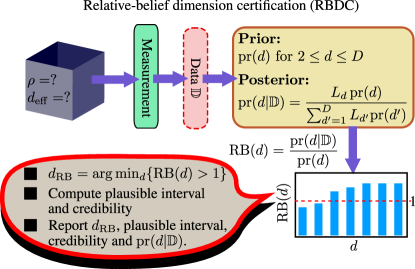
Figure 1: Schematic RBDC for general quantum tomography.

The procedure of RBDC, summarized in Fig. 1, is to take the smallest $d\equiv d_{\mathrm{RB}}$ that satisfies condition (1) as $d_{\mathrm{eff}}$. It is clear that neither additional assumption about $\varrho$ nor any other quantity is needed to carry out dimension certification with RB—everything is encoded in the dataset $\mathbb{D}$ waiting to be extracted. It is straightforward to see that for a $\mathbb{D}$ of very large sample-copy number $N$, the influence of each likelihood function $L_{d}$ overwhelms $\mathrm{pr}(d)$, so that in this data-dominant situation, $\mathrm{RB}(d)$ is essentially governed by $L_{d}$. As a larger Hilbert space surely contains the ML estimator derived from a smaller space, we have the monotonicity property $L_{d}\leq L_{d+1}$, and hence $\mathrm{RB}(d\geq d_{\mathrm{RB}})>1$ in the asymptotic limit. Evidently, the pathological prior that preferentially picks some $d=d_{0}$, that is the Kronecker-delta prior $\mathrm{pr}(d)=\delta_{d,d_{0}}$, ignores all data and must, of course, be excluded in any scientific inquiry. Under such a statistically natural and logical Bayesian system, where initial beliefs may be accepted or refuted solely by $\mathbb{D}$ without the need for ad hoc criteria, any quantum tomography procedure may be carried out through RBDC without spurious assumptions, including the insistence of $d_{\mathrm{eff}}$, using the same tomographic datasets that reconstruct $\varrho$.

Moreover, the posterior probability quantifies the strength of our belief that $d_{\mathrm{eff}}=d_{\mathrm{RB}}$ whenever $\mathrm{RB}(d_{\mathrm{RB}})>1$. If we think that this magnitude is too small, then we are free to choose another $d_{\mathrm{eff}}$ that gives a larger RB ratio, a feature that is fundamentally lacking in usual hypothesis testing [52].

The tools for assessing the credibility of $d_{\mathrm{RB}}$ are built into the Bayesian character of RBDC. In particular, we can assign a plausible interval $[d_{\mathrm{RB}},d_{\mathrm{RB}}+\Delta]$ for some integer $\Delta$ of credibility $C=\sum^{d_{\mathrm{RB}}+\Delta}_{d^{\prime}=d_{\mathrm{RB}}}\mathrm{pr}(d^{\prime}|\mathbb{D})\leq 1$, which is the conditional probability (given $\mathbb{D}$) that this interval contains all plausible $d$ such that $\mathrm{RB}(d)>1$. Since $L_{d}$ is monotonic in $d$, it is clear that all $d\geq d_{\mathrm{RB}}$ will be plausible for a large $N$. In this way, $d_{\mathrm{RB}}$ comes with natural error intervals endowed by the Bayesian RB framework. Operation-wise, $|L_{d}|$ can still be very small even for moderate values of $N$. Nonetheless, routine computation of all these elements is now possible with recent developments in storing ultra-high precision formats, ideal for coping with minuscule $L_{d}$ values [69]. Thus, RBDC reports the ML estimator, $d_{\mathrm{RB}}$ and its plausible interval, the corresponding $C$s and posterior probabilities.

There exist other well-known model-selection methods that minimize a class of information functions of the form $I_{\alpha,d}=\alpha\kappa_{d}-\log L_{d}$ with a positive $\alpha$ that scales sublinearly with $N$. Here, $\kappa_{d}$ is the number of degrees of freedom that is strictly-increasing in $d$. When applied to quantum-state tomography, $\kappa_{d}=d^{2}-1$. Special cases of this class includes Akaike’s ($\alpha=1$, AIC) and the Bayesian [$\alpha=(\log N)/2$, BIC] information criteria [67, 68]. From the monotonicity of $L_{d}$, it is clear that $I_{\alpha,d}$ is convex in $d$, where $d_{I}$ refers to the dimension that minimizes $I_{\alpha,d}$ whenever the minimum is stationary. On occasions where $I_{\alpha,d}$ exhibits a minimum plateau over $d$, $d_{I}$ is defined as the maximum dimension in this plateau region. Interestingly, we show in the Supplemental Material (SM) that in the large-$N$ limit, if $\mathrm{pr}(d)>0$, then RBDC typically announces a $d_{\mathrm{RB}}\geq d_{I}$ with very high probability, thereby rendering RBDC as a conservative quantum protocol for ascertaining the effective dimension of an unknown state.

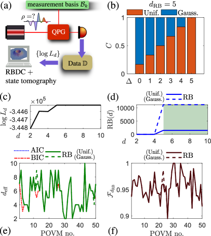
Figure 2: v(a) The experimental scheme for RBDC tomography on a degree-one temporal Hermite–Gaussian (HG₁) quantum state consists of measuring $K=11$ von Neumann bases $\{\mathcal{B}_{1},\mathcal{B}_{2}\ldots\mathcal{B}_{K}\}$ under random unitary rotations realized by the QPG, which form one IC POVM. The priors considered for RBDC are uniform [$\mathrm{pr}(d)=1/(D-1)$] and Gaussian [$\mathrm{pr}(d)\propto\exp(-(d-2)^{2})$], the latter of which reflects a stronger conviction that $d_{\mathrm{eff}}=2$ is sufficient to describe $\varrho$. We take $D=10$. (b) The credibilities $C$ for the plausible intervals $[d_{\mathrm{RB}},d_{\mathrm{RB}}+\Delta]$ with $0\leq\Delta\leq 2$ are plotted for one such POVM ($N\sim 10^{4}$ and $d_{\mathrm{RB}}=5$), where its corresponding (c) log-likelihood and (d) log-RB ratio follow the same trend over $d$ as $N$ is rather large [plausible interval of (b) shaded]. (e) Numerical evidence from 50 randomly generated POVMs verifies that the $d_{\mathrm{RB}}$s given by RBDC are never smaller than those of AIC and BIC even when log-likelihood monotonicity is absent. (f) The corresponding state-reconstruction fidelities $\mathcal{F}_{d_{\mathrm{RB}}}$ using RBDC are almost the same for both prior distributions for these large datasets.

RBDC in spectral-temporal state tomography.—A crucial application of RBDC is quantum tomography of all physical CV systems residing in an infinite-dimensional Hilbert space, but possessing a finite photon-number support. One promising platform that utilizes CV tomography is time-frequency encoding [70, 71, 72], which is employed in a plethora of quantum-information and communication tasks [73, 74, 75, 76, 77].

In the experiment, we generate states whose information is encoded on Hermite–Gaussian (HG) temporal modes, that is, field-orthogonal pulses with HG-shaped complex spectral amplitudes. We then execute a randomized compressive tomography on these states using a quantum pulse gate (QPG). The QPG is a dispersion-engineered sum-frequency generator in a periodically poled lithium niobate waveguide [78]. It combines a single-photon-level signal at telecom wavelengths and a strong classical pump pulse at around 860 nm. By shaping the complex amplitude of the pump pulse, the user defines the temporal mode that is selected by the QPG. The part of the signal that exhibits field overlap with this mode is upconverted and the converted output is detected with a single photon counter. A successful detection event implements a POVM onto the temporal mode defined by the pump [79]. Collecting counts for a set amount of time and for a set of IC pump temporal modes then allows for assessing the effective dimension of the state via RBDC.

Figure 2 showcases the positive performance of RBDC in determining the correct $d_{\mathrm{RB}}$ of a temporal HG state $\varrho=\ket{\mathrm{HG}_{n}}\bra{\mathrm{HG}_{n}}$ ($n=1$ for our experiments), with the temporal wave function $\langle t|\mathrm{HG}_{n}\rangle\propto\mathrm{e}^{\mbox{\footnotesize$-t^{2}/2$}}\mathrm{H}_{\,n}\!\left(t\right)$. All datasets obtained from the QPG possess persistent background noise caused by detector dark counts, leading to a very small bias towards diagonal matrix elements in $\widehat{\varrho}_{\textsc{ml}}(d)$ that do not vanish for any $d$. We remove this bias by directly incorporating the constraint that all nonzero diagonal elements of $\widehat{\varrho}_{\textsc{ml}}(d)$ are $>0.01$ directly into the ML reconstruction, in addition to the positivity constraint, by following modified projected gradients [80]. Such a noise subtraction may be viewed as additional prior information that enters the posterior computation for RBDC. After noise subtraction, using only evidence from datasets $\mathbb{D}$, RBDC with different prior beliefs consistently give effective dimensions that are larger than or equal to those of AIC and BIC, which are accompanied by easy-to-compute credibility $C$ for specified plausible intervals. In the SM, we present the original data with background noise, where all $d_{\mathrm{eff}}$s are typically large. These are tell-tale signatures of persistent systematic errors that need to be addressed, whereas BIC almost always gives overly optimistic conclusions that are unjustified by $\mathbb{D}$ through posterior probabilities.

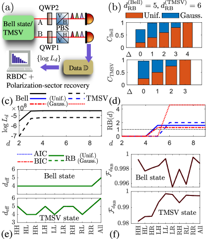
Figure 3: (a) The quantum polarimetry setup involves a source of either Bell or TMSV states respectively generated at $r=$1.96 dB and 2.12 dB. The QWP angles are set to correspond the two-arm polarization settings hh, hl, hr, lh, ll, lr, rh, rl and rr, where h, l and r are the standard horizontal, left- and right-circular polarizations. Here, $d_{\mathrm{eff}}$ or $d_{\mathrm{RB}}$ refers to the effective mode dimension in each arm. We have $D=9$ and the Gaussian prior $\propto\exp[-(d-5)^{2}]$. (b) Plots of $C$ for Bell- and TMSV-state plausible intervals for the combined datasets of all nine measurement settings are shown. (c,d) This time, $N\sim 10^{8}$ per setting, so that the overwhelming $\mathbb{D}$ has very low data noise and $L_{d}$ increases monotonically with $d$. (e,f) All model-selection methods coincide with such astronomical datasets, and in this figure, $\mathcal{F}_{d_{\mathrm{RB}}}=\sum^{d_{\mathrm{RB}}-1}_{m,n=0}\sqrt{p_{mn}\widehat{p}_{\mathrm{ML},mn}}$ is the Bhattacharyya fidelity between diagonal elements (or photon-number distributions) of the true state ($p_{mn}$) and ML estimator ($\widehat{p}_{\mathrm{ML},mn}$) extended to the $D$-dimensional Hilbert space. The RBDC performances with both priors are identical in such data-dominant situations.

RBDC in quantum polarimetry.—Apart from full quantum-state tomography, RBDC is also applicable for estimating key properties of a quantum source. One such scenario is quantum polarimetry for high-dimensional quantum systems to investigate polarization sectors [81], which encode interesting hidden quantum properties beyond the classical polarization description [82, 83, 84, 85, 86, 87, 88, 89, 90, 91, 92, 93, 94, 95, 96] and shall reveal the versatility of RBDC in certifying dimensions of DV systems. A typical polarimetry setup consists of wave plates and beam splitters that transform an incoming optical signal of unknown state $\varrho$. Coupled with, photon-number-resolving detectors of $\approx 90\%$ efficiency, these passive components realize POVMs that only probe the polarization sector of $\varrho$ that is smaller than the complete $d_{\mathrm{RB}}^{2}$-dimensional state space. Nevertheless, quantum polarimetry is an economical method to study the polarization sectors, which include photon-number statistics.

The polarimetry setup is operated by a dispersion-engineered periodically-poled potassium titanyl phosphate (PPKTP) waveguide inside a Sagnac interferometer [97, 98]. Type-II parametric down-conversion with significant multiphoton contributions is generated in the clockwise and counter-clockwise direction. A folded $4f$ spectrometer is used to select a narrow part of the pump-laser spectrum (100 fs pulse duration and 774 nm central wavelength), yielding pump pulses of 1 ps duration. Interfering the resulting spectrally-decorrelated signal and idler beams on the Sagnac polarizing beam splitter (PBS) generates either a Bell state [$\ket{\text{Bell}}\propto\sum^{\infty}_{m,n=0}\ket{m,n,n,m}(\tanh r)^{m+n}$] or a two-mode squeezed vacuum (TMSV) state [$\ket{\text{TMSV}}\propto\sum^{\infty}_{m,n=0}\ket{m,m,n,n}(\tanh r)^{m+n}$], where $r$ is the squeezing parameter, $\ket{m,n,m^{\prime},n^{\prime}}=\ket{m^{\prime}}_{\text{A},\textsc{h}}\ket{n^{\prime}}_{\text{A},\textsc{v}}\ket{m^{\prime}}_{\text{B},\textsc{h}}\ket{n^{\prime}}_{\text{B},\textsc{v}}$. The quarter-wave plates (QWP) on arms A and B each realizes $U_{\varphi}=\exp[-\mathrm{i}\varphi(a^{\dagger}_{\textsc{h}}a_{\textsc{h}}-a^{\dagger}_{\textsc{v}}a_{\textsc{v}})/2]$, and measuring only the h port on each arm (while tracing out the other v port) results in an overall POVM with only diagonal outcomes in the computational basis (see SM), implying that the probable elements are only the diagonal elements $p_{mn}\equiv\langle m,n|\varrho^{\prime}|m,n\rangle=(\mathrm{sech}\,r)^{4}\,(\tanh r)^{2(m+n)}$ of $\varrho^{\prime}=\mathrm{tr}_{\text{A},\textsc{v},\text{B},\textsc{v}}\{\ket{\text{Bell or TMSV}}\bra{\text{Bell or TMSV}}\}$.

Figure 3 shows the feasibility of carrying out RBDC for data $\mathbb{D}$ of very large copy numbers that are free of background noise. Note that the degree of freedom $\kappa_{d}=d-1$ for $I_{\alpha,d}$ since only the photon-number distribution of $\varrho$ is recoverable from this “traced-out” polarimetry scheme. In such data-dominant scenarios, the prior choice becomes irrelevant and RBDC is heavily influenced by $\mathbb{D}$. For such huge datasets that are also almost void of statistical or systematic errors, the fact that $L_{d}$ is so strongly peaked means that, almost always, $\mathrm{RB}(d)>1$ only when $L_{d_{\mathrm{RB}}}$ is the true maximum value $L_{d_{\mathrm{c}}}$ achieved by a $d$ greater than or equal to some critical dimension $d_{\mathrm{c}}\leq D$. In this case, $d_{\mathrm{RB}}=d_{\mathrm{c}}$ and convexity of $I_{\alpha,d}$ also implies that $d_{I}=d_{\mathrm{c}}$, so that $d_{I}=d_{\mathrm{RB}}$ (see SM), which is the reason why AIC, BIC and RBDC typically predict the same $d_{\mathrm{eff}}=d_{\mathrm{c}}$ in this astronomical sample limit.

The results are a testament to the possibility of computing posterior probabilities from such extremely small values of $L_{d}$ without running into numerical underflow problems. We owe this to modern ways of storing extremely tiny numbers, which permits routine usage of this highly reliable and logical Bayesian machinery for dimension certification on very general and realistic experimental data. All numerical values of $L_{d}$ and posterior probabilities used in Figs. 2(b) and 3(b) are tabulated in SM, with storage precision as high as $10^{-306872481}$.

Apart from the data-abundant examples presented in this work, RBDC works for any experimental scenario, including data-limited situations in which $N$ is small. In SM, we also present simulation data for such arbitrary situations.

Discussion.—We presented a completely assumptionless dimension-certification protocol that only analyzes the experimental dataset obtained to ascertain the smallest effective dimension that fully contains the given unknown quantum state for a chosen truncation basis. This scheme is based on the powerful method of relative belief that quantitatively assesses how well the dataset supports our belief that the state should be contained by a Hilbert space by comparing the posterior probability of this belief with the initial prior probability before the experiment was conducted.

We tested this protocol with real experimental data obtained from spectral-temporal and polarimetry measurements and demonstrated that relative-belief ratios and credibility computations are now a reality using modern numerical toolboxes that competently handle extremely small numbers without underflow issues. At the same time, we confirmed, with analytical arguments, that relative-belief dimension certification performs more conservatively than other specific kinds of information criteria. By trusting only the data and nothing else, our protocol never oversteps its boundaries and conclude a Hilbert space of an overly optimistic (smaller) dimension that is unjustified by the data. Thus, our work sets a concrete example of what a truly evidence-based prescription that is simple and feasible for any quantum experiment should be.

Note that RBDC, consequently, also does not assume a specific truncation basis used. If there is strong conviction that the unknown state is sparse under a privileged basis choice, then this basis may be used with this scheme to further reduce the obtained effective dimension. On the other hand, the protocol readily informs us when this conviction is wrong by yielding posterior probabilities smaller than the corresponding prior ones. Such a basis choice is but one of many types of prior knowledge one can incorporate in the Bayesian sense, yet the final verdict is never dependent on any ad hoc suppositions. This immediately motivates the goal of searching for the truncation basis that maximizes the relative-belief ratio in the quest for finding the truly smallest Hilbert space containing the unknown state.

Supplemental Material

Appendix A Conservative aspect of RBDC

Whether convexity in $I_{\alpha,d}$ is strict or not, as $d_{I}$ is the largest dimension for which $I_{\alpha,d}$ is minimized, the strict inequality,

$$\alpha\,\kappa_{d_{I}}-\log L_{d_{I}}<\alpha\kappa_{d_{I}+1}-\log L_{d_{I}+1}\,,$$ (2)

holds. However, we note that the case where $I_{\alpha,d}$ exhibits a minimum plateau requires $\log L_{d+1}=\log L_{d}+\alpha(\kappa_{d+1}-\kappa_{d})$ for some interval of $d$, which is almost improbable for arbitrary $N$ and $\mathbb{D}$.

If $L_{\mathrm{max}}=\max_{d}\{L_{d}\}$, then $\log L_{d_{I}}\leq\log L_{\mathrm{max}}$, which gives

$$\alpha\,\kappa_{d_{I}}-\log L_{\mathrm{max}}<\alpha\kappa_{d_{I}+1}-\log L_{d_{I}+1}\,,$$ (3)

or

$$\log L_{d_{I}+1}<\log L_{\mathrm{max}}+\alpha(\kappa_{d_{I}+1}-\kappa_{d_{I}})\,.$$ (4)

On the other hand, an $\mathrm{RB}(d=d_{\mathrm{RB}})>1$ implies that

$$\log L_{d_{\mathrm{RB}}}>\log\left(\sum^{D}_{d^{\prime}=2}L_{d^{\prime}}\mathrm{pr}(d^{\prime})\right)>\log(L_{d_{0}})+\log(\mathrm{pr}(d_{0}))\,,$$ (5)

where $d_{0}=\arg\max_{d}\{L_{d}\,\mathrm{pr}(d)\}$. To complete the argument, we first assume, for simplicity, a uniform $\mathrm{pr}(d)=1/(D-1)$, leading to

$$\log L_{d_{\mathrm{RB}}}>\log L_{\mathrm{max}}-\log(D-1)\,,$$ (6)

so that

$$\log L_{d_{I}}\leq\log L_{d_{I}+1}<\log L_{d_{\mathrm{RB}}}+\alpha(\kappa_{d_{I}+1}-\kappa_{d_{I}})+\log(D-1)\,.$$ (7)

Since $\alpha$ is sublinear in $N$ and all other terms are independent of $N$, we find that when (7) holds for $N\gg 1$, these terms are dominated by the log-likelihoods, which are of order $N$, such that $\log L_{d_{I}}<\log L_{d_{\mathrm{RB}}}$ with a very large probability. Finally, the nondecreasing property of the likelihood in $d$ tells us that $d_{I}<d_{\mathrm{RB}}$.

Note that for astronomical datasets ($N\rightarrow\infty$), the likelihood function $L_{d}$ peaks extremely sharply at some saturated maximum value $L_{d_{\mathrm{c}}}$ that is achieved for $d\geq d_{\mathrm{c}}$, where $d_{\mathrm{c}}$ is some critical dimension; that is, $\log L_{d}$ drops very quickly for $d<d_{\mathrm{c}}$. In this asymptotic case, we almost surely have $\log L_{d_{I}}=\log L_{d_{\mathrm{c}}}=\log L_{d_{\mathrm{RB}}}$. The existence of such a saturation may arise either when $\rho$ has a photon-number distribution that ends abruptly after certain photon number $d_{\mathrm{c}}-1$ (such as the situation for perfect Fock states and their superposition or mixtures, which is an idealized situation), or when the distribution tail becomes numerically indistinguishable from zero (that of a coherent state, or practically any physically-realizable quantum state for that matter). Then in this case, $d_{I}$ must be the smallest dimension for which $\log L_{d_{I}}=\log L_{d_{\mathrm{c}}}$, since $\alpha\kappa_{d_{I}}-\log L_{d_{\mathrm{c}}}<\alpha\kappa_{d_{I}+1}-\log L_{d_{\mathrm{c}}}$, which is obvious. On the other hand, by definition of RBDC, we also must have $d_{\mathrm{RB}}$ to be the smallest dimension for which $\log L_{d_{\mathrm{RB}}}=\log L_{d_{\mathrm{c}}}$, which concludes that $d_{\mathrm{I}}=d_{\mathrm{RB}}$ for such a situation.

For the case of arbitrary priors where $\mathrm{pr}(d)>0$ for any $d$, the easiest way out is to note that for $N\gg 1$, the variation of $L_{d}\,\mathrm{pr}(d)$ in $d$ is approximately that of $L_{d}$ [$\log L_{d}+\log\mathrm{pr}(d)\cong\log L_{d}$]. With this approximation, the above arguments follow.

Appendix B Maximum-likelihood estimators constrained with background-noise subtraction

The ML state estimators $\widehat{\varrho}_{\textsc{ml}}(d)$ are found using a highly efficient numerical procedure that maximizes the log-likelihood using projected-gradient methods [80]. Instead of walking the $A$ space through the parametrization $\rho=A^{\dagger}A/\mathrm{tr}\left\{A^{\dagger}A\right\}$, which results in search trajectories that hovers (zig-zags) around the global maximum, projected-gradient recipes suggest an iteration of two steps: an optimization update in the $\rho$-space followed by a projection of the unphysical result back to the state space. This projection is done by setting all negative eigenvalues to zero and a final trace renormalization.

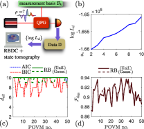
Figure 4: (a) The experimental scheme for RBDC tomography on the HG₁ temporal quantum state using the same 50 POVMs in Fig. 2 of the main text. All specifications are the same except that no background noise is subtracted. (b) All RB ratios are below 1 in this case. Thus, all dimensions are ruled out by the data due to lack of evidence. (c) This time, the $d_{\mathrm{eff}}$s are larger without background-noise subtraction. BIC is significantly more optimistic than all other methods. (d) The fidelities of the reconstructed states are, of course, generally lower now.

Additional simple constraints may be flexibly incorporated to augment the current projected-gradient procedure. In our context, we are interested in finding ML estimators that are also void of small diagonal-element biases (smaller than a particular threshold of, say, 0.01). After the state-space projection, we remove such biases by setting all diagonal elements of $\widehat{\varrho}_{\textsc{ml}}(d)$ that are smaller than this threshold value and their corresponding row and column elements to zero, followed by a trace renormalization. It is straightforward to see that positivity is still preserved, and so background-noise subtraction performed this way is therefore compatible with the above state-space projection. The resulting $\widehat{\varrho}_{\textsc{ml}}(d)$ shall therefore be physical and possess no diagonal-element bias.

We note that the imposition of this bias-free constraint would result in an ML problem that is nonconvex. In order to find the global maximum when $d=2$ (lowest dimension), we repeat the search multiple times to obtain a log-likelihood value that is heuristically close to the global maximum one. We do the same for $d>2$, but ensure that the maximal value should at least be equal (up to numerical precision, of course) to the previous lower dimension. If all ML estimators gave lower log-likelihood values, then we take the estimator for the previous dimension, pad it with zeros in the computational basis and consider this as the ML estimator for this dimension.

Appendix C Data with background noise (systematic errors)

It is clear that RBDC pays no attention to the type of datasets obtained in any experiment. It treats all datasets on the same footing and analyze them using the key elements found in Bayesian statistics: So long as the posterior distribution is larger than the prior for a particular dimension $d$, then the particular dataset is deemed to support the statement that a $d$-dimensional Hilbert space contains the unknown state $\rho$.

Figure 4 shows that if one applies RBDC on datasets containing background noise, then the effective dimension $d_{\mathrm{RB}}$ predicted by RBDC will generally be larger than AIC or BIC. With a (non-pathological) prior that reflects a stronger belief for a particular dimension, and if that dimension coincides with the true support dimension, then $d_{\mathrm{RB}}$ can be slightly smaller, partially subject to the verdict of the dataset according to the posterior probability. Even in this case, RBDC always consults the dataset, and only the dataset. No other spurious assumptions are made in such a dimension certification.

That $d_{\mathrm{RB}}$ is consistently large in this situation is not a drawback. Rather, it is a warning to the observer that the dataset holds systematic errors—overly optimistic model-selection procedures can lead to unjustified assertions than what the dataset dictates.

Appendix D Basics of quantum polarimetry

D.1 POVM for quantum polarimetry

To understand the fundamental principles, let us consider only a single arm comprising a PBS and two wave plates HWP ($\vartheta$) and QWP ($\varphi$). In the main text, this HWP is absent. At the end of the PBS, two photon-number-resolving detectors (PNRDs) are present to measure a certain number of photons at each port. The figure below shows a situation in which four single-photon pulses are measured at each port.

(8)

Here are the details of the POVM in point form:

1. Define the angular-momentum operators $J_{2}=\mathrm{i}(a_{\textsc{v}}^{\dagger}a_{\textsc{h}}-a_{\textsc{h}}^{\dagger}a_{\textsc{v}})/2$ and $J_{3}=(a_{\textsc{h}}^{\dagger}a_{\textsc{h}}-a_{\textsc{v}}^{\dagger}a_{\textsc{v}})/2$, where $a_{\textsc{h}}$ and $a_{\textsc{v}}$ are the polarization mode operators.

2. The unitary operator $U_{\vartheta,\varphi}=\mathrm{e}^{\mbox{\footnotesize$-\mathrm{i}\varphi J_{3}$}}\,\mathrm{e}^{\mbox{\footnotesize$-\mathrm{i}\vartheta J_{2}$}}$ represents the wave plate transformation [81].

3. For a given maximum number of photons $N_{0}$ impinging on each detector, we model the imperfect PNRD outcome of efficiency $\eta$ (set to be 0.9 in our context) as the normal-order form [98]

   $$\Pi^{(\eta)}_{n}=\binom{N}{n}\bm{:}\Pi^{n}(1-\Pi)^{N_{0}-n}\bm{:}\,,\,\,\text{where}~{}\Pi=1-\bm{:}\mathrm{e}^{\mbox{\footnotesize$-\eta a^{\dagger}a/N_{0}$}}\bm{:}\,.$$ (9)

   These outcomes generalize the on-off detector to arbitrary number of photons. As a demonstration, recall the identity $\bm{:}\mathrm{e}^{\mbox{\footnotesize$-\lambda a^{\dagger}a$}}\bm{:}\,\,=(1-\lambda)^{a^{\dagger}a}$ and consider the perfect situation of $\eta=1$. Then, $N_{0}=1$ gives rise to the familiar special case

   $$\Pi^{(\eta=1)}_{0}= \,\bm{:}\mathrm{e}^{\mbox{\footnotesize$-a^{\dagger}a$}}\bm{:}\,=0^{\,a^{\dagger}a}=\ket{\textsc{vac}}\bra{\textsc{vac}}\,,$$

   $$\Pi^{(\eta=1)}_{1}= \,1-\ket{\textsc{vac}}\bra{\textsc{vac}}=\ket{1}\bra{1}+\ket{2}\bra{2}+\ldots\,.$$ (10)

   When $N_{0}=2$, we have

   $$\Pi^{(\eta=1)}_{0}= \,\bm{:}\frac{1}{2^{2\,a^{\dagger}a}}\bm{:}\,\,=(1-2\log 2)^{a^{\dagger}a}\,,$$

   $$\Pi^{(\eta=1)}_{1}= \,2\bm{:}\left(1-\frac{1}{2^{a^{\dagger}a}}\right)\frac{1}{2^{a^{\dagger}a}}\bm{:}\,\,=2(1-\log 2)^{a^{\dagger}a}-2(1-2\log 2)^{a^{\dagger}a}\,,$$

   $$\Pi^{(\eta=1)}_{2}= \,\bm{:}\left(1-\frac{1}{2^{a^{\dagger}a}}\right)^{2}\bm{:}\,\,=\,\,\bm{:}\left(1-\frac{2}{2^{a^{\dagger}a}}+\frac{1}{2^{2a^{\dagger}a}}\right)\bm{:}\,\,=1-2(1-\log 2)^{a^{\dagger}a}+(1-2\log 2)^{a^{\dagger}a}\,.$$ (11)

4. The POVM elements representing the outcomes of (8) are therefore

   $$\Pi^{(\eta)}_{n_{1},n_{2}}(\vartheta,\varphi)=U_{\vartheta,\varphi}\Pi^{(\eta)}_{n_{1}}\otimes\Pi^{(\eta)}_{n_{2}}U_{\vartheta,\varphi}^{\dagger}\,.$$ (12)

We shall show that by truncating the Hilbert space for each port to $N_{0}$ photons, the number of linearly-independent POVM elements the set $\{\Pi^{(\eta)}_{n_{1},n_{2}}(\vartheta,\varphi)\}$ can generate is at most

$$D_{\mathrm{pol}}=2\sum^{N_{0}-1}_{k=0}(k+1)^{2}+(N_{0}+1)^{2}=\dfrac{1}{3}(N_{0}+1)(2N_{0}^{2}+4N_{0}+3)\,,$$ (13)

which is much smaller than the operator dimension $(N_{0}+1)^{4}$ of any two-mode state $\rho$ of Hilbert-space dimension $(N_{0}+1)^{2}$. Furthermore, if one port is traced over, then the number of linearly-independent single-port POVM elements is at most $N_{0}+1$.

D.2 Non-ICness of quantum polarimetry

Recall an important observation in [81] that any quantum polarimetry measurement can only probe the polarization sector of a quantum state $\rho$. To define this sector, we rewrite the two-mode Fock kets $\ket{n_{1},n_{2}}$ as a spin-$\frac{1}{2}$ angular-momentum eigenstate $\ket{S,m}$, where $S=(n_{1}+n_{2})/2$ and $m=(n_{1}-n_{2})/2$. Then, the polarization sector (or polarization state) $\rho_{\mathrm{pol}}$ is defined as

$$\rho_{\mathrm{pol}}=\bigoplus^{\infty}_{S=0}p(S)\rho^{(S)}=\sum^{\infty}_{S=0}p(S)\sum^{S}_{m=-S}\sum^{S}_{m^{\prime}=-S}\ket{S,m}\rho^{(S)}_{m,m^{\prime}}\bra{S,m^{\prime}}\,.$$ (14)

In other words, in the $\{\ket{S,m}\}$ basis, only constant-$S$ sectors $\rho^{(S)}$ of $\rho$ are probed by polarimetry POVMs.

D.2.1 Truncation of total photon number measured for the two ports

Suppose that $2N_{0}$ is the largest photon number for the two ports, that is $S=0,\frac{1}{2},1,\frac{3}{2},2,\ldots,\frac{2N_{0}}{2}$. Then the total number of free parameters characterizable by quantum polarimetry can be found by noting that $\rho^{(0)}_{m,m^{\prime}}$ is a single number, $\rho^{(1/2)}_{m,m^{\prime}}$ is two-dimensional and defined by $\ket{\frac{1}{2},-\frac{1}{2}}$ and $\ket{\frac{1}{2},\frac{1}{2}}$, $\rho^{(1)}_{m,m^{\prime}}$ is three-dimensional and spanned by $\ket{1,-1}$, $\ket{1,0}$ and $\ket{1,1}$, and so forth. So, this number is $D_{\mathrm{pol}}=1+2^{2}+3^{2}+\ldots+(2N_{0}+1)^{2}=\frac{1}{3}(N_{0}+1)(2N_{0}+1)(4N_{0}+3)$.

D.2.2 Truncation of total photon number measured for each port

If $N_{0}$ is now the largest photon number for each port, which is our experimental scenario, then the following counting scheme gives the correct $D_{\mathrm{pol}}$. Supposing that $N_{0}=1$, then the polarimetry POVM $\{\Pi^{(\eta)}_{n_{1},n_{2}}(\vartheta,\varphi)\}$ can probe sectors up to $S=1$. The relevant polarization sector from the maps

(15)

would then contain a one-dimensional vacuum sector, a two-dimensional one-photon Hermitian sector that gives 4 real parameters, and a one-dimensional two-photon sector. This tallies to $6$ free parameters. Notice that $\ket{0,2}$ and $\ket{2,0}$ are excluded since $N_{0}=1$ at each port. Thus, $D_{\mathrm{pol}}=1+4+1=6$ when $N_{0}=1$.

For $N_{0}=2$, the POVM can probe sectors up to $S=2$, so that

(16)

implies that $D_{\mathrm{pol}}=1+4+9+4+1=19$. From the above patterns, it easy to deduce Eq. (13).

Appendix E Measurement datasets for Figs. (2) and (3) of the main text and simulations for data-limited situations

For all experiments, von Neumann bases in the infinite-dimensional Hilbert space are measured. Each basis $\mathcal{B}_{k}$ comprises (in reality) a finite number of POVM elements $\Pi_{jk}$ such that $\sum_{j}\Pi_{jk}=1$ and corresponds to a detector-“click” probability column $\pmb{p}_{k}$ whose elements $p_{jk}=\mathrm{tr}\left\{\rho\Pi_{jk}\right\}$ sum to 1—$\sum_{j}p_{jk}=1$. The number of POVM elements would be associated with a maximal dimension $D$ for RBDC, the value of which is usually guided by physical intuition of the experiment, such as the average photon number, tail length of the photon-number distribution, et cetera. As each basis is measured independently with $N_{k}$ copies per basis, the total likelihood $L$ is just the product of the individual multinomial-type likelihoods. That is, for $K$ measured bases and a particular “click”-frequency sequence $\{n_{jk}\}$ such that $\sum_{j}n_{jk}=N_{k}$, $L=\prod^{K}_{k=1}L_{k}=\prod^{K}_{k=1}\prod_{j}p_{jk}^{n_{jk}}$.

We emphasize that the logic behind RBDC works for any experimental situation. The insistence that data must support one’s assertion by comparing the posterior and prior probabilities pays no attention to the kind of data that is being analyzed. In this section, we consider a CV source prepared in a Fock state of 7 photons. One arbitrarily-chosen von Neumann basis is measured, where we take $D=20$. The prior choices [uniform and Gaussian $\left(\propto\mathrm{e}^{\mbox{\footnotesize$-(d-8)^{2}$}}\right)$], log-likelihood graphs and RB ratios for four different $N$ values (one $\mathbb{D}$ each) are shown in (17) and (18). It is clear that when $N$ is this small, an informed prior can help guide the convergence of $d_{\mathrm{RB}}$ more efficiently as opposed to a completely ignorant one. The RBDC procedure formally supplies evidence supporting such an informed guess only if it is correct.

(17)

(18)

Appendix F Table of numerical values

Tables of likelihood values and posterior contents used to plot Figs. 2(b) and 3(b) in the main text. The decimal places showcase storage capabilities, not computational precision which is dictated by that of ML.

Table 1: Likelihood values and posterior probabilities ffrom the dataset of POVM no. 7 for Fig. 2(b) in the text.

Likelihood	$d$ $L_{d}$ 2 1.910200961849743785030610224731732032006327450641135205959787153e-149752 3 5.106857911370325091648503512521967863132578983385229925814312374e-149658 4 1.794717885295998128537139948794055184939542610517891728092474606e-149659 5 6.755446025787587091812436483073267911850465319370140060645363117e-149625 6 6.755446025787587091812436483073267911850465319370140060645363117e-149625 7 6.755446025787587091812436483073267911850465319370140060645363117e-149625 8 6.755446025787587091812436483073267911850465319370140060645363117e-149625 9 6.755446025787587091812436483073267911850465319370140060645363117e-149625 10 6.755446025787587091812436483073267911850465319370140060645363117e-149625
Uniform	$d$ $\mathrm{pr}(d|\mathbb{D})$ 2 4.712743255732553054521532547018926651753778872759252784183438783e-129 3 1.259936030839883114653205748522088712368481643488005315058207893e-34 4 4.427829730376093205762548271647074566243289026592105496299827386e-36 5 0.1666666666666666666666666666666666449297611976059325548194794794 6 0.1666666666666666666666666666666666449297611976059325548194794794 7 0.1666666666666666666666666666666666449297611976059325548194794794 8 0.1666666666666666666666666666666666449297611976059325548194794794 9 0.1666666666666666666666666666666666449297611976059325548194794794 10 0.1666666666666666666666666666666666449297611976059325548194794794
Gaussian	$d$ $\mathrm{pr}(d|\mathbb{D})$ 2 1.811492525702610273619644632523871842090688357968370020285770368e-123 3 1.781626975790019495910583089918198454779828033023700911111053681e-29 4 2.917819206131510044602153241393249605968452591884373208503656677e-32 5 0.9990888364735183604306543028149505613243627440237335371178507634 6 0.0009110510919670464577397712746462635210025962523776749399412791270 7 0.0000001124326367726086868358410450581788270436362962270528277584970265 8 0.000000000001877816258434481807624919489531665960511015092814392901090475765 9 4.244483309846593936193234147159523777178454647022659632446218542e-18 10 1.298397293813343080292908005916186515242034448853146959049695543e-24

Table 2: Likelihood values and posterior contents from different priors for the Bell-state combined dataset of all nine polarization settings used in Fig. 3(b) of the main text.

Likelihood	$d$ $L_{d}$ 2 8.403490385863592712990917327109636785426579254762189116001695376e-241771739 3 3.655739282866103174044744995755057155229460506918790692749954769e-198298861 4 6.330620382524476308070544809567671044319190406322579287081083635e-196822260 5 1.776792027639825604150877605451397800972526507582163108814115906e-196778830 6 1.776792027639825604150877605451397800972526507582163108814115906e-196778830 7 1.776792027639825604150877605451397800972526507582163108814115906e-196778830 8 1.776792027639825604150877605451397800972526507582163108814115906e-196778830 9 1.776792027639825604150877605451397800972526507582163108814115906e-196778830
Uniform	$d$ $\mathrm{pr}(d|\mathbb{D})$ 2 9.459171647709653534886755317970275165136876060380205043839921333e-44992910 3 4.114988390309414313454661644948699303165029949647399242731604008e-1520032 4 7.125899130618746242142348837497304737217532444365261039751559732e-43431 5 0.2 6 0.2 7 0.2 8 0.2 9 0.2
Gaussian	$d$ $\mathrm{pr}(d|\mathbb{D})$ 2 4.210267819553408908553507147335813649770725713580218068865734232e-44992913 3 2.718301595960439593842719321802808035882597596336721506037869889e-1520033 4 9.454795548003367249196222449106976134248370921079357367617165407e-43431 5 0.7213349069032195596568817076250338665875643824181071226498860823 6 0.2653642824490107955366354177322951490485674592347429120982628122 7 0.01321170967267805579371765694826247023434539773236961482957872417 8 0.00008901979954180955844229495404517222736201531945568018301054324833 9 0.00000008117554977945432292274036334190216074529532467023926183802934895

Table 3: Likelihood values and posterior contents from different priors for the TMSV-state combined dataset of all nine polarization settings used in Fig. 3(b) of the main text.

Likelihood	$d$ $L_{d}$ 2 1.222256227141671752091154406796389699070660098072229744455202464e-306872481 3 2.844096023090229079813918119779081530244493176898802665681025320e-230480082 4 8.480194198000157649647279087686896087251218208326448855277658249e-226267426 5 1.476921537445382768539500507106717819644837744873381994693482444e-226050278 6 4.145221565372174318775201702865502600615951978650069696694988681e-226006849 7 4.145221565372174318775201702865502600615951978650069696694988681e-226006849 8 4.145221565372174318775201702865502600615951978650069696694988681e-226006849 9 4.145221565372174318775201702865502600615951978650069696694988681e-226006849
Uniform	$d$ $\mathrm{pr}(d|\mathbb{D})$ 2 7.371477060189017748930867093088421250793582773000497335680827786e-80865634 3 1.715285888967237229526402291882300354038778693576490201836411362e-4473234 4 5.114439641080302793122772178037966165638469533725511505894716085e-260578 5 8.907373913273432802677936046871630921521915555456576299689449665e-43431 6 0.25 7 0.25 8 0.25 9 0.25
Gaussian	$d$ $\mathrm{pr}(d|\mathbb{D})$ 2 9.419298311571059005750921671935084393211215810269869590987778579e-80865637 3 3.252916814063418799244303185375878854919880381240512563418771974e-4473235 4 1.948130051599535872125222000144826411876368089914200843629733303e-260577 5 9.222826814913319689845696149798283514283166867987880881502717475e-43430 6 0.9522695487261826844081002875207288867423403130685955483059846066 7 0.04741070912706539274878167382556835549396161713625131659096852837 8 0.0003194508452872242773780641178805601027960203778077992646929174449 9 0.0000002913014646985657399745358221976609020494173453358383539476069818

References

- Plastino et al. [2015] A. Plastino, G. Bellomo, and A. R. Plastino, Quantum state space dimension as a quantum resource, Int. J. Quantum Inf. 13, 1550039 (2015).
- Brunner et al. [2008] N. Brunner, S. Pironio, A. Acin, N. Gisin, A. Méthot, and V. Scarani, Testing the dimension of Hilbert spaces, Phys. Rev. Lett. 100, 210503 (2008).
- Wehner et al. [2008] S. Wehner, M. Christandl, and A. C. Doherty, Lower bound on the dimension of a quantum system given measured data, Phys. Rev. A 78, 062112 (2008).
- Gallego et al. [2010] R. Gallego, N. Brunner, C. Hadley, and A. Acín, Device-independent tests of classical and quantum dimensions, Phys. Rev. Lett. 105, 230501 (2010).
- Hendrych et al. [2012] M. Hendrych, R. Gallego, M. Mičuda, N. Brunner, A. Acín, and J. P. Torres, Experimental estimation of the dimension of classical and quantum systems, Nat. Phys. 8, 588 (2012).
- Ahrens et al. [2012] J. Ahrens, P. Badziag, A. Cabello, and M. Bourennane, Experimental device-independent tests of classical and quantum dimensions, Nat. Phys. 8, 592 (2012).
- Dall’Arno et al. [2012] M. Dall’Arno, E. Passaro, R. Gallego, and A. Acín, Robustness of device-independent dimension witnesses, Phys. Rev. A 86, 042312 (2012).
- Brunner et al. [2013] N. Brunner, M. Navascués, and T. Vértesi, Dimension witnesses and quantum state discrimination, Phys. Rev. Lett. 110, 150501 (2013).
- Gühne et al. [2014] O. Gühne, C. Budroni, A. Cabello, M. Kleinmann, and J.-Å. Larsson, Bounding the quantum dimension with contextuality, Phys. Rev. A 89, 062107 (2014).
- Bowles et al. [2014] J. Bowles, M. T. Quintino, and N. Brunner, Certifying the dimension of classical and quantum systems in a prepare-and-measure scenario with independent devices, Phys. Rev. Lett. 112, 140407 (2014).
- D’Ambrosio et al. [2014] V. D’Ambrosio, F. Bisesto, F. Sciarrino, J. F. Barra, G. Lima, and A. Cabello, Device-independent certification of high-dimensional quantum systems, Phys. Rev. Lett. 112, 140503 (2014).
- Ahrens et al. [2014] J. Ahrens, P. Badziąg, M. Pawłowski, M. Żukowski, and M. Bourennane, Experimental tests of classical and quantum dimensionality, Phys. Rev. Lett. 112, 140401 (2014).
- Sun et al. [2016] Y.-N. Sun, Z.-D. Liu, J. Sun, G. Chen, X.-Y. Xu, Y.-C. Wu, J.-S. Tang, Y.-J. Han, C.-F. Li, and G.-C. Guo, Experimental realization of dimension witnesses based on quantum state discrimination, Phys. Rev. A 94, 052313 (2016).
- Cai et al. [2016] Y. Cai, J.-D. Bancal, J. Romero, and V. Scarani, A new device-independent dimension witness and its experimental implementation, J. Phys. A: Math. Theor. 49, 305301 (2016).
- Cong et al. [2017] W. Cong, Y. Cai, J.-D. Bancal, and V. Scarani, Witnessing irreducible dimension, Phys. Rev. Lett. 119, 080401 (2017).
- Sun et al. [2020] Y.-N. Sun, Z.-D. Liu, J. Bowles, G. Chen, X.-Y. Xu, J.-S. Tang, C.-F. Li, and G.-C. Guo, Experimental certification of quantum dimensions and irreducible high-dimensional quantum systems with independent devices, Optica 7, 1073 (2020).
- Sohbi et al. [2021] A. Sohbi, D. Markham, J. Kim, and M. T. Quintino, Certifying dimension of quantum systems by sequential projective measurements, Quantum 5, 472 (2021).
- Lanyon et al. [2009] B. P. Lanyon, M. Barbieri, M. P. Almeida, T. Jennewein, T. C. Ralph, K. J. Resch, G. J. Pryde, J. L. O’Brien, A. Gilchrist, and A. G. White, Simplifying quantum logic using higher-dimensional Hilbert spaces, Nat. Phys. 5, 134 (2009).
- Spekkens and Rudolph [2001] R. W. Spekkens and T. Rudolph, Degrees of concealment and bindingness in quantum bit commitment protocols, Phys. Rev. A 65, 012310 (2001).
- Massar [2002] S. Massar, Nonlocality, closing the detection loophole, and communication complexity, Phys. Rev. A 65, 032121 (2002).
- Molina-Terriza et al. [2005] G. Molina-Terriza, A. Vaziri, R. Ursin, and A. Zeilinger, Experimental quantum coin tossing, Phys. Rev. Lett. 94, 040501 (2005).
- Duclos-Cianci and Poulin [2013] G. Duclos-Cianci and D. Poulin, Kitaev’s -code threshold estimates, Phys. Rev. A 87, 062338 (2013).
- Campbell [2014] E. T. Campbell, Enhanced fault-tolerant quantum computing in -level systems, Phys. Rev. Lett. 113, 230501 (2014).
- Luo et al. [2019] Y.-H. Luo, H.-S. Zhong, M. Erhard, X.-L. Wang, L.-C. Peng, M. Krenn, X. Jiang, L. Li, N.-L. Liu, C.-Y. Lu, A. Zeilinger, and J.-W. Pan, Quantum teleportation in high dimensions, Phys. Rev. Lett. 123, 070505 (2019).
- Pawłowski and Brunner [2011] M. Pawłowski and N. Brunner, Semi-device-independent security of one-way quantum key distribution, Phys. Rev A 84, 010302 (2011).
- Woodhead and Pironio [2015] E. Woodhead and S. Pironio, Secrecy in prepare-and-measure Clauser-Horne-Shimony-Holt tests with a qubit bound, Phys. Rev. Lett. 115, 150501 (2015).
- Woodhead [2016] E. Woodhead, Semi device independence of the BB84 protocol, New J. Phys. 18, 055010 (2016).
- Goh et al. [2016] K. T. Goh, J.-D. Bancal, and V. Scarani, Measurement-device-independent quantification of entanglement for given hilbert space dimension, New J. Phys. 18, 045022 (2016).
- Primaatmaja et al. [2023] I. W. Primaatmaja, K. T. Goh, E. Y.-Z. Tan, J. T.-F. Khoo, S. Ghorai, and C. C.-W. Lim, Security of device-independent quantum key distribution protocols: a review, Quantum 7, 932 (2023).
- Lunghi et al. [2015] T. Lunghi, J. B. Brask, C. C. W. Lim, Q. Lavigne, J. Bowles, A. Martin, H. Zbinden, and N. Brunner, Self-testing quantum random number generator, Phys. Rev. Lett. 114, 150501 (2015).
- Miao et al. [2022] R.-H. Miao, Z.-D. Liu, Y.-N. Sun, C.-X. Ning, C.-F. Li, and G.-C. Guo, High-dimensional multi-input quantum random access codes and mutually unbiased bases, Phys. Rev. A 106, 042418 (2022).
- Mogilevtsev et al. [2017] D. Mogilevtsev, Y. S. Teo, J. Řeháček, Z. Hradil, J. Tiedau, R. Kruse, G. Harder, C. Silberhorn, and L. L. Sanchez-Soto, Extracting the physical sector of quantum states, New J. Phys. 19, 093008 (2017).
- Teo et al. [2016] Y. S. Teo, D. Mogilevtsev, A. Mikhalychev, J. Řeháček, and Z. Hradil, Crystallizing highly-likely subspaces that contain an unknown quantum state of light, Sci. Rep. 6, 38123 (2016).
- Banaszek [1999] K. Banaszek, Maximum-likelihood algorithm for quantum tomography, Acta Phys. Slov. 49, 633 (1999).
- Fiurášek [2001] J. Fiurášek, Maximum-likelihood estimation of quantum measurement, Phys. Rev. A 64, 024102 (2001).
- Paris and Řeháček [2004] M. G. A. Paris and J. Řeháček, eds., Quantum State Estimation, Lect. Not. Phys., Vol. 649 (Springer, Berlin, 2004).
- Řeháček et al. [2007] J. Řeháček, Z. Hradil, E. Knill, and A. I. Lvovsky, Diluted maximum-likelihood algorithm for quantum tomography, Phys. Rev. A 75, 042108 (2007).
- Teo et al. [2011] Y. S. Teo, H. Zhu, B.-G. Englert, J. Řeháček, and Z. Hradil, Quantum-state reconstruction by maximizing likelihood and entropy, Phys. Rev. Lett. 107, 020404 (2011).
- Teo [2015] Y. S. Teo, Introduction to Quantum-State Estimation (World Scientific, Singapore, 2015).
- Teo and Sánchez-Soto [2021] Y. S. Teo and L. L. Sánchez-Soto, Modern compressive tomography for quantum information science, Int. J. Quantum Inf. 19, 2140003 (2021).
- Teo et al. [2021] Y. S. Teo, S. Shin, H. Jeong, Y. Kim, Y.-H. Kim, G. I. Struchalin, E. V. Kovlakov, S. S. Straupe, S. P. Kulik, G. Leuchs, and L. L. Sánchez-Soto, Benchmarking quantum tomography completeness and fidelity with machine learning, New J. Phys. 23, 103021 (2021).
- Teo et al. [2020] Y. S. Teo, G. I. Struchalin, E. V. Kovlakov, D. Ahn, H. Jeong, S. S. Straupe, S. P. Kulik, G. Leuchs, and L. L. Sánchez-Soto, Objective compressive quantum process tomography, Phys. Rev. A 101, 022334 (2020).
- Kim et al. [2020] Y. Kim, Y. S. Teo, D. Ahn, D.-G. Im, Y.-W. Cho, G. Leuchs, L. L. Sánchez-Soto, H. Jeong, and Y.-H. Kim, Universal compressive characterization of quantum dynamics, Phys. Rev. Lett. 124, 210401 (2020).
- Gianani et al. [2020] I. Gianani, Y. Teo, V. Cimini, H. Jeong, G. Leuchs, M. Barbieri, and L. Sánchez-Soto, Compressively certifying quantum measurements, PRX Quantum 1, 020307 (2020).
- Ahn et al. [2019a] D. Ahn, Y. S. Teo, H. Jeong, F. Bouchard, F. Hufnagel, E. Karimi, D. Koutný, J. Řeháček, Z. Hradil, G. Leuchs, and L. L. Sánchez-Soto, Adaptive compressive tomography with no a priori information, Phys. Rev. Lett. 122, 100404 (2019a).
- Ahn et al. [2019b] D. Ahn, Y. S. Teo, H. Jeong, D. Koutný, J. Řeháček, Z. Hradil, G. Leuchs, and L. L. Sánchez-Soto, Adaptive compressive tomography: A numerical study, Phys. Rev. A 100, 012346 (2019b).
- Gross et al. [2010] D. Gross, Y.-K. Liu, S. T. Flammia, S. Becker, and J. Eisert, Quantum state tomography via compressed sensing, Phys. Rev. Lett. 105, 150401 (2010).
- Kalev et al. [2015] A. Kalev, R. L. Kosut, and I. H. Deutsch, Quantum tomography protocols with positivity are compressed sensing protocols, npj Quantum Inf. 1, 15018 (2015).
- Goyeneche et al. [2015] D. Goyeneche, G. Cañas, S. Etcheverry, E. S. Gómez, G. B. Xavier, G. Lima, and A. Delgado, Five measurement bases determine pure quantum states on any dimension, Phys. Rev. Lett. 115, 090401 (2015).
- Baldwin et al. [2016] C. H. Baldwin, I. H. Deutsch, and A. Kalev, Strictly-complete measurements for bounded-rank quantum-state tomography, Phys. Rev. A 93, 052105 (2016).
- Steffens et al. [2017] A. Steffens, C. A. Riofrío, W. McCutcheon, I. Roth, B. A. Bell, A. McMillan, M. S. Tame, J. G. Rarity, and J. Eisert, Experimentally exploring compressed sensing quantum tomography, Quantum Sci. Technol. 2, 025005 (2017).
- Evans [2015] M. Evans, Measuring Statistical Evidence Using Relative Belief (Chapman & Hall, New York, 2015).
- Evans [2016] M. Evans, Measuring statistical evidence using relative belief, Comput. Struct. Biotechnol. J. 14, 91 (2016).
- Evans and Tomal [2018] M. Evans and J. Tomal, Measuring statistical evidence and multiple testing, FACETS 3, 563 (2018).
- Al-Labadi et al. [2018] L. Al-Labadi, Z. Baskurt, and M. Evans, Statistical reasoning: Choosing and checking the ingredients, inferences based on a measure of statistical evidence with some applications, Entropy 20, 289 (2018).
- Nott et al. [2020] D. J. Nott, X. Wang, M. Evans, and B.-G. Englert, Checking for prior-data conflict using prior-to-posterior divergences, Stat. Sci. 35, 234 (2020).
- Nott et al. [2021] D. J. Nott, M. Seah, L. Al-Labadi, M. Evans, H. K. Ng, and B.-G. Englert, Using prior expansions for prior-data conflict checking, Bayesian Anal. 16, 203 (2021).
- Englert et al. [2021] B.-G. Englert, M. Evans, G. H. Jang, H. K. Ng, D. Nott, and Y.-L. Seah, Checking for model failure and for prior-data conflict with the constrained multinomial model, Metrika 84, 1141 (2021).
- Evans and Frangakis [2023] M. Evans and C. Frangakis, On resolving problems with conditionality and its implications for characterizing statistical evidence, Sankhya Ser. A 85, 1103 (2023).
- Shang et al. [2013] J. Shang, H. K. Ng, A. Sehrawat, X. Li, and B.-G. Englert, Optimal error regions for quantum state estimation, New J. Phys. 15, 123026 (2013).
- Li et al. [2016] X. Li, J. Shang, H. K. Ng, and B.-G. Englert, Optimal error intervals for properties of the quantum state, Phys. Rev. A 94, 062112 (2016).
- Teo et al. [2018] Y. S. Teo, C. Oh, and H. Jeong, Bayesian error regions in quantum estimation I: analytical reasonings, New J. Phys. 20, 093009 (2018).
- Oh et al. [2018] C. Oh, Y. S. Teo, and H. Jeong, Bayesian error regions in quantum estimation II: analytical reasonings, New J. Phys. 20, 093010 (2018).
- Oh et al. [2019a] C. Oh, Y. S. Teo, and H. Jeong, Efficient bayesian credible-region certification for quantum-state tomography, Phys. Rev. A 100, 012345 (2019a).
- Oh et al. [2019b] C. Oh, Y. S. Teo, and H. Jeong, Probing Bayesian credible regions intrinsically: A feasible error certification for physical systems, Phys. Rev. Lett. 123, 040602 (2019b).
- Sim et al. [2019] J. Y. Sim, J. Shang, H. K. Ng, and B.-G. Englert, Proper error bars for self-calibrating quantum tomography, Phys. Rev. A 100, 022333 (2019).
- Burnham and Anderson [2002] K. Burnham and D. Anderson, Model Selection and Multi-Model Inference: A Practical Information-Theoretic Approach (Springer-Verlag, New York, 2002).
- Stoica and Selen [2004] P. Stoica and Y. Selen, Model-order selection: a review of information criterion rules, IEEE Signal Process. Mag. 21, 36 (2004).
- D’Errico [2018] J. D’Errico, HPF - a big decimal class (2018), https://www.mathworks.com/matlabcentral/fileexchange/36534-hpf-a-big-decimal-class .
- Brecht et al. [2015] B. Brecht, D. V. Reddy, C. Silberhorn, and M. G. Raymer, Photon temporal modes: A complete framework for quantum information science, Phys. Rev. X 5, 041017 (2015).
- Slussarenko and Pryde [2019] S. Slussarenko and G. J. Pryde, Photonic quantum information processing: A concise review, Appl. Phys. Rev. 6, 041303 (2019).
- Gil-Lopez et al. [2021] J. Gil-Lopez, Y. S. Teo, S. De, B. Brecht, H. Jeong, C. Silberhorn, and L. L. Sánchez-Soto, Universal compressive tomography in the time-frequency domain, Optica 8, 1296 (2021).
- Zhou et al. [2003] D. L. Zhou, B. Zeng, Z. Xu, and C. P. Sun, Quantum computation based on d-level cluster state, Phys. Rev. A 68, 062303 (2003).
- Eckstein et al. [2011] A. Eckstein, B. Brecht, and C. Silberhorn, A quantum pulse gate based on spectrally engineered sum frequency generation, Opt. Express 19, 13770 (2011).
- Babazadeh et al. [2017] A. Babazadeh, M. Erhard, F. Wang, M. Malik, R. Nouroozi, M. Krenn, and A. Zeilinger, High-dimensional single-photon quantum gates: Concepts and experiments, Phys. Rev. Lett. 119, 180510 (2017).
- Cozzolino et al. [2019] D. Cozzolino, B. Da Lio, D. Bacco, and L. K. Oxenløwe, High-dimensional quantum communication: Benefits, progress, and future challenges, Adv. Quantum Technol. 2, 1900038 (2019).
- Raymer and Walmsley [2020] M. G. Raymer and I. A. Walmsley, Temporal modes in quantum optics: then and now, Physica Scripta 95, 064002 (2020).
- Brecht et al. [2014] B. Brecht, A. Eckstein, R. Ricken, V. Quiring, H. Suche, L. Sansoni, and C. Silberhorn, Demonstration of coherent time-frequency Schmidt mode selection using dispersion-engineered frequency conversion, Phys. Rev. A 90, 030302 (2014).
- Ansari et al. [2017] V. Ansari, G. Harder, M. Allgaier, B. Brecht, and C. Silberhorn, Temporal-mode measurement tomography of a quantum pulse gate, Phys. Rev. A 96, 063817 (2017).
- Shang et al. [2017] J. Shang, Z. Zhang, and H. K. Ng, Superfast maximum-likelihood reconstruction for quantum tomography, Phys. Rev. A 95, 062336 (2017).
- Goldberg et al. [2021] A. Z. Goldberg, P. d. l. Hoz, G. Björk, A. B. Klimov, M. Grassl, G. Leuchs, and L. L. Sánchez-Soto, Quantum concepts in optical polarization, Adv. Opt. Photon. 13, 1 (2021).
- Klyshko [1992] D. N. Klyshko, Multiphoton interference and polarization effects, Phys. Lett. A 163, 349 (1992).
- Klyshko [1997] D. M. Klyshko, Polarization of light: Fourth-order effects and polarization-squeezed states, JETP 84, 1065 (1997).
- Tsegaye et al. [2000] T. Tsegaye, J. Söderholm, M. Atatüre, A. Trifonov, G. Björk, A. V. Sergienko, B. E. A. Saleh, and M. C. Teich, Experimental Demonstration of Three Mutually Orthogonal Polarization States of Entangled Photons, Phys. Rev. Lett. 85, 5013 (2000).
- Usachev et al. [2001] P. Usachev, J. Söderholm, G. Björk, and A. Trifonov, Experimental verification of differences between classical and quantum polarization properties, Opt. Commun. 193, 161 (2001).
- Luis [2002] A. Luis, Degree of polarization in quantum optics, Phys. Rev. A 66, 013806 (2002).
- Agarwal and Chaturvedi [2003] G. S. Agarwal and S. Chaturvedi, Scheme to measure quantum Stokes parameters and their fluctuations and correlations, J. Mod. Opt. 50, 711 (2003).
- Sánchez-Soto et al. [2007] L. L. Sánchez-Soto, E. C. Yustas, G. Björk, and A. B. Klimov, Maximally polarized states for quantum light fields, Phys. Rev. A 76, 043820 (2007).
- Björk et al. [2010] G. Björk, J. Söderholm, L. L. Sánchez-Soto, A. B. Klimov, I. Ghiu, P. Marian, and T. A. Marian, Quantum degrees of polarization, Opt. Commun. 283, 4440 (2010).
- Sánchez-Soto et al. [2013] L. L. Sánchez-Soto, A. B. Klimov, P. de la Hoz, and G. Leuchs, Quantum versus classical polarization states: when multipoles count, J. Phys. B: At. Mol. Opt. Phys. 46, 104011 (2013).
- Björk et al. [2015] G. Björk, M. Grassl, P. de la Hoz, G. Leuchs, and L. L. Sánchez-Soto, Stars of the quantum universe: extremal constellations on the Poincaré sphere, Physica Scripta 90, 108008 (2015).
- Björk et al. [2015] G. Björk, A. B. Klimov, P. de la Hoz, M. Grassl, G. Leuchs, and L. L. Sánchez-Soto, Extremal quantum states and their Majorana constellations, Phys. Rev. A 92, 031801 (2015).
- Shabbir and Björk [2016] S. Shabbir and G. Björk, SU(2) uncertainty limits, Phys. Rev. A 93, 052101 (2016).
- Goldberg and James [2017] A. Z. Goldberg and D. F. V. James, Perfect polarization for arbitrary light beams, Phys. Rev. A 96, 053859 (2017).
- Bouchard et al. [2017] F. Bouchard, P. de la Hoz, G. Björk, R. W. Boyd, M. Grassl, Z. Hradil, E. Karimi, A. B. Klimov, G. Leuchs, J. Řeháček, and L. L. Sánchez-Soto, Quantum metrology at the limit with extremal Majorana constellations, Optica 4, 1429 (2017).
- Goldberg [2020] A. Z. Goldberg, Quantum theory of polarimetry: From quantum operations to Mueller matrices, Phys. Rev. Res. 2, 023038 (2020).
- Meyer-Scott et al. [2018] E. Meyer-Scott, N. Prasannan, C. Eigner, V. Quiring, J. M. Donohue, S. Barkhofen, and C. Silberhorn, High-performance source of spectrally pure, polarization entangled photon pairs based on hybrid integrated-bulk optics, Opt. Express 26, 32475 (2018).
- Prasannan et al. [2022] N. Prasannan, J. Sperling, B. Brecht, and C. Silberhorn, Direct measurement of higher-order nonlinear polarization squeezing 10.48550/arxiv.2204.07083 (2022).