Current progress on the semileptonic form factors for $\bar{B}\to D^{\ast}\ell\bar{\nu}$ decay using the Oktay-Kronfeld action

Abstract

We present recent progress in calculating the semileptonic form factors $h_{A_{1}}(w)$ for the $\bar{B}\to D^{\ast}\ell\bar{\nu}$ decays. We use the Oktay-Kronfeld (OK) action for the charm and bottom valence quarks and the HISQ action for light quarks. We adopt the Newton method combined with the scanning method to find a good initial guess for the $\chi^{2}$ minimizer in the fitting of the 2pt correlation functions. The main advantage is that the Newton method lets us to consume all the time slices allowed by the physical positivity. We report the first, reliable, but preliminary results for $h_{A_{1}}(w)/\rho_{A_{1}}$ at zero recoil ($w=1$). Here we use a MILC HISQ ensemble ($a=0.12$ fm, $M_{\pi}$ = 220 MeV, and $N_{f}=2+1+1$ flavors).

1 Introduction

We present update of data analysis on the 2pt and 3pt correlation functions to obtain the semileptonic form factors for the $\bar{B}\to D^{\ast}\ell\bar{\nu}$ decays. We adopt the Newton method combined with the scanning method [1] to find a good initial guess for the $\chi^{2}$ minimizer in the fitting of the 2pt correlation functions. We find that the multiple time slice combinations help to distinguish the global minimum of $\chi^{2}$ and its local minima reliably. The Newton method leads to a self-consistent fit which consumes all the time slices allowed by the physical positivity [2, 3]. The results of data analysis on the 2pt correlation functions are used as inputs to the fitting of the 3pt correlation functions. As a result, we report the first, reliable, but preliminary results for $h_{A_{1}}(w)/\rho_{A_{1}}$ at zero recoil ($w=1$), obtained using the MILC HISQ ensemble in Table 1.

$a$ (fm)	$N_{f}$	$N_{s}^{3}\times N_{t}$	$M_{\pi}$ (MeV)	$am_{l}$	$am_{s}$	$am_{c}$
0.1184(10)	$2+1+1$	$32^{3}\times 64$	216.9(2)	0.00507	0.0507	0.628

Table 1: Details on the MILC HISQ ensemble used for the numerical study [4].

2 Flow chart of the data analysis

The 2-point (2pt) correlation function is defined as [5],

$$C(t) =\sum_{\alpha=1}^{4}\sum_{\bf{x}}\left\langle\mathcal{O}^{\dagger}_{\alpha}(t,{\bf x})\mathcal{O}_{\alpha}(0)\right\rangle\,,\qquad$$ (1)

where an interpolating operator for heavy-light mesons $\mathcal{O}_{\alpha}(t,{\bf x})$ is

$$\mathcal{O}_{\alpha}(t,{\bf x}) =\left[\bar{\psi}(t,{\bf x})\,\Gamma\,\Omega(t,{\bf x})\right]_{\alpha}\chi(t,{\bf x})\,,\qquad\Omega(t,{\bf x})\equiv\gamma_{1}^{\;x_{1}}\gamma_{2}^{\;x_{2}}\gamma_{3}^{\;x_{3}}\gamma_{4}^{\;t}\,.$$ (2)

Here, $\Gamma=\gamma_{5}$ ($\Gamma=\gamma_{j}$) for the pseudoscalar (vector) meson. Here, $\psi$ is a heavy quark field in the OK action [6], $\chi$ is a light quark field in the HISQ staggered action [7], and the subscript $\alpha$ represents taste degrees of freedom for staggered quarks.

We measure meson propagators (i.e. 2pt correlators in Eq. (1)) on the lattice. In the lattice QCD, the lattice Hilbert space consists of states of quarks and gluons, but the physical Hilbert space consists of states of hadrons. Hence, in order to extract physical information on hadronic states from the 2pt correlator, we use the spectral decomposition in the physical Hilbert space to obtain the fitting functional form $f(t)$. The fitting function of the $m+n$ fit is

$$f(t) =g(t)+g(T-t)\,,$$

$$g(t) =A_{0}\,e^{-E_{0}\,t}\left[1+R_{2}\,e^{-\Delta E_{2}\,t}\left(1+R_{4}\,e^{-\Delta E_{4}\,t}\left(\cdots\left(1+R_{2m-2}\,e^{-\Delta E_{2m-2}\,t}\right)\cdots\right)\right)\right.$$

$$\hphantom{=}\left.-(-1)^{t}\,R_{1}\,e^{-\Delta E_{1}\,t}\left(1+R_{3}\,e^{-\Delta E_{3}\,t}\left(\cdots\left(1+R_{2n-1}\,e^{-\Delta E_{2n-1}\,t}\right)\cdots\right)\right)\right]$$ (3)

where $\Delta E_{i}\equiv E_{i}-E_{i-2}$, $E_{-1}\equiv E_{0}$ , $R_{i}\equiv\dfrac{A_{i}}{A_{i-2}}$ and $A_{-1}\equiv A_{0}$. The subscript ₀ represents the ground state in the physical Hilbert space. Hence, $A_{0}$ and $E_{0}$ represents the amplitude and energy of the ground state. In the $m+n$ fit, $m$ ($n$) is the number of even (odd) time-parity states, which are kept in the fitting, while higher excited states in each time-parity channel are truncated.

Symbol	Description	Example
$\bar{\lambda}\pm\sigma(\lambda)$	average and error of a fit parameter $\lambda$	$\bar{A}_{0}\pm\sigma(A_{0}),\ldots$
$\lambda_{p}\pm\sigma_{p}(\lambda)$	prior information on a fit parameter $\lambda$	$[A_{0}]_{p}\pm\sigma_{p}(A_{0}),\ldots$
$\sigma_{p}^{\text{mf}}(\lambda)$	$\sigma_{p}(\lambda)$ obtained by the maximal fluctuation of data	$\sigma_{p}^{\text{mf}}(A_{0}),\ldots$
$\sigma_{p}^{\text{sc}}(\lambda)$	$\sigma_{p}(\lambda)$ obtained by the signal cut ($\sigma_{p}^{\text{sc}}(\lambda)=|\bar{\lambda}_{p}|$)	$\sigma_{p}^{\text{sc}}(A_{0}),\ldots$
$\sigma_{p}^{\max}(\lambda)$	$\min\bigl{(}\;\sigma_{p}^{\text{mf}}(\lambda),\;\sigma_{p}^{\text{sc}}(\lambda)\bigr{)}$	$\sigma_{p}^{\max}(A_{0}),\ldots$
$\sigma_{p}^{\text{opt}}(\lambda)$	optimal prior width of $\lambda$ in Eq. (5)	$\sigma_{p}^{\text{opt}}(A_{0}),\ldots$
$\sigma_{\sigma}(\lambda)$	error of error for $\lambda$, that is, error of $\sigma(\lambda)$	$\sigma(A_{0})\pm\sigma_{\sigma}(A_{0}),\ldots$

(a) Notation and convention

Symbol	Description
$\sigma(A_{0};\max)$	$\sigma(A_{0})$ when we set $\sigma_{p}(A_{0})=\sigma_{p}^{\max}(A_{0})$ and $\sigma_{p}(E_{0})=\sigma_{p}^{\max}(E_{0})\}$
$\sigma(E_{0};\max)$	$\sigma(E_{0})$ when we set $\sigma_{p}(A_{0})=\sigma_{p}^{\max}(A_{0})$ and $\sigma_{p}(E_{0})=\sigma_{p}^{\max}(E_{0})\}$

(b) Notation used for stability tests

Table 2: Notation and convention used in this article.

Our notation and convention is described in Table 2.

To determine fit parameters, $A_{0}$, $E_{0}$, $\{R_{j}$, $\Delta E_{j}\}$, we use sequential Bayesian method. We obtain fit parameters which minimizes the $\chi^{2}$. Using the fit function given in Eq. (3), we adopt the Broyden-Fletcher-Goldfarb-Shanno (BFGS) algorithm [8, 9, 10, 11] for the $\chi^{2}$ minimizer, which belongs to the quasi-Newton method. The quasi-Newton method needs an initial guess for the fit parameters. Here, we denote the initial guess as $A_{0}^{g}$, $E_{0}^{g}$, $\{R_{j}^{g}$, $\Delta E_{j}^{g}\}$. The superscript ^g represents the “initial guess”. A good initial guess reduces the number of iterations in the BFGS minimizer, which saves the computing cost dramatically [1]. In order to find a good initial guess directly from the data, we use the multi-dimensional Newton method [12, 13] combined with the scanning method [1]. We present the flow chart for the sequential Bayesian method in the following to describe the logistics.

1. Do the 1st fit.  [e.g.] Do 1+0 fit with 2 parameters: {$A_{0}$, $E_{0}$}

2. Feed the previous fit results as prior information for the next fit: $\lambda_{p}=\bar{\lambda}\,,\;\sigma_{p}(\lambda)=\sigma_{p}^{\max}(\lambda)$. We do not impose any constraint on new fit parameters which are not included in the previous fit. [e.g.] Results for the 1+0 fit are used as prior information on the 1+1 fit such that $[A_{0}]_{p}=\bar{A}_{0}$, $\sigma_{p}(A_{0})=\sigma_{p}^{\max}(A_{0})=\sigma_{p}^{\text{sc}}(A_{0})$ and $[E_{0}]_{p}=\bar{E}_{0}$, $\sigma_{p}(E_{0})=\sigma_{p}^{\max}(E_{0})=\sigma_{p}^{\text{mf}}(E_{0})$ with no constraint on $R_{1}$ and $\Delta E_{1}$.

   In order to give a general picture of our methodology, let us consider the $m+n$ fit, in which we want to determine $N=2(m+n)$ fit parameters. Hence, we should select $N$ time slices such as $\{t_{1},t_{2},\ldots,t_{N}\}$, to determine the initial guess $A_{0}^{g}$, $E_{0}^{g}$, $\{R_{j}^{g}$, $\Delta E_{j}^{g}\}$ by solving the following equations using the Newton method.

   $$q(t_{j}) \equiv\frac{f(t_{j})-C(t_{j})}{C(t_{j})}=0\,,\quad\text{with}\quad j=1,\cdots,N$$ (4)

   where $C(t)$ is data for the 2pt correlation functions in Eq. (1) and $f(t)$ is the fit function in Eq. (3).

   1. We find all the possible combinations of $N$ time slices which satisfy the following conditions.

      • We choose $N$ time slices within the fit range: $t_{\min}\leq t\leq t_{\max}$.

      • $t_{\min}$ should be included.

      • The number of even time slices should be equal to that of odd time slices in order to avoid a bias.

   2. Use the Newton method for each time slice combination to obtain a good initial guess for the $\chi^{2}$ minimizer:

      1. Take $i$-th time slice combination ($1\leq i\leq N_{c}$, $N_{c}$ is the total number of the time slice combinations).

      2. Recycle fit results from the previous fit ($[m-1]+n$ fit or $m+[n-1]$ fit) to set part of the initial guess for the Newton method.

      3. Use the scanning method [1] to set the remaining part of the initial guess for the Newton method.

      4. Run the Newton method.

      5. If the Newton method finds roots, then save them. If it fails, discard the $i$-th time slice combination. [e.g.] The failure rate is about $\approx 21\%$ for the 1+1 fit.

      6. Take the next $\bigl{(}$i.e. ($i+1$)-th$\bigr{)}$ time slice combination, and repeat the loop (Step-2(Step-2B)Step-2B1–Step-2(Step-2B)Step-2B6) until we consume all the time slice combinations.

   3. Perform the least $\chi^{2}$ fitting with the initial guess obtained by the Newton method.

   4. Sort results for $\chi^{2}$, check the $\chi^{2}$ distribution, and find out whether the $\chi^{2}$ minimizer converges to the global minimum or a local minimum.

3. Perform stability tests to obtain optimal prior widths. [e.g.] Determine {$\sigma_{p}^{\text{opt}}(A_{0})$, $\sigma_{p}^{\text{opt}}(E_{0})$}.

4. Save the current fitting results ([e.g.] 1+1 fit) into the 1st fitting.

5. Take the next fitting ([e.g.] 2+1 fit) as the current fitting.

6. Go back to Step-2 and repeat the loop until we consume all the time slices allowed by the physical positivity [2, 3]. [e.g.] 1+0 fit $\to$ 1+1 fit $\to$ 2+1 fit $\to$ 2+2 fit $\to$ $\cdots$.

The stability test condition for the sequential Bayesian method is

1. We have freedom to adjust $\lambda_{p}$ so that $|\bar{\lambda}-\lambda_{p}|\ll\sigma_{\sigma}(\lambda)$. One way to achieve this criterion is $|\bar{\lambda}-\lambda_{p}|<10^{-4}\sigma(\lambda)\ll\sigma_{\sigma}(\lambda)$ . Here the scaling factor $10^{-4}$ is obtained empirically for our statistical sample of $\approx 1000$ gauge configurations.

2. $\sigma_{p}(\lambda)$ should not disturb $\sigma(\lambda)$ such that $|\sigma(\lambda,\sigma_{p}(\lambda))-\sigma(\lambda,\max)|\ll\sigma_{\sigma}(\lambda)$ .

3. Based on condition (i) and (ii), we find the optimal prior width $\sigma^{\text{opt}}_{p}$. Here, $\sigma^{\text{opt}}_{p}$ is the minimum value of the prior width which does not disturb $\sigma(\lambda)$ of the fitting results such that

   $$\sigma_{p}^{\text{opt}}=\min(\sigma_{p})\ \text{for}\ \forall\sigma_{p}\in\{\sigma_{p}|\bar{\lambda}(\sigma_{p})\circeq\lim_{\sigma_{p}^{t}\to\infty}\bar{\lambda}(\sigma_{p}^{t}),\ \sigma(\lambda,\sigma_{p})\circeq\lim_{\sigma_{p}^{t}\to\infty}\sigma(\lambda,\sigma_{p}^{t})\}$$ (5)

Here the new equal symbol ($\circeq$) means that they are equal within the statistical uncertainty of $\sigma_{\sigma}(\lambda)$.

Let us explain the stability test (Step-3), using the $2+1$ fit as an example. In Fig. 1, we describe how to set the optimal prior widths $\sigma_{p}^{\text{opt}}(A_{0})$ and $\sigma_{p}^{\text{opt}}(E_{0})$ in the $2+1$ fit. In the case of $\sigma(A_{0})$ in Fig. 1 (1(a)), we plot $\sigma(A_{0})$ as a function of $\sigma_{p}(A_{0})$ in the unit of $\sigma(A_{0};\max)$ while we fix $\sigma_{p}(E_{0})$ to its maximum value: $\sigma_{p}(E_{0})=\sigma_{p}^{\max}(E_{0})=\sigma_{p}^{\text{mf}}(E_{0})$. Here we find that $\sigma_{p}^{\text{opt}}(A_{0})=20\times[\sigma(A_{0};\max)]$, which corresponds to the red (dashed) lines and red cross symbol in Fig. 1 (1(a)). Here the blue cross symbol and green (dashed) lines represents $\sigma(A_{0};\max)$ and the blue dotted lines represents the error of error $\sigma_{\sigma}(A_{0})$ of $\sigma(A_{0};\max)$.

In Fig. 1 (1(b)), we present the same kind of a plot for $\sigma(E_{0})$ with the same color convention as Fig. 1 (1(a)). Here we find that $\sigma_{p}^{\text{opt}}(E_{0})=25\times[\sigma(E_{0};\max)]$.

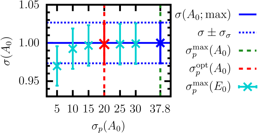
(a) $\sigma_{p}^{\text{opt}}(A_{0})$ in the unit of $\sigma(A_{0};\max)$.

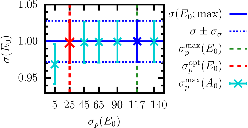
(b) $\sigma_{p}^{\text{opt}}(E_{0})$ in the unit of $\sigma(E_{0};\max)$.

Figure 1: Results of the stability tests to find optimal prior widths for the 2+1 fit.

3 Application of the Newton method to the 2+2 fit

3.1 Example for Step-2Step-2A

As explained in Ref. [1], we use the multi-dimensional Newton method [12, 13] to obtain a good initial guess for the $\chi^{2}$ minimizer in the $m+n$ correlator fit. For the $2+2$ fit, we should determine 8 fit parameters: $A_{0}$, $E_{0}$, $\{R_{j}$, $\Delta E_{j}\}$ with $j=1,2,3$. Hence, we need an initial guess: $A_{0}^{g}$, $E_{0}^{g}$, $\{R_{j}^{g}$, $\Delta E_{j}^{g}\}$ ($j=1,2,3$).

In order to find an initial guess, we need 8 time slices ($T_{8}$) so that we can use the Newton method to find roots:

$$q(t_{k}) \equiv\frac{f(t_{k})-C(t_{k})}{C(t_{k})}=0\,,\quad k=1,2,\ldots,8$$ (6)

where $t_{k}\in T_{8}$, $f(t)$ is the fitting function, and $C(t)$ is the 2pt correlator data. The 8 time slices in $T_{8}$ should be chosen within the fit range $t_{\min}\leq t\leq t_{\max}$ with $t_{\min}=3$ and $t_{\max}=30$. It is required to set $t_{1}$ to $t_{1}=t_{\min}$. The number of even (odd) time slices is 14 (13) except for $t_{1}=t_{\min}$. Hence, the total number of the possible combinations for $T_{8}$ is 286,286.

$${}_{14}C_{4}\times{}_{13}C_{3} =\text{286,286}$$ (7)

3.2 Description of Step-2Step-2B

In Step-2Step-2B, we run the Newton method. For example, in 2+2 fit, we select a time slice combination out of the 286,286 combinations [Step-2(Step-2B)Step-2B1]. We need another initial guess as input to run the Newton method: $A_{0}^{gn}$, $E_{0}^{gn}$, $\{R_{j}^{gn}$, $\Delta E_{j}^{gn}\}$ where the superscript ^gn indicates the initial guess for the Newton method. We use fit results from the 2+1 fit to set up $A_{0}^{gn}$, $E_{0}^{gn}$, $\{R_{j}^{gn}$, $\Delta E_{j}^{gn}\}$ ($j=1,2$) [Step-2(Step-2B)Step-2B2]. We use the scanning method in Ref. [1] to determine $R_{3}^{gn}$ and $\Delta E_{3}^{gn}$ [Step-2(Step-2B)Step-2B3].

Now, we run the Newton method to find roots: $A_{0}^{g}$, $E_{0}^{g}$, $\{R_{j}^{g}$, $\Delta E_{j}^{g}\}$ [Step-2(Step-2B)Step-2B4]. If the Newton method finds a root, save them. Otherwise, discard it [Step-2(Step-2B)Step-2B5]. It turns out that the Newton method can find 16,574 roots out of the 286,286 combinations, while the rest fails. We select 1,242 roots randomly out of the whole 16,574 roots in order to monitor statistics for the $\chi^{2}$ distribution.

3.3 Description of Step-2Step-2C and Step-2Step-2D

For each root that the Newton method can find successfully, we use it as an input to perform the least $\chi^{2}$ fitting [Step-2Step-2C]. For each root, we determine the statistics for $A_{0}$, $E_{0}$, $\{R_{j}$, $\Delta E_{j}\}$ ($j=1,2,3$) and $\chi^{2}$/d.o.f, using the jackknife resampling. Using the 1,242 roots, we check whether the $\chi^{2}$ minimizer reaches the global minimum or local minima.

ID	$N_{r}$	$\chi^{2}$/d.o.f.	note
2+2/G	1000	0.4091(82)	global minimum
2+2/L1	167	0.6093(88)	$\Delta E_{3}<0$
2+2/L2	54	3.766(26)	$R_{3}<O(10^{-9})\approx 0$ or $R_{3}<0$

Table 3: Patterns of the $\chi^{2}$ distribution. Here, $N_{r}$ means the number of roots obtained by the Newton method. Here G represents the global minimum and L represents the local minima.

We summarize patterns for the $\chi^{2}$ distribution in the Table 3. Among 1,242 roots, 1,000 roots converges to the global minimum (pattern ID = 2+2/G). We find two local minima of $\chi^{2}$: the pattern ID = 2+2/L1 (167 roots) and the pattern ID = 2+2/L2 (54 roots). The 2+2/L1 pattern gives consistent results of $\Delta E_{3}=-0.409(55)<0$, which is definitely unphysical and wrong. The 2+2/L2 pattern gives consistent results of $R_{3}<O(10^{-9})\approx 0$ or $R_{3}<0$, which are unphysical and wrong. There are 21 values of the $\chi^{2}$/d.o.f. between the 2+2/L1 and 2+2/L2 patterns, which also gives wrong results for $R_{3}$ or $\Delta E_{3}$. Table 3 shows that we can find the global minimum of the $\chi^{2}$ distribution with the Newton method reliably. In addition, we find that the local minima of the $\chi^{2}$ distribution always come up with unphysical (= wrong) results for $R_{3}$ or $\Delta E_{3}$.

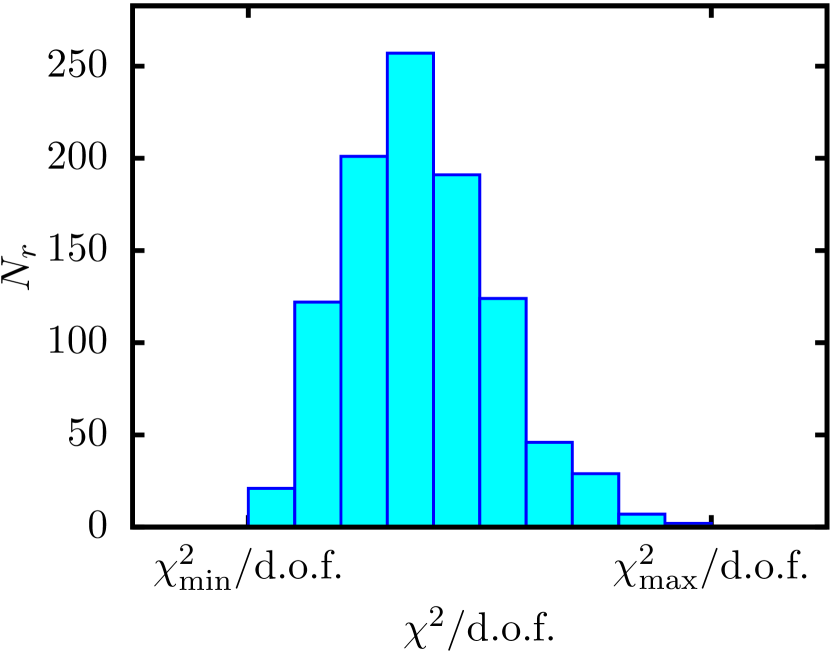
(a) Histogram of the $\chi^{2}_{d}$ distribution. We use the same notation as in Table 3. Here $\chi^{2}_{d}\equiv\chi^{2}/\text{d.o.f.}$, $\chi^{2}_{\min}\equiv\min(\chi^{2})$, and $\chi^{2}_{\max}\equiv\max(\chi^{2})$.

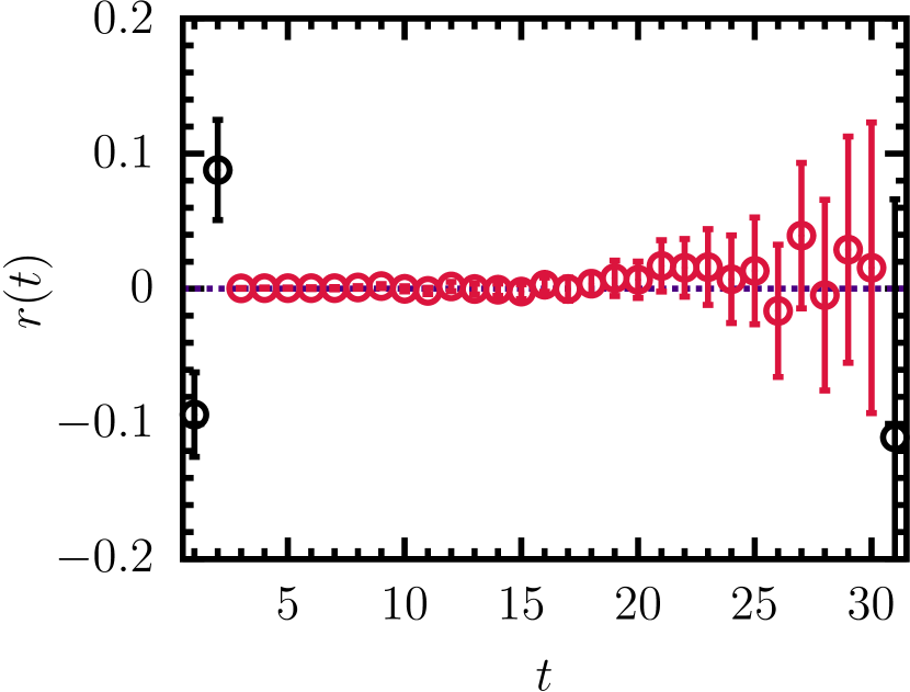
(b) Residual $r(t)=\dfrac{f(t)-C(t)}{|C(t)|}$. Here the red color represents the fit range ($3\leq t\leq 30$). The errors are purely statistical.

Figure 2: $\chi^{2}$ distribution and residual coming from the data analysis on the $B$-meson propagators.

In Fig. 2 (2(a)), we show the histogram of the $\chi^{2}$/d.o.f. distribution of the 2+2/G pattern. This indicates that the $\chi^{2}$ minimizer find the global minimum with about $\approx 80\%$ probability which indicates that once out of five times the $\chi^{2}$ minimizer converges to local minima. Hence, this is a clear advantage of using the Newton method to find a good initial guess for the $\chi^{2}$ minimizer. Out of the set of multiple roots of the Newton method, a subset find the global minimum for the $\chi^{2}$ distribution, and another subset reach the local minima, which we can discard without loss of generality.

In Fig. 2 (2(a)), $\Delta\chi^{2}/\text{d.o.f.}=\chi^{2}_{\max}/\text{d.o.f.}-\chi^{2}_{\min}/\text{d.o.f.}\cong 10^{-8}$ is significantly less than the statistical error ($\cong 0.0082$) of the $\chi^{2}/\text{d.o.f.}$. This indicates that the $\chi^{2}$ distribution has sharp peak.

The residual plot of $B$ meson 2pt correlator for the $2+2$ fit is given in Fig. 2 (2(b)). Note that we consumed up all the possible time slices allowed by the physical positivity [2, 3].

4 Preliminary result on $h_{A_{1}}(w=1)/\rho_{A_{1}}$: $B\to D^{\ast}\ell\nu$ form factor at zero recoil

The semileptonic form factor $h_{A_{1}}(w)$ at zero recoil (i.e. $w=1$) can be obtained with the Hashimoto ratio [14]:

$$h_{A_{1}}(w=1) =\rho_{A_{1}}\sqrt{\frac{\langle D^{\ast}_{0}|A^{cb}_{j}|{B}_{0}\rangle_{\text{L}}\,\langle{B}_{0}|A^{bc}_{j}|D^{\ast}_{0}\rangle_{\text{L}}}{\langle D^{\ast}_{0}|V^{cc}_{4}|D^{\ast}_{0}\rangle_{\text{L}}\,\langle{B}_{0}|V^{bb}_{4}|{B}_{0}\rangle_{\text{L}}}}\,,\qquad\rho_{A_{1}}=\sqrt{\frac{Z_{A}^{cb}\,Z_{A}^{bc}}{Z_{V}^{cc}\,Z_{V}^{bb}}}\,.$$ (8)

The one-loop matching calculation of $\rho_{A_{1}}$ is underway [15]. Here we present preliminary results on blind (i.e. $\rho_{A_{1}}=1$) $h_{A_{1}}(w=1)$ in this work. The subscript ₀ in Eq. (8) represents the ground states at zero momentum ($\vec{p}_{X}=0$ with $X=B,\ D^{\ast}$). We want to extract the four ground state matrix elements: $\langle D^{\ast}_{0}|A^{cb}_{j}|{B}_{0}\rangle_{\text{L}}$, $\langle{B}_{0}|A^{bc}_{j}|D^{\ast}_{0}\rangle_{\text{L}}$, $\langle D^{\ast}_{0}|V^{cc}_{4}|D^{\ast}_{0}\rangle_{\text{L}}$, and $\langle{B}_{0}|V^{bb}_{4}|{B}_{0}\rangle_{\text{L}}$ from the 3pt correlation functions. The 3pt correlation functions are calculated on the lattice and so the Hilbert space consists in quark and gluon states. The Hilbert space for physical observables such as the matrix elements consists in hadronic states. For example, when we fit the 2pt correlation functions for $B$-meson propagators, we obtain results for $A_{0}$, $E_{0}$ (i.e. information on the $B_{0}$ ground state), $R_{1}$, $\Delta E_{1}$ (i.e. the $B_{1}$ excited state with odd time-parity), $R_{2}$, $\Delta E_{2}$ (i.e. the $B_{2}$ excited state with even time-parity) and so on. We can obtain similar results for $D^{\ast}$-meson propagators. The fitting functional form for the 3pt correlation functions calculated on the lattice in the $B\to D^{\ast}$ channel is

$$f_{T_{\text{sep}}}^{B\to D^{\ast}}\left(t\right) =\left\langle D_{0}^{\ast}\right|A_{j}^{cb}\left|B_{0}\right\rangle_{\text{L}}\,k_{0}^{D^{\ast}}\left(t\right)k_{0}^{B}\left(T_{\text{sep}}-t\right)+\left\langle D_{0}^{\ast}\right|A_{j}^{cb}\left|B_{2}\right\rangle_{\text{L}}\,k_{0}^{D^{\ast}}\left(t\right)k_{2}^{B}\left(T_{\text{sep}}-t\right)$$

$$\hphantom{=\ }+\left\langle D_{1}^{\ast}\right|A_{j}^{cb}\left|B_{1}\right\rangle_{\text{L}}\,k_{1}^{D^{\ast}}\left(t\right)k_{1}^{B}\left(T_{\text{sep}}-t\right)+\left\langle D_{2}^{\ast}\right|A_{j}^{cb}\left|B_{0}\right\rangle_{\text{L}}\,k_{2}^{D^{\ast}}\left(t\right)k_{0}^{B}\left(T_{\text{sep}}-t\right)$$

$$\hphantom{=\ }+\left\langle D_{1}^{\ast}\right|A_{j}^{cb}\left|B_{3}\right\rangle_{\text{L}}\,k_{1}^{D^{\ast}}\left(t\right)k_{3}^{B}\left(T_{\text{sep}}-t\right)+\left\langle D_{2}^{\ast}\right|A_{j}^{cb}\left|B_{2}\right\rangle_{\text{L}}\,k_{2}^{D^{\ast}}\left(t\right)k_{2}^{B}\left(T_{\text{sep}}-t\right)$$

$$\hphantom{=\ }+\left\langle D_{3}^{\ast}\right|A_{j}^{cb}\left|B_{1}\right\rangle_{\text{L}}\,k_{3}^{D^{\ast}}\left(t\right)k_{1}^{B}\left(T_{\text{sep}}-t\right)+\left\langle D_{3}^{\ast}\right|A_{j}^{cb}\left|B_{3}\right\rangle_{\text{L}}\,k_{3}^{D^{\ast}}\left(t\right)k_{3}^{B}\left(T_{\text{sep}}-t\right)\,,$$ (9)

$$k_{0}^{X}\left(t\right) =\sqrt{A_{0}^{X}}\,e^{-E_{0}^{X}\,t}\,,\qquad\qquad\quad k_{1}^{X}\left(t\right)=\sqrt{A_{0}^{X}R_{1}^{X}}\,e^{-\left(E_{0}^{X}+\Delta E_{1}^{X}\right)\,t}\left(-1\right)^{t+1}\,,$$

$$k_{2}^{X}\left(t\right) =\sqrt{A_{0}^{X}R_{2}^{X}}\,e^{-\left(E_{0}^{X}+\Delta E_{2}^{X}\right)\,t}\,,\quad k_{3}^{X}\left(t\right)=\sqrt{A_{0}^{X}R_{1}^{X}R_{3}^{X}}\,e^{-\left(E_{0}^{X}+\Delta E_{1}^{X}+\Delta E_{3}^{X}\right)\,t}\left(-1\right)^{t+1}\,.$$ (10)

The $k_{j}^{X}(t)$ ($j=0,1,2,3$, $X=B,D^{\ast}$) comes from the fit results for the 2pt correlation functions for the $B$ and $D^{\ast}$ mesons. Hence, we determine the lattice matrix elements simply by a linear fit. As a result, we obtain $\langle D^{\ast}_{0}|A^{cb}_{j}|{B}_{0}\rangle_{\text{L}}$. We can apply the same kind of fitting to the $D^{\ast}\to B$, $B\to B$, and $D^{\ast}\to D^{\ast}$ channels. As a results, we obtain the rest of the lattice matrix elements: $\langle{B}_{0}|A^{bc}_{j}|D^{\ast}_{0}\rangle_{\text{L}}$, $\langle D^{\ast}_{0}|V^{cc}_{4}|D^{\ast}_{0}\rangle_{\text{L}}$, $\langle{B}_{0}|V^{bb}_{4}|{B}_{0}\rangle_{\text{L}}$.

In Fig. 3 we present results for $h_{A_{1}}(w=1)/\rho_{A_{1}}$. Here the green circles represent our results for $h_{A_{1}}(w=1)/\rho_{A_{1}}$ with no contamination from exited states, while the red squares represent those obtained using the $\bar{R}$ ratio [16] which include some contamination from excited states by construction. The black cross represents the FNAL-MILC result for $h_{A_{1}}(w=1)/\rho_{A_{1}}$ which is obtained using the $\bar{R}$ ratio with the Fermilab action for bottom and charm quarks, and the asqtad action for light quarks with $N_{f}=2+1$ [16].

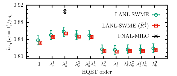
Figure 3: $h_{A_{1}}(w=1)/\rho_{A_{1}}$ in the order of the HQET power counting. Here $\lambda_{c}\cong 1/5$, and $\lambda_{b}\cong 1/17$.

When we do the linear fit over the 3pt correlation functions, we could not use the full covariance fitting but the diagonal approximation [17] due to unwanted bias by strong correlation between different time slices. We find that off-diagonal elements of the correlation matrix $\rho(t_{i},t_{j})$ with $t_{i}\neq t_{j}$ are close to one. This issue needs further investigation.

References

- [1] T. Bhattacharya et al. PoS LATTICE2021 (2021) 136 [2204.05848].
- [2] M. Luscher Commun. Math. Phys. 54 (1977) 283.
- [3] M. Luscher and P. Weisz Nucl. Phys. B 240 (1984) 349.
- [4] A. Bazavov et al. Phys. Rev. D87 (2013) 054505 [1212.4768].
- [5] A. Bazavov et al. Phys. Rev. D85 (2012) 114506 [1112.3051].
- [6] M.B. Oktay and A.S. Kronfeld Phys. Rev. D78 (2008) 014504 [0803.0523].
- [7] E. Follana et al. Phys. Rev. D75 (2007) 054502 [hep-lat/0610092].
- [8] C.G. Broyden IMA Journal of Applied Mathematics 6 (1970) 76.
- [9] R. Fletcher The Computer Journal 13 (1970) 317.
- [10] D. Goldfarb Mathematics of Computation 24 (1970) 23.
- [11] D.F. Shanno Mathematics of Computation 24 (1970) 647.
- [12] W.H. Press et al., Numerical Recipes, Cambridge University Press, 3 ed. (2007), pp 477–483.
- [13] C.G. Broyden Mathematics of Computation 19 (1965) 577.
- [14] S. Hashimoto et al. Phys. Rev. D 61 (1999) 014502 [hep-ph/9906376].
- [15] J.A. Bailey and S. Lee, in preparation.
- [16] Fermilab Lattice and MILC collaboration Phys. Rev. D 89 (2014) 114504 [1403.0635].
- [17] B. Yoon et al. J. Korean Phys. Soc. 63 (2013) 145 [1101.2248].