Kernel-U-Net: Symmetric and Hierarchical Architecture for Multivariate Time Series Forecasting

Abstract

Time series forecasting task predicts future trends based on historical information. Transformer-based U-Net architectures, despite their success in medical image segmentation, have limitations in both expressiveness and computation efficiency in time series forecasting as evidenced in YFormer. To tackle these challenges, we introduce Kernel-U-Net, a symmetric and hierarchical U-shape neural network architecture. The kernel-U-Net encoder compresses gradually input series into latent vectors, and its symmetric decoder subsequently expands these vectors into output series. Specifically, Kernel-U-Net separates the procedure of partitioning input time series into patches from kernel manipulation, thereby providing the convenience of executing customized kernels. Our method offers two primary advantages: 1) Flexibility in kernel customization to adapt to specific datasets; 2) Enhanced computational efficiency, with the complexity of the Transformer layer reduced to linear. Experiments on seven real-world datasets, considering both multivariate and univariate settings, demonstrate that Kernel-U-Net’s performance either exceeds or meets that of the existing state-of-the-art model PatchTST in the majority of cases and outperforms Yformer. The source code for Kernel-U-Net will be made publicly available for further research and application.

1 Introduction

Time series forecasting predicts future trends based on recent historical information. It allows experts to track the incoming situation and react timely in critical cases. Its applications range from different domains such as predicting the road occupancy rates from different sensors in the city Lai et al. (2018), monitoring influenza-like illness weekly patient cases Wu et al. (2021), monitoring electricity transformer temperature in the electric power long-term deployment Zhou et al. (2021) or forecasting temperature, pressure and humidity in weather station Liu et al. (2022b) etc.

Over the past few decades, time series forecasting solutions have evolved from traditional statistical methodsKhandelwal et al. (2015) and machine learning techniquesPersson et al. (2017) to deep learning-based solutions, such as recurrent neural networks(RNN) Tokgöz and Ünal (2018), Long Short-term Memory (LSTM) Kong et al. (2017), Temporal Convolutional Network (TCN) Hewage et al. (2020) and Transformer-based model Li et al. (2019).

Among the Transformer models applying to time series data, Informer Zhou et al. (2021), Autoformer Wu et al. (2021), and FEDformer Zhou et al. (2022) are the best variants that incrementally improved the quality of prediction. As a recent paper Zeng et al. (2023) challenges the efficiency of Transformer-based models with a simple linear layer model NLinear, the authors in Nie et al. (2023) argued that the degrades of performance comes from the wrong application of transformer modules on a point-wise sequence and the ignorance of patches. By adding a linear patch layer, their model PatchTST successfully relieved the overfitting problem of transformer modules and reached state-of-the-art results.

We observe that models display distinct strengths depending on the dataset type. For instance, NLinear stands out for its efficiency in handling univariate time series tasks, particularly with small-size datasets. On the other hand, PatchTST is noteworthy for its expressiveness in multivariate time series tasks on large-size datasets. These contrasting attributes highlight the necessity for a unified but flexible architecture. This architecture would aim to integrate various modules easily, allowing for specific customized solutions. Such integration should not only ensure a balance between computational efficiency and expressiveness but also respond to requests for rapid development and testing.

The Convolutional U-net, as a classic and highly expressive model in medical image segmentationRonneberger et al. (2015), features a symmetric encoder and decoder structure that is elegant in its design. This model’s structure is particularly suited to the time series forecasting task, as both inputs and outputs in this context are typically derived from the same distribution. The first U-shape model adapted for time series forecasting was the YformerMadhusudhanan et al. (2023), which incorporated Transformers in both its encoder and decoder components. As mentioned previously, employing Transformers on point-wise data has the potential to cause overfitting issues. Therefore, our investigation aims to discover if there is a U-shape architecture effective in time series forecasting, which also possesses the capability to integrate various modules flexibly, thus facilitating the specific customization of solutions.

To tackle this problem, we propose a symmetric and hierarchical architecture, Kernel-U-Net (K-U-Net), inspired by convolutional U-net and Yformer for time series forecasting. K-U-Net provides convenience for composing particular models with custom kernels that follow the design pattern. By replacing linear kernels with transformer or LSTM kernels, the model gains enhanced expressiveness, allowing it to capture more complex patterns and dependencies in the data. Furthermore, the hierarchical structure of K-U-Net exponentially reduces the input length at each level, thereby concurrently decreasing the complexity involved in learning such sequences. Notably, when Transformer modules are utilized in the second or higher-level layers, the computation cost remains linear, ensuring efficiency in processing.

To fully study the performance and efficiency of K-U-Net, we conduct experiments for time series forecasting tasks on several widely used benchmark datasets. We compose 30 variants of K-U-Net by placing different kernels at different layers and then we choose the best candidates for fine-tuning. Our results show that in time series forecasting, K-U-Net exceeds or meets the state-of-the-art results, such as NLinearZeng et al. (2023) and PatchTST, in the majority of cases.

In summary, the contributions of this work include:

• We propose Kernel-U-Net, a symmetric and hierarchical architecture that partitions input sequences into small patches at each layer of the network.

• Kernel-U-Net generalizes the concept of kernels and provides convenience for composing particular models with custom kernels that follow the design pattern.

• The computation complexity is guaranteed in linear when employing Transformer kernels at the second or higher layers.

• Kernel-U-Net exceeds or meets the state-of-the-art results in most cases.

We conclude that Kernel-U-Net stands out as a highly promising option for large-scale time series forecasting tasks. Its symmetric and hierarchical design provides a balance of low computational complexity and high expressiveness. In most scenarios, it either surpasses or is slightly below the state-of-the-art results. Furthermore, its adaptability in fast-paced development and testing environments is ensured by the use of flexible, customizable kernels.

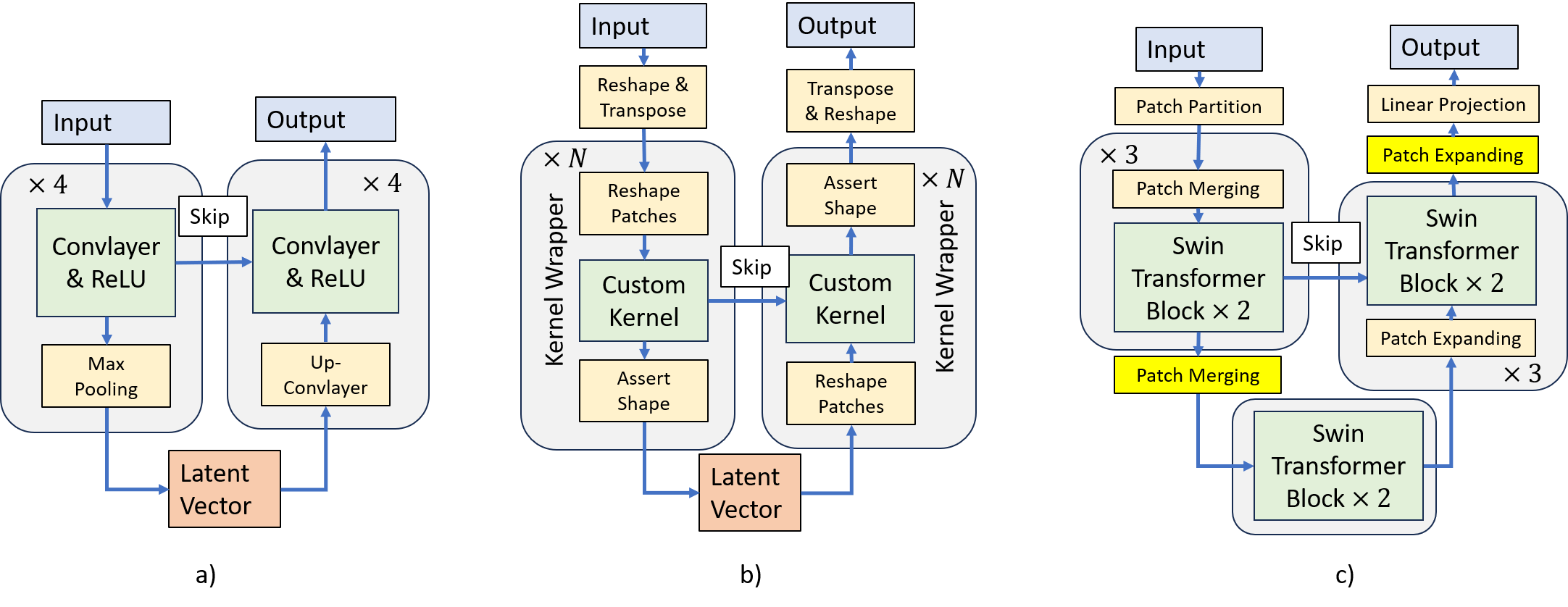
Figure 1: Comparison of the structures of different U-Net. a) classic Convolutional U-Net, b) Kernel U-Net, c) Swin Transformer U-Net

2 Related works

Transformer
Transformer Vaswani et al. (2017) was initially introduced in the field of Natural Language Processing(NLP) on language translation tasks. It contains a layer of positional encoding, blocks that are composed of layers of multiple head attentions, and a linear layer with SoftMax activation. As it demonstrated outstanding performance on NLP tasks, many researchers follow this technique route.

Vision Transformers (ViTs) Dosovitskiy et al. (2021) ViT applies a pure transformer directly to sequences of image patches to classify the full image and outperformed CNN based method on ImageNetDeng et al. (2009). Swin Transformer Liu et al. (2021) proposed a hierarchical Transformer whose representation is computed with shifted windows. As a shifted window brings greater efficiency by limiting self-attention computation to non-overlapping local windows, it also allows cross-window connection. This hierarchical architecture has the flexibility to model at various scales and has linear computational complexity concerning image size.

In time series forecasting, the researchers were also attracted by transformer-based models. LogTrans Li et al. (2019) proposed convolutional self-attention by employing causal convolutions to produce queries and keys in the self-attention layer. To improve the computation efficiency, the authors propose also a LogSparse Transformer with only $O(L(logL)^{2})$ space complexity to break the memory bottleneck. Informer Zhou et al. (2021) has an encoder-decoder architecture that validates the Transformer-like model’s potential value to capture individual long-range dependency between long sequences. The authors propose a ProbSparse self-attention mechanism to replace the canonical self-attention efficiently. It achieves the $O(LlogL)$ time complexity and $O(LlogL)$ memory usage on dependency alignments. PyraformerLiu et al. (2022a) simultaneously captures temporal dependencies of different ranges in a compact multi-resolution fashion. Theoretically, by choosing parameters appropriately, it achieves concurrently the maximum path length of $O(1)$ and the time and space complexity of $O(L)$ in forward pass. PatchTST employed PropSparse and patches, thus reducing computation complexity to $O(\frac{L}{S}log(\frac{L}{S}))$, where $S$ is the size of the patch.

Meanwhile, another family of transformer-based models combines the transformer with the traditional method in time series processing. Autoformer Wu et al. (2021) introduces an Auto-Correlation mechanism in place of self-attention, which discovers the sub-series similarity based on the series periodicity and aggregates similar sub-series from underlying periods. Frequency Enhanced Decomposed Transformer (FEDformer)Zhou et al. (2022) captures global properties of time series with seasonal-trend decomposition. The authors proposed Fourier-enhanced blocks and Wavelet-enhanced blocks in the Transformer structure to capture important time series patterns through frequency domain mapping.

U-Net
U-Net is a neural network architecture designed primarily for medical image segmentation Ronneberger et al. (2015). U-net is composed of an encoder and a decoder. At the encoder phase, a long sequence is reduced by a convolutional layer and a max-pooling layer gradually into a latent vector. At the decoder stage, the latent vector is developed by a transposed convolutional layer for generating an output with the same shape as the input. With the help of skip-connection between the encoder and decoder, U-Net can also capture and merge low-level and high-level information easily.

With such a neat structural design, U-Net has achieved great success in a variety of applications such as medical image segmentation Ronneberger et al. (2015), biomedical 3D-Image segmentation Çiçek et al. (2016), time series segmentation Perslev et al. (2019), image super-resolution Han et al. (2022) and image denoising Zhang et al. (2023). Its techniques evolve from basic 2D-U-Net to 3D U-Net Çiçek et al. (2016), 1D-U-Net Azar et al. (2022) and Swin-U-Net Cao et al. (2023) that only use transformer blocks at each layer of U-Net.

In time series processing, U-time Perslev et al. (2019) is a U-Net composed of convolutional layers for time series segmentation tasks, and YFormer Madhusudhanan et al. (2023) is the first U-Net based model for time series forecasting task. In particular, YFormer applied transformer blocks on each layer of U-Net and capitalized on multi-resolution feature maps effectively.

Hierarchical and hybrid model
In time series processing, the increasing size of data degrades the performance of deep models and increases crucially the cost of learning them. For example, recurrent models such as RNN, LSTM, GRU have a linear complexity but suffer the gradient vanishing problem when input length increases. Transformer-based block captures better long dependencies but requires $O(L^{2})$ computations in general. To balance the expressiveness of complex models and computational efficiency, researchers investigated hybrid models that merge different modules into the network and hierarchical architectures.

For example, authors in Du et al. (2015) investigated a tree structure model made of bidirectional RNN layers and concatenation layers for skeleton-based action recognition, authors in Xiao and Liu (2016) stacked RNN and LSTM with Attention mechanism for semantic relation classification of text, authors in Kowsari et al. (2017) applied hierarchical LSTM and GRU for document classification. In time series processing, the authors in Hong and Yoon (2017) combine Deep Belief Network (DBN) and LSTM for sleep signal pattern classification.

To meet the demand of balancing the quality of prediction and efficiency in learning Transformer-based models, researchers proposed hierarchical structure in Duan et al. (2022), pyramidal structure in Pyraformer Liu et al. (2022a), AutoEncoders Asres et al. (2022), U-Net-like model in Yformer Madhusudhanan et al. (2023) or patches in PatchTST Nie et al. (2023).

Kernel-U-Net is a symmetric and hierarchical U-shape architecture that exponentially reduces the input length at each level, thereby concurrently decreasing the complexity involved in learning long sequences. Kernel-U-Net separates the procedure of partitioning input time series into patches from kernel manipulation, thereby providing the convenience of executing customized kernels. By replacing linear kernels with transformer or LSTM kernels, the model gains enhanced expressiveness, allowing it to capture more complex patterns and dependencies in the data. Notably, when Transformer modules are utilized in the second or higher-level layers, the computation cost remains linear, ensuring efficiency in processing.

3 Method

3.1 Problem Formulation

Let us note by $x\in R^{M\times N}$ the matrix which represents the multivariate time series dataset, where the first dimension $N$ represents the sampling time and the second dimension $M$ is the size of the feature. Let L be the length of memory or the look-back window, so $(x_{t+1,1},...,x_{t+L,M})$ (or for short, $(x_{t+1},...,x_{t+L}))$ is a slice of length $L$ of all features. It contains historical information about the system at instant $t$. We call $X\in R^{N\times M\times L}$ the trajectory matrix which represents the sliced historical data for each instant $t\in[0,N-L-1]$.

In the context of time series forecasting, the dataset is composed of a time series of characteristics $x$ and future series $\hat{x}$. Let $x_{t}$ be the feature at the time step $t$ and $L$ the length of the look-back window. Given a historical data series $(x_{t+1},...,x_{t+L})$ of length $L$, time series forecasting task is to predict the value $(\hat{x}_{t+L+1},...,\hat{x}_{t+L+T})$ in the future T time steps. Then we can define the basic time series forecasting problem: $(\hat{x}_{t+L+1},...,\hat{x}_{t+L+T})=f(x_{t+1},...,x_{t+L})$ , where $f$ is the function that predicts the value $(\hat{x}_{t+L+1},...,\hat{x}_{t+L+T})$ in the future T time steps based on a series $(x_{t+1},...,x_{t+L})$.

3.2 Kernel U-Net

Kernel U-Net(K-U-Net) is a hierarchical and symmetric U-shape architecture. It separates the procedure of partitioning input time series into patches from kernel manipulation, thereby providing the convenience of executing customized kernels(Figure 1). More precisely, the K-U-Net encoder reshapes the input sequences into a large batch of small patches and repeatedly applies custom kernels on them until obtaining the latent vectors. Later, the K-U-Net decoder develops the batch of latent vectors into patches gradually at each layer and obtains a large batch of small patches(Figure 2). At last, K-U-Net reshapes the patches to get the final output. In the following paragraphs, we describe methods such as the hierarchical partition of the input sequence and the creation of Kernel-U-Net.

Figure 2: Hierarchical Partition

Algorithm 1 Kernel Wrapper

Input: kernel $f_{i}$, input patches $x$, input length $L_{in}$ and dimension $M_{in}$, output length $L_{out}$ , and dimension $M_{out}$

Output: Instance of Kernel Wrapper

  # Define the init function :

  def __init(inputs)__:

  # Initiation of main kernel function $f$

  $f=$ $f_{i}(L_{in},M_{in},L_{out},M_{out})$

  # Holds variables for global operation

  _unet_skip_output = None

  _unet_skip_input = None

  # Define the forward function :

  def forward(x):

  reshape $x$ into (-1, $L_{in}$,$M_{in}$)

  if _unet_skip_input is not None then

           $x=x+\_unet\_skip\_input$

  end if

  # Apply $f$ on $x$

  $y=f(x)$

  _unet_skip_output = $y$

  return $y$

Hierarchical Partition of the input sequence.
Let us consider an input trajectory matrix $X_{t}\in R^{L\times M}$, where $L$ is lookback window size, $M$ is feature size and $t$ is the time step. Given a list of multiples $(L_{1},...,L_{n})$ for look-back window and $(M_{1},...,M_{m})$ for feature such that $L=\prod_{1}^{n}L_{i}$ and $M=\prod_{1}^{m}M_{i}$ . We reshape $X_{t}$ as small patches $X_{t,i,j}\in R^{L_{1}\times M_{1}}$ such that the concatenation of all patches is equal to its original trajectory matrix:

$X_{t}=Concat([[X_{t,i,j}\forall i\in[1,\frac{L}{L_{1}}]]\forall j\in[1,\frac{M}{M_{1}}]])$.

The partitioned sequences form a large batch of patches and will be processed by kernels in the encoder. Since the operations in the decoder are symmetrical to those in the encoder, there will also be output $\hat{X}_{t+L}$ composed of generated patches $\hat{X}_{t+L,i,j}$.

Hierarchical processing with kernels in the encoder and decoder
Let us consider $X$ as a batch of trajectory matrix $X\in R^{B\times L\times M}$, where $B$ is the batch size. The hierarchical processing of Kernel U-Net consists of compressing an input sequence at the encoding stage and generating an output sequence at the decoding stage. By default, kernels reduce the dimension of input at each layer in an encoder and increase the dimension in a decoder.

At the stage of the encoder, the shape of input $X$ is $(B,L,M)$. Let us note $L_{1}$ and $M_{1}$ as the length and feature size of a patch. Let us assume that $M_{hidden}$ is the unique dimension of the hidden vector at each intermediate layer to simplify the problem. We reshape $X$ into $(B,\prod_{2}^{n}L_{i},L_{1},\prod_{2}^{m}M_{i},M_{1})$ then transpose it into $(B,\prod_{2}^{m}M_{i},\prod_{2}^{n}L_{i},L_{1},M_{1})$ and reshape it into $(B*\prod_{2}^{m}M_{i}*\prod_{2}^{n}L_{i},L_{1},M_{1})$ . The kernel $f_{L_{1}}$ can now process the reshaped $X$ as a large batch of patches and output a vector $Z_{L_{1}}$ in shape of $(B*\prod_{2}^{m}*M_{i}*\prod_{2}^{n}L_{i},1,M_{hidden})$. After this operation, we reshape the output $Z_{L_{1}}$ into $(B*\prod_{2}^{m}M_{i}*\prod_{3}^{n}L_{i},L_{2},M_{hidden})$ for next layer. Iteratively, the encoder of Kernel U-Net processes all the multiples in the list $(M_{m},...,M_{2},L_{n},...,L_{2})$ in reverse order, and gives the final latent vector $Z$ in the shape of $(B,1,M_{hidden})$ as a batch of the latent vector (Algorithm 2).

At the stage of the decoder, the operations are reversed. We send a latent vector Z of shape $(B,1,M_{hidden})$ to decoder $f_{M_{m}}$ and get an output $Z_{M_{m}}$ in shape of $(B,M_{m},M_{hidden})$, then we reshape it into $(B*M_{m},1,M_{hidden})$ for the next kernels. At the end of this iteration over multiples in the list $(M_{m-1},...,M_{2},L_{n},...,L_{2},L_{1})$, we have finally a vector in the shape of $(B*\prod_{2}^{m}M_{i}*\prod_{2}^{n}L_{i},L_{1},M_{1})$. The last operations are reshaping it into $(B,\prod_{2}^{m}M_{i},\prod_{2}^{n}L_{i},L_{1},M_{1})$ , transposing it into the vector in shape $(B,\prod_{2}^{n}L_{i},L_{1},\prod_{2}^{m}M_{i},M_{1})$ and reshaping it to shape $(B,L,M)$ (Algorithm 3)..

The algorithm is optimized in implementation because the for loop is expensive in the forward function of a PyTorch module. In our implementation, we nest the reshape and transpose operations in the kernel wrapper to avoid iteration over kernels. The complete algorithm is described in the next section.

Kernel Wrapper As described previously, Kernel U-Net accepts custom kernels that follow predefined design patterns. A kernel wrapper inherits ”nn.Module” class in Pytorch and offers an interface that executes the given kernel inside the encoder and decoder. It requires necessary parameters such as model kernel, input dimension, input length, output dimension, and output length and holds global variables such as skip connection vector (Algorithm 1). By default, a kernel receives a batch of patches in the shape of $(-1,L_{i},M_{i})$ and outputs a new batch of patches in the shape of $(-1,L_{i+1},M_{i+1})$. Remark that the kernels reduce the length of patches from $L_{i}$ to $1$ in the encoder and expand the length of patches from $1$ to $L_{i}$ in the decoder. The kernel wrapper initiates an instance of a given kernel and calls it in the forward function. It reshapes the input patches and checks the output shape outside of the kernel.

Algorithm 2 Kernel U-Net Encoder

Input: $L_{1},M_{1}$, $[L_{2},$$...,$$L_{n},$ $L_{n+2},$$...,$$L_{n+m}]$, $[M_{2},$$...,$$M_{n},$ $M_{n+2},$$...,$$M_{n+m}]$, $[f_{1},f_{2},$$...,$$f_{n},$ $f_{n+2},...,f_{n+m}]$, $L_{h}$, $M_{h}$
Output: Instance of Kernel U-Net Encoder

  # Define the init function :

  def __init(inputs)__:

  $L=[L_{1},L_{2},...,L_{n},$ $L_{n+2},...,L_{n+m}]$

  # Create first layer

  layers = [KernelWrapper($f_{1},L_{1},M_{1},1,M_{2})$]

  # Create intermediate layers

  for  $i$ in $[2,...,n,$ $n+2,...,n+m-1]$ do

           layers.append(KernelWrapper($f_{i},$ $L_{i},$ $M_{i},$ $1,$

           $M_{i+1}$))

  end for

  # Create last layer

  layers.append(KernelWrapper($f_{n+m},L_{n+m},$

  $M_{n+m},$ $L_{h},M_{h}$))

  encoder = nn.Sequential (*layers)

Creation of Kernel U-Net
Let us note input length $L$, input dimension $M$, Lists of multiples of look-back window $[L_{2},$ $...,$ $L_{n}]$ and feature $[L_{n+2},$ $...,$ $L_{n+m}]$ , size of patch $L_{1}$ and feature-unit $M_{1}$ , a list of hidden dimension $[M_{2},...,M_{n},$ $M_{n+2},...,M_{n+m}]$, a list of kernels $[f_{1},f_{2},...,f_{n},$ $f_{n+2},...,f_{n+m}]$, latent vector length $L_{h}$ and dimension $M_{h}$ . Remark that the hidden dimension of the model is the size of intermediate output vectors within layers. It corresponds to channel size in a convolutional network. This dimension can be augmented for a larger passage of information. We describe the creation of the K-U-Net encoder in Algorithm 2 and leave that of the decoder (Algorithm 3) and K-U-Net (Algorithm 4) in the appendix.

3.3 Custom Kernels

Linear kernel
The linear kernel is a simple matrix multiplication (Figure 3). Given $X$ of shape $(B,L_{i},M_{i})$, linear kernel $f_{i}$ reshape it into $(B,L_{i}*M_{i})$ and process it as follow:

$$Z_{i}=f_{i}(X)=X*w+b$$

, where $Z_{i}$ is output of kernel, $w\in R^{L_{i}M_{i}\times L_{i+1}M_{i+1}}$ is weight matrix and $b\in R^{L_{i+1}M_{i+1}}$ is bias vector. Remark that the number of parameters of $w$ in a linear kernel is $L_{i}*1*ch_{in}*ch_{out}$ which is equivalent to that of a 1D convolutional layer whose kernel size is $L_{i}*1$.

The multi-layer linear kernel has an additional hidden layer and a non-linear activation function Tanh. The formulation is:

$$Z_{i}=f_{i}(X)=Tanh(X*w_{1}+b_{1})*w_{2}+b_{2}$$

, where $Z_{i}$ is output of kernel, $w_{1}\in R^{L_{i}M_{i}\times L^{\prime}M^{\prime}}$ and $w_{1}\in R^{L^{\prime}M^{\prime}\times L_{i+1}M_{i+1}}$ are weight matrix , $b_{1}\in R^{L^{\prime}M^{\prime}}$ and $b_{2}\in R^{L_{i+1}M_{i+1}}$ are bias vectors, and $L^{\prime}=\frac{1}{2}(L_{i}+L_{i+1}),M^{\prime}=\frac{1}{2}(M_{i}+M_{i+1})$.

Transformer kernel
The Vanilla Transformer is made of a layer of positional encoding, blocks that are composed of layers of multiple head attentions, and a linear layer with Relu activation. The transformer kernel in this work follows the classical structure.

LSTM kernel
The LSTM kernel contains a classic LSTM cell and a linear layer for skip connection. The hidden states of all time steps are flattened and used for a linear combination in the next. The detailed structure of the Transformer kernel and the LSTM kernel is discussed in the appendix.

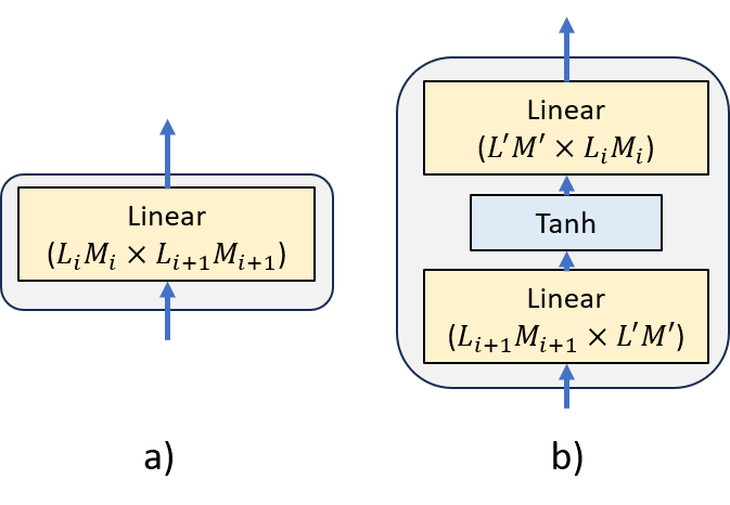
Figure 3: Structure of Linear Kernel. a) Linear kernel, b) Multi-layer Linear Kernel with Tanh activation.

Table 1: Multivariate time series forecasting results with Kernel U-Net. The prediction lengths $T$ are in {96, 192, 336, 720} for all datasets. We note the best results in bold and the second best results in underlined.

Methods		K-U-Net		PatchTST		Nlinear		Dlinear		FEDformer		Autoformer		Informer		Yformer
Metric		MSE	MAE	MSE	MAE	MSE	MAE	MSE	MAE	MSE	MAE	MSE	MAE	MSE	MAE	MSE	MAE
ETTh1	96	0.370	0.393	0.37	0.4	0.374	0.394	0.375	0.399	0.376	0.419	0.449	0.459	0.865	0.713	0.985	0.74
	192	0.404	0.414	0.413	0.429	0.408	0.415	0.405	0.416	0.42	0.448	0.5	0.482	1.008	0.792	1.17	0.855
	336	0.420	0.430	0.422	0.44	0.429	0.427	0.439	0.443	0.459	0.465	0.521	0.496	1.107	0.809	1.208	0.886
	720	0.438	0.454	0.447	0.468	0.44	0.453	0.472	0.49	0.506	0.507	0.514	0.512	1.181	0.865	1.34	0.899
ETTh2	96	0.271	0.335	0.274	0.337	0.277	0.338	0.289	0.353	0.346	0.388	0.358	0.397	3.755	1.525	1.335	0.936
	192	0.332	0.377	0.339	0.379	0.344	0.381	0.383	0.418	0.429	0.439	0.456	0.452	5.602	1.931	1.593	1.021
	336	0.357	0.4	0.329	0.384	0.357	0.4	0.448	0.465	0.496	0.487	0.482	0.486	4.721	1.835	1.444	0.96
	720	0.39	0.438	0.379	0.422	0.394	0.436	0.605	0.551	0.463	0.474	0.515	0.511	3.647	1.625	3.498	1.631
ETTm1	96	0.286	0.342	0.29	0.342	0.306	0.348	0.299	0.343	0.379	0.419	0.505	0.475	0.672	0.571	0.849	0.669
	192	0.330	0.363	0.332	0.369	0.349	0.375	0.335	0.365	0.426	0.441	0.553	0.496	0.795	0.669	0.928	0.724
	336	0.360	0.384	0.366	0.392	0.375	0.388	0.369	0.386	0.445	0.459	0.621	0.537	1.212	0.871	1.058	0.786
	720	0.405	0.412	0.416	0.42	0.433	0.422	0.425	0.421	0.543	0.49	0.671	0.561	1.166	0.823	0.955	0.703
ETTm2	96	0.16	0.245	0.165	0.255	0.167	0.255	0.167	0.26	0.203	0.287	0.255	0.339	0.365	0.453	0.487	0.529
	192	0.215	0.215	0.22	0.292	0.221	0.293	0.224	0.303	0.269	0.328	0.281	0.34	0.533	0.563	0.789	0.705
	336	0.268	0.326	0.274	0.329	0.274	0.327	0.281	0.342	0.325	0.366	0.339	0.372	1.363	0.887	1.256	0.904
	720	0.343	0.379	0.362	0.385	0.368	0.384	0.397	0.421	0.421	0.415	0.433	0.432	3.379	1.338	2.698	1.297
Electricity	96	0.129	0.226	0.129	0.222	0.141	0.237	0.14	0.237	0.193	0.308	0.201	0.317	0.274	0.368	-	-
	192	0.147	0.244	0.147	0.24	0.154	0.248	0.153	0.249	0.201	0.315	0.222	0.334	0.296	0.386	-	-
	336	0.163	0.261	0.163	0.259	0.171	0.265	0.169	0.267	0.214	0.329	0.231	0.338	0.3	0.394	-	-
	720	0.197	0.292	0.197	0.29	0.21	0.297	0.203	0.301	0.246	0.355	0.254	0.361	0.373	0.439	-	-
Traffic	96	0.358	0.253	0.36	0.249	0.41	0.279	0.41	0.282	0.587	0.366	0.613	0.388	0.719	0.391	-	-
	192	0.373	0.262	0.379	0.25	0.423	0.284	0.423	0.287	0.604	0.373	0.616	0.382	0.696	0.379	-	-
	336	0.390	0.271	0.392	0.264	0.435	0.29	0.436	0.296	0.621	0.383	0.622	0.337	0.777	0.42	-	-
	720	0.430	0.292	0.432	0.286	0.464	0.307	0.466	0.315	0.626	0.382	0.66	0.408	0.864	0.472	-	-
Weather	96	0.142	0.195	0.149	0.198	0.182	0.232	0.176	0.237	0.217	0.296	0.266	0.336	0.3	0.384	-	-
	192	0.188	0.244	0.194	0.241	0.225	0.269	0.22	0.282	0.276	0.336	0.307	0.367	0.598	0.544	-	-
	336	0.241	0.284	0.245	0.282	0.271	0.301	0.265	0.319	0.339	0.38	0.359	0.395	0.578	0.523	-	-
	720	0.310	0.333	0.314	0.334	0.338	0.348	0.323	0.362	0.403	0.428	0.419	0.428	1.059	0.741	-	-

3.4 Complexity Analysis

As the K-U-Net is symmetric, we study the complexity of the encoder. Let us suppose that a kernel is receiving a sequence of length $L$ where $L=\prod_{1}^{n}L_{i}$ and all $L_{i}$ are equal. As the patch size in the first layer of Kernel U-Net encoder is $L_{1}$, a kernel module will process $\frac{L}{L_{1}}$ patches of size $L_{1}$. Therefore, the complexity is $O(\frac{L}{L_{1}^{n}}*f(L_{1}))$ where $f(L_{1})$ is the complexity inside the kernel in the function of the patch size $L_{1}$ and $n$ is the index of the layer. In the case of using the linear kernel at the first layer, the complexity is $O(\frac{L}{L_{1}}*L_{1})$= $O(L)$. In the case of using a classic transformer kernel, the complexity is $O(\frac{L}{L_{1}}*L_{1}^{2})$= $O(L*L_{1})$. Let us set $L_{1}=log(L)$, the complexity of the application of such a quadratic calculation kernel is $O(L*log(L))$. Moreover, if we apply the transformer kernel starting from the second layer, the complexity is dramatically reduced to $O(\frac{L}{L_{1}^{2}}*L_{1}^{2})$= $O(L)$. Following the same demonstration, the complexity of using multi-layer linear and LSTM kernels starting from the second layer is also bounded by $O(L)$.

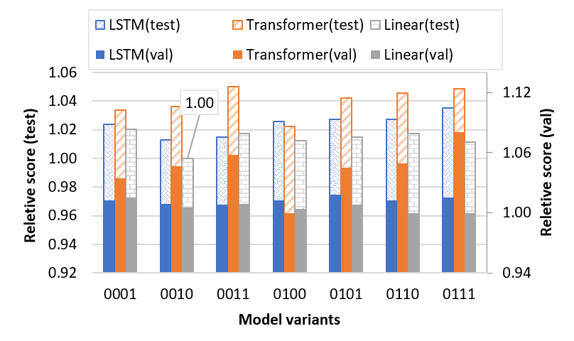
Figure 4: Search result of K-U-Net with Multi-layer Linear, LSTM, Transformer kernels on ETTh1 dataset.

4 Experiments and Results

Datasets.
We conducted experiments on our proposed Kernel U-Net on 7 public datasets, including 4 ETT (Electricity Transformer Temperature) datasets (ETTh1, ETTh2, ETTm1, ETTm2), Weather, Traffic and Electricity. These datasets have been benchmarked and publicly available onWu et al. (2021) and the description of the dataset is available in Zeng et al. (2023)).

Figure 5: Search result of K-U-Net with Multi-layer Linear, LSTM, Transformer kernels on Weather dataset.

Here, we followed the experiment setting in Zeng et al. (2023) and partitioned the data into $[12,4,4]$ months for training, validation, and testing respectively for the ETT dataset. The data is split into $[0.7,0.1,0.2]$ for training, validation, and testing for the Weather, Traffic, and Electricity datasets.

Baselines and Experimental Settings.
We follow the experiment setting in NLinear Zeng et al. (2023) and take $L=\{336,720\}$ step historical data as input then forecast $T\in\{96,192,336,720\}$ step value in the future. We replace the last value normalization with mean value normalization for ETT, Electricity, and Weather datasets, and apply instance normalizationUlyanov et al. (2017) for the Traffic dataset. We use Mean Squared Error (MSE) and Mean Absolute Error (MAE) as mentioned in Wu et al. (2021).

We include recent methods: PatchTSTNie et al. (2023), NLinear, DLinearZeng et al. (2023), FEDformer Zhou et al. (2022), Autoformer Wu et al. (2021), Informer Zhou et al. (2021), LogTrans Li et al. (2019) YformerMadhusudhanan et al. (2023). We merge the result reported in Nie et al. (2023) and Zeng et al. (2023) for taking their best in a supervised setting and execute Yformer in our environment with default parameters in its Github.

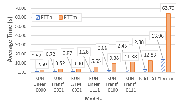
Figure 6: Computation time of K-U-Net, PatchTST and Yformer.

Model Variants Search.
We propose 4 kernels for experiments with K-U-Net on 7 datasets. By replacing a linear kernel at different layers with other types of kernels for searching for variants that adapt the dataset. The variants are noted as ”K-U-Net $<$kernel$>$_$<$replacing_layer$>$ ($<$lookback_window$>$)”. For example, K-U-Net Linear$\_0000(720)$ means that the model is made of linear kernels at all layers and the lookback window size is 720, K-U-Net Transf$\_0100(720)$ means that a transformer kernel replaces the linear kernel at the second layer, K-U-Net Linear$\_0110(720)$ means that multilayer linear kernels replace the kernels at the second and third layers. We compose 16 variants with Multi-layer linear kernels and 7 variants with Transformer and LSTM kernels.

To enumerate all variants that achieve at least once the best result, we report their performance by the average of the top 5 minimum running MSE(Top5MMSE) values on the validation and test set. The search results are reported with a relative score(RS) to the minimum Top5-MMSE:

$$RS(m)=Min_{t\in T}\frac{Top5MMSE(m,t)}{Min_{\{m\in M,l\in L\}}Top5MMSE(m,t,l)}$$

, where $m$ is a model in the models set $M$, $t$ is a forecasting horizon in $T$, $l$ is a look back window in $L$. Relative score notes the best-performed model with 1 and thus helps to identify the high-potential candidates for further fine-tuning examinations.

We observe in Figure 4 that the best variant for ETTh1 dataset is K-U-Net Linear$\_0010$. Comparing the relative score of the K-U-Net of replacing$\_$layer code ($0010$, $0011$), ($0110$, $0111$) and ($0100$, $0101$), we remark that replacing the highest layer with Transformer and LSTM kernel degrades the performance because of overfitting. Furthermore, We observe in Figure 5 that the best variants for the Weather dataset are K-U-Net Linear$\_0110$, K-U-Net LSTM$\_0100$ and K-U-Net Transf$\_0100$. Comparing the relative score of the K-U-Net of replacing$\_$layer code ($0010$, $0110$), ($0011$, $0111$) and ($0001$, $0101$) we remark that replacing the second layer with Transformer and LSTM kernel gains the performance for their expressiveness.

Among candidates in the search phase, we empirically choose 3 variants for fine-tuning experiments with 5 runs. The final result shows that the performance of Kernel U-Net exceeds or meets the state-of-the-art methods in univariate settings and multivariate settings in most cases.

Multivariate time series forecasting result.
We remark that our model improves the MSE performance around $72.92\%$ compared with Yformer and $0.99\%$ compared to PatchTST and NLinear in the multivariate setting (Table 1). It is worth noting that K-U-Net achieves similar results on the Electricity dataset with a variant based on Multilayer linear kernels.

Univariate time series forecasting result.
Additionally, we remark that our model improves the MSE performance around $60.47\%$ compared with Yformer and $6.06\%$ compared to PatchTST and NLinear in the Univariate setting(Table 3). It is worth noting that K-U-Net improves the MSE performance on ETTh2 for $15.67\%$ compared to PatchTST.

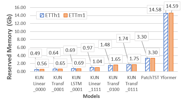
Figure 7: GPU consumation of K-U-Net, PatchTST and Yformer.

Computation Efficiency
We examined the computation efficiency of 4 variants of K-U-Net, PatchTST, and Yformer. We execute the models on the ETTh1 and ETTm1 datasets for 10 epochs and measure the average execution time per epoch and the GPU consumption during the training. The hidden dimension is set to 128 for all models. For fair comparison, PatchTST and Yformer contain 2 layers of Transformer block which equals to K-U-Net_Transf$\_0100$. All experiments are executed on a Tesla V100 GPU in a Google Colab environment. Comparing to the PatchTST, K-U-Net Linear$\_0000$ saves $85.20\%$ and $83.07\%$ memory (Figure 7) and saves $81.82\%$ and $80.55\%$ computation time (Figure 6) on ETTh1 and ETTm1 datasets, K-U-Net_Transf$\_0100$ saves $55.15\%$ and $50.00\%$ memory and saves $28.47\%$ and $26.88\%$ computation time respectively.

5 Conclusion

In this paper, we propose Kernel-U-Net, a highly potential candidate for large-scale time series forecasting tasks. It provides convenience for composing particular models with custom kernels, thereby it adapts well to particular datasets. As an efficient architecture, it accelerates the procedure of searching for appropriate variants. Kernel-U-Net either exceeds or meets the state-of-the-art results in most cases. In the future, we hope to develop more kernels and hope that Kernel U-Net can be useful for other time series tasks such as classification or anomaly detection.

Appendix A Appendix

A.1 Complement Algorithms

The complete algorithm of Kernel U-Net contains creation of Encoder, Decoder (Algorithm 3), Wrapper, and Kernel U-Net(Algorithm 4).

Algorithm 3 Kernel U-Net Decoder

Input: $L_{h}$, $M_{h}$, $[L_{n},...,L_{2}]$, $[L_{n+m},...,L_{n+2}]$, $L_{1}$, $M_{1}$, $[f_{n+m},...,f_{n+2},$ $f_{n},...,f_{2}]$, $[M_{n+m},...,M_{n+2},$ $M_{n},...,M_{2}]$, $L_{1}$, $M_{1}$.

Output: Instance of Kernel U-Net Decoder

  # Define the init function :

  def __init(inputs)__:

  # Create a list of multiples

  L=$[L_{n+m},...,L_{n+2}$ $,L_{n},...,L_{2},L_{1}]$

  # Create first layer

  layers = [KernelWrapper($f_{n+m},$ $1,$ $M_{h},$

  $L_{n+m},$ $M_{n+m}$)]

  # Create intermediate layers

  for  $i$ in $[n+m-1,...,n+2,n,...,2]$ do

           layers.append(KernelWrapper($f_{i},$ $1,M_{i+1}$

           $,L_{i},M_{i})$)

  end for

  # Create last layer

  layers.append(KernelWrapper($f_{2},1,$ $M_{2},$ $L_{1},$ $M_{1})$)

  decoder = nn.Sequential (*layers)

Algorithm 4 Kernel U-Net

Input: $L_{1},M_{1}$, $[,L_{2},...,L_{n},$ $L_{n+2},...,L_{n+m}]$, $[M_{2},...,M_{n},$ $M_{n+2},...,M_{n+m}]$, $[f_{1},f_{2},...,f_{n},$ $f_{n+2},...,f_{n+m}]$, $L_{h}$, $M_{h}$

Output: Instance of Kernel U-Net

  # Define the init function :

  def __init(inputs)__:

  # Initiation of encoder and decoder in K-U-N.

  encoder = KernelUNetEncoder(inputs)

  decoder = KernelUNetDecoder(inputs)

  # Define the forward function :

  def forward(x):

  reshape x to $(B,\prod_{2}^{n}L_{i},L_{1},\prod_{2}^{m}M_{i},M_{1})$

  transpose x to $(B,\prod_{2}^{m}M_{i},\prod_{2}^{n}L_{i},L_{1},M_{1})$

  reshape x to $(B*\prod_{2}^{m}M_{i}*\prod_{2}^{n}L_{i},L_{1},M_{1})$

  # Apply encoder on x

  z = encoder(x)

  for  $i$ in $[1,...,n]$ do

           output = encoder.layers[i]._unet_skip_output

           decoder.layers[$n-i+1$]._unet_skip_input

           = output

  end for

  # Apply decoder on z

  y= decoder(z)

  reshape y to $(B,\prod_{2}^{m}M_{i},\prod_{2}^{n}L_{i},L_{1},M_{1})$

  transpose y to $(B,\prod_{2}^{n}L_{i},L_{1},\prod_{2}^{m}M_{i},M_{1})$

  reshape y to $(B,L,M)$

  return y

A.2 LSTM and Transformer kernels

Transformer kernel
The Vanilla Transformer is made of a layer of positional encoding, blocks that are composed of layers of multiple head attentions, and a linear layer with SoftMax activation. We follow the description in Wen et al. [2023].

Positional encoding (PE).
In a vanilla Transformer, the input sequence is added by a positional encoding vector given by:

$$PE(t)=\left\{\begin{array}[]{ll}sin(\omega it)&ifi\%2=0\\ cos(\omega it)&ifi\%2=1\\ \end{array}\right.$$

, where $\omega i$ is the frequency of waves generated at each dimension. By adding positional information to the input, the transformer can consider the same patterns that occur in different time steps as different patterns.

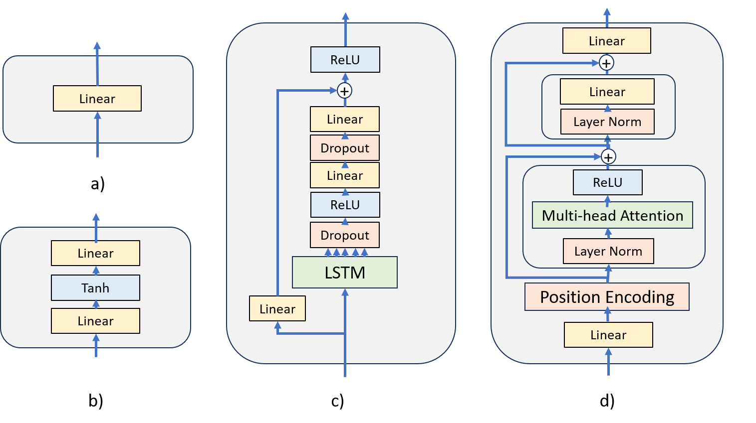
Figure 8: Structure of Kernels a) Linear Kernel, b) Multi layer linear Kernel with Tanh activation, c) LSTM Kernel, d) Transformer Kernel

Multiple head attentions.
With the Query-Key-Value $(QKV)$ model, the scaled dot-product attention used by Transformer is given by

$$Attention(Q,K,V)=Softmax(\frac{QK^{T}}{\sqrt{D_{k}}}))V$$

, where queries $Q\in R^{N\times D_{k}}$ , keys $K\in R^{M\times D_{k}}$ , values $V\in R^{M\times D_{v}}$ , $N,M$ denote the lengths of queries and keys (or values), and $D_{k},D_{v}$ denote the dimensions of keys (or queries) and values.

The multiple attention block contains repeated heads and can be given by

$$MultiHeadAttn(Q,K,V)=Concat(h_{1},...,h_{H})W^{O}$$

, where $h_{i}=Attention(QW_{i}^{Q},KW_{i}^{K},VW_{i}^{V}).$

The transformer kernel in this work (Figure 8) follows the classical structure with 2 additional linear layers. The first linear layer before the Transformer block of size $M_{in}\times M_{out}$ reduces the dimension. The last linear layer is a matrix of size $L_{in}*M_{out}\times L_{out}*M_{out}$ that reduces the input length.

LSTM kernel
The Long Short-term Memory contains 3 gates: Forget Gate $f_{t}$, Input Gate $i_{t}$, Output Gate $o_{t}$. Each gate has a weight matrix $W$ and a bias vector $b$ for the current input $x_{t}$ and the previous hidden state $h_{t-1}$. The next cell state $C_{t}$ is updated by the current activated cell state $C^{\prime}_{t}$. The next hidden state $h_{t}$ is updated by the output gate and the next activated cell state. The formulation of the LSTM cell is as follows:

$f_{t}=\sigma(W_{f}[h_{t-1},x_{t}]+b_{f})$

$i_{t}=\sigma(W_{i}[h_{t-1},x_{t}]+b_{i})$

$C^{\prime}_{t}=tanh(W_{C}[h_{t-1},x_{t}]+b_{C})$

$C_{t}=f_{t}C_{t-1}+i_{t}C^{\prime}_{t}$

$o_{t}=\sigma(W_{o}[h_{t-1},x_{t}]+b_{o})$

$h_{t}=o_{t}tanh(C_{t})$

In our experiments, we add linear layers (Figure 8) that take the flattened output of all hidden states of the LSTM cell for linear combination.

$$Z=W*Flatten([h_{1},...,h_{t}])+b$$

, where $W\in R^{L_{i}*d_{h}}$, $b\in R^{L_{i+1}*M_{i+1}}$ and $d_{h}$ is the dimension of hidden state and $d_{h}=M_{i}$ in general. The residual skip operation aside from the LSTM cell contains a linear layer equivalent to a simple linear kernel discussed in the previous sections.

A.3 Dataset and Experiment

Dataset Statistics

We use 7 popular multivariate datasets for experiments. We create subset Weather(S), Electricity(S), and Traffic(S) from top-left to bottom-right for quick search of K-U-Net variants. The statistic is in noted in Table 2. We refer the description of datasets in Nie et al. [2023]:

• Weather dataset collects 21 meteorological indicators in Germany, such as humidity and air temperature.

• Traffic dataset records the road occupancy rates from different sensors on San Francisco freeways.

• Electricity is a dataset that describes 321 customers’ hourly electricity consumption.

• ETT (Electricity Transformer Temperature) datasets are collected from two different electric transformers labeled with 1 and 2, and each of them contains 2 different resolutions (15 minutes and 1 hour) denoted with m and h.

Table 2: Statistics of popular datasets for experiments.

Datasets	ETTh1	ETTh2	ETTm1	ETTm2	Weather	Traffic	Electricity	Weather(S)	Traffic(S)	Electricity(S)
Features	7	7	7	7	21	862	321	21 (100%)	21 (2.5%)	22 (7%)
Timesteps	17420	17420	69680	69680	52696	17544	26304	10539 (20%)	12280 (70%)	10521 (40%)

Table 3: Univariate time series forecasting results with Kernel U-Net. The prediction lengths $T$ are in {96, 192, 336, 720} for all datasets. We note the best results in bold and the second best in underlined.

Methods		K-U-Net		PatchTST		Nlinear		Dlinear		FEDformer		Autoformer		LogTrans		Yformer
Metric		MSE	MAE	MSE	MAE	MSE	MAE	MSE	MAE	MSE	MAE	MSE	MAE	MSE	MAE	MSE	MAE
ETTh1	96	0.053	0.177	0.055	0.179	0.053	0.177	0.056	0.18	0.079	0.215	0.071	0.206	0.283	0.468	0.211	0.379
	192	0.069	0.205	0.071	0.215	0.069	0.204	0.071	0.204	0.104	0.245	0.114	0.262	0.234	0.409	0.228	0.403
	336	0.076	0.221	0.076	0.22	0.081	0.226	0.098	0.244	0.119	0.27	0.107	0.258	0.386	0.546	0.179	0.355
	720	0.077	0.224	0.087	0.232	0.08	0.226	0.189	0.359	0.127	0.28	0.126	0.283	0.475	0.629	0.260	0.444
ETTh2	96	0.114	0.267	0.129	0.282	0.129	0.278	0.131	0.279	0.128	0.271	0.153	0.306	0.217	0.379	0.240	0.398
	192	0.146	0.306	0.168	0.328	0.169	0.324	0.176	0.329	0.185	0.33	0.204	0.351	0.281	0.429	0.270	0.429
	336	0.157	0.321	0.171	0.336	0.194	0.355	0.209	0.367	0.231	0.378	0.246	0.389	0.293	0.437	0.263	0.422
	720	0.182	0.347	0.223	0.38	0.225	0.381	0.276	0.426	0.278	0.42	0.268	0.409	0.218	0.387	0.264	0.423
ETTm1	96	0.026	0.122	0.026	0.121	0.026	0.122	0.028	0.123	0.033	0.14	0.056	0.183	0.049	0.171	0.211	0.393
	192	0.039	0.15	0.039	0.15	0.039	0.149	0.045	0.156	0.058	0.186	0.081	0.216	0.157	0.317	0.262	0.42
	336	0.051	0.173	0.053	0.173	0.052	0.172	0.061	0.182	0.071	0.209	0.076	0.218	0.289	0.459	0.424	0.559
	720	0.068	0.202	0.073	0.206	0.073	0.207	0.08	0.21	0.102	0.25	0.11	0.267	0.43	0.579	0.413	0.552
ETTm2	96	0.062	0.182	0.065	0.187	0.063	0.182	0.063	0.183	0.063	0.189	0.065	0.189	0.075	0.208	0.128	0.275
	192	0.089	0.224	0.093	0.231	0.09	0.223	0.092	0.227	0.102	0.245	0.118	0.256	0.129	0.275	0.155	0.308
	336	0.114	0.259	0.121	0.266	0.117	0.259	0.119	0.261	0.13	0.279	0.154	0.305	0.154	0.302	0.208	0.358
	720	0.156	0.312	0.171	0.322	0.17	0.318	0.175	0.32	0.178	0.325	0.182	0.335	0.16	0.321	0.261	0.405

Table 4: Comparison of 16 variants of Linear K-U-Net in baseline setting and without using Skip connection(-Skip), Random Erase(-RE), Chanel Independence(-CI). The prediction lengths $T$ are in {96, 192, 336, 720} for all datasets. We note the best results in bold and the second best results in underlined for minimum score(Min) and average score(Mean).

Method		Min (Base)		Min (-Skip)		Min (-RE)		Min (-CI)		Mean (Base)		Mean (-Skip)		Mean (-RE)		Mean (-CI)
Metric		MSE	Top5-
MMSE	MSE	Top5-
MMSE	MSE	Top5-
MMSE	MSE	Top5-
MMSE	MSE	Top5-
MMSE	MSE	Top5-
MMSE	MSE	Top5-
MMSE	MSE	Top5-
MMSE
ETTh1	96	0.368	0.368	0.375	0.375	0.370	0.369	0.459	0.451	0.376	0.374	0.393	0.385	0.377	0.373	0.488	0.483
	192	0.404	0.402	0.412	0.413	0.402	0.402	0.506	0.495	0.409	0.407	0.423	0.423	0.411	0.407	0.551	0.538
	336	0.423	0.421	0.443	0.441	0.427	0.422	0.535	0.519	0.443	0.430	0.489	0.455	0.442	0.431	0.581	0.549
	720	0.457	0.439	0.461	0.453	0.461	0.438	0.629	0.576	0.492	0.472	0.531	0.515	0.488	0.470	0.690	0.598
ETTh2	96	0.274	0.272	0.273	0.273	0.274	0.273	0.423	0.397	0.302	0.287	0.299	0.290	0.300	0.286	0.458	0.415
	192	0.336	0.353	0.337	0.355	0.336	0.354	0.414	0.442	0.370	0.375	0.376	0.382	0.372	0.374	0.445	0.474
	336	0.361	0.361	0.364	0.364	0.362	0.361	0.412	0.422	0.402	0.384	0.404	0.392	0.399	0.384	0.428	0.444
	720	0.398	0.394	0.397	0.397	0.395	0.394	0.453	0.456	0.451	0.418	0.459	0.436	0.444	0.420	0.468	0.519
ETTm1	96	0.288	0.284	0.289	0.290	0.288	0.284	0.321	0.318	0.296	0.292	0.303	0.298	0.296	0.291	0.346	0.333
	192	0.324	0.327	0.325	0.324	0.326	0.324	0.359	0.358	0.335	0.331	0.341	0.336	0.334	0.331	0.383	0.373
	336	0.359	0.358	0.353	0.354	0.359	0.357	0.391	0.391	0.366	0.363	0.374	0.368	0.366	0.362	0.418	0.406
	720	0.408	0.404	0.403	0.403	0.409	0.403	0.452	0.447	0.418	0.411	0.419	0.413	0.418	0.410	0.478	0.467
ETTm2	96	0.162	0.162	0.162	0.161	0.163	0.161	0.213	0.204	0.168	0.165	0.170	0.165	0.168	0.164	0.228	0.210
	192	0.218	0.217	0.216	0.215	0.217	0.216	0.298	0.274	0.228	0.223	0.229	0.224	0.228	0.222	0.318	0.286
	336	0.270	0.268	0.268	0.267	0.265	0.265	0.372	0.345	0.283	0.277	0.281	0.277	0.284	0.272	0.394	0.356
	720	0.342	0.349	0.343	0.347	0.343	0.347	0.410	0.408	0.354	0.361	0.351	0.361	0.364	0.356	0.434	0.421
Average decrease				+0.42%	+0.77%	+0.03%	-0.20%	+24.19%	+21.45%			+2.24%	+2.30%	+0.03%	-0.32%	+25.92%	+23.72%

Experiment details

We use a 4-layer K-U-Net for experiments. The list of multiples are respectively [4, 4, 3, 7] and [4, 6, 6, 5] for look-back windows $L$ and forecasting horizons $T$ in {336, 720}. Remark that $T$ is fixed to be 336 for shorter forecasting cases. The bottom patch length is 4 and its width is 1 as we follow the Channel-Independent (CI) setting in Zeng et al. [2023]. In case of not using CI, the patch width equals to feature size. The hidden dimensions are 128 for multivariate and univariate tasks in general, except that they are 256 on the Traffic dataset. The learning rate is selected in $[0.00005,0.001]$ depending on the dataset. The training epoch is 50 and the patience of early stopping is 10 in general.

We apply weighted early stopping where the triggering MSE (TMSE) is computed with $TMSE_{e+1}=\tau*TMSE_{e}+(1-\tau)*VMSE_{e}$ , where $\tau$ is a hyper-parameter to be set, $e$ is the index of the episode, and VMSE is the running MSE on a validation set. The parameter $\tau$ sets the sensitivity of early stopping and is empirically selected. In general, it is set to be 0.9 in the variants searching stage and 0.5 in the fine-tuning stage.

The MSE loss function is defined with $:\mathcal{L}=\mathbb{E}_{\boldsymbol{x}}\frac{1}{B*M}\sum_{i=1}^{B*M}\left\|\hat{\boldsymbol{x}}_{L+1:L+T}^{(i)}-\boldsymbol{x}_{L+1:L+T}^{(i)}\right\|_{2}^{2}$ , where $B$ is the batch size and $M$ is the multiple of feature size unit of time series.

A.4 Search of model variants

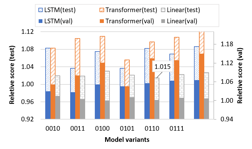
(b) ETTh2

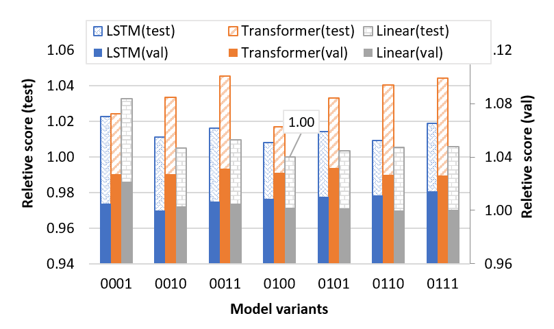
(c) ETTm1

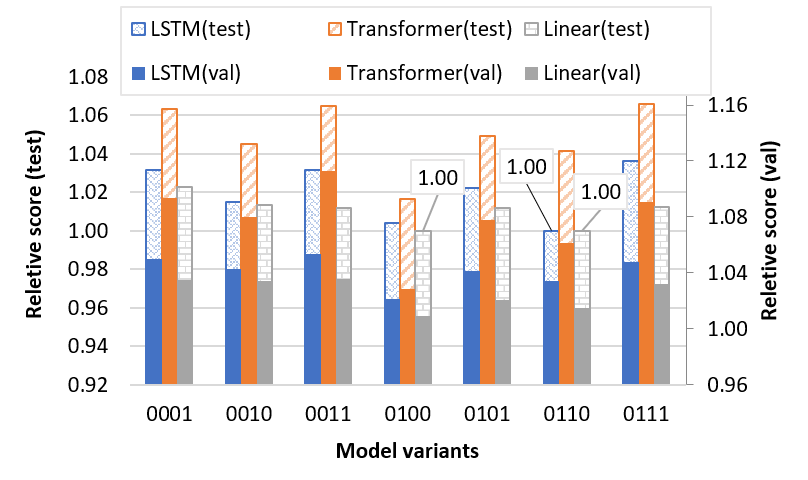
(d) ETTm2

(e) Weather

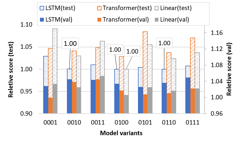
(f) Weather(S)

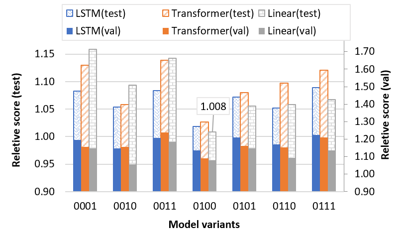
(g) Electricity(S)

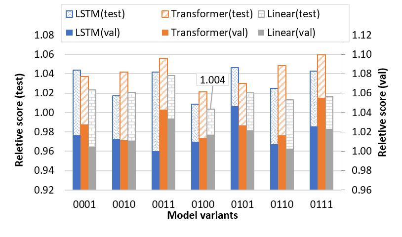
(h) Traffic(S)

Figure 9: Search result of K-U-Net with Multi-layer Linear, LSTM, Transformer kernels on validation and test set.

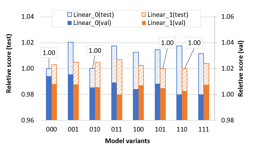
(a) ETTh1

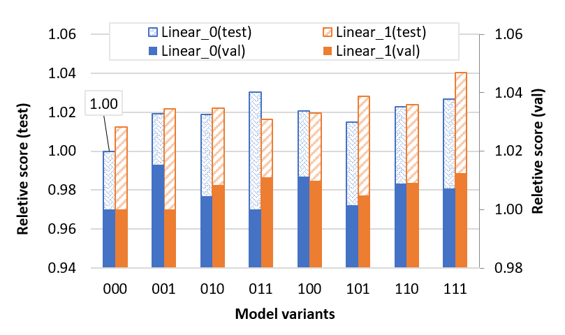
(b) ETTh2

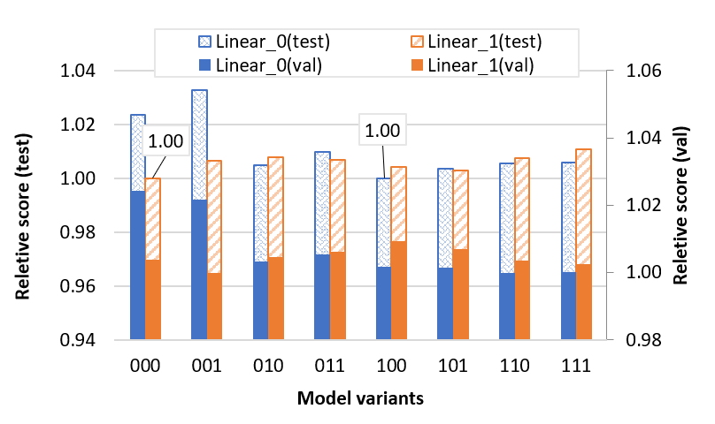
(c) ETTm1

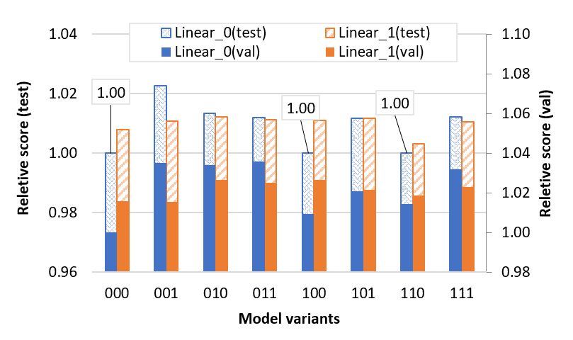
(d) ETTm2

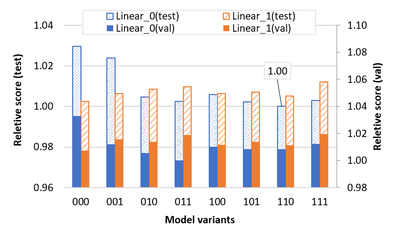
(e) Weather

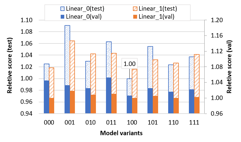
(f) Weather(S)

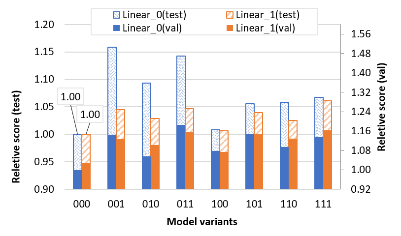
(g) Electricity(S)

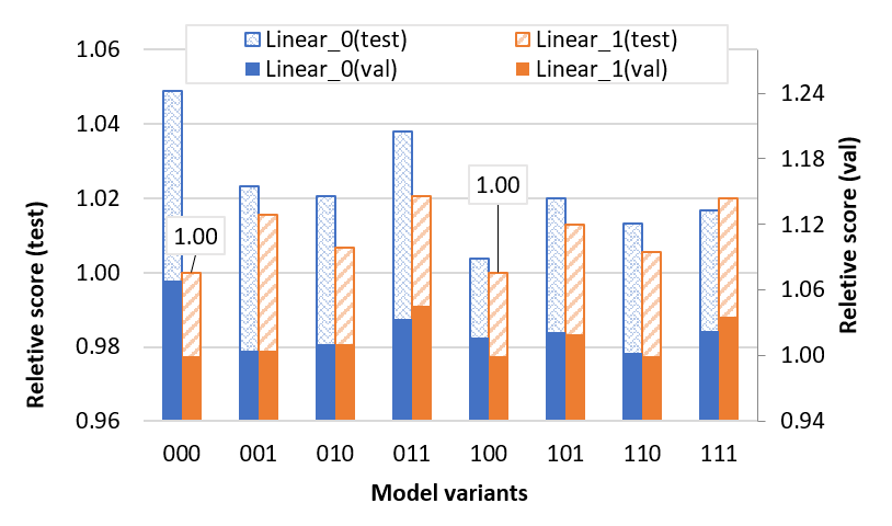
(h) Traffic(S)

Figure 10: Search result of K-U-Net with Multi-layer Linear kernels on validation and test set.

We searched 30 variants of K-U-Net across Linear_[0000,…,1111] and {LSTM, Transformer}_[0100,…,1111] for the ETT, Weather datasets and 3 subsets. The lookback window is typically 720, and we additionally tested a version of 336 on the ETT dataset. The result is reported with the average of running Top5 Minimum MSE (Top5MMSE) on the validation and test set in a single run. This measures the extreme performance of a variant and its potential in the fine-tuning stage. We use relative score (RS) to locate best-performed variants (i.g. $RS=1$ means that it’s the best among all candidates). We plot the RS of variants of 5 datasets in Figures 9 and Figures 10.

Based on the search result, We note that Linear and Multilayer linear kernels are more adapted in the ETT dataset than our Transformer and LSTM kernels. We remark that K-U-Net Linear_1000 is outstanding in the Electricity (S) dataset and thus selected for full examination.

A.5 Result of selected variants

In Table 5 6 7, we note selected models that are examined prudently with 5 runs in a fine-tuned context and measures with average MSE and MAE. We include the Table 9 showing that K-U-Net has a small standard deviation error across 5 random runs.

A.6 Result of univariate time series forecasting

The experiment of univariate time series forecasting task predicts the target feature is the ”oil temperature” on ETT datasets. We remark that our model improves the MSE performance around $60.47\%$ compared with Yformer and $6.06\%$ compared to PatchTST and NLinear in the Univariate setting(Table 3). It is worth noting that K-U-Net improves the MSE performance on ETTh2 for $15.67\%$ in the Univariate setting compared to PatchTST.

Appendix B Ablation Study

For studying the roles of skip connection in K-U-Net, Random Erase, and Chanel Independence, we use the Minimum Top5 average MSE (Min Top5MMSE) to measure the extreme performance and the Mean Top5MMSE to measure the average performance. For instance Normalisation, we only show the comparison with Mean Normalization with the Traffic dataset because the improvement is evident.

Table 5: Fine-tuned multivariate time series forecasting results with Kernel U-Net on datasets ETTh and ETTm. The prediction lengths $T$ are in {96, 192, 336, 720} for all datasets. We note the best results in bold.

Method		K-U-Net
Linear_0000
(336)		K-U-Net
Linear_0000
(720)		K-U-Net
Linear_1100
(720)		MIN		PatchTST
Metric		MSE	MAE	MSE	MAE	MSE	MAE	MSE	MAE	MSE	MAE
ETTh1	96	0.372	0.393	0.377	0.401	0.370	0.407	0.370	0.393	0.370	0.400
	192	0.405	0.414	0.413	0.424	0.404	0.433	0.404	0.414	0.413	0.429
	336	0.431	0.430	0.444	0.444	0.420	0.445	0.420	0.430	0.422	0.440
	720	0.438	0.454	0.457	0.471	0.482	0.490	0.438	0.454	0.447	0.468

Method		K-U-Net
Linear_0000
(336)		K-U-Net
Linear_0000
(720)		K-U-Net
Linear_0001
(720)		MIN		PatchTST
Metric		MSE	MAE	MSE	MAE	MSE	MAE	MSE	MAE	MSE	MAE
ETTh2	96	0.273	0.335	0.271	0.336	0.286	0.342	0.271	0.335	0.274	0.337
	192	0.336	0.377	0.332	0.377	0.354	0.384	0.332	0.377	0.339	0.379
	336	0.360	0.401	0.357	0.403	0.388	0.413	0.357	0.401	0.329	0.384
	720	0.395	0.435	0.394	0.442	0.420	0.447	0.394	0.435	0.379	0.422

Method		K-U-Net
Linear_0000
(336)		K-U-Net
Linear_0000
(720)		K-U-Net
Linear_1000
(720)		MIN		PatchTST
Metric		MSE	MAE	MSE	MAE	MSE	MAE	MSE	MAE	MSE	MAE
ETTm1	96	0.301	0.343	0.310	0.351	0.286	0.342	0.286	0.342	0.290	0.342
	192	0.336	0.363	0.338	0.368	0.330	0.371	0.330	0.363	0.332	0.369
	336	0.371	0.384	0.367	0.385	0.360	0.393	0.360	0.384	0.366	0.392
	720	0.427	0.416	0.417	0.412	0.405	0.420	0.405	0.412	0.416	0.420

Method		K-U-Net
Linear_0000
(336)		K-U-Net
Linear_0000
(720)		K-U-Net
Linear_0110
(720)		MIN		PatchTST
Metric		MSE	MAE	MSE	MAE	MSE	MAE	MSE	MAE	MSE	MAE
ETTm2	96	0.164	0.253	0.161	0.252	0.165	0.256	0.161	0.252	0.165	0.255
	192	0.219	0.290	0.216	0.290	0.225	0.296	0.216	0.290	0.220	0.292
	336	0.273	0.326	0.268	0.326	0.275	0.332	0.268	0.326	0.274	0.329
	720	0.367	0.383	0.350	0.379	0.343	0.380	0.343	0.379	0.362	0.385

Table 6: Fine-tuned multivariate time series forecasting results with Kernel U-Net on datasets Electricity, Weather and Traffic. The prediction lengths $T$ are in {96, 192, 336, 720} for all datasets. We note the best results in bold.

Method		K-U-Net
Linear_0000
(720)		K-U-Net
Linear_1110
(720)		K-U-Net
Linear_1000
(720)		MIN		PatchTST
Metric		MSE	MAE	MSE	MAE	MSE	MAE	MSE	MAE	MSE	MAE
Electricity	96	0.138	0.237	0.134	0.232	0.129	0.226	0.129	0.226	0.129	0.222
	192	0.153	0.250	0.152	0.249	0.147	0.244	0.147	0.244	0.147	0.240
	336	0.171	0.269	0.167	0.264	0.163	0.261	0.163	0.261	0.163	0.259
	720	0.213	0.305	0.203	0.300	0.197	0.292	0.197	0.292	0.197	0.290

Method		K-U-Net
Linear_0000
(720)		K-U-Net
Transf_0001
(720)		K-U-Net
LSTM_0001
(720)		MIN		PatchTST
Metric		MSE	MAE	MSE	MAE	MSE	MAE	MSE	MAE	MSE	MAE
Traffic	96	0.412	0.280	0.399	0.262	0.358	0.253	0.358	0.253	0.360	0.249
	192	0.425	0.287	0.415	0.278	0.373	0.262	0.373	0.262	0.379	0.250
	336	0.438	0.294	0.424	0.295	0.390	0.271	0.390	0.271	0.392	0.264
	720	0.458	0.314	0.465	0.309	0.430	0.292	0.430	0.292	0.432	0.286

Method		K-U-Net
Linear_0110
(720)		K-U-Net
Transf_0001
(720)		K-U-Net
LSTM_0100
(720)		MIN		PatchTST
Metric		MSE	MAE	MSE	MAE	MSE	MAE	MSE	MAE	MSE	MAE
Weather	96	0.146	0.201	0.146	0.200	0.142	0.195	0.142	0.195	0.149	0.198
	192	0.190	0.245	0.192	0.246	0.188	0.244	0.188	0.244	0.194	0.241
	336	0.241	0.284	0.242	0.287	0.242	0.286	0.241	0.284	0.245	0.282
	720	0.310	0.333	0.310	0.336	0.316	0.341	0.310	0.333	0.314	0.334

B.1 Instance Normalisation and Mean Normalisation

Instance normalization contains a step of substruction with the average value of the input sequence and a division of its standard deviation. It computes reversely the multiplication of its standard deviation and the addition of the average value after the output of the model. Mean normalization removes the division and multiplication step of the standard deviation of instance normalization to avoid introducing noises into the dataset. We employed the mean normalization as the preprocessing step for most experiments except those with instance normalization on traffic datasets. The comparison in Table 8 shows that Instance Normalization improves the MSE by 3.89% for a K-U-Net LSTM_0001 on traffic datasets.

Table 7: Fine-tuned univariate time series forecasting results with Kernel U-Net on datasets ETTh and ETTm. The prediction lengths $T$ are in {96, 192, 336, 720} for all datasets. We note the best results in bold.

Method		K-U-Net
Linear_0000
(336)		K-U-Net
Linear_1111
(336)		MIN		PatchTST		Nlinear
Metric		MSE	MAE	MSE	MAE	MSE	MAE	MSE	MAE	MSE	MAE
ETTh1	96	0.053	0.177	0.054	0.182	0.053	0.177	0.055	0.179	0.053	0.177
	192	0.069	0.205	0.079	0.219	0.069	0.205	0.071	0.215	0.069	0.204
	336	0.076	0.222	0.076	0.221	0.076	0.221	0.076	0.22	0.081	0.226
	720	0.077	0.224	0.078	0.226	0.077	0.224	0.087	0.232	0.08	0.226

Method		K-U-Net
Linear_0110
(336)		K-U-Net
Linear_1100
(336)		MIN		PatchTST		Nlinear
Metric		MSE	MAE	MSE	MAE	MSE	MAE	MSE	MAE	MSE	MAE
ETTh2	96	0.114	0.267	0.121	0.272	0.114	0.267	0.129	0.282	0.129	0.278
	192	0.146	0.306	0.161	0.317	0.146	0.306	0.168	0.328	0.169	0.324
	336	0.157	0.321	0.178	0.340	0.157	0.321	0.171	0.336	0.194	0.355
	720	0.192	0.355	0.182	0.347	0.182	0.347	0.223	0.38	0.225	0.381

Method		K-U-Net
Linear_0000
(336)		K-U-Net
Linear_0000
(720)		MIN		PatchTST		Nlinear
Metric		MSE	MAE	MSE	MAE	MSE	MAE	MSE	MAE	MSE	MAE
ETTm1	96	0.026	0.121	0.026	0.122	0.026	0.121	0.026	0.121	0.026	0.122
	192	0.038	0.149	0.039	0.150	0.038	0.149	0.039	0.15	0.039	0.149
	336	0.051	0.173	0.051	0.174	0.051	0.173	0.053	0.173	0.052	0.172
	720	0.072	0.206	0.068	0.203	0.068	0.203	0.073	0.206	0.073	0.207

Method		K-U-Net
Linear_0000
(336)		K-U-Net
Linear_1000
(720)		MIN		PatchTST		Nlinear
Metric		MSE	MAE	MSE	MAE	MSE	MAE	MSE	MAE	MSE	MAE
ETTm2	96	0.063	0.182	0.062	0.183	0.062	0.182	0.065	0.187	0.063	0.182
	192	0.090	0.224	0.089	0.227	0.089	0.224	0.093	0.231	0.09	0.223
	336	0.116	0.259	0.114	0.263	0.114	0.259	0.121	0.266	0.117	0.259
	720	0.170	0.319	0.156	0.312	0.156	0.312	0.171	0.322	0.17	0.318

Table 8: Comparison of Mean Normalization(+MN) and Instance Normalization (+IN) on Traffic dataset. We note the best results in bold..

Methods		K-U-Net (+MN)
LSTM_0001
(720)		K-U-Net (+IN)
LSTM_0001
(720)
Metric		MSE	MAE	MSE	MAE
Traffic	96	0.375	0.264	0.360	0.252
	192	0.393	0.275	0.377	0.263
	336	0.406	0.280	0.389	0.270
	720	0.442	0.296	0.427	0.290

Table 9: MSE and standard deviation of K-U-Net across 5 random runs.

Method		K-U-Net
LSTM_0001
(720)		Method		K-U-Net
LSTM_0100
(720)		Method		K-U-Net
Linear_1000
(720)
Metric		MSE		Metric		MSE		Metric		MSE
Traffic	96	0.35761	±0.00042	Weather	96	0.14200	±0.00016	ETTm1	96	0.28600	±0.00056
	192	0.37266	±0.00056		192	0.18782	±0.00078		192	0.32996	±0.00204
	336	0.39030	±0.00135		336	0.24164	±0.00139		336	0.35979	±0.00092
	720	0.42970	±0.00078		720	0.31646	±0.00198		720	0.40539	±0.00128

B.2 Skip Connection,

Skip Connection in the U-Net is used for passing information from the encoder to the same level on its symmetric decoder. As the size of the hidden vector is reduced during passage in the encoder, skip connection helps keep the low-level features and allows the decoder to mix with high-level information. We conduct experiments to understand the role of skip connection in the K-U-Net. The result in Table 4 shows that removing the skip connection degrades the Min Top5MMSE score for $0.77\%$ on average and especially $3.19\%$ on the ETTh1 dataset. Additionally, it degrades $2.30\%$ Mean Top5MMSE on average and especially $5.42\%$ on the ETTh1 dataset.

B.3 Comparison of Chanel Independent and Chanel Mixing

Chanel Independent was an inherited choice from Zeng et al. [2023]. It avoids introducing noises that degrade the performance across different features. In this experiment, we compare the channel-independent(CI) strategy and the channel-mixing strategy. In K-U-Net, setting input and output dimension to 1 implies a channel-independent strategy, while setting to feather size (7 for the ETT dataset) means a channel-mixing strategy. As We observe in Table 4, removing CI degrades the Min Top MMSE score for $21.45\%$ and the Min Top5MMSE score for $23.72\%$.

B.4 Comparison of Random Erasing

Random Erasing augments the dataset by masking partially the input. In this experiment, we studied the role of random erasing in time series forecasting settings. We observe in Table 4 that removing Random Erasing degrades the Min Top5MMSE score for $0.2\%~{}0.32\%$, which is not as evident as the Skip Connection and Channel Independent strategy.

(a) ETTh1

References

- Asres et al. [2022] Mulugeta Weldezgina Asres, Grace Cummings, Aleko Khukhunaishvili, Pavel Parygin, Seth I. Cooper, David Yu, Jay Dittmann, and Christian W. Omlin. Long horizon anomaly prediction in multivariate time series with causal autoencoders. PHM Society European Conference, 7(1):21–31, 2022.
- Azar et al. [2022] Joseph Azar, Gaby Bou Tayeh, Abdallah Makhoul, and Raphaël Couturier. Efficient lossy compression for iot using sz and reconstruction with 1d u-net. Mob. Netw. Appl., 27(3):984–996, jun 2022.
- Cao et al. [2023] Hu Cao, Yueyue Wang, Joy Chen, Dongsheng Jiang, Xiaopeng Zhang, Qi Tian, and Manning Wang. Swin-unet: Unet-like pure transformer for medical image segmentation. In Leonid Karlinsky, Tomer Michaeli, and Ko Nishino, editors, Computer Vision – ECCV 2022 Workshops, pages 205–218. Springer Nature Switzerland, 2023.
- Deng et al. [2009] Jia Deng, R. Socher, Li Fei-Fei, Wei Dong, Kai Li, and Li-Jia Li. Imagenet: A large-scale hierarchical image database. In 2009 IEEE Conference on Computer Vision and Pattern Recognition(CVPR), volume 00, pages 248–255, 06 2009.
- Dosovitskiy et al. [2021] Alexey Dosovitskiy, Lucas Beyer, Alexander Kolesnikov, Dirk Weissenborn, Xiaohua Zhai, Thomas Unterthiner, Mostafa Dehghani, Matthias Minderer, Georg Heigold, Sylvain Gelly, Jakob Uszkoreit, and Neil Houlsby. An image is worth 16x16 words: Transformers for image recognition at scale. In 9th International Conference on Learning Representations, ICLR 2021, Virtual Event, Austria, May 3-7, 2021, 2021.
- Du et al. [2015] Yong Du, Wei Wang, and Liang Wang. Hierarchical recurrent neural network for skeleton based action recognition. In Proceedings of the IEEE Conference on Computer Vision and Pattern Recognition, pages 1110–1118, 2015.
- Duan et al. [2022] Ziheng Duan, Haoyan Xu, Yueyang Wang, Yida Huang, Anni Ren, Zhongbin Xu, Yizhou Sun, and Wei Wang. Multivariate time-series classification with hierarchical variational graph pooling. Neural Networks, 154:481–490, 2022.
- Han et al. [2022] Ning Han, Li Zhou, Zhengmao Xie, Jingli Zheng, and Liuxin Zhang. Multi-level u-net network for image super-resolution reconstruction. Displays, 73:102192, 2022.
- Hewage et al. [2020] Pradeep Hewage, Ardhendu Behera, Marcello Trovati, Ella Pereira, Morteza Ghahremani, Francesco Palmieri, and Yonghuai Liu. Temporal convolutional neural (TCN) network for an effective weather forecasting using time-series data from the local weather station. Soft Computing, 24(21):16453–16482, 2020.
- Hong and Yoon [2017] Jeonghan Hong and Junho Yoon. Multivariate time-series classification of sleep patterns using a hybrid deep learning architecture. In 2017 IEEE 19th International Conference on e-Health Networking, Applications and Services (Healthcom), pages 1–6, 2017.
- Khandelwal et al. [2015] Ina Khandelwal, Ratnadip Adhikari, and Ghanshyam Verma. Time series forecasting using hybrid ARIMA and ANN models based on DWT decomposition. Procedia Computer Science, 48:173–179, 2015.
- Kong et al. [2017] Weicong Kong, Z.Y. Dong, Youwei Jia, David Hill, Yan Xu, and Yuan Zhang. Short-term residential load forecasting based on LSTM recurrent neural network. IEEE Transactions on Smart Grid, PP:1–1, 2017.
- Kowsari et al. [2017] Kamran Kowsari, Donald E. Brown, Mojtaba Heidarysafa, Kiana Jafari Meimandi, Matthew S. Gerber, and Laura E. Barnes. HDLTex: Hierarchical deep learning for text classification. In 2017 16th IEEE International Conference on Machine Learning and Applications (ICMLA), pages 364–371, 2017.
- Lai et al. [2018] Guokun Lai, Wei-Cheng Chang, Yiming Yang, and Hanxiao Liu. Modeling long- and short-term temporal patterns with deep neural networks. In The 41st International ACM SIGIR Conference on Research & Development in Information Retrieval, SIGIR ’18, page 95–104, New York, NY, USA, 2018. Association for Computing Machinery.
- Li et al. [2019] Shiyang Li, Xiaoyong Jin, Yao Xuan, Xiyou Zhou, Wenhu Chen, Yu-Xiang Wang, and Xifeng Yan. Enhancing the Locality and Breaking the Memory Bottleneck of Transformer on Time Series Forecasting, page 11. Curran Associates Inc., Red Hook, NY, USA, 2019.
- Liu et al. [2021] Ze Liu, Yutong Lin, Yue Cao, Han Hu, Yixuan Wei, Zheng Zhang, Stephen Lin, and Baining Guo. Swin transformer: Hierarchical vision transformer using shifted windows. In 2021 IEEE/CVF International Conference on Computer Vision (ICCV), pages 9992–10002. IEEE, 2021.
- Liu et al. [2022a] Shizhan Liu, Hang Yu, Cong Liao, Jianguo Li, Weiyao Lin, Alex X Liu, and Schahram Dustdar. Pyraformer: Low-complexity pyramidal attention for long-range time series modeling and forecasting. In International Conference on Learning Representations, 2022.
- Liu et al. [2022b] Yong Liu, Haixu Wu, Jianmin Wang, and Mingsheng Long. Non-stationary transformers: Exploring the stationarity in time series forecasting. Advances in Neural Information Processing Systems, 2022.
- Madhusudhanan et al. [2023] Kiran Madhusudhanan, Johannes Burchert, Nghia Duong-Trung, Stefan Born, and Lars Schmidt-Thieme. U-net inspired transformer architecture for far horizon time series forecasting. In Machine Learning and Knowledge Discovery in Databases: European Conference, ECML PKDD 2022, Grenoble, France, September 19–23, 2022, Proceedings, Part VI, page 36–52, Berlin, Heidelberg, 2023. Springer-Verlag.
- Nie et al. [2023] Yuqi Nie, Nam H. Nguyen, Phanwadee Sinthong, and Jayant Kalagnanam. A time series is worth 64 words: Long-term forecasting with transformers. International Conference on Learning Representations, 2023.
- Perslev et al. [2019] Mathias Perslev, Michael Jensen, Sune Darkner, Poul Jø rgen Jennum, and Christian Igel. U-time: A fully convolutional network for time series segmentation applied to sleep staging. In Advances in Neural Information Processing Systems, volume 32. Curran Associates, Inc., 2019.
- Persson et al. [2017] Caroline Persson, Peder Bacher, Takahiro Shiga, and Henrik Madsen. Multi-site solar power forecasting using gradient boosted regression trees. Solar Energy, 150:423–436, 2017.
- Ronneberger et al. [2015] Olaf Ronneberger, Philipp Fischer, and Thomas Brox. U-net: Convolutional networks for biomedical image segmentation. In Nassir Navab, Joachim Hornegger, William M. Wells, and Alejandro F. Frangi, editors, Medical Image Computing and Computer-Assisted Intervention – MICCAI 2015, pages 234–241. Springer International Publishing, 2015.
- Tokgöz and Ünal [2018] Alper Tokgöz and Gözde Ünal. A RNN based time series approach for forecasting turkish electricity load. In 2018 26th Signal Processing and Communications Applications Conference (SIU), pages 1–4, 2018.
- Ulyanov et al. [2017] Dmitry Ulyanov, Andrea Vedaldi, and Victor Lempitsky. Instance normalization: The missing ingredient for fast stylization, 2017.
- Vaswani et al. [2017] Ashish Vaswani, Noam Shazeer, Niki Parmar, Jakob Uszkoreit, Llion Jones, Aidan N Gomez, Łukasz Kaiser, and Illia Polosukhin. Attention is all you need. In I. Guyon, U. Von Luxburg, S. Bengio, H. Wallach, R. Fergus, S. Vishwanathan, and R. Garnett, editors, Advances in Neural Information Processing Systems, volume 30. Curran Associates, Inc., 2017.
- Wen et al. [2023] Qingsong Wen, Tian Zhou, Chaoli Zhang, Weiqi Chen, Ziqing Ma, Junchi Yan, and Liang Sun. Transformers in time series: A survey. In International Joint Conference on Artificial Intelligence(IJCAI), 2023.
- Wu et al. [2021] Haixu Wu, Jiehui Xu, Jianmin Wang, and Mingsheng Long. Autoformer: Decomposition transformers with auto-correlation for long-term series forecasting. In M. Ranzato, A. Beygelzimer, Y. Dauphin, P. S. Liang, and J. Wortman Vaughan, editors, Advances in Neural Information Processing Systems, volume 34, pages 22419–22430. Curran Associates, Inc., 2021.
- Xiao and Liu [2016] Minguang Xiao and Cong Liu. Semantic relation classification via hierarchical recurrent neural network with attention. In Yuji Matsumoto and Rashmi Prasad, editors, Proceedings of COLING 2016, the 26th International Conference on Computational Linguistics: Technical Papers, pages 1254–1263. The COLING 2016 Organizing Committee, 2016.
- Zeng et al. [2023] Ailing Zeng, Muxi Chen, Lei Zhang, and Qiang Xu. Are transformers effective for time series forecasting? In Proceedings of the AAAI Conference on Artificial Intelligence, 2023.
- Zhang et al. [2023] Kai Zhang, Yawei Li, Jingyun Liang, Jiezhang Cao, Yulun Zhang, Hao Tang, Deng-Ping Fan, Radu Timofte, and Luc Van Gool. Practical blind image denoising via swin-conv-UNet and data synthesis. Mach. Intell. Res., 2023.
- Zhou et al. [2021] Haoyi Zhou, Shanghang Zhang, Jieqi Peng, Shuai Zhang, Jianxin Li, Hui Xiong, and Wancai Zhang. Informer: Beyond efficient transformer for long sequence time-series forecasting. In The Thirty-Fifth AAAI Conference on Artificial Intelligence, AAAI 2021, Virtual Conference, volume 35, pages 11106–11115. AAAI Press, 2021.
- Zhou et al. [2022] Tian Zhou, Ziqing Ma, Qingsong Wen, Xue Wang, Liang Sun, and Rong Jin. FEDformer: Frequency enhanced decomposed transformer for long-term series forecasting. In Proceedings of the 39th International Conference on Machine Learning, pages 27268–27286. PMLR, 2022. issns: 2640-3498.
- Çiçek et al. [2016] Özgün Çiçek, Ahmed Abdulkadir, Soeren S. Lienkamp, Thomas Brox, and Olaf Ronneberger. 3d u-net: Learning dense volumetric segmentation from sparse annotation. In International Conference on Medical Image Computing and Computer-Assisted Intervention, 2016.