Penalty Parameter Selection in Deconvolution by Estimating the Risk for a Smaller Sample Size

Abstract

We address the choice of penalty parameter in the Smoothness-Penalized Deconvolution (SPeD) method of estimating a probability density under additive measurement error. Cross-validation gives an unbiased estimate of the risk (for the present sample size $n$) with a given penalty parameter, and this function can be minimized as a function of the penalty parameter. Least-squares cross-validation, which has been proposed for the similar Deconvoluting Kernel Density Estimator (DKDE), performs quite poorly for SPeD. We instead estimate the risk function for a smaller sample size $n_{1}<n$ with a given penalty parameter, using this to choose the penalty parameter for sample size $n_{1}$, and then use the asymptotics of the optimal penalty parameter to choose for sample size $n$. In a simulation study, we find that this has dramatically better performance than cross-validation, is an improvement over a SURE-type method previously proposed for this estimator, and compares favorably to the classic DKDE with its recommended plug-in method. We prove that the maximum error in estimating the risk function is of smaller order than its optimal rate of convergence.

Keywords: deconvolution, bandwidth selection, density estimation

1 Introduction and Setting

Suppose $X$ has unknown pdf $f$, $E$ has known pdf $g$, and $X$ and $E$ are independent. Then $Y=X+E$ has pdf $h(y)=g*f(y)=\int f(t)g(y-t)\,dt$. Suppose we observe a sample $Y_{1},\dots,Y_{n}\overset{iid}{\sim}h$, and we wish to estimate the density $f$ of $X$. This is the deconvolution problem.

An estimator was introduced in Yang et al. [2020] which minimizes a discretized reconstruction error plus a smoothness-penalty; in Kent and Ruppert [2023], asymptotic rates of convergence were addressed for the continuous analogue of this estimator given by

$$f_{n}^{\alpha} =\operatorname*{arg\,min}_{v}\|g*u-h_{n}\|^{2}+\alpha\|u^{(m)}\|^{2}$$ (1)

$$=\operatorname*{arg\,min}_{u}\|g*u\|^{2}-2\int[g*u(x)]h_{n}(x)\,dx+\alpha\|u^{(m)}\|^{2}$$

with $h_{n}$ an $L_{2}(\mathbb{R})$-consistent estimator of $h$ and $\alpha$ a deterministic sequence. When the estimator was introduced in Yang et al. [2020], a method was proposed for selecting $\alpha$ which the the authors called the SURE criterion, as it uses an approach similar to Stein’s unbiased risk estimation. However, they find that this criterion occasionally chooses an $\alpha$ which is far too small, leading to a very rough estimate; the authors suggest a remedy that involves examining a plot of the SURE criterion, but this is not easily automated.

We believe the deficiency of the SURE criterion follows from the fact that its objective is to minimize an unbiased estimate of the following error in the observable density $h$, which has been smoothed by $g$:

$$\text{Err}(\alpha)=\|h_{n}^{0}-g*f_{n}^{\alpha}\|^{2},$$ (2)

where $h_{n}^{0}$ is a hypothetical new density estimate of $h$ (cf. Equation (7) of Yang et al. [2020], we have written its continuous analogue). This introduces a problem because when $f_{n}^{\alpha}$ is convolved with $g$, high-frequency features are smoothed away, so that $g*f_{n}^{\alpha}$ may be close to $g*f_{n}^{\alpha^{\prime}}$ even when $f_{n}^{\alpha}$ and $f_{n}^{\alpha^{\prime}}$ are quite different. Consequently, the value of $\text{Err}(\alpha)$ may be insensitive to the value of $\alpha$ even when the estimate $f_{n}^{\alpha}$ is sensitive to the value of $\alpha$. This observation comports with the remedy that the authors introduced; they suggest that the problem occurs when there is a “wide range of nearly-optimal [$\alpha$] values,” indicating that the problem occurs when the error criterion is insensitive to the $\alpha$ values.

In the present work we deal with a simplification of the estimator in Equation (1): we notice that the density estimate $h_{n}$ only enters the objective function through the term $\int[g*u(x)]h_{n}(x)\,dx$, and we replace integration against $h_{n}(x)\,dx$ with integration against the empirical measure. In doing this, we elide the choice of density estimator $h_{n}$ along with any associated tuning parameters, so that the only tuning parameter that remains is the smoothness parameter $\alpha$. This simplification makes it possible for us to write in exact form the risk $\mathbb{E}\|f_{n}^{\alpha}-f\|^{2}$ of the estimator, estimation of which forms the foundation of our penalty parameter selection approach.

We introduce a penalty-selection method which directly addresses the risk function of the estimator given by $\mathcal{R}(\alpha,n_{1})=\mathbb{E}\|f_{n_{1}}^{\alpha}-f\|^{2}$, avoiding the smoothing that occurs in Equation (2) through convolution with $g$. We introduce an unbiased estimator of $\mathcal{R}(\alpha,n_{1})$, where $n_{1}$ need not be the same as the sample size $n$. When $n_{1}=n$, we find that this is identical to the cross-validation estimator that arises from estimating the integrated error $\|f_{n}^{\alpha}-f\|^{2}$. However, the estimator of $\mathcal{R}(\alpha,n_{1})$ behaves much better when $n_{1}<n$, and together with an idea from Hall [1990], we are able to use an estimate of $\mathcal{R}(\alpha,n_{1})$ to choose a penalty parameter that works well for a sample of size $n$. We call this the small-$n$ risk criterion. The basic “small-n” idea is described in the next section, and the estimator of $\mathcal{R}(\alpha,n_{1})$ is described in Section 2.2.

1.1 A Sketch of the Small-n Idea

To motivate the small-$n$ risk idea, we will begin by asserting that our estimates $\hat{R}(\alpha,n_{1})$ of $R(\alpha,n_{1})$ are poor when $n_{1}=n$; a look ahead at Figure 1 shows that when $n_{1}=n$, some realizations of $\hat{R}(\alpha,n_{1})$ are so poor that they are monotonically increasing in $\alpha$ over very large intervals containing the true minimum of $R(\alpha,n)$, and therefore useless for choosing $\alpha$. However, when $n_{1}=\sqrt{n}$, the estimates are quite well-behaved, with their minima occurring quite near the minimum of $R(\alpha,n_{1})$.

But why should it be useful to estimate $\mathcal{R}(\alpha,n_{1})$, $n_{1}\ll n$, when we have a sample of size $n$? First, the heuristic idea: suppose you assume that $f$ belongs to some function class for which asymptotic rates are known. We then have some information at our disposal, namely that there are known sequences $b_{n}$ and $r_{n}$ such that if we choose $\alpha_{n}=\kappa b_{n}$, then $\mathcal{R}(\alpha_{n},n)\leq\gamma r_{n}$ for large enough $n$. For example, perhaps we assume $f$ has square-integrable first derivative and $g$ is a normal density; Proposition 2 tells us that $b_{n}=n^{-1}\log n$ and $r_{n}=[\log n]^{-1}$. Then the only information we lack is which constant $\kappa$ will yield the smallest constant $\gamma$. If we are able to ask an oracle about the best choice for a sample of size $n_{1}$ and they tell us that $\alpha_{n_{1}}^{*}$ is optimal, then we can surmise that $\kappa^{*}=\alpha_{n_{1}}^{*}/b_{n_{1}}$ is the best $\kappa$, and so $\alpha_{n}=\kappa^{*}b_{n}=\alpha_{n_{1}}^{*}b_{n}/b_{n_{1}}$ is the best choice for a sample of size $n$.

Of course, we have one extra step, since we do not have access to an oracle: we must estimate $\alpha_{n_{1}}^{*}$ by minimizing an estimate $\hat{\mathcal{R}}(\alpha,n_{1})$ of the risk. If we make assumptions on $f$ which imply that $\alpha_{n}\propto b_{n}$ yields optimal rates of convergence, then we should seek to minimize $\hat{\mathcal{R}}(\alpha,n_{1})$ on this scale, so that our estimate of $\alpha^{*}_{n_{1}}$ is

$$\alpha^{\prime}_{n_{1}}=\operatorname*{arg\,min}_{\alpha\in[\iota b_{n},\lambda b_{n}]}\hat{\mathcal{R}}(\alpha,n_{1}).$$ (3)

We then take $\hat{\alpha}_{n}=\alpha^{\prime}_{n_{1}}b_{n}/b_{n_{1}}$ as described previously. If the oracle choice

$$\alpha^{*}_{n}=\operatorname*{arg\,min}_{\alpha\in[\iota b_{n},\lambda b_{n}]}\mathcal{R}(\alpha,n_{1}),$$ (4)

satisfies $\alpha^{*}_{n}\sim\kappa^{*}b_{n}$, then we have $\frac{\hat{\alpha}_{n}}{\alpha^{*}_{n}}=\frac{\alpha_{n_{1}}^{\prime}b_{n}}{b_{n_{1}}\alpha_{n}^{*}}\sim\frac{\alpha_{n_{1}}^{\prime}b_{n}}{b_{n_{1}}\kappa^{*}b_{n}}=\frac{\alpha_{n_{1}}^{\prime}}{\kappa^{*}b_{n_{1}}}\sim\frac{\alpha_{n_{1}}^{\prime}}{\alpha_{n_{1}}^{*}}$ Thus if $\alpha^{\prime}_{n_{1}}$ approaches $\alpha^{*}_{n_{1}}$, then $\hat{\alpha}_{n}$ approaches $\alpha^{*}_{n}$.

2 The Estimator and Error Criteria

As mentioned in Section 1, the estimator we address is a slight simplification of the SPeD addressed in Kent and Ruppert [2023]. Below, we present three equivalent representations of the estimator (cf. Theorem 2 of Kent and Ruppert [2023]). Then, in Section 2.1, we present the estimator’s bias, integrated variance, and rates of convergence.

We will denote the Fourier transform by an overset twiddle, so that $\tilde{f}(t)=\mathbb{E}[e^{-itX}]=\int e^{-itx}f(x)\,dx$. Let $P_{n}=\frac{1}{n}\sum_{j=1}^{n}\delta_{Y_{j}}$ denote the empirical distribution, and $\tilde{P}_{n}(t)=\frac{1}{n}\sum_{j=1}^{n}e^{-itY_{j}}$ its Fourier transform.

Definition 1.

The smoothness penalized deconvolution or SPeD estimator is defined by the following equivalent characterizations.

1. $f_{n}^{\alpha}=\operatorname*{arg\,min}_{u\in H_{2,m}(\mathbb{R})}\|g*u\|^{2}-\frac{2}{n}\sum_{j=1}^{n}g*u(Y_{i})+\alpha\|u^{(m)}\|^{2},$

2. $f_{n}^{\alpha}(x)=\frac{1}{n}\sum_{i=1}^{n}\varphi_{\alpha}(x-Y_{i})$, and

3. $\tilde{f}_{n}^{\alpha}(t)=\tilde{\varphi}_{\alpha}(t)\tilde{P}_{n}(t)$,

where $\tilde{\varphi}_{\alpha}(t)=\frac{\overline{\tilde{g}(t)}}{|\tilde{g}(t)|^{2}+\alpha|t|^{2m}}$ and $\varphi_{\alpha}(x)=\lim_{r\to\infty}\frac{1}{2\pi}\int_{-r}^{r}e^{itx}\tilde{\varphi}_{\alpha}(t)\,dt$ is its inverse Fourier transform. The proof that these are equivalent representations is essentially identical to the proof of Theorem 2(i)-(iii) in Kent and Ruppert [2023].

2.1 The Error Criterion; Loss & Risk; Rates of Convergence

We will be choosing the penalty parameter based on squared-error loss or the associated risk. Below is the loss function $\mathcal{L}(\alpha)$. However, we will be working primarily with a shifted and scaled surrogate $L(\alpha)=2\pi(\mathcal{L}(\alpha)-\|f\|^{2})$. Notice that these both attain their minimum at the same $\alpha$.

$$\mathcal{L}(\alpha)=\int(f_{n}^{\alpha}(x)-f(x))^{2}\,dx\qquad\qquad L(\alpha)=\|\tilde{f}_{n}^{\alpha}\|^{2}-2\int\tilde{f}_{n}^{\alpha}(t)\overline{\tilde{f}(t)}\,dt$$ (5)

We have also the associated risk function and its surrogate, and again the minimizer of $R(\alpha,n)$ minimizes $\mathcal{R}(\alpha,n)$ as well.

$$\mathcal{R}(\alpha,n)=\mathbb{E}\mathcal{L}(\alpha)\qquad\qquad R(\alpha,n)=2\pi(\mathcal{R}(\alpha,n)-\|f\|^{2})$$ (6)

Proposition 1.

We have the following expressions for the integrated squared bias, the variance, and $\mathcal{R}(\alpha,n)$ and $R(\alpha,n)$.

1. $\int(\mathbb{E}f_{n}^{\alpha}(x)-f(x))^{2}\,dx=\frac{1}{2\pi}\int|\tilde{\varphi}_{\alpha}(t)\tilde{g}(t)-1|^{2}|\tilde{f}(t)|^{2}\,dt$

2. $\int\operatorname{Var}(f_{n}^{\alpha}(x))\,dx=(2\pi n)^{-1}\left[\int|\tilde{\varphi}_{\alpha}(t)|^{2}\,dt-\int|\tilde{\varphi}_{\alpha}(t)\tilde{g}(t)\tilde{f}(t)|^{2}\,dt\right]$

3. $\mathcal{R}(\alpha,n)=\int(\mathbb{E}f_{n}^{\alpha}(x)-f(x))^{2}\,dx+\int\operatorname{Var}(f_{n}^{\alpha}(x))\,dx$

4. $R(\alpha,n)=\frac{n-1}{n}\int|\tilde{\varphi}_{\alpha}(t)|^{2}|\tilde{h}(t)|^{2}\,dt-2\int\frac{\tilde{\varphi}_{\alpha}(t)}{\overline{\tilde{g}(t)}}|\tilde{h}(t)|^{2}\,dt+\frac{1}{n}\int|\tilde{\varphi}_{\alpha}(t)|^{2}\,dt.$

First, a few observations. The integrated bias converges to zero as $\alpha\to 0$, and to $\|f\|^{2}$ as $\alpha\to\infty$. Since $|\tilde{\varphi}_{\alpha}(t)\tilde{g}(t)|\leq 1$ for all $t$, we also have $0\leq\int|\tilde{\varphi}_{\alpha}(t)\tilde{g}(t)\tilde{f}(t)|^{2}\,dt\leq\|f\|^{2}$ for all $\alpha$, while $\int|\tilde{\varphi}_{\alpha}(t)|^{2}\,dt\to\infty$ as $\alpha\to 0$, so the integrated variance is primarily determined by the first term for small $\alpha$. In Proposition 1(iv), note that the expression has been arranged so that all occurrences of $f$, which is unknown and from which we cannot sample, have been subsumed into $h=g*f$, from which we have observed a sample.

To use the small-$n$ risk method as described in Section 1.1, we will need to know rates of convergence for $f_{n}^{\alpha}$. Since the estimator in Definition 1 differs slightly from that in Kent and Ruppert [2023], we show here that for normal errors, we attain the same rate of convergence.

Proposition 2.

Assume $f$ has $k$ square-integrable derivatives. If $g(\cdot)$ is a Gaussian density, and $\alpha_{n}=\frac{C[\log n^{k}]^{k}}{n}$, then $\mathcal{R}(\alpha_{n},n)=O([\log n]^{-k})$.

2.2 An Unbiased Estimate of the Risk

Now we shall present an unbiased estimator of $R(\alpha,n_{1})$, which follows from the expression given in Proposition 1(iv) along with the unbiased estimator of $|\tilde{h}(t)|^{2}$ given in Lemma 3 below. The main advantage will be that we can easily decouple the actual sample size $n$ from the sample size $n_{1}$ in the risk function $R(\alpha,n_{1})$ that we estimate, and we do not need $n=n_{1}$; we will be able to take advantage of the fact that when $n_{1}<n$, our estimate of $R(\alpha,n_{1})$ behaves better near its minimum.

Lemma 3 (Unbiased estimator of $|\tilde{h}(t)|^{2}$).

Suppose $Y_{1},\dots,Y_{n}$ is an i.i.d. sample from pdf $h$, and $\tilde{P}_{n}(t)=\frac{1}{n}\sum_{j=1}^{n}e^{-itY_{j}}$ is the empirical Fourier transform. Then

$$\mathbb{E}[|\tilde{P}_{n}(t)|^{2}]=\frac{n-1}{n}|\tilde{h}(t)|^{2}+\frac{1}{n},$$

so

$$\tilde{H}_{n}(t)=\frac{n}{n-1}\left(|\tilde{P}_{n}(t)|^{2}-\frac{1}{n}\right)=\frac{1}{n(n-1)}\sum_{j=1}^{n}\sum_{k\neq j}^{n}e^{-it(Y_{k}-Y_{j})}$$

is an unbiased estimator of $|\tilde{h}(t)|^{2}$.

The only unknown in the right-hand side of Proposition 1(iv) is $|\tilde{h}(t)|^{2}$. Substituting the unbiased estimator given in Lemma 3 yields the following estimator for $R(\alpha,n_{1})$.

Definition 2.

The small-n risk criterion is

$$\hat{R}(\alpha,n_{1})=\frac{n_{1}-1}{n_{1}}\int|\tilde{\varphi}_{\alpha}(t)|^{2}\tilde{H}_{n}(t)\,dt-2\int\frac{\tilde{\varphi}_{\alpha}(t)}{\overline{\tilde{g}(t)}}\tilde{H}_{n}(t)\,dt+\frac{1}{n_{1}}\int|\tilde{\varphi}_{\alpha}(t)|^{2}\,dt.$$ (7)

Then $\mathbb{E}[\hat{R}(\alpha,n_{1})]=R(\alpha,n_{1})$, which can be seen by interchanging expectation and integration and applying Lemma 3. The criterion $\hat{R}(\alpha,n_{1})$ can be expressed as a constant (depending on $\alpha,n_{1}$, and $n$) plus a U-statistic with a bounded, Lipschitz kernel. This will be useful later.

Lemma 4.

$$\hat{R}(\alpha,n_{1})=C+\frac{1}{\binom{n}{2}}\sum_{1\leq j<k\leq n}\theta_{\alpha}(Y_{j}-Y_{k}),$$ (8)

where $\theta_{\alpha}(x)=\frac{1}{2\pi}\int e^{itx}[\frac{n(n_{1}-1)}{n_{1}(n-1)}|\tilde{\varphi}_{\alpha}(t)|^{2}-\frac{2n}{n-1}\frac{\tilde{\varphi}_{\alpha}(t)}{\overline{\tilde{g}(t)}}]\,dt$. Furthermore, the kernel $\theta_{\alpha}(x)$ and its first derivative have the bounds

$$\sup_{x}|\theta_{\alpha}(x)|\leq\frac{C_{1}}{\alpha}\qquad\qquad\sup_{x}|\theta^{\prime}_{\alpha}(x)|\leq\frac{C_{2}}{\alpha}$$ (9)

2.3 Cross-validation of the Loss

A cross-validation-style estimator can be constructed to estimate the loss in Equation (5). While the cross-validation idea breaks down a bit here, since we do not observes samples from $f$, we can still proceed in that spirit. Noting that $\mathbb{E}[e^{itY_{j}}/\overline{\tilde{g}(t)}]=\overline{\tilde{f}(t)}$ and letting $f_{nj}^{\alpha}$ denote the estimator computed without $Y_{j}$, we may attempt to estimate $\int\tilde{f}_{n}^{\alpha}\overline{\tilde{f}}$ by

$$\int\tilde{f}_{n}^{\alpha}(t)\overline{\tilde{f}(t)}\,dt \approx\frac{1}{n}\sum_{j=1}^{n}\int\tilde{f}_{nj}^{\alpha}(t)e^{itY_{j}}/\overline{\tilde{g}(t)}\,dt$$ (10)

$$=\frac{1}{n(n-1)}\int\frac{\tilde{\varphi}_{\alpha}(t)}{\overline{\tilde{g}(t)}}\sum_{j=1}^{n}\sum_{k\neq j}e^{-it(Y_{k}-Y_{j})}\,dt$$

$$=\int\frac{\tilde{\varphi}_{\alpha}(t)}{\overline{\tilde{g}(t)}}\tilde{H}_{n}(t)\,dt,$$

where $\tilde{H}_{n}(t)$ is the unbiased estimator of $|\tilde{h}(t)|^{2}$ derived in Lemma 3. This approximation is correct in expectation, since $\mathbb{E}\int\tilde{f}_{n}^{\alpha}\overline{\tilde{f}}=\int\tilde{\varphi}_{\alpha}(t)\overline{\tilde{g}(t)}^{-1}|\tilde{h}(t)|^{2}\,dt$.

Definition 3.

Then the cross-validation criterion is

$$\hat{L}(\alpha)=\|\tilde{f}_{n}^{\alpha}\|^{2}-2\int\frac{\tilde{\varphi}_{\alpha}(t)}{\overline{\tilde{g}(t)}}\tilde{H}_{n}(t)\,dt.$$ (11)

For a cross-validation approach, we minimize $\hat{L}(\alpha)$, hoping that this will be reasonable since $\mathbb{E}\hat{L}(\alpha)=\mathbb{E}L(\alpha)$. This is the cross-validation approach addressed for the deconvoluting kernel density estimator in Youndjé and Wells [2008]. We shall see in Section 3 that it does not perform well in practice.

It is worth noting that $\hat{R}(\alpha,n_{1})$ can be thought of as an indexed family of estimators that includes $\hat{L}(\alpha)$ when $n_{1}=n$. Clearly $\mathbb{E}[\hat{L}(\alpha)]=\mathbb{E}[\hat{R}(\alpha,n)]$, but more than that, they are identical. To see, consider

$$\hat{R}(\alpha,n)-\hat{L}(\alpha) =\frac{n-1}{n}\int|\tilde{\varphi}_{\alpha}(t)|^{2}\tilde{H}_{n}(t)\,dt+\frac{1}{n}\int|\tilde{\varphi}_{\alpha}(t)|^{2}\,dt-\|\tilde{f}_{n}^{\alpha}\|^{2}$$ (12)

$$=\frac{n-1}{n}\int|\tilde{\varphi}_{\alpha}(t)|^{2}\frac{n}{n-1}\left(|\tilde{P}_{n}(t)|^{2}-\frac{1}{n}\right)\,dt+\frac{1}{n}\int|\tilde{\varphi}_{\alpha}(t)|^{2}\,dt-\|\tilde{f}_{n}^{\alpha}\|^{2}$$

$$=\int|\tilde{\varphi}_{\alpha}(t)\tilde{P}_{n}(t)|^{2}-\|\tilde{f}_{n}^{\alpha}\|^{2}$$

$$=\int|\tilde{f}_{n}^{\alpha}(t)|^{2}\,dt-\|\tilde{f}_{n}^{\alpha}\|^{2}=0.$$

2.4 How well does $\hat{R}(\alpha,n_{1})$ estimate $R(\alpha,n_{1})$?

Suppose we know that if $\alpha_{n}=\kappa b_{n}$, then $R(\alpha_{n},n)=O(r_{n})$. For example we take on the assumption of Proposition 2 with $k=1$, so that $b_{n}=\frac{\log n}{n}$ and $r_{n}=[\log n]^{-1}$. The following proposition shows that under a certain condition, the worst-case error in $\hat{R}(\alpha,n_{1})$ given in Equation (7), over a finite but growing collection of $\alpha_{i}$, is of smaller order than $r_{n_{1}}$. That is, the error in our estimate of $R(\alpha,n_{1})$ decays faster than $R(\alpha_{n_{1}},n_{1})$ decreases.

Proposition 5.

For $\iota b_{n_{1}}\leq\alpha_{i}\leq\lambda b_{n_{1}}$, we have the bound

$$\mathbb{P}(\sup_{1\leq i\leq k_{n}}r_{n_{1}}^{-1}|\hat{R}(\alpha_{i},n_{1})-R(\alpha_{i},n_{1})|>\varepsilon)\leq 2k_{n}\exp\left\{-C\varepsilon^{2}n(r_{n_{1}}b_{n_{1}})^{2}\right\}.$$ (13)

Thus if $(r_{n_{1}}b_{n_{1}})^{-2}=o(n)$ and $k_{n}=o(e^{n(r_{n_{1}}b_{n_{1}})^{2}})$,

$$\sup_{1\leq i\leq k_{n}}|\hat{R}(\alpha_{i},n_{1})-R(\alpha_{i},n_{1})|=o_{p}(r_{n_{1}}).$$ (14)

If the probabilities are summable, we get the following almost-sure result immediately from the Borel-Cantelli lemma.

Corollary 6.

If $n^{-1}(r_{n_{1}}b_{n_{1}})^{-2}=O(n^{-q})$ for some $q>0$ and $k_{n}=n^{p}$ for some $p>0$, then

$$\sup_{1\leq i\leq k_{n}}|\hat{R}(\alpha_{i},n_{1})-R(\alpha_{i},n_{1})|=o(r_{n_{1}})$$ (15)

with probability 1.

Example 1.

If $g$ is a normal density and we assume $f$ has one square-integrable derivative, then $\alpha_{n}=\kappa b_{n}=\kappa\frac{\log n}{n}$ is optimal, and yields rate of convergence $r_{n}=[\log n]^{-1}$. Then $(b_{n_{1}}r_{n_{1}})^{2}=\kappa^{2}n_{1}^{-2}$, so Proposition 5 holds if we use $n_{1}=n^{\frac{1}{2}-\epsilon}$ for $0<\epsilon<\frac{1}{2}$ and $k_{n}=n^{p}$ for some power $p>0$. Furthermore, the Corollary holds with $q=2\varepsilon$, so the convergence is with probability 1.

We also have the following upper bound for the variance of $\hat{R}(\alpha,n_{1})$.

Lemma 7.

For all $\alpha<M$, there is a constant $C>0$ depending only on $g(\cdot)$, $m$ and $M$, such that

$$\operatorname{Var}(\hat{R}(\alpha,n_{1}))\leq\frac{C\sigma^{2}}{n\alpha^{2}},$$ (16)

where $\sigma^{2}=\operatorname{Var}(Y_{1})$.

3 In Practice

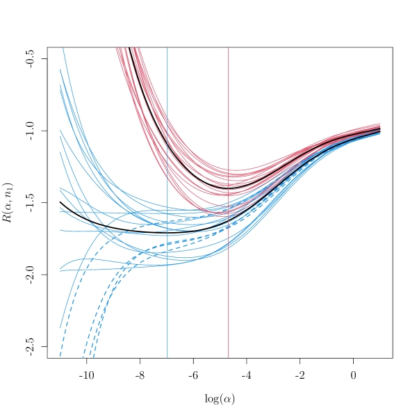
Figure 1: Estimated risk functions $\hat{R}(\alpha,n)$ in blue and $\hat{R}(\alpha,n_{1})$ in red, with $n_{1}=\sqrt{n}$, using Target Density 7, 10% measurement error, and a sample of size $n=500$. Twenty realizations are pictured, and the true criteria $R(\alpha,n)$ and $R(\alpha,n_{1})$ are pictured in black. Several catastrophically poor realizations of $\hat{R}(\alpha,n)$ are highlighted with a dashed line. The minima of $R(\alpha,n)$ and $R(\alpha,n_{1})$ are marked with a vertical line in blue and red, respectively.

We will refer to the penalty choice described in Section 1.1 as the small-$n$ risk method, and the penalty choice minimizing the criterion described in Section 2.3 as the cross-validation method. We will take $n_{1}=\sqrt{n}$ in the small-$n$ risk method throughout the paper.

Unfortunately, the simple cross-validation method performs quite poorly in practice. In Figure 1, we show in blue twenty realizations of $\hat{R}(\alpha,n)$ in one of our simulation settings. The estimates are quite wiggly in the region around the minimum, so that $\operatorname*{arg\,min}_{\alpha}\hat{R}(\alpha,n)$ is extremely variable. Some of the realizations are catastrophically poor, shown as dashed lines in the figure; these realizations are monotonically increasing on the shown interval, and attain their minima at the boundary. The poor performance is not surprising; least-squares cross-validation with standard kernel density estimators is highly variable and shows slow rates of convergence [Park and Marron, 1990], so we might expect similar behavior for deconvolution.

On the other hand, the realizations of $\hat{R}(\alpha,\sqrt{n})$ are comparatively well-behaved, shown in red in Figure 1. These curves are not wiggly near the minimum, and the minima are tightly clustered around the optimal $\alpha^{*}_{n_{1}}$.

This improvement is not due to a pointwise improvement in variance of $\hat{R}(\alpha,n)$; for a given $\alpha$, we have $\operatorname{Var}(\hat{R}(\alpha,n))\approx\operatorname{Var}(\hat{R}(\alpha,n_{1}))$. Instead, it relates to the difficulty in estimating bias. If we write $\hat{B}(\alpha,n_{1})=\frac{n_{1}-1}{n_{1}}\int|\tilde{\varphi}_{\alpha}(t)|^{2}\tilde{H}_{n}(t)\,dt-2\int\frac{\tilde{\varphi}_{\alpha}(t)}{\overline{\tilde{g}(t)}}\tilde{H}_{n}(t)\,dt$ and $V(\alpha)=\int|\tilde{\varphi}_{\alpha}(t)|^{2}\,dt$, then $\hat{R}(\alpha,n_{1})=\hat{B}(\alpha,n_{1})+V(\alpha)/n_{1}$, and by the definition of $R(\alpha,n)$ in Equation (6) and Proposition 1(ii) & (iii), we can write the error as

$$\hat{R}(\alpha,n_{1})-R(\alpha,n_{1})=\hat{B}(\alpha,n_{1})-2\pi\int(\mathbb{E}f_{n}^{\alpha}(x)-f(x))^{2}\,dx+C+O(1/n_{1}),$$ (17)

where $C=2\pi\|f\|^{2}$ does not depend on $\alpha$; so most of the error comes from estimating the squared bias and we can think of $\hat{B}(\alpha,n_{1})$ as an estimate of the squared bias. Note that $\hat{B}(\alpha,n_{1})$ depends very weakly on $n_{1}$, which only comes in through the term $(n_{1}-1)/n_{1}$. We also have that $\operatorname{Var}(\hat{R}(\alpha,n_{1}))=\operatorname{Var}(\hat{B}(\alpha,n_{1}))$ is increasing as $\alpha\to 0$ (cf. Lemma 7 for an upper bound), so this error will be worse for smaller $\alpha$. If we choose $n_{1}\ll n$, then for any given $\alpha$, $\hat{B}(\alpha,n_{1})$ changes very little. But when we choose $n_{1}\ll n$, $V(\alpha)/n_{1}$ increases proportionally to $V(\alpha)$; since $V(\alpha)\to\infty$ as $\alpha\to 0$, taking $n_{1}$ smaller allows $V(\alpha)/n_{1}$ to swamp $B(\alpha,n_{1})$ at small $\alpha$. The result is that the minima of $R(\alpha,n_{1})$ and $\hat{R}(\alpha,n_{1})$ occur at larger $\alpha$ than the minima of $R(\alpha,n)$ and $\hat{R}(\alpha,n)$, where the risk estimator has lower variance and is more well-behaved. This effect is plotted for one realization in Figure 2.

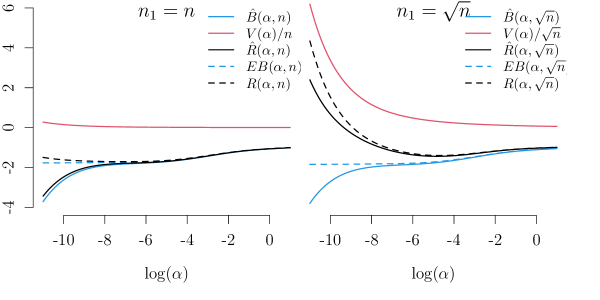
Figure 2: The estimate $\hat{R}(\alpha,n_{1})=\hat{B}(\alpha,n_{1})+V(\alpha)/n_{1}$, its component parts, and the related expectations, as described in Section 3.

4 Simulations

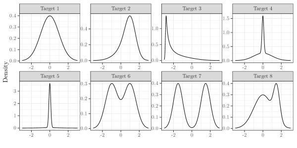
Figure 3: Target densities used in Section 4; densities 1-8 from Marron and Wand [1992].

In simulations, we explore the finite-sample performance of the cross-validation and small-$n$ risk methods on a variety of densities, and compare this to the SURE method of Yang et al. [2020] using their QP deconvolution estimator, which is closely related to the SPeD estimator here. We do the simulations under a sample size of $n=100,500$, and $1\,000$, and $p=\operatorname{Var}(E)/\operatorname{Var}(Y)=0.1$ and $0.3$. Each simulation setting is repeated $n_{\text{sim}}=1\,000$ times. We use the first eight densities from Marron and Wand [1992], setting aside the more esoteric examples like the “asymmetric double claw” density, which would present an extremely difficult problem for deconvolution. The target densities that we use are pictured in Figure 3.

In Figures 6 & 7, we show the average value of $\mathcal{L}(\hat{\alpha}_{n})/\mathcal{L}(\alpha^{*}_{n})$ with one standard error. For a very good penalty selection method, this value will be close to one. As expected from the observations in Section 3, the cross-validation choice is quite poor, the worst by far for all but one target density. The small-$n$ risk method, on the other hand, performs much better. It outperforms the SURE method in all settings except Figure 6, Target 4, and Figure 7, Targets 5 & 7, and even there the difference is not large.

Figures 4 & 5, along with Tables 1 & 2, show the real advantage of the small-$n$ risk method. Examining the figures, one sees that the SURE method often chooses a penalty that is far too small, and which yields an error larger than the oracle choice a huge amount; sometimes by a factor of 100 or more. This defect was observed by Yang et al. [2020] when they introduced this criterion. The cross-validation choice has this same problem even more strongly.

On the other hand, the small-$n$ risk method rarely chooses a parameter too small, and almost never catastrophically so. The small-$n$ risk method sometimes mildly oversmooths, which is typically less objectionable in practice.

One approach to get a handle on these features is to consider how often a method produces a catastrophic failure. Say that a catastrophic error has occured if $\mathcal{L}(\hat{\alpha}_{n})/\mathcal{L}(\alpha^{*}_{n})>10$; that is, the method incurs an error more than ten times worse than the error with the oracle smoothing parameter. Then, we study $\mathbb{P}(\mathcal{L}(\hat{\alpha}_{n})/\mathcal{L}(\alpha^{*}_{n})>10)$ under the different methods. In Table 1, we show these estimated probabilities. In 10 of the 24 settings in Table 1, the SURE method had a 5% or larger probability of catastrophic failure. On the other hand, for the small-$n$ risk method, the worst probability of catastrophic error was 1.2%, which occurred in one setting. In 19 of the 24 settings, the small-$n$ risk method’s probability of catastrophic failure was 0.1% or less.

The flip side of this question is to examine quantiles of $\mathcal{L}(\hat{\alpha}_{n})/\mathcal{L}(\alpha^{*}_{n})$. From this point of view, we see how badly things may have gone wrong in the case that our method gives us an exceptionally bad choice of parameter. In Table 2, we show the $0.99$ quantile of $\mathcal{L}(\hat{\alpha}_{n})/\mathcal{L}(\alpha^{*}_{n})$ for the three methods. For the SURE method, this quantile is over 100 in four of the 24 settings, and over 10 in 16 of them. For the small-$n$ risk method, the largest value of the quantile is 10.3, in one setting, and it is less than five in 20 of the 24 settings.

In Tables 3 & 4, we show the estimated ratio of the MISE for the SDeD with small-$n$ risk criterion choice of penalty parameter to the estimated MISE under four other settings: SPeD with oracle choice, DKDE with plug-in choice, SPeD with SURE choice, and SPeD with cross-validation. The small-$n$ risk choice performs admirably from this point of view as well. It achieved the best MISE of the four data-based methods in 20 of the 48 total settings, while the SURE was best in 15 of the 48, DKDE was best in 12 of the 48, and cross-validation was best in 1.

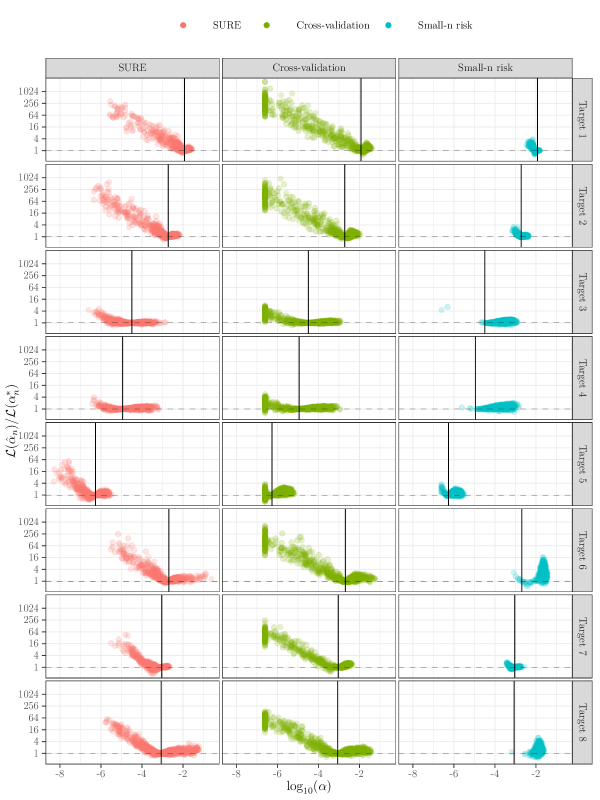
Figure 4: Outcomes of the individual simulations described in Section 3 for $n=500$, $p=10\%$ measurement error. Each point is the value of $\mathcal{L}(\hat{\alpha}_{n})/\mathcal{L}(\alpha^{*}_{n})$. Vertical lines are drawn at the MISE-optimal value of the tuning parameter.

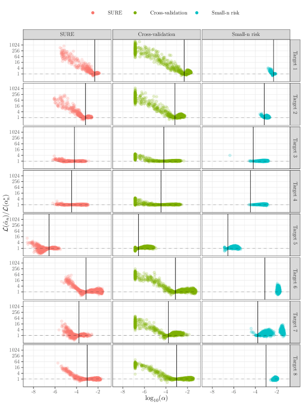
Figure 5: Outcomes of the individual simulations described in Section 3 for $n=1000$, $p=30\%$ measurement error. Each point is the value of $\mathcal{L}(\hat{\alpha}_{n})/\mathcal{L}(\alpha^{*}_{n})$. Vertical lines are drawn at the MISE-optimal value of the tuning parameter.

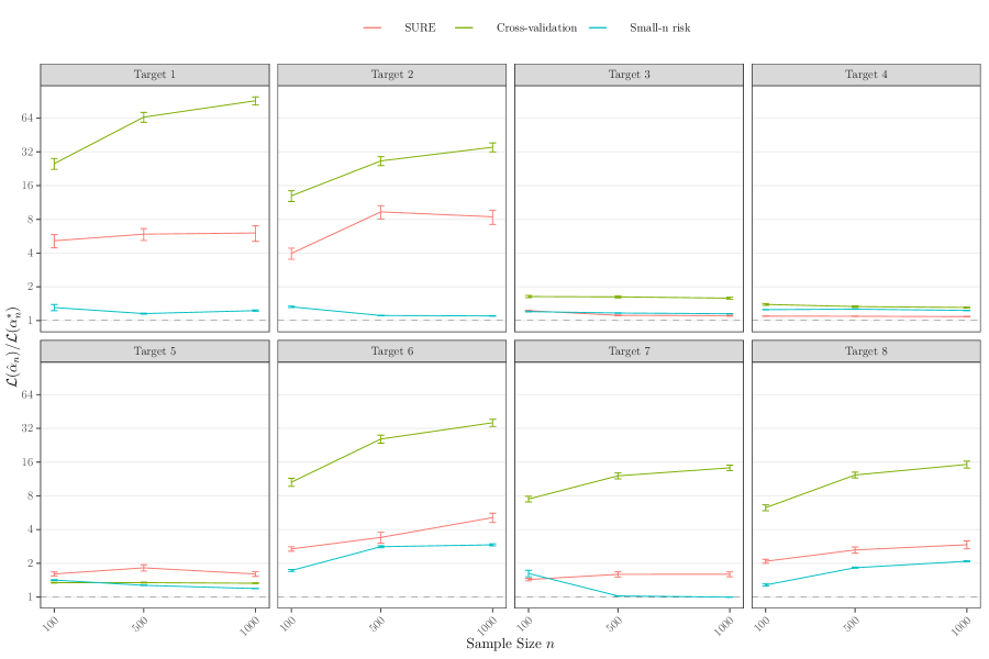
Figure 6: From simulations described in Section 3, for $p=10\%$ measurement error. For each simulation setting, we plot the average ratio of the loss with the data-based penalty to the loss with the MISE-optimal penalty parameter, with one SE error bars. An optimal method has $\mathcal{L}(\hat{\alpha}_{n})/\mathcal{L}(\alpha^{*}_{n})\to 1$ as $n\to\infty$. Note the log-scaled vertical axis.

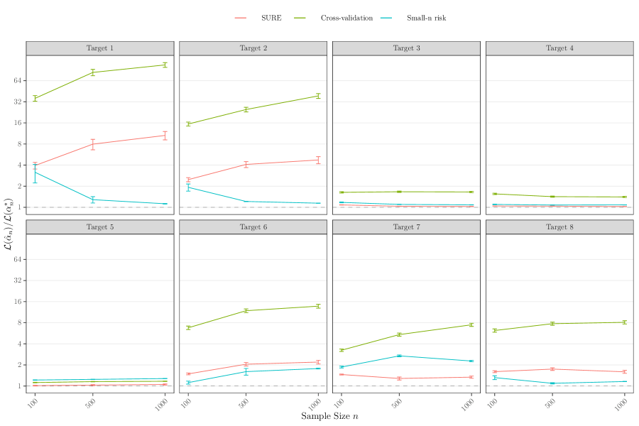
Figure 7: From simulations described in Section 3, for $p=30\%$ measurement error. For each simulation setting, we plot the average ratio of the loss with the data-based penalty to the loss with the MISE-optimal penalty parameter, with one SE error bars. An optimal method has $\mathcal{L}(\hat{\alpha}_{n})/\mathcal{L}(\alpha^{*}_{n})\to 1$ as $n\to\infty$. Note the log-scaled vertical axis.

Density	n	SURE	Cross-validation	Small-n risk
1	100	6.3	20.4	0.1
1	500	7.4	28.8	0.0
1	1000	6.3	29.6	0.0
2	100	7.1	16.9	0.1
2	500	10.8	20.4	0.0
2	1000	9.5	23.3	0.0
3	100	0.0	0.0	0.0
3	500	0.0	0.0	0.0
3	1000	0.0	0.0	0.0
4	100	0.0	0.0	0.0
4	500	0.0	0.0	0.0
4	1000	0.0	0.0	0.0
5	100	1.0	0.0	0.0
5	500	2.0	0.0	0.0
5	1000	1.1	0.0	0.0
6	100	4.0	18.3	0.3
6	500	5.3	24.9	1.2
6	1000	8.2	26.6	0.8
7	100	0.4	21.7	0.4
7	500	1.4	24.4	0.0
7	1000	1.8	26.1	0.0
8	100	2.5	17.0	0.2
8	500	5.0	23.6	0.0
8	1000	6.0	22.0	0.0

Table 1: Probability of catastrophic failure, defined as $\mathcal{L}(\hat{\alpha}_{n})/\mathcal{L}(\alpha^{*}_{n})>10$, for the three methods and settings listed, all at 10% measurement error. Based on $n_{\text{sim}}=1\,000$ simulations in each setting, described in Section 4

Density	n	SURE	Cross-validation	Small-n risk
1	100	88.8	405.9	2.8
1	500	127.4	802.6	2.6
1	1000	199.2	1159.6	3.0
2	100	56.6	223.7	3.0
2	500	191.3	357.7	2.0
2	1000	162.6	514.1	2.3
3	100	2.3	6.5	1.6
3	500	2.7	6.0	1.5
3	1000	2.6	5.3	1.4
4	100	1.7	4.7	1.8
4	500	1.6	3.9	1.8
4	1000	2.0	3.5	1.7
5	100	9.8	2.4	2.6
5	500	20.2	2.5	2.1
5	1000	12.7	2.3	1.7
6	100	19.6	125.4	5.6
6	500	45.8	354.2	10.3
6	1000	83.9	385.8	9.4
7	100	5.4	62.3	5.1
7	500	13.1	101.0	1.4
7	1000	17.4	99.4	1.2
8	100	13.9	53.5	2.1
8	500	31.1	98.7	4.1
8	1000	36.6	147.7	4.8

Table 2: $0.99$ quantile of $\mathcal{L}(\hat{\alpha}_{n})/\mathcal{L}(\alpha^{*}_{n})$ for the three methods and the settings listed, all at $10\%$ measurement error. Based on $n_{\text{sim}}=1\,000$ simulations in each setting, described in Section 4

Density	n	Optimal	DKDE	SURE	Cross-validation
1	100	1.23	0.77	0.43	0.10
1	500	1.10	0.58	0.25	0.03
1	1000	1.12	0.54	0.25	0.02
2	100	1.25	0.89	0.48	0.17
2	500	1.09	0.63	0.21	0.07
2	1000	1.07	0.54	0.18	0.04
3	100	1.18	1.04	0.97	0.73
3	500	1.15	0.96	1.04	0.71
3	1000	1.14	0.91	1.04	0.71
4	100	1.23	1.10	1.12	0.87
4	500	1.24	1.02	1.14	0.93
4	1000	1.20	0.98	1.12	0.92
5	100	1.32	0.73	0.94	1.00
5	500	1.21	0.47	0.86	0.93
5	1000	1.15	0.37	0.82	0.88
6	100	1.35	1.26	0.64	0.18
6	500	2.07	1.48	0.85	0.12
6	1000	2.23	1.32	0.59	0.09
7	100	1.59	0.93	1.15	0.26
7	500	1.03	0.45	0.69	0.10
7	1000	1.01	0.39	0.66	0.08
8	100	1.18	1.14	0.64	0.22
8	500	1.57	1.33	0.69	0.16
8	1000	1.77	1.34	0.75	0.15

Table 3: With $10\%$ measurement error, the ratio of the $\operatorname{MISE}$ of the SPeD with small-$n$ risk criterion choice of penalty parameter to the $\operatorname{MISE}$ of SPeD with oracle choice, DKDE with plug-in penalty choice, SPeD with SURE choice, and SPeD with cross-validation choice, respectively. If the value is smaller than $1$, then SPeD with small-$n$ risk choice has smaller $\operatorname{MISE}$.

Density	n	Optimal	DKDE	SURE	Cross-validation
1	100	1.90	0.84	0.73	0.12
1	500	1.24	0.40	0.25	0.03
1	1000	1.08	0.30	0.15	0.02
2	100	1.59	0.89	0.84	0.16
2	500	1.14	0.50	0.38	0.07
2	1000	1.10	0.41	0.31	0.05
3	100	1.17	1.08	1.08	0.71
3	500	1.09	0.97	1.05	0.65
3	1000	1.08	0.94	1.05	0.65
4	100	1.10	1.06	1.05	0.70
4	500	1.07	1.01	1.03	0.75
4	1000	1.08	1.00	1.05	0.76
5	100	1.21	0.83	1.16	1.03
5	500	1.20	0.69	1.14	1.02
5	1000	1.22	0.62	1.14	1.03
6	100	1.12	0.90	0.75	0.17
6	500	1.30	1.09	0.78	0.14
6	1000	1.43	1.08	0.77	0.13
7	100	1.55	1.33	1.16	0.56
7	500	2.21	1.26	1.94	0.54
7	1000	2.01	0.94	1.66	0.37
8	100	1.31	0.99	0.81	0.22
8	500	1.07	0.94	0.65	0.15
8	1000	1.11	0.95	0.74	0.15

Table 4: With $30\%$ measurement error, the ratio of the $\operatorname{MISE}$ of the SPeD with small-$n$ risk criterion choice of penalty parameter to the $\operatorname{MISE}$ of SPeD with oracle choice, DKDE with plug-in penalty choice, SPeD with SURE choice, and SPeD with cross-validation choice, respectively. If the value is smaller than $1$, then SPeD with small-$n$ risk choice has smaller $\operatorname{MISE}$.

5 Proofs

Proof of Proposition 1.

The mean integrated squared error (MISE) or risk of $f_{n}^{\alpha}$ is given by

$$\mathcal{R}(\alpha,n)=\mathbb{E}\int(f_{n}^{\alpha}(x)-f(x))^{2}\,dx=\int\operatorname{Bias}(x,\alpha)^{2}+\operatorname{Var}(f_{n}^{\alpha}(x))\,dx,$$

where $\operatorname{Bias}(x,\alpha)=\mathbb{E}f_{n}^{\alpha}(x)-f(x)$. The expectation and variance here are of course with respect to the distribution of the $Y_{j}$. It is not hard to see that $\mathbb{E}[f_{n}^{\alpha}(x)]=\mathbb{E}[\varphi_{\alpha}(x-Y_{1})]=\varphi_{\alpha}*g*f(x)$. Then the Plancherel Theorem yields that

$$\int\operatorname{Bias}(x,\alpha)^{2}\,dx=\int\left(\varphi_{\alpha}*g*f(x)-f(x)\right)^{2}\,dx=\frac{1}{2\pi}\int|\tilde{\varphi}_{\alpha}(t)\tilde{g}(t)-1|^{2}|\tilde{f}(t)|^{2}\,dt.$$

Now, $\operatorname{Var}(f_{n}^{\alpha}(x))=\frac{1}{n}\operatorname{Var}(\varphi_{\alpha}(x-Y))$, and

$$\int\operatorname{Var}(\varphi_{\alpha}(x-Y))\,dx =\int\mathbb{E}[\varphi_{\alpha}(x-Y)^{2}]-\mathbb{E}[\varphi_{\alpha}(x-Y)]^{2}\,dx$$

$$=\int\int[\varphi_{\alpha}(x-y)]^{2}[g*f(y)]\,dy\,dx-\int[\varphi_{\alpha}*g*f(x)]^{2}\,dx$$

$$=\int\left(\int[\varphi_{\alpha}(x-y)]^{2}\,dx\right)[g*f(y)]\,dy-\int[\varphi_{\alpha}*g*f(x)]^{2}\,dx$$

$$=\int\left(\int[\varphi_{\alpha}(x)]^{2}\,dx\right)[g*f(y)]\,dy-\int[\varphi_{\alpha}*g*f(x)]^{2}\,dx$$

$$=\int[\varphi_{\alpha}(x)]^{2}\,dx-\int[\varphi_{\alpha}*g*f(x)]^{2}\,dx$$

$$=\frac{1}{2\pi}\int|\tilde{\varphi}_{\alpha}(t)|^{2}\,dt-\frac{1}{2\pi}\int|\tilde{\varphi}_{\alpha}(t)\tilde{g}(t)\tilde{f}(t)|^{2}\,dx.$$

Combining the above yields the first three equations of Proposition 1. The final equation follows from simplifying $2\pi(\mathcal{R}(\alpha,n)-\|f\|^{2})$. Note that $\tilde{\varphi}_{\alpha}(t)\tilde{g}(t)=\frac{|\tilde{g}(t)|^{2}}{|\tilde{g}(t)|^{2}+\alpha|t|^{2m}}$ is real, so $\Re(\tilde{\varphi}_{\alpha}(t)\tilde{g}(t))=\tilde{\varphi}_{\alpha}(t)\tilde{g}(t)$. We will write the integrals in brief form to save space.

$$2\pi(\mathcal{R} (\alpha,n)-\|f\|^{2})$$ (18)

$$=2\pi\left[\frac{1}{2\pi}\int|\tilde{\varphi}_{\alpha}\tilde{g}-1|^{2}|\tilde{f}|^{2}+\frac{1}{2\pi n}\int|\tilde{\varphi}_{\alpha}|^{2}-\frac{1}{2\pi n}\int|\tilde{\varphi}_{\alpha}\tilde{g}\tilde{f}|^{2}-\|f\|^{2}\right]$$

$$=\int|\tilde{\varphi}_{\alpha}\tilde{g}\tilde{f}|^{2}-2\int\tilde{\varphi}_{\alpha}\tilde{g}|\tilde{f}|^{2}+2\pi\|f\|^{2}+\frac{1}{n}\int|\tilde{\varphi}_{\alpha}|^{2}-\frac{1}{n}\int|\tilde{\varphi}_{\alpha}\tilde{g}\tilde{f}|^{2}-2\pi\|f\|^{2}$$

$$=\frac{n-1}{n}\int|\tilde{\varphi}_{\alpha}\tilde{g}\tilde{f}|^{2}-2\int\tilde{\varphi}_{\alpha}\tilde{g}\frac{|\tilde{g}|^{2}}{\tilde{g}\overline{\tilde{g}}}|\tilde{f}|^{2}+\frac{1}{n}\int|\tilde{\varphi}_{\alpha}|^{2}$$

$$=\frac{n-1}{n}\int|\tilde{\varphi}_{\alpha}\tilde{g}\tilde{f}|^{2}-2\int\frac{\tilde{\varphi}_{\alpha}}{\overline{\tilde{g}}}|\tilde{g}\tilde{f}|^{2}+\frac{1}{n}\int|\tilde{\varphi}_{\alpha}|^{2}$$

The result follows from $\tilde{h}=\tilde{g}\tilde{f}$. ∎

Proof of Proposition 2.

Let $f^{\alpha}(x)=\varphi_{\alpha}*h(x)$, just as in Kent and Ruppert [2023]. Note that with the simplified estimator here, we have $\mathbb{E}f_{n}^{\alpha}(x)=f^{\alpha}(x)$. Lemma 5 of Kent and Ruppert [2023] gives upper bounds for $\int(f^{\alpha}(x)-f(x))^{2}\,dx$, which in the present case is exactly the integrated squared bias. By Proposition 1 and Lemma 8 here and Lemma 5(i) of Kent and Ruppert [2023],

$$\mathcal{R}(\alpha,n) =\int(f^{\alpha}(x)-f(x))^{2}\,dx+\int\operatorname{Var}(f_{n}^{\alpha}(x))\,dx$$ (19)

$$\leq C_{1}[m\log(m^{-1}\alpha^{-\frac{1}{m}})]^{-k}+\frac{C_{2}}{n\alpha}.$$

The second term becomes $\frac{C_{2}}{n\alpha}=C_{3}[\log n]^{-k}$. For the second term, with asymptotic order as $\alpha\to 0$ or $n\to\infty$,

$$\frac{1}{m\log(m^{-1}\alpha^{-\frac{1}{m}})} \asymp\frac{1}{\log\alpha^{-1}}$$ (20)

$$=\frac{1}{\log(n[\log n^{k}]^{-k})}$$

$$=\frac{1}{\log n-k\log k-k\log\log n}$$

$$\sim\frac{1}{\log n},$$

so $[m\log(m^{-1}\alpha^{-\frac{1}{m}})]^{-k}\asymp[\log n]^{-k}$. Combining these two yields that $\mathcal{R}(\alpha_{n},n)=O([\log n]^{-k})$. ∎

Proof of Lemma 3.

Doing a little algebra gives us

$$|\tilde{P}_{n}(t)|^{2} =\left[\frac{1}{n}\sum_{j=1}^{n}e^{-itY_{j}}\right]\left[\frac{1}{n}\sum_{j=1}^{n}\overline{e^{-itY_{j}}}\right]$$

$$=\frac{1}{n^{2}}\sum_{j=1}^{n}\sum_{k=1}^{n}e^{-itY_{j}}\overline{e^{-itY_{k}}}$$

$$=\frac{1}{n^{2}}\sum_{j=1}^{n}\sum_{k=1}^{n}e^{-it(Y_{j}-Y_{k})},$$

so $\mathbb{E}[|\tilde{P}_{n}(t)|^{2}]=\frac{1}{n^{2}}\sum_{j=1}^{n}\sum_{k=1}^{n}\mathbb{E}[e^{-it(Y_{j}-Y_{k})}]$. If $j=k$, then $\mathbb{E}[e^{-it(Y_{j}-Y_{k})}]=1$. If $j\neq k$, then $\mathbb{E}[e^{-it(Y_{j}-Y_{k})}]=\tilde{h}(t)\tilde{h}(-t)=|\tilde{h}(t)|^{2}$, since it is the Fourier transform of $Y_{1}-Y_{2}$. Noting that there are $n$ summands with $j=k$ and $n(n-1)$ with $j\neq k$ yields the result. ∎

Proof of Lemma 4.

First, let’s express $\hat{R}(\alpha,n_{1})$ as a U-statistic, writing the integrals in brief form to save space.

$$\hat{R}(\alpha,n_{1}) =C_{1}+\frac{n_{1}-1}{n_{1}}\int|\tilde{\varphi}_{\alpha}|^{2}\tilde{H}_{n}-2\int\frac{\tilde{\varphi}_{\alpha}}{\overline{\tilde{g}}}\tilde{H}_{n}$$ (21)

$$=C_{1}+\frac{n_{1}-1}{n_{1}}\int|\tilde{\varphi}_{\alpha}|^{2}\frac{n}{n-1}\left(|\tilde{P}_{n}|^{2}-\frac{1}{n}\right)-2\int\frac{\tilde{\varphi}_{\alpha}}{\overline{\tilde{g}}}\frac{n}{n-1}\left(|\tilde{P}_{n}|^{2}-\frac{1}{n}\right)$$

$$=C_{2}+\int\left(\frac{(n_{1}-1)n}{n_{1}(n-1)}|\tilde{\varphi}_{\alpha}|^{2}-\frac{2n}{n-1}\frac{\tilde{\varphi}_{\alpha}}{\overline{\tilde{g}}}\right)|\tilde{P}_{n}|^{2}$$

Now, let $\tilde{\theta}_{\alpha}(t)=\frac{n(n_{1}-1)}{n_{1}(n-1)}|\tilde{\varphi}_{\alpha}(t)|^{2}-\frac{2n}{n-1}\frac{\tilde{\varphi}_{\alpha}(t)}{\overline{\tilde{g}(t)}}$ and $\theta_{\alpha}$ is its inverse Fourier transform. One can check the definition of $\tilde{\varphi}_{\alpha}$ to see that $\tilde{\theta}_{\alpha}(t)$ is purely real, symmetric, and integrable, so $\theta_{\alpha}(x)$ exists and is real and symmetric. Then we have

$$\hat{R}(\alpha,n_{1}) =C_{2}+\int\tilde{\theta}_{\alpha}(t)|\tilde{P}_{n}(t)|^{2}\,dt$$ (22)

$$=C_{2}+\frac{1}{n^{2}}\sum_{j=1}^{n}\sum_{k=1}^{n}\theta_{\alpha}(Y_{j}-Y_{k})$$

$$=C_{2}+\frac{1}{n}\theta_{\alpha}(0)+\frac{2}{n(n-1)}\sum_{1\leq j<k\leq n}\theta_{\alpha}(Y_{j}-Y_{k})$$

$$=C_{3}+\frac{1}{\binom{n}{2}}\sum_{1\leq j<k\leq n}\theta_{\alpha}(Y_{j}-Y_{k}).$$

Now, for the bounds. We begin with $|\theta^{\prime}_{\alpha}(x)|=\left|\frac{1}{2\pi}\int e^{itx}it\tilde{\theta}_{\alpha}(t)\,dt\right|\leq\frac{1}{2\pi}\int|t|\cdot|\tilde{\theta}_{\alpha}(t)|\,dt$. Now, we can write $|\tilde{\theta}_{\alpha}(t)|$ in the following way.

$$|\tilde{\theta}_{\alpha}(t)| =\left|\frac{n(n_{1}-1)}{n_{1}(n-1)}|\tilde{\varphi}_{\alpha}(t)|^{2}-\frac{2n}{n-1}\frac{\tilde{\varphi}_{\alpha}(t)}{\overline{\tilde{g}(t)}}\right|$$ (23)

$$=\left|\frac{n}{n-1}\left(\frac{\frac{n_{1}-1}{n_{1}}|\tilde{g}(t)|^{2}}{(|\tilde{g}(t)|^{2}+\alpha|t|^{2m})^{2}}-\frac{2(|\tilde{g}(t)|^{2}+\alpha|t|^{2m})}{(|\tilde{g}(t)|^{2}+\alpha|t|^{2m})^{2}}\right)\right|$$

$$=\left|-\frac{n}{n-1}\left(\frac{\frac{n_{1}+1}{n_{1}}|\tilde{g}(t)|^{2}+\alpha|t|^{2m}}{(|\tilde{g}(t)|^{2}+\alpha|t|^{2m})^{2}}\right)\right|$$

$$=\frac{n}{n-1}\left(\frac{\frac{n_{1}+1}{n_{1}}|\tilde{g}(t)|^{2}+\alpha|t|^{2m}}{(|\tilde{g}(t)|^{2}+\alpha|t|^{2m})^{2}}\right),$$

so

$$|\theta^{\prime}_{\alpha}(x)|\leq\frac{n(n_{1}+1)}{2\pi(n-1)n_{1}}\int\frac{|t|\cdot|\tilde{g}(t)|^{2}}{(|\tilde{g}(t)|^{2}+\alpha|t|^{2m})^{2}}\,dt+\frac{n}{2\pi(n-1)}\int\frac{\alpha|t|^{2m+1}}{(|\tilde{g}(t)|^{2}+\alpha|t|^{2m})^{2}}\,dt$$ (24)

For the first integral in Equation (24), we have, choosing ${\varepsilon}>0$ small enough that $|\tilde{g}(t)|>c>0$ for all $0\leq t\leq{\varepsilon}$, i.e. $|\tilde{g}(t)|$ is bounded away from zero:

$$\int\frac{|t|\cdot|\tilde{g}(t)|^{2}}{(|\tilde{g}(t)|^{2}+\alpha|t|^{2m})^{2}}\,dt =2\int_{0}^{\varepsilon}\frac{|t|\cdot|\tilde{g}(t)|^{2}}{(|\tilde{g}(t)|^{2}+\alpha|t|^{2m})^{2}}\,dt+2\int_{\varepsilon}^{\infty}\frac{|t|\cdot|\tilde{g}(t)|^{2}}{(|\tilde{g}(t)|^{2}+\alpha|t|^{2m})^{2}}\,dt$$ (25)

$$\leq 2\int_{0}^{\varepsilon}|t|\cdot|\tilde{g}(t)|^{-2}\,dt+2\int_{\varepsilon}^{\infty}\frac{|t|\cdot|\tilde{g}(t)|^{2}}{(2\sqrt{\alpha}|\tilde{g}(t)|\cdot|t|^{m})^{2}}\,dt$$

$$\leq 2\int_{0}^{\varepsilon}|t|\cdot|\tilde{g}(t)|^{-2}\,dt+\frac{1}{2\alpha}\int_{\varepsilon}^{\infty}|t|^{1-2m}\,dt$$

$$=C_{\varepsilon}+\frac{2C^{\prime}_{\varepsilon}}{\alpha}\leq\frac{C_{\varepsilon,M}}{\alpha}$$

Now, for the second integral in Equation (24), with the same choice of $\varepsilon$,

$$\int\frac{\alpha|t|^{2m+1}}{(|\tilde{g}(t)|^{2}+\alpha|t|^{2m})^{2}}\,dt =2\int_{0}^{\varepsilon}\frac{\alpha|t|^{2m+1}}{(|\tilde{g}(t)|^{2}+\alpha|t|^{2m})^{2}}\,dt+2\int_{\varepsilon}^{\infty}\frac{\alpha|t|^{2m+1}}{(|\tilde{g}(t)|^{2}+\alpha|t|^{2m})^{2}}\,dt$$ (26)

$$=2M\int_{0}^{\varepsilon}|t|^{2m+1}\cdot|\tilde{g}(t)|^{-4}\,dt+\frac{2}{\alpha}\int_{\varepsilon}^{\infty}|t|^{1-2m}\,dt$$

$$\leq\frac{C^{\prime}_{\varepsilon,M}}{\alpha}.$$

Combining these with Equation (24) and the fact that for $n,n_{1}>1$, $(n_{1}+1)/n_{1}\leq 1.5$ and $n/(n-1)\leq 2$, we find

$$|\theta^{\prime}_{\alpha}(x)|\leq\frac{C^{\prime}}{\alpha}.$$ (27)

Since this holds for any $x$, it holds uniformly.

To bound $|\theta_{\alpha}(x)|$, we begin with $|\theta_{\alpha}(x)|=\left|\frac{1}{2\pi}\int e^{itx}\tilde{\theta}_{\alpha}(t)\,dt\right|\leq\frac{1}{2\pi}\int|\tilde{\theta}_{\alpha}(t)|\,dt$ From here, the argument is identical to the one just made for $|\theta^{\prime}_{\alpha}(x)|$, and just yields different constants. ∎

Proof of Proposition 5.

We use McDiarmid’s inequality. By the bound in Lemma 4, we have that $|\theta_{\alpha}(x)-\theta_{\alpha}(y)|\leq C/\alpha$. Use the U-statistic representation of $\hat{R}(\alpha,n_{1})$ to find

$$|\hat{R}(\alpha,n_{1};Y_{1},\dots,Y_{i},\dots,Y_{n})- \hat{R}(\alpha,n_{1};Y_{1},\dots,Y_{i}^{\prime},\dots,Y_{n})|$$ (28)

$$\leq\left|\frac{2}{n(n-1)}\sum_{j\neq i}\theta_{\alpha}(Y_{j}-Y_{i})-\theta_{\alpha}(Y_{j}-Y_{i}^{\prime})\right|$$

$$\leq\frac{2}{n(n-1)}\sum_{j\neq i}|\theta_{\alpha}(Y_{j}-Y_{i})-\theta_{\alpha}(Y_{j}-Y_{i}^{\prime})|$$

$$\leq\frac{2}{n(n-1)}\cdot(n-1)\cdot\frac{C}{\alpha}$$

$$=\frac{C}{n\alpha}.$$

Thus we have the coordinatewise bounds $c_{i}=\frac{C}{n\alpha}$ so that $\sum_{i=1}^{n}c_{i}^{2}=\frac{C^{2}}{n\alpha^{2}}$. Applying McDiarmid’s inequality gives

$$\mathbb{P}(r_{n_{1}}^{-1}|\hat{R}(\alpha,n_{1})-R(\alpha,n_{1})|>\varepsilon)\leq 2\exp\{-2C_{1}\varepsilon^{2}r_{n_{1}}^{2}n\alpha^{2}\}\leq 2\exp\{-2C_{2}\varepsilon^{2}(r_{n_{1}}b_{n_{1}})^{2}n\}$$ (29)

A union bound gives the stated result. ∎

Proof of Lemma 7.

First, we find the upper bound $\operatorname{Var}(\hat{R}(\alpha,n_{1}))\leq\frac{2}{n}\operatorname{Var}(\theta_{\alpha}(Y_{j}-Y_{k}))$ using a result on U-statistics. Then, by Lemma 4, $\theta_{\alpha}(\cdot)$ is Lipschitz with constant $C_{\alpha}\leq\frac{C^{\prime}}{\alpha}$, so we can bound this variance by $\operatorname{Var}(\theta_{\alpha}(Y_{j}-Y_{k}))\leq C_{\alpha}^{2}\operatorname{Var}(Y_{j}-Y_{k})\leq\frac{C^{\prime 2}2\sigma^{2}}{\alpha^{2}}$. Combining these gives the desired conclusion.

Now the variance of $\hat{R}(\alpha,n_{1})$ is exactly the variance of the U-statistic with kernel $\theta_{\alpha}(Y_{j}~{}-~{}Y_{k})$ given in Lemma 4. By [Lee, 1990, Chapter 1.3, Theorem 3], we have

$$\operatorname{Var}(\hat{R}(\alpha,n_{1}))=\frac{1}{\binom{n}{2}}(2(n-2)\sigma_{1}^{2}+\sigma_{2}^{2}),$$ (30)

where $\sigma_{1}^{2}=\operatorname{Var}(\mathbb{E}[\theta_{\alpha}(Y_{j}-Y_{k})|Y_{j}])$ and $\sigma_{2}^{2}=\operatorname{Var}(\theta_{\alpha}(Y_{j}-Y_{k}))$. By [Lee, 1990, Chapter 1.3, Theorem 4], $2\sigma_{1}^{2}\leq\sigma_{2}^{2}$, so

$$\operatorname{Var}(\hat{R}(\alpha,n_{1}))\leq\frac{1}{\binom{n}{2}}((n-2)\sigma_{2}^{2}+\sigma_{2}^{2})=\frac{2\sigma_{2}^{2}}{n}.$$ (31)

The variance of $Y_{j}-Y_{k}$ is $2\operatorname{Var}(Y_{1})$ since $Y_{j}$ and $Y_{k}$ are independent. If $\theta_{\alpha}(\cdot)$ is Lipschitz with constant $C_{\alpha}$, then

$$\operatorname{Var}(\hat{R}(\alpha,n_{1}))\leq\frac{2\operatorname{Var}(\theta_{\alpha}(Y_{j}-Y_{k}))}{n}\leq\frac{4C_{\alpha}^{2}}{n}\operatorname{Var}(Y_{1})$$ (32)

The fact that $C_{\alpha}\leq\frac{C^{\prime}}{\alpha}$ gives the result. ∎

Lemma 8.

If $m\geq 1$, then for $0<\alpha<M$, $\int|\tilde{\varphi}_{\alpha}(t)|^{2}\,dt\leq\frac{C}{\alpha}$. As a consequence, $\int\operatorname{Var}(f_{n}^{\alpha}(x))\,dx\leq\frac{C^{\prime}}{n\alpha}$. The constants $C$ and $C^{\prime}$ depend on $g$, $m$, and $M$.

Proof of Lemma 8.

By dropping $\alpha|t|^{2m}$ in the denominator, it can be seen that $|\tilde{\varphi}_{\alpha}(t)|\leq|\tilde{g}(t)|^{-1}$. Applying the inequality $a+b\geq 2\sqrt{ab}$ to the denominator yields $|\tilde{\varphi}_{\alpha}(t)|\leq\frac{1}{2}\alpha^{-\frac{1}{2}}|t|^{-m}$. Then $\int|\tilde{\varphi}_{\alpha}(t)|^{2}\,dt\leq\frac{1}{\alpha}\int\min\{M|\tilde{g}(t)|^{-2},\frac{1}{4}|t|^{-2m}\}\,dt$. The integral is finite because $|\tilde{g}(t)|^{-2}$ is integrable near zero, while $|t|^{-2m}$ is integrable away from zero. The variance bound then follows immediately from the expression for the variance in Proposition 1. ∎

References

- Delaigle and Gijbels [2004a] A. Delaigle and I. Gijbels. Bootstrap bandwidth selection in kernel density estimation from a contaminated sample. Annals of the Institute of Statistical Mathematics, 56(1):19–47, March 2004a. doi: 10.1007/BF02530523.
- Delaigle and Gijbels [2004b] A. Delaigle and I. Gijbels. Practical bandwidth selection in deconvolution kernel density estimation. Computational Statistics & Data Analysis, 45(2):249–267, March 2004b. doi: 10.1016/S0167-9473(02)00329-8.
- Faraway and Jhun [1990] Julian J. Faraway and Myoungshic Jhun. Bootstrap Choice of Bandwidth for Density Estimation. Journal of the American Statistical Association, 85(412):1119–1122, December 1990. doi: 10.1080/01621459.1990.10474983.
- Hall [1982] Peter Hall. Limit theorems for stochastic measures of the accuracy of density estimators. Stochastic Processes and their Applications, 13(1):11–25, July 1982. doi: 10.1016/0304-4149(82)90003-5.
- Hall [1990] Peter Hall. Using the bootstrap to estimate mean squared error and select smoothing parameter in nonparametric problems. Journal of Multivariate Analysis, 32(2):177–203, February 1990. doi: 10.1016/0047-259X(90)90080-2.
- Kent and Ruppert [2023] David Kent and David Ruppert. Smoothness-Penalized Deconvolution (SPeD) of a Density Estimate. Journal of the American Statistical Association, 0(0):1–11, 2023. doi: 10.1080/01621459.2023.2259028.
- Lee [1990] A. J. Lee. U-statistics: theory and practice. M. Dekker, New York, 1990. ISBN 978-0-8247-8253-5.
- Marron and Wand [1992] J. S. Marron and M. P. Wand. Exact Mean Integrated Squared Error. The Annals of Statistics, 20(2):712–736, June 1992. doi: 10.1214/aos/1176348653.
- Park and Marron [1990] Byeong U. Park and J. S. Marron. Comparison of Data-Driven Bandwidth Selectors. Journal of the American Statistical Association, 85(409):66–72, 1990. doi: 10.2307/2289526.
- Yang et al. [2020] Ran Yang, Daniel W. Apley, Jeremy Staum, and David Ruppert. Density Deconvolution With Additive Measurement Errors Using Quadratic Programming. Journal of Computational and Graphical Statistics, 29(3):580–591, July 2020. doi: 10.1080/10618600.2019.1704294.
- Youndjé and Wells [2008] Élie Youndjé and Martin T. Wells. Optimal bandwidth selection for multivariate kernel deconvolution density estimation. TEST, 17(1):138–162, May 2008. doi: 10.1007/s11749-006-0027-5.