Scalable network reconstruction in subquadratic time

Abstract

Network reconstruction consists in determining the unobserved pairwise couplings between $N$ nodes given only observational data on the resulting behavior that is conditioned on those couplings — typically a time-series or independent samples from a graphical model. A major obstacle to the scalability of algorithms proposed for this problem is a seemingly unavoidable quadratic complexity of $O(N^{2})$, corresponding to the requirement of each possible pairwise coupling being contemplated at least once, despite the fact that most networks of interest are sparse, with a number of non-zero couplings that is only $O(N)$. Here we present a general algorithm applicable to a broad range of reconstruction problems that achieves its result in subquadratic time, with a data-dependent complexity loosely upper bounded by $O(N^{3/2}\log N)$, but with a more typical log-linear complexity of $O(N\log^{2}N)$. Our algorithm relies on a stochastic second neighbor search that produces the best edge candidates with high probability, thus bypassing an exhaustive quadratic search. In practice, our algorithm achieves a performance that is many orders of magnitude faster than the quadratic baseline, allows for easy parallelization, and thus enables the reconstruction of networks with hundreds of thousands and even millions of nodes and edges.

I Introduction

Networks encode the pairwise interactions that determine the dynamical behavior of a broad class of interconnected systems. However, in many important cases the interactions themselves are not directly observed, and instead we have access only to their indirect outcomes, usually as samples from a multivariate distribution modeled as a probabilistic graphical model [1, 2, 3], or from time-series data representing some dynamics conditioned on the network structure [4, 5]. Instances of this problem include the inference of interactions between microbial species from co-occurrence data [6], financial market couplings from stock prices [7], protein structure from amino-acid contact maps [8], gene regulatory networks from expression data [9], neural connectivity from fMRI and EEG data [10], and epidemic contact tracing [11], among others.

Perhaps the most well studied formulation of the network reconstruction problem is covariance selection [12], where it is assumed that the data consist of independent samples of a multivariate Gaussian, and the objective is to infer its precision matrix — often assumed to be sparse. The most widely employed algorithm for this purpose is the graphical LASSO (GLASSO) [13], and its many variations [14, 15]. More generally, one can consider arbitrary probabilistic graphical models (a.k.a. Markov random fields) [16], where the latent network structure encodes the conditional dependence between variables. Covariance selection is a special case of this family where the variables are conditionally normally distributed, resulting in an analytical likelihood, unlike the general case which involves intractable normalization constants. A prominent non-Gaussian graphical model is the Ising model [17], applicable for binary variables, which has a wide range of applications.

The vast majority of algorithmic approaches so far employed to the network reconstruction problem cannot escape a complexity of at least $O(N^{2})$, where $N$ is the number of nodes in the network. The original GLASSO algorithm for covariance selection has a complexity of $O(N^{3})$. By exploiting properties that are specific to the covariance selection problem (and hence do not generalize to the broader reconstruction context), the faster QUIC [18] and BigQUIC [19] approximative methods have $O(N^{2})$ and $O(NE)$ complexities, respectively, with $E$ being the number of edges (i.e. nonzero entries in the reconstructed matrix), such that the latter also becomes quadratic in the usual sparse regime with $E=O(N)$. Likewise, for the inverse Ising model [17, 20] or graphical models in general [16, 21] no known method can improve on a $O(N^{2})$ complexity, and the same is true for reconstruction from time-series [22, 4]. To the best of our knowledge, no general approach exists to the network reconstruction problem with a lower complexity than $O(N^{2})$, unless strong assumptions on the true network structure are made. Naively, one could expect this barrier to be a fundamental one, since for the reconstruction task — at least in the general case — we would be required to probe the existence of every possible pairwise coupling at least once.

Instead, in this work we show that it is in fact possible to implement a general network reconstruction scheme that yields subquadratic complexity, without relying on the specific properties of any particular instance of the problem. Our approach is simple, and relies on a stochastic search for the best update candidates (i.e. edges that need to be added, removed, or updated) in an iterative manner that starts from a random graph and updates the candidate list by inspecting the second neighbors of this graph — an approach which leads to log-linear performance [23, 24, 25]. Furthermore, every step of our algorithm is easily parallelizable, allowing its application for problems of massive size.

This paper is organized as follows. In Sec. II we introduce the general reconstruction scenario, and the coordinate descent algorithm, which will function as our baseline with quadratic complexity. In Sec. III we describe our improvement over the baseline, and analyze its algorithmic complexity. In Sec. IV we evaluate the performance of our approach on a variety of synthetic and empirical data, and in Sec. V we showcase our algorithm with some selected large-scale empirical network reconstruction problems. We finalize in Sec. VI with a conclusion.

II General reconstruction scenario and coordinate descent (CD) baseline

We are interested in a general reconstruction setting where we assume some data $\bm{X}$ are sampled from a generative model with a likelihood

$$P(\bm{X}|\bm{W}),$$ (1)

where $\bm{W}$ is a $N\times N$ symmetric matrix corresponding to the weights of an undirected graph of $N$ nodes. In most cases of interest, the matrix $\bm{W}$ is sparse, i.e. its number of non-zero entries is $O(N)$, but otherwise we assume no special structure. Typically, the data are either a $N\times M$ matrix of $M$ independent samples, with $X_{im}$ being a value associated with node $i$ for sample $m$, such that

$$P(\bm{X}|\bm{W})=\prod_{m=1}^{M}P(\bm{x}_{m}|\bm{W}),$$ (2)

with $\bm{x}_{m}$ being the $m$-th column of $\bm{X}$, or a Markovian time series with

$$P(\bm{X}|\bm{W})=\prod_{m=1}^{M}P(\bm{x}_{m}|\bm{x}_{m-1},\bm{W}),$$ (3)

given some initial state $\bm{x}_{0}$. Our algorithm will not rely strictly on any such particular formulations, only on a generic posterior distribution

$$\pi(\bm{W})=P(\bm{W}|\bm{X})=\frac{P(\bm{X}|\bm{W})P(\bm{W})}{P(\bm{X})}$$ (4)

that needs to be computable only up to normalization. We focus on the MAP point estimate

$$\widehat{\bm{W}}=\underset{\bm{W}}{\operatorname{arg\ max}}\;\pi(\bm{W}).$$ (5)

For many important instances of this problem, such as covariance selection [12, 13] and the inverse Ising model [17] the optimization objective above is convex. In this case, one feasible approach is the coordinate descent (CD) algorithm [26], which proceeds by iterating over all variables in sequence, and solving a one-dimensional optimization (which is guaranteed to be convex as well), and stopping when a convergence threshold is reached (see Algorithm 1).

Algorithm 1 has complexity $O(\tau N^{2})$, assuming step (1) can be done in time $O(1)$ (e.g. using bisection search), where $\tau$ is the number of iterations required for convergence — which in general will depend on the particulars of the problem and initial state, but typically we have $\tau=O(1)$.

Algorithm 1 Coordinate descent (CD)

Input: Objective $\pi(\bm{W})$, initial state $\bm{W}_{0}$, convergence criterion $\epsilon$

Output: Estimate $\widehat{\bm{W}}=\underset{\bm{W}}{\operatorname{arg\ max}}\;\pi(\bm{W})$

$\bm{W}\leftarrow\bm{W}_{0}$

$\Delta\leftarrow 0$ $i<j$

$W_{ij}^{\prime}\leftarrow\operatorname{arg\ max}_{W_{ij}}\;\pi(\bm{W})$ $\triangleright$ (1)

$\Delta\leftarrow\Delta+|W_{ij}^{\prime}-W_{ij}|$

$W_{ij}\leftarrow W_{ij}^{\prime}$ $\Delta<\epsilon$

$\widehat{\bm{W}}\leftarrow\bm{W}$

Note that the CD algorithm does not require a differentiable objective $\pi(\bm{W})$, but convergence to the global optimum is only guaranteed if it is convex and sufficiently smooth [27]. In practice, CD is the method of choice for covariance selection and the inverse Ising model, with a speed of convergence that often exceeds gradient descent (which is not even strictly applicable when non-differentiable regularization is used, such as the $L_{1}$ of GLASSO [13]), since each coordinate can advance further with more independence from the remaining ones, unlike with gradient descent where all coordinates are restricted by the advance of the slowest one.

For a nonconvex objective $\pi(\bm{W})$, the CD algorithm will in general not converge to the global optimum. Nevertheless, it is a fundamental baseline that often gives good results in practice even in nonconvex instances, and can serve as a starting point for more advanced algorithms. In this work we are not primarily concerned with complications due to nonconvexity, but rather with a general approach that circumvents the need to update all ${N\choose 2}$ entries of the matrix $\bm{W}$.

Our objective is to reduce the $O(N^{2})$ complexity of the CD algorithm. But, before continuing, we will remark on the feasibility of the reconstruction problem, and the obstacle that this quadratic complexity represents. At first, one could hypothesize that the size of the data matrix $\bm{X}$ would need to be impractically large to allow for the reconstruction of networks with $N$ in the order of hundreds of thousands or millions. In such a case, a quadratic complexity would be the least of our concerns for problem sizes that are realistically feasible. However, for graphical models it is possible to show that the number of samples required for accurate reconstruction scales only with $M=O(\log N)$ [16, 28, 29, 30, 21], meaning that reconstruction of large networks with relatively little information is possible. An informal version of the argument presented in Ref. [16] that demonstrates this intuitively is as follows. Suppose we are primarily concerned with correctly recovering the graphical structure of $\bm{W}$, i.e. the binary graph $\bm{G}(\bm{W})$ with edges corresponding to the non-zero entries of $\bm{W}$, and that our prior $P(\bm{W})$ corresponds to a uniform distribution $P(\bm{G})=|\mathcal{G}_{d}|^{-1}$ on the set $\mathcal{G}_{d}$ of graphs with $N$ nodes and maximum degree $d$. If the entries of $\bm{X}$ can take values in a finite set of size $A$, then the set $\mathcal{X}$ of possible data matrices $\bm{X}$ has size $|\mathcal{X}|=A^{NM}$. Therefore, if the true graph $\bm{G}$ is sampled from $P(\bm{G})$, then a lower bound on the probability of error (i.e. $\bm{G}(\widehat{\bm{W}})\neq\bm{G}$) is given by $1-A^{NM}/|\mathcal{G}_{d}|$, obtained by observing that the set of graphs for which the MAP estimate of Eq. 5 gives the correct result has size at most $|\mathcal{X}|=A^{NM}$ (since $\widehat{\bm{W}}$ is a deterministic function of $\bm{X}$). For $d$ growing sublinearly on $N$ we have $\log|\mathcal{G}_{d}|=\Omega(dN\log N)$ [16], therefore it follows that reconstruction is possible with probability $o(1)$ as long as $M=\Omega(d\log N)$. Although this is only a lower bound on the sample complexity, it indicates that there is no obvious information theoretical requirement for it to be higher. In fact, there are a series of more detailed results that prove that the sample complexity scales indeed as $O(\log N)$ for networks with bounded degree for elementary types of graphical models [16, 31, 30, 29]. Therefore, the task of network reconstruction is in principle feasible with relatively few data even for very large $N$. In view of this, a quadratic algorithmic complexity on $N$ poses a significant obstacle for practical instances of the problem, which could easily become more limited by the runtime of the algorithm than the available data.

III Subquadratic network reconstruction

Our algorithm is based on a greedy extension of the CD algorithm 1 (GCD), where we select only the $\kappa N$ entries of the matrix $\bm{W}$ that would individually lead to the steepest increase of the objective function $\pi(\bm{W})$, as summarized in Algorithm 2.

Algorithm 2 Greedy coordinate descent (GCD)

Input: Objective $\pi(\bm{W})$, greediness factor $\kappa$, initial state $\bm{W}_{0}$, convergence criterion $\epsilon$

Output: Estimate $\widehat{\bm{W}}=\underset{\bm{W}}{\operatorname{arg\ max}}\;\pi(\bm{W})$

$\bm{W}\leftarrow\bm{W}_{0}$

$\Delta\leftarrow 0$

$\mathcal{E}_{\text{best}}\leftarrow\text{{FindBest}}(\lfloor\kappa N\rceil,\{1,\dots,N\},\textsc{d})$ $\triangleright$ $|\mathcal{E}_{\text{best}}|=\lfloor\kappa N\rceil$ $(i,j)\in\mathcal{E}_{\text{best}}$

$W_{ij}^{\prime}\leftarrow\operatorname{arg\ max}_{W_{ij}}\;\pi(\bm{W})$

$\Delta\leftarrow\Delta+|W_{ij}^{\prime}-W_{ij}|$

$W_{ij}\leftarrow W_{ij}^{\prime}$ $\Delta<\epsilon$

$\widehat{\bm{W}}\leftarrow\bm{W}$

d$i,j$ $\triangleright$ “Distance” function

$-\max_{W_{ij}}\pi(\bm{W})$

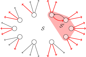
Figure 1: Diagrammatic representation of the sets $\mathcal{S}$ and $\mathcal{S}^{\prime}$ in algorithm 3 for $k=3$. Edges marked in red belong to set $\mathcal{D}^{+}$, i.e. the $2m$ directed pairs $(i,j)$ with smallest $\text{{d}}(i,j)$. Note that reciprocal edges need not both belong to $\mathcal{D}^{+}$, despite $\text{{d}}(i,j)$ being symmetric, since ties are broken arbitrarily. The nodes in red have all out-edges (nearest neighbors) in set $\mathcal{D}$, and hence are assigned to set $\mathcal{S}^{\prime}$. Since the set of $m$ best pairs could still contain undiscovered pairs of elements in $\mathcal{S}^{\prime}$, the search needs to continue recursively for members of this set.

In the above algorithm, the function $\text{{FindBest}}(m,\mathcal{S},\text{{d}})$ finds the set of $m$ pairs $(i,j)$ of elements in set $\mathcal{S}$ with the smallest “distance” $\textsc{d}(i,j)$ [which in our case corresponds to $-\max_{W_{ij}}\pi(\bm{W})$]. Clearly, for $\lfloor\kappa N\rceil>0$, if the original CD algorithm converges to the global optimum, so will the GCD algorithm. The function FindBest solves what is known as the $m$ closest pairs problem [32]. In that literature, $\textsc{d}(i,j)$ is often assumed to be a metric, typically euclidean, which allows the problem to be solved in log-linear time, usually by means of spacial sorting. However, this class of solution is not applicable to our case, since we cannot expect that our distance function will in general define a metric space. An exhaustive solution of this problem consists in probing all $|\mathcal{S}|\choose 2$ pairs, which would yield no improvement on the quadratic complexity of CD. Instead, we proceed by first solving the $m$ closest pairs problem with an algorithm proposed by Lenhof and Smid [33] that maps it to a recursive $k$-nearest neighbor (KNN) problem. The algorithm proceeds by setting $k={\lceil 4m/|\mathcal{S}|\rceil}$ and finding for each element $i$ in set $\mathcal{S}$ the $k$ nearest neighbors $j$ with smallest $\textsc{d}(i,j)$. From this set of directed pairs, we select the $2m$ best ones to compose the set $\mathcal{D}^{+}$, and construct a set $\mathcal{D}$ with the undirected version of the pairs in $\mathcal{D}^{+}$, such that $m\leq|\mathcal{D}|\leq 2m$. At this point we can identify a subset $\mathcal{S}^{\prime}$ of $\mathcal{S}$ composed of nodes for which all nearest neighbor edges belong to $\mathcal{D}$ when their direction is discarded, as shown in Fig. 1. Since these nodes have been saturated, we cannot rule out that the $m$ closest pairs will not contain undiscovered pairs of elements in set $\mathcal{S}^{\prime}$. Therefore, we proceed recursively for $\mathcal{S}^{\prime}$, and stop when $|\mathcal{S}|^{2}\leq 4m$, in which case the node set has become small enough for an exhaustive search to be performed. This is summarized as algorithm 3, and a proof of correctness is given in Ref. [33].

Algorithm 3 Find the $m$ best edge candidates.

FindBest$m,\mathcal{S},$d$|\mathcal{S}|^{2}\leq 4m$

$\{m$ pairs $(i,j)$ of nodes in set $\mathcal{S}$ with smallest $\textsc{d}(i,j)$ found by exhaustive search.$\}$ $\triangleright$ $O(|\mathcal{S}|^{2})$

$k\leftarrow{\lceil 4m/|\mathcal{S}|\rceil}$

$\bm{G}\leftarrow\text{FindKNN}(k,\mathcal{S},\text{{d}})$ $\triangleright$ $k$-nearest neighbor digraph

$\mathcal{D}^{+}\leftarrow 2m$ directed edges $(i,j)\in\bm{G}$ with smallest $\text{{d}}(i,j)$.

$\mathcal{D}\leftarrow$ unique undirected pairs $(i,j)$ in $\mathcal{D}^{+}$. $\triangleright$ $m\leq|\mathcal{D}|\leq 2m$

$\mathcal{S}^{\prime}\leftarrow\{i\in\mathcal{S}\,|\,(i,j)\in D,\forall\text{ out-neighbor $j$ of $i$ in $\bm{G}$.}\}$

$\mathcal{D}^{\prime}\leftarrow$ FindBest($m,\mathcal{S}^{\prime},$ d)

$\{\text{$m$ pairs $(i,j)$ in $\mathcal{D}\cup\mathcal{D}^{\prime}$ with smallest {d}$(i,j)$}\}$

As we will discuss in a moment, the recursion depth of algorithm 3 is bounded logarithmically on $|\mathcal{S}|$, and hence its runtime is dominated by the KNN search. Note that so far we have done nothing substantial to address the overall quadratic performance, since finding the $k$ nearest neighbors exhaustively still requires all pairs to be probed. Similarly to the $m$ closest pairs problem, efficient log-linear algorithms exist based on spacial sorting when the distance is euclidean, however more general approaches do also exist. In particular, the NNDescent algorithm by Dong et al [23] approximately solves the KNN problem in subquadratic time, while not requiring the distance function to be a metric. The algorithm is elegant, and requires no special data structure beyond the nearest neighbor graph itself, other than a heap for each node. It works by starting with a random KNN digraph, and successively updating the list of best neighbors by inspecting the neighbors of the neighbors in the undirected version of the KNN digraph, as summarized in algorithm 4. The main intuition behind this approach is that if $(i,j)$ and $(j,v)$ are good entries to update, then $(i,v)$ is likely to be a good candidate as well — even if triangle inequality is not actually obeyed.

Algorithm 4 Find $k$ nearest neighbors by NNDescent.

Input: Convergence criterion $\varepsilon$ FindKNN$k,\mathcal{V},$ d

$\bm{G}\leftarrow$ directed graph with node set $\mathcal{V}$ and $k$ out-neighbors chosen uniformly at random independently for all nodes.

$\Delta\leftarrow 0$

$\bm{G}^{\prime}\leftarrow\bm{G}$

$\bm{U}\leftarrow$ undirected version of $\bm{G}$ $i\in\mathcal{V}$ $j$ incident on $i$ in $\bm{U}$ $v$ incident on $j$ in $\bm{U}$ $v=i$ or $(i,v)\in\bm{G}^{\prime}$

continue

$\hat{u}\leftarrow\operatorname{arg\ max}_{u}\{\text{{d}}(i,u)\,|\,(i,u)\in\bm{G}^{\prime}\}$ $\triangleright$ (1) $\text{{d}}(i,v)<\text{{d}}(i,\hat{u})$

Replace $(i,\hat{u})$ with $(i,v)$ in $\bm{G}^{\prime}$ $\triangleright$ (2)

$\Delta\leftarrow\Delta+1$

$\bm{G}\leftarrow\bm{G}^{\prime}$ $\Delta/(k|\mathcal{V}|)<\varepsilon$

$\bm{G}$

(a) Random KNN graph	(b) Result of NNDescent	(c) Exact KNN graph

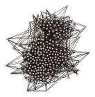
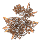
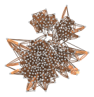
(d) Best $m$ updates via FindBest	(e) Exact best $m$ updates

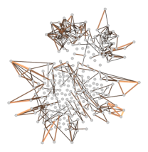
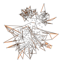
(f) Iterations of the GCD algorithm
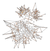
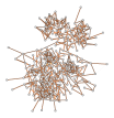
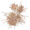
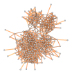
Iteration 1	Iteration 2	Iteration 3	Iteration 4

Figure 2: Example of our greedy coordinate descent algorithm for a covariance selection problem on a simulated dataset composed of $M=500$ samples given a network of friendships among high-school students [34]. The panels show intermediary results of the algorithm, starting from an empty network [i.e. $W_{ij}=0$ for all $(i,j)$]. The top row shows (a) the random initialization of NNDescent (algorithm 4) with $k=4$, (b) its final result, and (c) the exact result found with an exhaustive algorithm. The middle row shows (d) the result of the $m=\kappa N$ best updates using algorithm 3 with $\kappa=1$ and (e) the exact result according to an exhaustive algorithm. The edge colors indicate the value of $\max_{W_{ij}}\pi(\bm{W})$. The bottom row shows the first four iterations of the GCD algorithm.

Steps (1) and (2) in the algorithm can be both performed in time $O(1)$ by keeping a (e.g. Fibonacci) heap containing the nearest $k$ neighbors for each node. Thus, each full iteration of algorithm 4 runs in time $O(k^{2}N)$, assuming the degrees of nodes in $\bm{U}$ are all $O(k)$, otherwise it runs in time $O({\left<q\right>}N)$ where ${\left<q\right>}$ is the average number of second neighbors in $\bm{U}$. If ${\left<q\right>}\gg k^{2}$, the inner loops can be optionally constrained to run over only the first $k$ neighbors for each node, to preserve the $O(k^{2}N)$ complexity. Although this algorithm has seen wide deployment, in particular as part of the popular UMAP dimensionality reduction method [35], and has had its performance empirically “battle tested” in a variety of practical workloads, it has so far resisted a formal analysis of its algorithmic complexity. To date, the most careful analyses of this algorithm observe that the number of iterations required for convergence does not exceed $2\lceil\log_{2k}N\rceil$ in empirical settings [25]: The intuitive reasoning is that the initial random graph has as a diameter of approximately $\lceil\log_{2k}N\rceil$, and hence twice this is the number of steps needed for each node to communicate its neighborhood to all other nodes, and for the updated information to return. This estimated bound on the convergence results in an overall $O(k^{2}N\log N)$ complexity, which can be rigorously proven on a version of the algorithm where the second neighbor search is replaced by a range query, and the data is generated by a homogeneous Poisson process [24]. This typical log-linear complexity of the NNDescent algorithm is what finally enables us to escape the quadratic complexity of the CD algorithm, as we will demonstrate shortly.

Importantly, the NNDescent algorithm is approximative, as it does not guarantee that all nearest neighbors are always correctly identified. Although in practice it often yields very good recall rates [23], its inexact nature is not a concern for our purposes, since it does not affect the correctness of our GCD algorithm: if an element of the best set $\mathcal{E}_{\text{best}}$ in algorithm 2 is missed at a given iteration, it will eventually be considered in a future iteration, due to the random initialization of algorithm 4. Our primary concern is only with the average speed with which it finds the best update candidates. Nevertheless, as we show later, inaccuracies in the solution of the KNN problem often disappear completely by the time algorithm 3 finishes (as the KNN problem considers a much larger set of pairs than what gets eventually selected), such that the recall rates for the $m$ closest pairs problem approach the optimal values as the parameter $\kappa$ is increased.

In Fig 2 we show an example of the intermediate results obtained by our algorithm on simulated data on an empirical network.

In appendix B we list some low level optimizations that can improve the overall performance of the algorithm, including parallelization. A C++ implementation of the algorithm (with OpenMP CPU parallelism) is available as part of the graph-tool Python library [36].

III.1 Algorithmic complexity

We now obtain the overall algorithmic complexity of our GCD algorithm. At each iteration, algorithm 2 spends time $T(N,m)$ on algorithm 3 to find the $m=\kappa N$ best update coordinates, and time $O(\kappa N)$ to actually update them. Therefore, the overall algorithmic complexity will be given by $T(N,\kappa N)$, since this is bounded from below by $\kappa N$.

When using NNDescent, algorithm 3 has a complexity given recursively by

$$T(N,m)=O(k^{2}N\log N+m\log m)+T(|\mathcal{S}^{\prime}|,m),$$ (6)

with $k={\lceil 4m/N\rceil}$, and boundary condition $T(N,m)=O(N^{2})$ if $N^{2}\leq 4m$. In general, ignoring an overall multiplicative constant, we can write

$$T(N,m)=\sum_{t=0}^{r}\frac{m^{2}}{N_{t}}\log N_{t}+(r+1)m\log m+O(m)\\$$ (7)

where $N_{t}=|\mathcal{S}_{t-1}^{\prime}|$ is the number of nodes being considered at recursion $t$, with $\mathcal{S}_{t}^{\prime}$ being the set $\mathcal{S}^{\prime}$ at recursion $t$ (assuming $\mathcal{S}_{-1}^{\prime}=\mathcal{V}$), and $t=r+1$ is the first point at which $N_{t}\leq 2\sqrt{m}$, and hence the final recursion runs in time $O(m)$. Introducing $s_{t}=N_{t}/N$ as the fraction of nodes at recursion $t$, we can write

$$T(N,\kappa N)=\kappa^{2}N\left[(\log N)\sum_{t=0}^{r}\frac{1}{s_{t}}+\sum_{t=0}^{r}\frac{\log s_{t}}{s_{t}}\right]\\ +(r+1)\kappa N\log\kappa N+O(\kappa N).$$ (8)

Since $\log s_{t}\leq 0$ and $1/s_{t}\geq 1$, this will lead to an overall complexity of

$$T(N,\kappa N)=O\left[\left(\sum_{t=0}^{r}\frac{1}{s_{t}}\right)\kappa^{2}N\log N\right].$$ (9)

The prefactor in the above expression will in general depend on the data and the stage of the algorithm, as we will see.

We can obtain a loose upper bound to the running time by assuming the worst-case where the progression of the algorithm is (in principle) the slowest. We first observe that we must always have $s_{t}\leq 1/2^{t}$, i.e. the number of nodes being considered must decay at least exponentially fast with each recursion. This is because in algorithm 3 we have that $|\mathcal{D}^{+}_{t}|\geq k|\mathcal{S}^{\prime}_{t}|$ and $|\mathcal{D}^{+}_{t}|=2m$, and thus $N_{t+1}=|\mathcal{S}^{\prime}_{t}|\leq 2m/k=2m/{\lceil 4m/N_{t}\rceil}\leq N_{t}/2$, and hence $s_{t+1}\leq s_{t}/2$, which leads to $s_{t}\leq 1/2^{t}$ since $s_{0}=1$. Therefore, the worst case is $s_{t}=1/2^{t}$, giving us $\sum_{t=0}^{r}1/s_{t}=\sum_{t=0}^{r}2^{t}=2^{r+1}-1$, and $2^{r+1}=\sqrt{N/4\kappa}$, and hence a complexity of

$$T(N,\kappa N)=O(\kappa^{3/2}N^{3/2}\log N).$$ (10)

However, although already subquadratic, this upper bound is not tight. This is because it is not in fact possible for the worst case $s_{t}=1/2^{t}$ to be realized at every recursion, and in fact the number of nodes being considered will generically decrease faster than exponentially. We notice this by performing a more detailed analysis of the runtime, as follows.

Let $\bm{A}$ be the graph consisting of $N$ nodes and the $m$ closest pairs we want to find as edges. Further, let $P(d)$ be the degree distribution of $\bm{A}$ (i.e. the fraction of nodes with degree $d$), and $F(d)=\sum_{d^{\prime}=d}^{\infty}P(d^{\prime})$ the tail cumulative distribution function of $P(d)$. At recursion $t$ we discover at most $k_{t}={\lceil 4m/N_{t}\rceil}={\lceil 4\kappa/s_{t}\rceil}$ neighbors of each node in $\bm{A}$. Therefore, every node in $\bm{A}$ with degree $d\geq k_{t}$ will belong to set $\mathcal{S}^{\prime}_{t}$ and be considered for next recursion $t+1$. This means we can write

$$N_{t+1}=NF(k_{t}),$$ (11)

and dividing by $N$ on both sides leads to

$$s_{t+1}=F({\lceil 4\kappa/s_{t}\rceil}),$$ (12)

which no longer depends on $N$.

At this point we can see why the worst case $s_{t}=1/2^{t}$ considered for the upper bound above is strictly impossible: it would correspond to $F(d)=2\kappa/d$ for $d\geq 4\kappa$ (this can be verified by inserting $F(d)$ in Eq. 12 and iterating) which is incompatible with the mean of $P(d)$ being finite and equal to $2\kappa$ — a requirement of the graph $\bm{A}$ having $N$ nodes and $m=\kappa N$ edges. We notice this by writing the mean as $2\kappa=\sum_{d}dP(d)=\sum_{d}d[F(d)-F(d+1)]=\sum_{d}F(d)-1$, and the fact that the sum $\sum_{d=4\kappa}^{\infty}1/d$ diverges.

Given some valid $F(d)$ we can obtain the prefactor in Eq. 9 using the fact that the algorithm terminates when $s_{r+1}\leq\sqrt{4\kappa/N}$, and therefore we can recursively invert Eq. 12 as

$$\frac{1}{s_{r}} =\frac{F^{-1}(\sqrt{4\kappa/N})}{4\kappa}$$ (13)

$$\frac{1}{s_{t}} =\frac{F^{-1}(s_{t+1})}{4\kappa},\qquad(\text{for }0<t<r).$$ (14)

The recursion depth and fraction of nodes considered will depend on the degree distribution of $\bm{A}$ via $F^{-1}(z)$, and therefore it will vary for different instances of the problem. We consider a few cases as examples of the range of possibilities.

The first case is when $\bm{A}$ is a $d$-regular graph, i.e. every node has degree exactly $2\kappa$ (assuming it is an integer), corresponding to the extreme case of maximum homogeneity. This gives us $F(d)=\{1\text{ if }d\leq 2\kappa,\;0\text{ otherwise}\}$, and therefore it follows directly from Eq. 12 that $s_{t}=0$ for $t>0$, and hence the overall complexity becomes simply

$$T(N,\kappa N)=O(\kappa^{2}N\log N),$$ (15)

corresponding to a single call of the KNN algorithm.

Moving to a case with intermediary heterogeneity, let us consider a geometric distribution $P(d)=(1-p)^{d}p$, with $(1-p)/p=2\kappa$, which gives us $F(d)=[2\kappa/(2\kappa+1)]^{d}$, and $F^{-1}(z)=\log z/\log[2\kappa/(2\kappa+1)]$. Inserting this in Eq. 14 gives us

$$\frac{1}{s_{r}} =\frac{\log\sqrt{N/(4\kappa)}}{4\kappa\log[(2\kappa+1)/(2\kappa)]}=O(\log N)$$ (16)

$$\frac{1}{s_{r-1}} =\frac{\log 1/s_{r}}{4\kappa\log[(2\kappa+1)/(2\kappa)]}=O(\log\log N)$$ (17)

$$\frac{1}{s_{r-2}} =\frac{\log 1/s_{r-1}}{4\kappa\log[(2\kappa+1)/(2\kappa)]}=O(\log\log\log N),$$ (18)

and so on, such that the term $1/s_{r}$ dominates, giving us an overall log-linear complexity

$$T(N,\kappa N)=O(\kappa^{2}N\log^{2}N).$$ (19)

This result means that for relatively more heterogeneous degree distributions we accrue only an additional $\log N$ factor in comparison to the $d$-regular case, and remain fairly below the upper bound found previously.

Based on the above, we can expect broader degree distributions in $\bm{A}$ to cause longer run times. A more extreme case is given by the Zipf distribution $P(d)=d^{-\alpha}/\zeta(\alpha)$, where $\zeta(\alpha)$ is the Riemann zeta function, with $\alpha$ chosen so that the mean is $2\kappa$. In this case we can approximate $F(d)=\sum_{d^{\prime}=d}^{\infty}P(d)\approx\zeta(\alpha)^{-1}\int_{d}^{\infty}x^{-\alpha}\mathrm{d}x\propto d^{1-\alpha}$, and $F^{-1}(z)\propto z^{1/(1-\alpha)}$. Substituting above in Eq. 14 we get

$$\frac{1}{s_{r}} =\frac{\left(\sqrt{4\kappa/N}\right)^{\frac{1}{1-\alpha}}}{4\kappa}=O\left(\kappa^{\frac{1}{2(1-\alpha)}-1}N^{\frac{1}{2(\alpha-1)}}\right)$$ (20)

$$\frac{1}{s_{r-1}} =\frac{\left(1/s_{r}\right)^{\frac{1}{\alpha-1}}}{4\kappa}=O\left(\kappa^{\frac{1}{2(1-\alpha)}-2}N^{\frac{1}{2(\alpha-1)^{2}}}\right)$$ (21)

$$\frac{1}{s_{r-\ell}} =\frac{\left(1/s_{r-\ell+1}\right)^{\frac{1}{\alpha-1}}}{4\kappa}=O\left(\kappa^{\frac{1}{2(1-\alpha)}-\ell-1}N^{\frac{1}{2(\alpha-1)^{\ell+1}}}\right),$$ (22)

which is again dominated by $1/s_{r}$, and hence gives us

$$T(N,\kappa N)=O(\kappa^{1-\frac{1}{2(\alpha-1)}}N^{1+\frac{1}{2(\alpha-1)}}\log N).$$ (23)

The value of $\alpha$ is not a free parameter, since it needs to be compatible with the mean degree $2\kappa$. For very large $2\kappa\gg 1$ we have that $\alpha\to 2$, and hence the complexity will be asymptotically similar to the upper bound we found previously, i.e.

$$T(N,\kappa N)=O(\kappa^{1/2}N^{3/2}\log N),$$ (24)

although this is not how the algorithm is realistically evoked, as we need $\kappa=O(1)$ for a reasonable performance. For example, if $\alpha=5/2$ we have $2\kappa\approx 1.947$, and hence a complexity of $O(\kappa^{2/3}N^{4/3}\log N)$, and for low $2\kappa\to 1$ we have $\alpha\to\infty$, yielding the lower limit

$$T(N,N/2)=O(N\log N),$$ (25)

compatible with the $d$-regular case for $d=1$, as expected. Therefore, even in such an extremely heterogeneous case, the complexity remains close to log-linear for reasonably small values of $\kappa$.

We emphasize that the graph $\bm{A}$ considered for the complexity analysis above is distinct from the final network $\bm{W}$ we want to reconstruct. The latter might have an arbitrary structure, but the graph $\bm{A}$ represents only the updates that need to be performed, and it has a density which controlled by the parameter $\kappa$ of our algorithm. Thus, even if $\bm{W}$ has a very broad degree distribution, the one we see in $\bm{A}$ will be further limited by the parameter $\kappa$ and which updates are needed by the GCD algorithm [for an example, compare panels (d) and (f) in Fig. 2].

IV Performance assessment

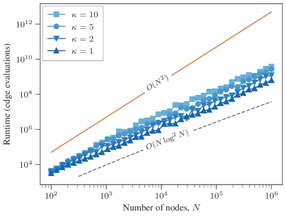
Figure 3: Runtime of the FindBest function (algorithm 3), for different values of $\kappa$, on $M=10$ samples of a multivariate Gaussian (see Appendix A) on $N$ nodes and nonzero entries of $\bm{W}$ sampled as an Erdős-Rényi graph with mean degree $5$ and nonzero weights independently normally sampled with mean $-10^{3}$ and standard deviation 10, and diagonal entries $W_{ii}=\sum_{j\neq i}|W_{ij}|/(1-\epsilon)^{2}$ with $\epsilon=10^{-3}$. The results show averages over $10$ independent problem instances.

(a) Brazilian congress votes [37]	(b) Ocean microbiome [38]
($N=882$, Ising model)	($N=35,651$, Ising model)
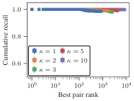
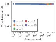
(c) Rat gene co-expression [39]	(d) Microbiome (elbow joint) [40]
($N=13,751$, Multiv. Gaussian)	($N=10,242$, Ising model)

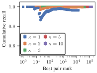
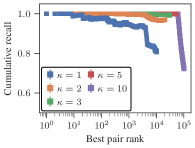
Figure 4: Cumulative recall rates for the FindBest function for different values of $\kappa$ on a variety of empirical data and reconstruction objectives, as shown in the legend (see Appendix A). The results shows averages over 10 runs of the algorithm.

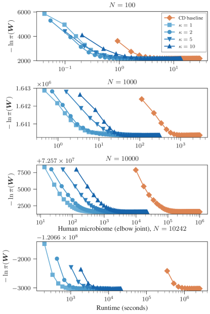
Figure 5: Convergence of the CD and GCD algorithms for artificial data sampled from a multivariate Gaussian (same parameterization as Fig. 3 but with $M=100$ samples) for three different values of the number of nodes $N$ and values of $\kappa$, together with the CD baseline. The bottom panel shows the results obtained for empirical data for the human microbiome samples of the elbow joint, using the Ising model.

(a) Earth microbiome	(b) Human microbiome	(c) Nematode gene expression
($N=317,314$, $M=23,828$)	($N=45,383$, $M=4,788$)	($N=17,256$, $M=1,357$)

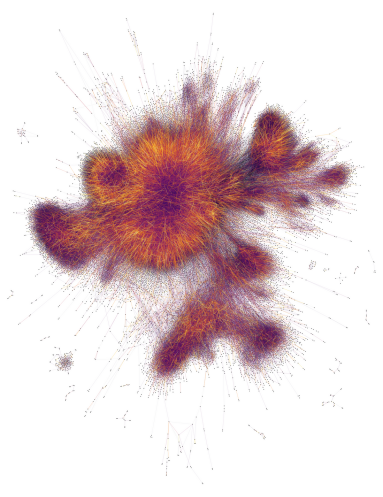
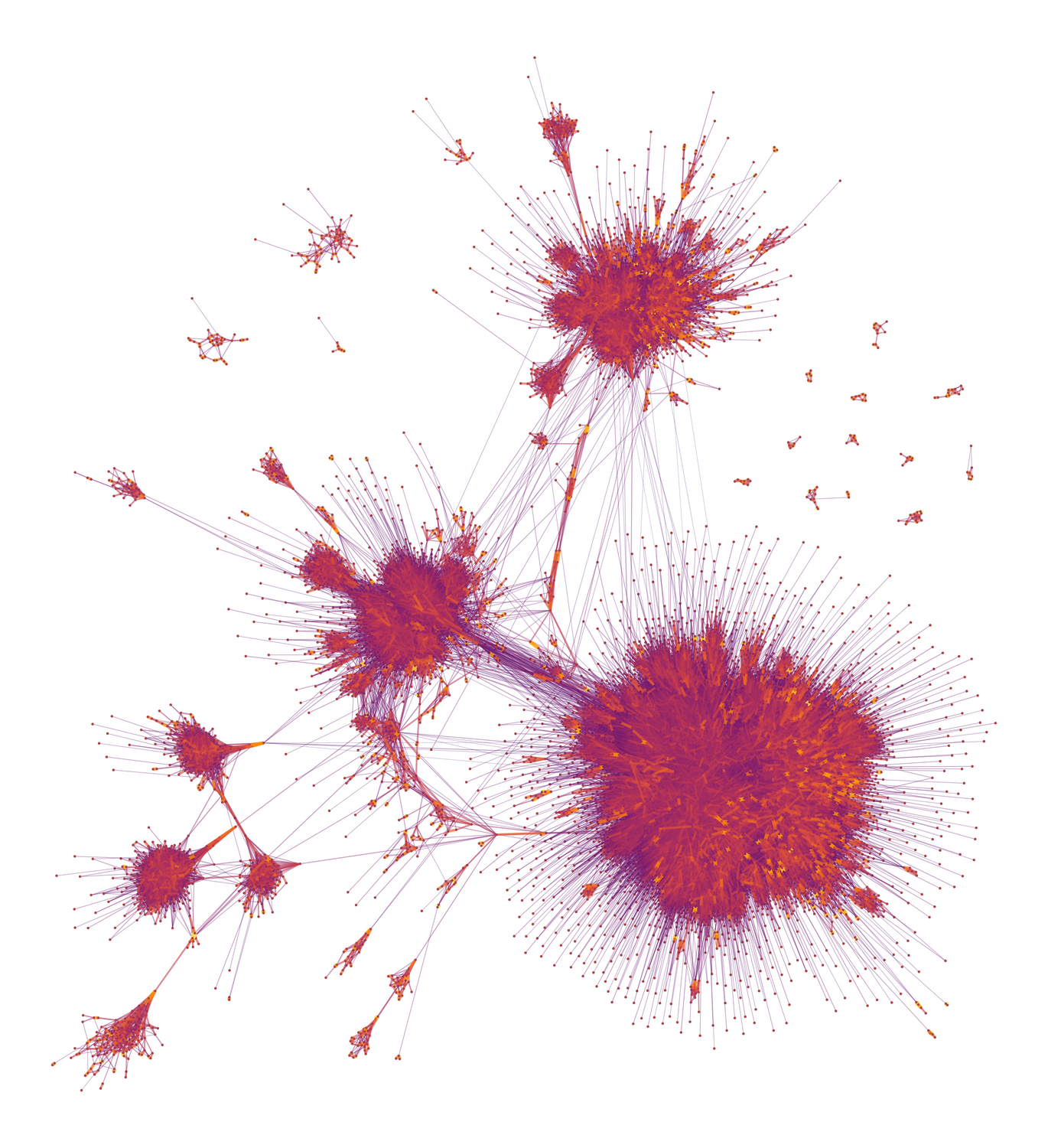
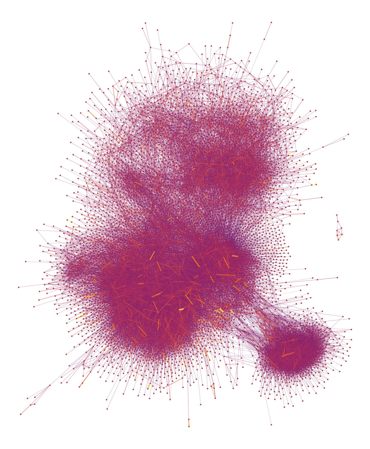
Figure 6: Reconstructed networks for the empirical datasets described in the text, as shown in the legend, using the Ising model for (a) and (b), and multivariate Gaussian for (c). The edge colors indicate the magnitude of the entries of the $\bm{W}$ matrix. Nodes with degree zero were excluded from the visualization.

We now conduct an analysis of the performance of our algorithm in a variety of artificial and empirical settings. We begin with an analysis of the runtime of the FindBest function (algorithm 3) on $M=10$ samples of a multivariate Gaussian (see Appendix A) on $N$ nodes and nonzero entries of $\bm{W}$ sampled as an Erdős-Rényi graph with mean degree $5$. As we see in Fig. 3, the runtime of the algorithm is consistent with a $O(N\log^{2}N)$ scaling as obtained theoretically in the previous section for a homogeneous update graph.

This kind of log-linear performance is promising for the scalability of the overall algorithm, but it stills needs to be determined if the results of FindBest are sufficiently accurate for a speedy progression of the GCD algorithm. In Fig. 4 we show the cumulative recall rates of the exact best pairs obtained with an exhaustive algorithm, defined as the fraction of best pairs correctly identified up to a given rank position (with the best pair having rank 1), for a variety of empirical data. We observe in general very good recall rates, compatible with what is obtained with the NNDescent algorithm [23]. Importantly, in every case we considered, we observed that the cumulative recall values start at $1$, meaning that the first best edges are always correctly identified. For some data, the algorithm may falter slightly for intermediary pairs and a low $\kappa$, but increasing $\kappa$ has the systematic effect of substantially improving the recall rates (at the expense of longer runtimes). We emphasize again that it is not strictly necessary for the FindBest function to return exact results, since it will be called multiple times during the GCD loop, and its random initialization guarantees that every pair will eventually be considered — it needs only to be able to locate the best edge candidates with high probability. Combined with the previous result of Fig. 3, this indicates that the fast runtime of the FindBest function succeeds in providing the GCD algorithm with the entries of the $\bm{W}$ matrix that are most likely to improve the objective function, while avoiding an exhaustive $O(N^{2})$ search.

We can finally evaluate the final performance of the GCD algorithm by its convergence speed, as shown in Fig. 5 for artificial and empirical data. For a small data with $N=100$ we observe only a modest improvement over the CD baseline, but this quickly improves for larger $N$: For $N=1,000$ we already observe a $100\times$ runtime improvement, which increases to $1,000\times$ for $N=10,000$. Interestingly, we observe that the $\kappa=1$ results show the fastest convergence, indicating that the decreased accuracy of the FindBest function — resulting in it needing to be called more often — is compensated by its improved runtime. For $\kappa=10$ we see that the speed of convergence per iteration is virtually the same as the CD baseline, but it significantly outperforms it in real time. This seems to demonstrate that, as expected for the reconstruction of a sparse network, most $O(N^{2})$ updates performed by the CD baseline algorithm are wasteful, and only a $O(N)$ subset is actually needed at each stage for the actual progression of the algorithm — which the FindBest function is capable of identifying in subquadratic time.

The results above are representative of what we have observed on a larger set of empirical data (not shown). We were not able to find a single instance of an empirical or artificial scenario that contradicts the log-linear runtime of the FindBest function, or where our algorithm does not provide a significant improvement over the $O(N^{2})$ CD baseline (except for very small $N$).

V Empirical examples

We demonstrate the use of our algorithm with a few large scale datasets, which would be costly to analyze with a quadratic reconstruction algorithm. We showcase on the following:

Earth microbiome project [41].

A collection of crowd-sourced microbial samples from various biomes and habitats across the globe, containing abundances of operational taxonomic units (OTU), obtained via DNA sequencing and mass spectrometry. An OTU is a proxy for a microbial species, and a single sample consists of the abundances of each OTU measured at the same time. This dataset consists of $M=23,828$ samples involving $N=317,314$ OTUs.

Human microbiome project [40].

A collection of microbial samples from 300 healthy adults between the ages of 18 and 40, collected at five major body sites (oral cavity, nasal cavity, skin, gastrointestinal tract and urogenital tract) with a total of 15 or 18 specific body sites. The abundances of OTUs were obtained using 16S rRNA and whole metagenome shotgun (mWGS) sequencing. This dataset consists of $M=4,788$ samples involving $N=45,383$ OTUs.

For both co-occurrence datasets above, we binarized each sample as $x_{i}\in\{-1,1\}$, for absence and presence, respectively, and used the Ising model for the network reconstruction (see Appendix A). In this case, the matrix $\bm{W}$ yields the strength of the coupling between two OTUs, and a value $W_{ij}=0$ means that OTUs $i$ and $j$ are conditionally independent from one another.

Animal gene expression database COXPRESdb [39].

This database consists of genome-wide gene expression reads for 10 animal species as well as budding and fission yeast. Each gene expression sample was obtained using RNAseq, with read counts converted to base-2 logarithms after adding a pseudo-count of $0.125$, and batch corrected using Combat [42]. We used the nematode dataset, consisting of $M=1,357$ samples of $N=17,256$ genes. For this dataset we used the multivariate Gaussian model (see Appendix. A), where the matrix $\bm{W}$ corresponds to the inverse covariance between gene expression levels (a.k.a. precision matrix). In this case, the partial correlation between two genes, i.e. their degree of association controlling for all other genes, is given by $-W_{ij}/\sqrt{W_{ii}W_{jj}}$, so that gene pairs with $W_{ij}=0$ are conditionally independent.

The reconstructed networks for all three datasets are shown in Fig. 6. They all seem to display prominent modular structure. In the case of microbial co-occurrence datasets the clusters correspond mostly to different habitats and geographical regions for the earth microbiome, and to different body sites for the human microbiome.

VI Conclusion

We have described a method to reconstruct interaction networks from observational data that avoids a seemingly inherent quadratic complexity on the number of nodes, in favor of a data-dependent runtime that is typically log-linear. Our algorithm does not rely on particular formulations of the reconstruction problem, other than the updates on the edge weights being done in constant time with respect to the total number of nodes. Together with its straightforward parallelizability, our proposed method removes a central barrier to the reconstruction of large-scale networks, and can be applied to problems with a number of nodes and edges on the order of hundreds of thousands, millions, or potentially even more depending on available computing resources.

Our algorithm relies on the NNDescent [23] approach for approximate $k$-nearest neighbor search. Despite the robust empirical evidence for its performance, a detailed theoretical analysis of this algorithm is still lacking, in particular of its potential modes of failures. We expect further progress in this direction to elucidate potential limitations and improvements to our overall approach.

In this work we focused on convex reconstruction objectives, such as the inverse Ising model and multivariate Gaussian with $L_{1}$ regularization. More robust regularization schemes or different models may no longer be convex, in which case coordinate descent will fail in general at converging to the global optimum. However, it is clear that our strategy of finding the best edge candidates in subquadratic time is also applicable for algorithms that can be used with nonconvex objectives, such as stochastic gradient descent or simulated annealing. We leave such extensions for future work.

VII Acknowledgments

Sample processing, sequencing, and core amplicon data analysis were performed by the Earth Microbiome Project (http://www.earthmicrobiome.org), and all amplicon sequence data and metadata have been made public through the EMP data portal (http://qiita.microbio.me/emp).

Appendix A Generative models

In our examples we use two graphical models: the Ising model [17] and a multivariate Gaussian distribution [12]. The Ising model is a distribution on $N$ binary variables $\bm{x}\in\{-1,1\}^{N}$ given by

$$P(\bm{x}|\bm{W},\bm{\theta})=\frac{\mathrm{e}^{\sum_{i<j}W_{ij}x_{i}x_{j}+\sum_{i}\theta_{i}x_{i}}}{Z(\bm{W},\bm{\theta})},$$ (26)

with $\theta_{i}$ being a local field on node $i$, and $Z(\bm{W},\bm{\theta})=\sum_{\bm{x}}\mathrm{e}^{\sum_{i<j}W_{ij}x_{i}x_{j}+\sum_{i}\theta_{i}x_{i}}$ a normalization constant. Since this normalization cannot be computed in closed form, we make use of the pseudolikelihood approximation [43],

$$P(\bm{x}|\bm{W},\bm{\theta}) =\prod_{i}P(x_{i}|\bm{x}\setminus{x_{i}},\bm{W},\bm{\theta})$$ (27)

$$=\prod_{i}\frac{\mathrm{e}^{x_{i}(\sum_{j}W_{ij}x_{j}+\theta_{i})}}{2\cosh(\sum_{j}W_{ij}x_{j}+\theta_{i})},$$ (28)

as it gives asymptotically correct results and has excellent performance in practice [17]. Likewise, the (zero-mean) multivariate Gaussian is a distribution on $\bm{x}\in\mathbb{R}^{N}$ given by

$$P(\bm{x}|\bm{W})=\frac{\mathrm{e}^{-\frac{1}{2}{\bm{x}}^{\top}\bm{W}\bm{x}}}{\sqrt{(2\pi)^{N}|\bm{W}^{-1}|}},$$ (29)

where $\bm{W}$ is the precision (or inverse covariance) matrix. Unlike the Ising model, this likelihood is analytical — nevertheless, the evaluation of the determinant is computationally expensive, and therefore we make use of the same pseudolikelihood approximation [44],

$$P(\bm{x}|\bm{W},\bm{\theta})=\prod_{i}\frac{\mathrm{e}^{-(x_{i}+\theta_{i}^{2}\sum_{j\neq i}W_{ij}x_{j})^{2}/2\theta_{i}^{2}}}{\sqrt{(2\pi)}\theta_{i}},$$ (30)

where we parameterize the diagonal entries as $\theta_{i}=1/\sqrt{W_{ii}}$.

In both cases, we have an additional set of $N$ parameters $\bm{\theta}$ which we update alongside the matrix $\bm{W}$ in our algorithms. Updates on an individual entry $W_{ij}$ of $\bm{W}$ can be computed in time $O(1)$ (independently of the degrees of $i$ and $j$ in a sparse representation of $\bm{W}$) by keeping track of the weighted sum of the neighbors $m_{i}=\sum_{j\neq i}W_{ij}x_{j}$ for every node and updating it as appropriate.

For both models we use a Laplace prior

$$P(\bm{W}|\lambda)=\prod_{i<j}\lambda\mathrm{e}^{-\lambda|W_{ij}|}/2,$$ (31)

which provides a convex $L_{1}$ regularization with a penalty given by $\lambda$, chosen to achieve a desired level of sparsity.

Appendix B Low-level optimizations

Below we describe a few low-level optimizations that we found to give good improvements to the runtime of the algorithm we propose in the main text.

Caching.

The typical case for objective functions $\pi(\bm{W})$ is that the computation of $\max_{W_{ij}}\pi(\bm{W})$ will require $O(M)$ operations, where $M$ is the number of data samples available. Since this computation is done in the innermost loops of algorithm 4, it will amount to an overall multiplicative factor of $O(M)$ in its runtime. However, because the distance function $\textsc{d}(i,j)$ will be called multiple times for the same pair $(i,j)$, a good optimization strategy is to cache its values, for example in a hash table, such that repeated calls will take time $O(1)$ rather than $O(M)$. We find that this optimization can reduce the total runtime of algorithm 4 by at least one order of magnitude in typical cases.

Gradient as distance.

The definition of $\textsc{d}(i,j)=-\max_{W_{ij}}\pi(\bm{W})$ is sufficient to guarantee the correctness of the algorithm 3, but in situations where it cannot be computed in closed form, requiring for example a bisection search, a faster approach is to use instead the absolute gradient $\textsc{d}(i,j)=-|\frac{\partial}{\partial W_{ij}}\log\pi(\bm{W})|$, which often can be analytically computed or well approximated with finite difference. In general this requires substantially fewer likelihood evaluations than bisection search. This approach is strictly applicable only with differentiable objectives, although we observed correct behavior for $L_{1}$-regularized likelihoods when approximating the gradient using central finite difference. We observed that this optimization improves the runtime by a factor of around six in typical scenarios.

Parallelization.

The workhorse of the algorithm is the NNDescent search (algorithm  4), which is easily parallelizable in a shared memory environment, since the neighborhood of each node can be inspected, and its list of nearest neighbors can be updated, in a manner that is completely independent from the other nodes, and hence requires no synchronization. Thus, the parallel execution of algorithm 4 is straightforward.

The actual updates of the matrix $\bm{W}$ in the GCD algorithm 2 can also be done in parallel, but that requires some synchronization. For many objectives $\pi(\bm{W})$, we can only consider the change of one value $W_{ij}$ at a time for each node $i$ and $j$, since the likelihood will involve sums of the type $m_{i}=\sum_{j}W_{ij}x_{j}$ for a node $i$, where $x_{j}$ are data values. Therefore, only the subset of the edges $\mathcal{E}_{\text{best}}$ in algorithm 2 that are incident to an independent vertex set in the graph will be able to be updated in parallel. This can be implemented with mutexes on each node, which are simultaneously locked by each thread (without blocking) for each pair $(i,j)$ before $W_{ij}$ is updated, which otherwise proceeds to the next pair if the lock cannot be acquired. Empirically, we found that is enough to keep up to 256 threads busy with little contention for $N>10^{4}$ with our OpenMP implementation [36].

References

- Lauritzen [1996] S. L. Lauritzen, Graphical Models, Vol. 17 (Clarendon Press, 1996).
- Jordan [2004] M. I. Jordan, Graphical Models, Statistical Science 19, 140 (2004).
- Drton and Maathuis [2017] M. Drton and M. H. Maathuis, Structure Learning in Graphical Modeling, Annual Review of Statistics and Its Application 4, 365 (2017).
- Timme and Casadiego [2014] M. Timme and J. Casadiego, Revealing networks from dynamics: An introduction, Journal of Physics A: Mathematical and Theoretical 47, 343001 (2014).
- Hallac et al. [2017] D. Hallac, Y. Park, S. Boyd, and J. Leskovec, Network Inference via the Time-Varying Graphical Lasso (2017), arxiv:1703.01958 [cs, math] .
- Guseva et al. [2022] K. Guseva, S. Darcy, E. Simon, L. V. Alteio, A. Montesinos-Navarro, and C. Kaiser, From diversity to complexity: Microbial networks in soils, Soil Biology and Biochemistry 169, 108604 (2022).
- Bury [2013] T. Bury, A statistical physics perspective on criticality in financial markets, Journal of Statistical Mechanics: Theory and Experiment 2013, P11004 (2013), arxiv:1310.2446 [physics, q-fin] .
- Weigt et al. [2009] M. Weigt, R. A. White, H. Szurmant, J. A. Hoch, and T. Hwa, Identification of direct residue contacts in protein–protein interaction by message passing, Proceedings of the National Academy of Sciences 106, 67 (2009).
- D’haeseleer et al. [2000] P. D’haeseleer, S. Liang, and R. Somogyi, Genetic network inference: From co-expression clustering to reverse engineering, Bioinformatics 16, 707 (2000).
- Manning et al. [2014] J. R. Manning, R. Ranganath, K. A. Norman, and D. M. Blei, Topographic Factor Analysis: A Bayesian Model for Inferring Brain Networks from Neural Data, PLOS ONE 9, e94914 (2014).
- Braunstein Alfredo et al. [2019] Braunstein Alfredo, Ingrosso Alessandro, and Muntoni Anna Paola, Network reconstruction from infection cascades, Journal of The Royal Society Interface 16, 20180844 (2019).
- Dempster [1972] A. P. Dempster, Covariance Selection, Biometrics 28, 157 (1972), 2528966 .
- Friedman et al. [2008] J. Friedman, T. Hastie, and R. Tibshirani, Sparse inverse covariance estimation with the graphical lasso, Biostatistics 9, 432 (2008).
- Mazumder and Hastie [2012] R. Mazumder and T. Hastie, The graphical lasso: New insights and alternatives, Electronic Journal of Statistics 6, 2125 (2012).
- Hastie et al. [2015] T. Hastie, R. Tibshirani, and M. Wainwright, Statistical Learning with Sparsity: The Lasso and Generalizations (CRC Press, 2015).
- Bresler et al. [2008] G. Bresler, E. Mossel, and A. Sly, Reconstruction of Markov Random Fields from Samples: Some Observations and Algorithms, in Approximation, Randomization and Combinatorial Optimization. Algorithms and Techniques, Lecture Notes in Computer Science (Springer, Berlin, Heidelberg, 2008) pp. 343–356.
- Nguyen et al. [2017] H. C. Nguyen, R. Zecchina, and J. Berg, Inverse statistical problems: From the inverse Ising problem to data science, Advances in Physics 66, 197 (2017).
- Hsieh et al. [2014] C.-J. Hsieh, M. A. Sustik, I. S. Dhillon, and P. Ravikumar, QUIC: Quadratic Approximation for Sparse Inverse Covariance Estimation, Journal of Machine Learning Research 15, 2911 (2014).
- Hsieh et al. [2013] C.-J. Hsieh, M. A. Sustik, I. S. Dhillon, P. K. Ravikumar, and R. Poldrack, BIG & QUIC: Sparse Inverse Covariance Estimation for a Million Variables, in Advances in Neural Information Processing Systems, Vol. 26 (Curran Associates, Inc., 2013).
- Bresler [2015] G. Bresler, Efficiently Learning Ising Models on Arbitrary Graphs, in Proceedings of the Forty-seventh Annual ACM Symposium on Theory of Computing, STOC ’15 (ACM, New York, NY, USA, 2015) pp. 771–782.
- Bresler et al. [2010] G. Bresler, E. Mossel, and A. Sly, Reconstruction of Markov Random Fields from Samples: Some Easy Observations and Algorithms (2010), arxiv:0712.1402 [cs] .
- Bresler et al. [2018] G. Bresler, D. Gamarnik, and D. Shah, Learning Graphical Models From the Glauber Dynamics, IEEE Transactions on Information Theory 64, 4072 (2018).
- Dong et al. [2011] W. Dong, C. Moses, and K. Li, Efficient k-nearest neighbor graph construction for generic similarity measures, in Proceedings of the 20th International Conference on World Wide Web, WWW ’11 (Association for Computing Machinery, New York, NY, USA, 2011) pp. 577–586.
- Baron and Darling [2020] J. D. Baron and R. W. R. Darling, K-Nearest Neighbor Approximation Via the Friend-of-a-Friend Principle (2020), arxiv:1908.07645 [math, stat] .
- Baron and Darling [2022] J. D. Baron and R. W. R. Darling, Empirical complexity of comparator-based nearest neighbor descent (2022), arxiv:2202.00517 [cs, stat] .
- Wright [2015] S. J. Wright, Coordinate descent algorithms, Mathematical Programming 151, 3 (2015).
- Spall [2012] J. C. Spall, Cyclic Seesaw Process for Optimization and Identification, Journal of Optimization Theory and Applications 154, 187 (2012).
- Abbeel et al. [2006] P. Abbeel, D. Koller, and A. Y. Ng, Learning Factor Graphs in Polynomial Time and Sample Complexity, Journal of Machine Learning Research 7, 1743 (2006).
- Wainwright et al. [2006] M. J. Wainwright, J. Lafferty, and P. Ravikumar, High-Dimensional Graphical Model Selection Using $\ell_1$-Regularized Logistic Regression, in Advances in Neural Information Processing Systems, Vol. 19 (MIT Press, 2006).
- Santhanam and Wainwright [2009] N. Santhanam and M. J. Wainwright, Information-theoretic limits of selecting binary graphical models in high dimensions (2009), arxiv:0905.2639 [cs, math, stat] .
- Santhanam and Wainwright [2008] N. Santhanam and M. J. Wainwright, Sample complexity of determining structures of graphical models, in 2008 46th Annual Allerton Conference on Communication, Control, and Computing (2008) pp. 1232–1237.
- Smid [2000] M. Smid, Closest-Point Problems in Computational Geometry, in Handbook of Computational Geometry, edited by J. R. Sack and J. Urrutia (North-Holland, Amsterdam, 2000) pp. 877–935.
- Lenhof and Smid [1992] H.-P. Lenhof and M. Smid, The k closest pairs problem, Unpublished manuscript (1992).
- Moody [2001] J. Moody, Race, School Integration, and Friendship Segregation in America, American Journal of Sociology 107, 679 (2001).
- McInnes et al. [2018] L. McInnes, J. Healy, and J. Melville, UMAP: Uniform Manifold Approximation and Projection for Dimension Reduction, arXiv:1802.03426 [cs, stat] (2018), arxiv:1802.03426 [cs, stat] .
- Peixoto [2014] T. P. Peixoto, The graph-tool python library, figshare 10.6084/m9.figshare.1164194 (2014), available at https://graph-tool.skewed.de.
- Peixoto [2019] T. P. Peixoto, Network Reconstruction and Community Detection from Dynamics, Physical Review Letters 123, 128301 (2019).
- Sunagawa et al. [2015] S. Sunagawa, L. P. Coelho, S. Chaffron, J. R. Kultima, K. Labadie, G. Salazar, B. Djahanschiri, G. Zeller, D. R. Mende, A. Alberti, F. M. Cornejo-Castillo, P. I. Costea, C. Cruaud, F. d’Ovidio, S. Engelen, I. Ferrera, J. M. Gasol, L. Guidi, F. Hildebrand, F. Kokoszka, C. Lepoivre, G. Lima-Mendez, J. Poulain, B. T. Poulos, M. Royo-Llonch, H. Sarmento, S. Vieira-Silva, C. Dimier, M. Picheral, S. Searson, S. Kandels-Lewis, Tara Oceans coordinators, C. Bowler, C. de Vargas, G. Gorsky, N. Grimsley, P. Hingamp, D. Iudicone, O. Jaillon, F. Not, H. Ogata, S. Pesant, S. Speich, L. Stemmann, M. B. Sullivan, J. Weissenbach, P. Wincker, E. Karsenti, J. Raes, S. G. Acinas, and P. Bork, Structure and function of the global ocean microbiome, Science 348, 1261359 (2015).
- Obayashi et al. [2023] T. Obayashi, S. Kodate, H. Hibara, Y. Kagaya, and K. Kinoshita, COXPRESdb v8: An animal gene coexpression database navigating from a global view to detailed investigations, Nucleic Acids Research 51, D80 (2023).
- Huttenhower et al. [2012] C. Huttenhower, D. Gevers, R. Knight, S. Abubucker, J. H. Badger, A. T. Chinwalla, H. H. Creasy, A. M. Earl, M. G. FitzGerald, R. S. Fulton, M. G. Giglio, K. Hallsworth-Pepin, E. A. Lobos, R. Madupu, V. Magrini, J. C. Martin, M. Mitreva, D. M. Muzny, E. J. Sodergren, J. Versalovic, A. M. Wollam, K. C. Worley, J. R. Wortman, S. K. Young, Q. Zeng, K. M. Aagaard, O. O. Abolude, E. Allen-Vercoe, E. J. Alm, L. Alvarado, G. L. Andersen, S. Anderson, E. Appelbaum, H. M. Arachchi, G. Armitage, C. A. Arze, T. Ayvaz, C. C. Baker, L. Begg, T. Belachew, V. Bhonagiri, M. Bihan, M. J. Blaser, T. Bloom, V. Bonazzi, J. Paul Brooks, G. A. Buck, C. J. Buhay, D. A. Busam, J. L. Campbell, S. R. Canon, B. L. Cantarel, P. S. G. Chain, I.-M. A. Chen, L. Chen, S. Chhibba, K. Chu, D. M. Ciulla, J. C. Clemente, S. W. Clifton, S. Conlan, J. Crabtree, M. A. Cutting, N. J. Davidovics, C. C. Davis, T. Z. DeSantis, C. Deal, K. D. Delehaunty, F. E. Dewhirst, E. Deych, Y. Ding, D. J. Dooling, S. P. Dugan, W. Michael Dunne, A. Scott Durkin, R. C. Edgar, R. L. Erlich, C. N. Farmer, R. M. Farrell, K. Faust, M. Feldgarden, V. M. Felix, S. Fisher, A. A. Fodor, L. J. Forney, L. Foster, V. Di Francesco, J. Friedman, D. C. Friedrich, C. C. Fronick, L. L. Fulton, H. Gao, N. Garcia, G. Giannoukos, C. Giblin, M. Y. Giovanni, J. M. Goldberg, J. Goll, A. Gonzalez, A. Griggs, S. Gujja, S. Kinder Haake, B. J. Haas, H. A. Hamilton, E. L. Harris, T. A. Hepburn, B. Herter, D. E. Hoffmann, M. E. Holder, C. Howarth, K. H. Huang, S. M. Huse, J. Izard, J. K. Jansson, H. Jiang, C. Jordan, V. Joshi, J. A. Katancik, W. A. Keitel, S. T. Kelley, C. Kells, N. B. King, D. Knights, H. H. Kong, O. Koren, S. Koren, K. C. Kota, C. L. Kovar, N. C. Kyrpides, P. S. La Rosa, S. L. Lee, K. P. Lemon, N. Lennon, C. M. Lewis, L. Lewis, R. E. Ley, K. Li, K. Liolios, B. Liu, Y. Liu, C.-C. Lo, C. A. Lozupone, R. Dwayne Lunsford, T. Madden, A. A. Mahurkar, P. J. Mannon, E. R. Mardis, V. M. Markowitz, K. Mavromatis, J. M. McCorrison, D. McDonald, J. McEwen, A. L. McGuire, P. McInnes, T. Mehta, K. A. Mihindukulasuriya, J. R. Miller, P. J. Minx, I. Newsham, C. Nusbaum, M. O’Laughlin, J. Orvis, I. Pagani, K. Palaniappan, S. M. Patel, M. Pearson, J. Peterson, M. Podar, C. Pohl, K. S. Pollard, M. Pop, M. E. Priest, L. M. Proctor, X. Qin, J. Raes, J. Ravel, J. G. Reid, M. Rho, R. Rhodes, K. P. Riehle, M. C. Rivera, B. Rodriguez-Mueller, Y.-H. Rogers, M. C. Ross, C. Russ, R. K. Sanka, P. Sankar, J. Fah Sathirapongsasuti, J. A. Schloss, P. D. Schloss, T. M. Schmidt, M. Scholz, L. Schriml, A. M. Schubert, N. Segata, J. A. Segre, W. D. Shannon, R. R. Sharp, T. J. Sharpton, N. Shenoy, N. U. Sheth, G. A. Simone, I. Singh, C. S. Smillie, J. D. Sobel, D. D. Sommer, P. Spicer, G. G. Sutton, S. M. Sykes, D. G. Tabbaa, M. Thiagarajan, C. M. Tomlinson, M. Torralba, T. J. Treangen, R. M. Truty, T. A. Vishnivetskaya, J. Walker, L. Wang, Z. Wang, D. V. Ward, W. Warren, M. A. Watson, C. Wellington, K. A. Wetterstrand, J. R. White, K. Wilczek-Boney, Y. Wu, K. M. Wylie, T. Wylie, C. Yandava, L. Ye, Y. Ye, S. Yooseph, B. P. Youmans, L. Zhang, Y. Zhou, Y. Zhu, L. Zoloth, J. D. Zucker, B. W. Birren, R. A. Gibbs, S. K. Highlander, B. A. Methé, K. E. Nelson, J. F. Petrosino, G. M. Weinstock, R. K. Wilson, O. White, and The Human Microbiome Project Consortium, Structure, function and diversity of the healthy human microbiome, Nature 486, 207 (2012).
- Thompson et al. [2017] L. R. Thompson, J. G. Sanders, D. McDonald, A. Amir, J. Ladau, K. J. Locey, R. J. Prill, A. Tripathi, S. M. Gibbons, G. Ackermann, J. A. Navas-Molina, S. Janssen, E. Kopylova, Y. Vázquez-Baeza, A. González, J. T. Morton, S. Mirarab, Z. Zech Xu, L. Jiang, M. F. Haroon, J. Kanbar, Q. Zhu, S. Jin Song, T. Kosciolek, N. A. Bokulich, J. Lefler, C. J. Brislawn, G. Humphrey, S. M. Owens, J. Hampton-Marcell, D. Berg-Lyons, V. McKenzie, N. Fierer, J. A. Fuhrman, A. Clauset, R. L. Stevens, A. Shade, K. S. Pollard, K. D. Goodwin, J. K. Jansson, J. A. Gilbert, and R. Knight, A communal catalogue reveals Earth’s multiscale microbial diversity, Nature 551, 457 (2017).
- Johnson et al. [2007] W. E. Johnson, C. Li, and A. Rabinovic, Adjusting batch effects in microarray expression data using empirical Bayes methods, Biostatistics 8, 118 (2007).
- Besag [1974] J. Besag, Spatial Interaction and the Statistical Analysis of Lattice Systems, Journal of the Royal Statistical Society: Series B (Methodological) 36, 192 (1974).
- Khare et al. [2015] K. Khare, S.-Y. Oh, and B. Rajaratnam, A Convex Pseudolikelihood Framework for High Dimensional Partial Correlation Estimation with Convergence Guarantees, Journal of the Royal Statistical Society Series B: Statistical Methodology 77, 803 (2015).