Attribute Fusion-based Evidential Classifier
on Quantum Circuits

Abstract

Dempster-Shafer Theory (DST) as an effective and robust framework for handling uncertain information is applied in decision-making and pattern classification. Unfortunately, its real-time application is limited by the exponential computational complexity. People attempt to address the issue by taking advantage of its mathematical consistency with quantum computing to implement DST operations on quantum circuits and realize speedup. However, the progress so far is still impractical for supporting large-scale DST applications. In this paper, we find that Boolean algebra as an essential mathematical tool bridges the definition of DST and quantum computing. Based on the discovery, we establish a flexible framework mapping any set-theoretically defined DST operations to corresponding quantum circuits for implementation. More critically, this new framework is not only uniform but also enables exponential acceleration for computation and is capable of handling complex applications. Focusing on tasks of classification, we based on a classical attribute fusion algorithm putting forward a quantum evidential classifier, where quantum mass functions for attributes are generated with a simple method and the proposed framework is applied for fusing the attribute evidence. Compared to previous methods, the proposed quantum classifier exponentially reduces the computational complexity to linear. Tests on real datasets validate the feasibility.

I Introduction

Dempster-Shafer Theory (DST) [1, 2], also referred to as evidence theory, is a mathematical framework to handle uncertain information. For a Frame of Discernment (FoD), DST assigns beliefs on the power set to describe the uncertain environment. Besides, evidence combination rules [3, 4] enable DST to fuse the conflicted evidence from multiple sources with different reliability levels. Thus, DST has been widely applied in decision-making [5, 6, 7], pattern classification [8, 9, 10], information fusion [11, 12, 13]. Besides, to handle uncertain complex data, DST framework is extended to the complex plane [14, 15]. Since DST is defined on the power set with $2^{n}$ elements, the implementation of DST operations faces exponentially increasing computational complexity, which limits its real-time application and becomes a pressing problem of the moment. To solve the problem, some scholars have improved the classical algorithm [16, 17, 18, 19]. However, their attempts do not provide a unified model for reducing computational complexity, as these algorithms require the pre-processing stage or are limited by assumptions on the input.

The above attempts fail as they are unable to break through the limitations of classical computers, where quantum computing might be an available option to bypass them. The natural parallel computing capability of quantum computers [20] makes it an alternative to speed up classical algorithms which have been proven to exist in some specific application scenarios, such as Shor algorithm [21] for prime factorization and Grover search algorithm [22] for unstructured search problem. In the last decade, quantum computing has widely received attention [23, 24, 25, 26]. In 2009, Harrow et al. proposed HHL algorithm [27] theoretically achieving exponential speedups in solving linear systems of equations on quantum circuits, which gives rise to many algorithms for Quantum Machine Learning (QML) [28, 29, 30, 31]. In addition, as the Noisy Intermediate-scale Quantum (NISQ) era [32, 33] will last for a long time, the study of Variational Quantum Algorithms (VQAs) [34] currently becomes a hot direction. Using parameterized quantum circuits and classical parameter optimization, VQAs are applied to finding ground state [35, 36], Hamiltonian diagonalization [37], searching quantum error-correcting codes [38], mathematics [39, 40] under the current conditions of limited quantum resources.

As to quantum attempts for DST, some scholars design quantum algorithms for implementation [41, 42, 43, 44, 45], based on the connection between DST and the quantum model [46, 47]. Depending on the different points of interest in the mathematical consistency involved in both DST and quantum computing, current attempts can be divided into two categories. In the first category, it has been found that DST operation, essentially doing a matrix multiplication, can be modeled as a linear system and solved by quantum algorithms. The representative work is implementing matrix calculus on quantum circuits by HHL algorithm [41]. Besides, to design an adapted option for the NISQ era, an idea is to solve the system of linear equations by VQAs [42], with the help of the same tensor structure shared by belief matrices and multi-qubits quantum systems. However, the category of matrix-based quantum attempts cannot be applied in large-scale complex real-world applications such as clustering [48] and classifiers [49, 50], for the following reasons: (a) the computational complexity is still exponentially increasing since belief matrices are not sparse; (b) HHL algorithm is difficult to implement in the NISQ era [51] and its arduous to use VQA where circuits deployment and iterative optimization require too much time [42]; (c) the conversion between quantum and classical information also takes exponential time complexity.

In contrast, the attempts falling in the second category are more straightforward, which focus on the correspondence between set-theoretic definitions of DST operations and controlled-NOT (CNOT) gates in quantum computing. In [41], Zhou et al. also corresponds one element to one qubit achieving the change of mass value for focal sets containing the element by manipulating the amplitude of the qubit. Further, they use CNOT gate to extract belief functions on quantum circuits. Pan et al. [43] propose a quantum algorithm for implementing Dempster rule of combination and effectively reducing the complexity. Based on that, He et al. [44] utilize the Toffoli gate to deploy the entire procedure of Dempster combination rule, which is completely implemented on quantum circuits. These methods well utilize the parallel capacity of quantum computing, using only a linear number of operations to manipulate exponential elements in the power set. However, the previous works are limited to a few DST operations, lacking a theoretically based unified framework for implementing more DST operations on quantum circuits.

In this paper, inspired by the work [43], we reconsider the original set-theoretic definition of the DST operation and its consistency with quantum computing. With the help of Boolean algebra, we link the set theory involved in DST operations with the logic involved in quantum gates, revealing the essential mathematical correspondence between both fields. On this basis, this paper presents a more flexible, efficient, and unified quantum framework for implementing any set-theoretically based DST operations such as negation and different combination rules. Applying the framework to the evidence combination in the classification problem, an attribute fusion-based evidential classifier is generated.

The structure of this paper is organized as follows. Section II explains the primary definition of DST and quantum computing. Section III introduces Boolean values into DST operations and quantum computing. The correspondence between focal sets and quantum states is established. Then, DST operations of negation and evidence combinations are presented in Boolean algebraic forms. A unified framework of quantum algorithms is proposed to implement the operations on quantum circuits. Simulations are performed to validate the quantum algorithm. In Section IV, based on the quantum algorithm, an attribute fusion-based evidential classifier on quantum circuits is proposed. The testing on real data sets demonstrates the feasibility and classification accuracy. Section V summarizes the paper and discusses future research directions.

II Preliminary

II-A Dempster-Shafer Theory (DST)

II-A1 Basic Definition

For a problem to be handled, suppose that all the existing possible hypotheses $\theta^{i}$ form a set $\Theta$:

$$\Theta=\{\theta^{1},\theta^{2},\dots,\theta^{n}\}.$$ (1)

It is assumed that all the hypotheses are mutually exclusive and exhaustive. And $\Theta$ denotes an FoD of $n$ elements.

In the traditional Bayesian theory, probabilities are directly assigned to elements in $\Theta$. On the contrary, as an extension of the Bayesian theory, DST is defined on the power set, which is denoted as:

$$2^{\Theta}=\{\emptyset,\{\theta^{1}\},\dots,\{\theta^{n}\},\{\theta^{2}\theta^{1}\},\dots,\{\theta^{n}\dots\theta^{1}\}\}.$$ (2)

And the mass function $m$ maps the beliefs to elements in $2^{\Theta}$. Here $m$ is also called basic belief assignment (BBA). The assigned beliefs represent the support degree for the propositions, which satisfies:

$$\sum_{F\in 2^{\Theta}}m(F)=1.$$ (3)

If $m(F)\neq 0$, $F$ is a focal set.

II-A2 DST operations

Dubois and Prade [52] define the negation of a mass function as follows:

$$\overline{m}(F)=m(\overline{F});$$ (4)

where $\overline{F}$ is the complementary sets in set theory.

In addition, rules of combination are proposed to fuse mass functions generated by multiple sources. They are also defined in a set-theoretic way. Conjunctive rule of combination (CRC) shown in Eq.(5) and disjunctive rule of combination (DRC) shown in Eq.(6) are two typical rules [3]. The set operation in the definition can be extended further [4] to form the exclusive disjunctive rule presented in Eq.(7) and any other customized rules e.g. taking Eq.(8) as an example in the paper. Suppose $m_{r}$ is the mass function to be fused, they are given by:

$$m(F)=\sum_{F_{1}\cap\dots\cap F_{p}=F}\prod_{r=1}^{p}m_{r}(F_{r}),m=m_{1}\hbox{ \leavevmode\hbox to8.17pt{\vbox to9.44pt{\text{[drawing]}}}}\dots\hbox{ \leavevmode\hbox to8.17pt{\vbox to9.44pt{\text{[drawing]}}}}m_{p}; \cap \cap \cap \cap$$ (5)

$$m(F)=\sum_{F_{1}\cup\dots\cup F_{p}=F}\prod_{r=1}^{p}m_{r}(F_{r}),m=m_{1}\hbox{ \leavevmode\hbox to8.17pt{\vbox to9.44pt{\text{[drawing]}}}}\dots\hbox{ \leavevmode\hbox to8.17pt{\vbox to9.44pt{\text{[drawing]}}}}m_{p}; \cup \cup \cup \cup$$ (6)

$$m(F)=\sum_{F_{1}\underline{\cup}F_{2}=F}m_{1}(F_{1})m_{2}(F_{2}),m=m_{1}\hbox{ \leavevmode\hbox to9.4pt{\vbox to12.34pt{\text{[drawing]}}}}m_{2}; \underline{\cup} \underline{\cup}$$ (7)

$$m(F)=\sum_{(\overline{F_{1}\cap F_{2}})\cap(F_{2}\cup F_{3})=F}m_{1}(F_{1})m_{2}(F_{2})m_{3}(F_{3}),$$ (8)

$$m=(\overline{m_{1}\hbox{ \leavevmode\hbox to9.4pt{\vbox to10.55pt{\text{[drawing]}}}}m_{2}})\hbox{ \leavevmode\hbox to9.4pt{\vbox to10.55pt{\text{[drawing]}}}}(m_{2}\hbox{ \leavevmode\hbox to9.4pt{\vbox to10.55pt{\text{[drawing]}}}}m_{3}). {\cap} {\cap} {\cup} {\cap} {\cap} {\cup}$$

In Eq.(7), $\underline{\cup}$ denotes the symmetric difference in set theory, where $A\underline{\cup}B=(A\cap\overline{B})\cup(\overline{A}\cap B)$.

II-B Quantum Computing

In this section, we briefly introduce basic concepts in quantum computing and quantum mass function that encodes mass values as the amplitudes of quantum states. For a more detailed discussion, please refer to Chapter 4 of the book ”Quantum Computation and Quantum Information” [20].

II-B1 Qubits and Quantum Gates

A qubit is a basic unit of information storage and processing in quantum computing. It is represented by the state $\ket{\psi}$ in a two-dimensional Hilbert space, expressed as $\ket{\psi}=\alpha\ket{0}+\beta\ket{1}$, where $\ket{0}=\begin{pmatrix}1\\ 0\end{pmatrix}$ and $\ket{1}=\begin{pmatrix}0\\ 1\end{pmatrix}$ are orthogonal ground states. The coefficients $\alpha$ and $\beta$ are complex numbers satisfying the normalization condition $|\alpha|^{2}+|\beta|^{2}=1$. When measured, the probability of obtaining $\ket{0}$ or $\ket{1}$ is $|\alpha|^{2}$ or $|\beta|^{2}$, respectively.

For multiple qubits $\ket{\psi_{1}},\dots,\ket{\psi_{n}}$, the overall state $\ket{\psi}$ is calculated using the tensor product $\otimes$ of each qubit’s state. The resulting state is $\ket{\psi}=\ket{\psi_{1}}\otimes\dots\otimes\ket{\psi_{n}}$.

To simplify notation, a decimal representation $\ket{\cdot}_{D}$ is introduced for each ground state $\ket{0\dots 00}$,$\ket{0\dots 01}$,$\dots,\ket{1\dots 11}$. Suppose $(i^{n}i^{n-1}\dots i^{1})_{2}$ is the binary representation for a decimal number $i$, $\ket{i}_{D}$ is defined as $\ket{i^{n}i^{n-1}\dots i^{1}}=\ket{i^{n}}\otimes\ket{i^{n-1}}\otimes\dots\otimes\ket{i^{1}}$.

Some quantum gates encountered in this paper are presented in table I.

TABLE I: Quantum gates used in the paper.

Gate	Matrix Representation	Circuit Symbol
X gate	$\begin{pmatrix}0&1\\ 1&0\end{pmatrix}$	@- [0,-1]${\\ }$R_Y$gat$		$\begin{pmatrix}\cos(\alpha/2)&\sin(\alpha/2)\\ -\sin(\alpha/2)&\cos(\alpha/2)\end{pmatrix}$	@-[0,-1]
controlled-$X$ (CNOT) gate	$\begin{pmatrix}1&0&0&0\\ 0&1&0&0\\ 0&0&0&1\\ 0&0&1&0\end{pmatrix}$		@- [0,-1]
		-@- [0,-1]
controlled-$R_{Y}$ gate	$\begin{pmatrix}1&0&0&0\\ 0&1&0&0\\ 0&0&\cos(\alpha/2)&\sin(\alpha/2)\\ 0&0&-\sin(\alpha/2)&\cos(\alpha/2)\end{pmatrix}$		@- [0,-1]
-@- [0,-1]$\mathrm{UNKNOWN}$

II-B2 Quantum Mass Function

Since $n$ qubits generate $2^{n}$ mutually orthogonal superposition, the $2^{n}$ mass values in the power set can be encoded on their amplitudes. Let the square root value of the mass for the $i$-th focal set be encoded as the amplitude for the $i$-th ground state $\ket{i}_{D}$ and obtain the corresponding quantum mass function $\ket{m}$.

$$\ket{m}=\sum_{i=0}^{2^{n}-1}\sqrt{m(\mathcal{F}(i))}\ket{i}_{D}.$$ (9)

Thus the measurement probability of the ground state $\ket{i}_{D}$ exactly equals the mass value, whose sum is just enough to satisfy the quantum normalization condition according to Eq.(3).

For any mass functions, Zhou et al. [41] has already proposed a $R_{Y}$ gate implementation method with $n$ layers, which is called a tree-like memory structure as presented in Fig.1.

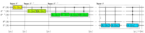
Figure 1: The tree-like memory structure of the quantum circuits for preparing a quantum mass function.

After $n$ layers, the initial state $\ket{0}^{\otimes n}$ transforms to $\ket{m}$ in Eq.(9). However, the method has the disadvantage of its exponential computational complexity $\mathcal{O}(n2^{n})$, which requires further speedup for real application scenarios.

III Operate Mass Function on Quantum Circuits

III-A Introduce Boolean Values to DST and Quantum States

From a new perspective of Boolean values, we reconsider the representation for focal sets in DST and quantum ground states. Further, the correspondence between DST and quantum computing is established through Boolean values.

III-A1 Boolean Values for Focal Set

Under an FoD of $n$ elements defined in Eq.(1), suppose $F$ is a focal set in the power set. $F$ can be determined by a series of Boolean values $i^{k},k=1,\dots,n$, where $i^{k}$ represents whether the element $\theta^{k}$ belongs to $F$. If it is true then $i^{k}$ is 1, otherwise it is 0.

$$i^{k}=\left\{\begin{array}[]{l}1,\quad\theta^{k}\in F\\ 0,\quad\theta^{k}\notin F\end{array}\right.,\quad k=1,\dots,n.$$ (10)

$F$ can be uniquely determined by these Boolean values $i^{n},\dots,i^{1}$. For convenient representation in decimal, the index number $i$ is introduced.

$$i=(i^{n}i^{n-1}\dots i^{1})_{2}=2^{n-1}i^{n}+2^{n-2}i^{n-1}+\dots+2^{0}i^{1}.$$ (11)

Since $i^{n},\dots,i^{1}$ are all Boolean values, the range of $i$ is from 0 to $2^{n}-1$. Therefore, for any element in the power set, unique corresponding Boolean values can be found along with a corresponding decimal index. So a mapping $\mathcal{F}$ can be created between the index and the elements in the power set.

$$\mathcal{F}:i=(i^{n}i^{n-1}\dots i^{1})_{2}\in\mathbb{Z}\rightarrow 2^{\Theta}.$$ (12)

For the case of $n=3$, the correspondence is shown in the following table II.

III-A2 Boolean Values for Quantum States

For a quantum system of $n$ qubits, it generates $2^{n}$ mutually orthogonal quantum ground states. They can be represented by $n$ Boolean values $\ket{i^{n}i^{n-1}\dots i^{1}}$, whose decimal representation is $\ket{i}_{D}$. Since Boolean values are mapped to focal sets, each quantum ground state corresponds to each focal set through the representation of Boolean values, which is presented in table II.

TABLE II: Correspondence between indexes, Boolean values, and focal sets under an FoD of 3 elements.

Index: $i$	0	1	2	3
Boolean value: $i^{3}i^{2}i^{1}$	000	001	010	011
Focal Set: $\mathcal{F}(i^{3}i^{2}i^{1})$	$\emptyset$	$\{\theta^{1}\}$	$\{\theta^{2}\}$	$\{\theta^{2}\theta^{1}\}$
Quantum State $\ket{i^{3}i^{2}i^{1}}$	$\ket{000}$	$\ket{001}$	$\ket{010}$	$\ket{011}$
Index: $i$	4	5	6	7
Boolean value: $i^{3}i^{2}i^{1}$	100	101	110	111
Focal set: $\mathcal{F}(i^{3}i^{2}i^{1})$	$\theta^{3}$	$\{\theta^{3}\theta^{1}\}$	$\{\theta^{3}\theta^{2}\}$	$\{\theta^{3}\theta^{2}\theta^{1}\}$
Quantum State $\ket{i^{3}i^{2}i^{1}}$	$\ket{100}$	$\ket{101}$	$\ket{110}$	$\ket{111}$

Thus the quantum mass function $\ket{m}$ defined in Eq.(9) is equivalent to the following Boolean form:

$$\ket{m}=\sum_{i^{n}=0}^{1}\dots\sum_{i^{1}=0}^{1}\sqrt{m(\mathcal{F}(i^{n}\dots i^{1}))}\ket{i^{n}\dots i^{1}}$$ (13)

III-B Implement DST Operations on Quantum Circuits

Since Boolean values has been introduced for focal sets, the Boolean algebraic form of DST operations can be derived including the negation of mass function and multiple rules of combination. Next, we hope to utilize quantum circuits to implement Boolean algebra to achieve DST operations.

III-B1 Boolean Algebra for DST Operations

The set operators involved in the definitions of DST operations, including complement $\bar{\quad}$, intersection $\cap$, and union $\cup$ in set theory, can be represented by Boolean algebra.

First, for the negation, the complement is involved in its definition in Eq.(4). Suggest that $F_{1}$ and $F_{2}$ are complementary sets of each other. For a single element $\theta^{k}$ in FoD, it either belongs to $F_{1}$ or its complement set $F_{2}$, which can derive that

$$F_{2}=\overline{F_{1}}\quad\Rightarrow\quad i_{2}^{k}=\neg i_{1}^{k};$$ (14)

where $i_{r}$ and $i_{r}^{k}$ denote the index and Boolean values for $F_{r}$, respectively. Therefore, the definition of the negation in Eq.(4) can be expressed with Boolean algebra:

$$\overline{m}(\mathcal{F}(i^{n}i^{n-1}\dots i^{1}))=m(\mathcal{F}(\neg i^{n}\neg i^{n-1}\dots\neg i^{1})).$$ (15)

Besides, the intersection and union in set theory can be transformed into the form of Boolean algebra with AND operator $\land$ and OR operator $\vee$.

$$F=F_{1}\cap F_{2}\cap\dots\cap F_{p}\quad\Rightarrow\quad i^{k}=i_{1}^{k}\land i^{k}_{2}\land\dots\land i^{k}_{p};$$ (16)

$$F=F_{1}\cup F_{2}\cup\dots\cup F_{p}\quad\Rightarrow\quad i^{k}=i_{1}^{k}\vee i^{k}_{2}\vee\dots\vee i^{k}_{p}.$$ (17)

Similarly, since CRC and DRC respectively utilize the intersection and union operations, one can obtain the variation of the definitions Eq.(5) and (6) with Boolean algebra.

$$m(\mathcal{F}(i^{n}\dots i^{1})) =\sum_{i_{1}^{n}\land\dots\land i_{p}^{n}=i^{n}}\dots\sum_{i_{1}^{1}\land\dots\land i_{p}^{1}=i^{1}}$$ (18)

$$\prod_{r=1}^{p}m_{r}(\mathcal{F}(i_{r}^{n}\dots i_{r}^{1})),\quad m=m_{1}\hbox{ \leavevmode\hbox to8.17pt{\vbox to9.44pt{\text{[drawing]}}}}\dots\hbox{ \leavevmode\hbox to8.17pt{\vbox to9.44pt{\text{[drawing]}}}}m_{p}; \cap \cap \cap \cap$$

$$m(\mathcal{F}(i^{n}\dots i^{1})) =\sum_{i_{1}^{n}\vee\dots\vee i_{p}^{n}=i^{n}}\dots\sum_{i_{1}^{1}\vee\dots\vee i_{p}^{1}=i^{1}}$$ (19)

$$\prod_{r=1}^{p}m_{r}(\mathcal{F}(i_{r}^{n}\dots i_{r}^{1})),\quad m=m_{1}\hbox{ \leavevmode\hbox to8.17pt{\vbox to9.44pt{\text{[drawing]}}}}\dots\hbox{ \leavevmode\hbox to8.17pt{\vbox to9.44pt{\text{[drawing]}}}}m_{p}. \cup \cup \cup \cup$$

Compared to the original definition, the involved set operations $F_{1}\cap\dots\cap F_{p}=F$ and $F_{1}\cup\dots\cup F_{p}=F$ are replaced by $n$ summation operations that are bounded by the Boolean algebra. One can extend the basic Boolean operators (NOT, AND, OR) to derive Boolean algebraic forms of more complex set-theoretic definitions e.g. the exclusive disjunctive rule in Eq.(7) and the customized rule in Eq.(8).

$$m(\mathcal{F}(i^{n}\dots i^{1}))=\sum_{(i_{1}^{n}\land\neg i_{2}^{n})\vee(\neg i_{1}^{n}\land i_{2}^{n})=i^{n}}\dots\sum_{(i_{1}^{1}\land\neg i_{2}^{1})\vee(\neg i_{1}^{1}\land i_{2}^{1})=i^{1}}$$ (20)

$$\prod_{j=1}^{2}m_{r}(\mathcal{F}(i_{r}^{n}\dots i_{r}^{1})),\quad m=m_{1}\hbox{ \leavevmode\hbox to9.4pt{\vbox to12.34pt{\text{[drawing]}}}}m_{2} \underline{\cup} \underline{\cup}$$ ;

$$m(\mathcal{F}(i^{n}\dots i^{1}))=\sum_{(\neg(i_{1}^{n}\land i_{2}^{n}))\land(i_{2}^{n}\vee i_{3}^{n})=i^{n}}\dots\sum_{(\neg(i_{1}^{1}\land i_{2}^{1}))\land(i_{2}^{1}\vee i_{3}^{1})=i^{1}}$$ (21)

$$\prod_{r=1}^{3}m_{r}(\mathcal{F}(i_{r}^{n}\dots i_{r}^{1})),\quad m=(\overline{m_{1}\hbox{ \leavevmode\hbox to9.4pt{\vbox to10.55pt{\text{[drawing]}}}}m_{2}})\hbox{ \leavevmode\hbox to9.4pt{\vbox to10.55pt{\text{[drawing]}}}}(m_{2}\hbox{ \leavevmode\hbox to9.4pt{\vbox to10.55pt{\text{[drawing]}}}}m_{3}) {\cap} {\cap} {\cup} {\cap} {\cap} {\cup}$$ .

III-B2 Negation of a Mass Function on Quantum Circuits

The Boolean algebraic form of the negation of a mass function is expressed in Eq.(15), where each Boolean value should satisfy NOT operation in Eq.(14). Since the Pauli-$X$ gate is the quantum equivalent of the classical NOT gate, mapping $\ket{0}$ to $\ket{1}$ and $\ket{1}$ to $\ket{0}$, Eq.(14) can be realized by applying one $X$ gate on the corresponding qubit to convert $\ket{i^{k}}$ to $\ket{\neg i^{k}}$. Thus with the quantum mass function, the quantum version of the negation in Eq.(15) can be represented on quantum circuits by applying $n$ Pauli-$X$ gates on each qubit after preparing $\ket{m}$. The quantum circuit is shown in Fig.2.

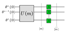
Figure 2: The quantum circuit for negation.

After $X$ gates, the original quantum mass function $\ket{m}$ in Eq.(13) becomes the state $\ket{\overline{m}}$, which represents the quantum mass function of $\overline{m}$. The proof is as follows.

$$\ket{\psi} =\sum_{i^{n}=0}^{1}\dots\sum_{i^{1}=0}^{1}\sqrt{m(\mathcal{F}(i^{n}\dots i^{1}))}\ket{\neg i^{n}\dots\neg i^{1}}$$ (22)

$$=\sum_{i^{n}=0}^{1}\dots\sum_{i^{1}=0}^{1}\sqrt{m(\mathcal{F}(\neg i^{n}\dots\neg i^{1}))}\ket{i^{n}\dots i^{1}}=\ket{\overline{m}}.$$

III-B3 CRC on Quantum Circuits

Consistent with the case of negation, to achieve the Boolean algebraic form of CRC in Eq.(18), Boolean values are required to satisfy the restriction of conjunction in Eq.(16). The conjunction suggests that the result is 1 only if all Boolean values are 1, otherwise, it is 0. Actually, in quantum mass functions, one can pick one of the superpositions with all $\ket{1}$ by using the CNOT gate and setting all the qubits associated with these Boolean values as the control qubits. In this case, the target qubit flips only if control qubits are all in the state $\ket{1}$. Based on the idea, the quantum circuit displayed in Fig.3(a) is designed to realize CRC for $p$ different mass functions.

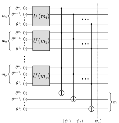
(a) CRC

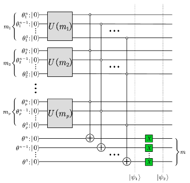
(b) DRC

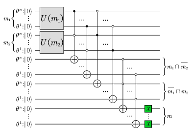
(c) Exclusive disjunctive

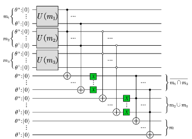
(d) Customized

Figure 3: Quantum circuits for multiple rules of combination.

The first step is preparing the initial quantum mass function for $m_{1},\dots,m_{p}$ respectively. Second, the conjunction in Eq.(16) is realized by utilizing CNOT gate element by element from $\theta^{n}$ to $\theta^{1}$. After $n$ CNOT operations, the final state can be expressed in Eq.(23). The state is be mathematically proven in Appendix 1.

$$\ket{\psi_{n}} =\sum_{j^{n}=0}^{1}\dots\sum_{j^{1}=0}^{1}\Bigg{\{}\sum_{i_{1}^{n}\wedge\dots\wedge i_{p}^{n}=j^{n}}\dots\sum_{i_{1}^{1}\wedge\dots\wedge i_{p}^{1}=j^{1}}$$ (23)

$$\prod_{r=1}^{p}\sqrt{m_{r}(\mathcal{F}(i_{r}^{n}\dots i_{r}^{1}))}\bigotimes_{r=1}^{p}\ket{i_{r}^{n}\dots i_{r}^{1}}\ket{j^{n}\dots j^{1}}\Bigg{\}}.$$

Due to the orthogonality of ground states, the amplitude $A$ of the superposition $\ket{j^{n}\dots j^{1}}$ for the last $n$ qubits can be extracted as displayed below.

$$A(\ket{j^{n}j^{n-1}\dots j^{1}})$$ (24)

$$=\sqrt{\sum_{i_{1}^{n}\wedge\dots\wedge i_{p}^{n}=j^{n}}\dots\sum_{i_{1}^{1}\wedge\dots\wedge i_{p}^{1}=j^{1}}\prod_{r=1}^{p}m_{r}(\mathcal{F}(i_{r}^{n}\dots i_{r}^{1}))}$$

$$=\sqrt{m(\mathcal{F}(j^{n}\dots j^{1}))},\quad m=m_{1}\hbox{ \leavevmode\hbox to8.17pt{\vbox to9.44pt{\text{[drawing]}}}}\dots\hbox{ \leavevmode\hbox to8.17pt{\vbox to9.44pt{\text{[drawing]}}}}m_{p}. \cap \cap \cap \cap$$

And the amplitude exactly corresponds to the square root value of the combined mass function defined in Eq.(18). Thus, in terms of the amplitude, the final state can be the quantum mass function after combining by CRC. Compared to the quantum mass function constructed by the tree-like memory structure in Section 3.2, the only difference is that this state is entangled with other parts in quantum circuits.

In order to convert it to the classical version, one can measure the last $n$ qubits and record the probability $P(j^{n}j^{n-1}\dots j^{1})$, which is equal to the mass after CRC.

$$P(j^{n}j^{n-1}\dots j^{1})=|A(\ket{j^{n}j^{n-1}\dots j^{1}})|^{2}$$ (25)

$$=m(\mathcal{F}(j^{n}j^{n-1}\dots j^{1})),\quad m=m_{1}\hbox{ \leavevmode\hbox to8.17pt{\vbox to9.44pt{\text{[drawing]}}}}\dots\hbox{ \leavevmode\hbox to8.17pt{\vbox to9.44pt{\text{[drawing]}}}}m_{p}. \cap \cap \cap \cap$$

III-B4 DRC on Quantum Circuits

Similar to the conjunctive rule, one has to represent the disjunction in Eq.(17) on quantum circuits to achieve the Boolean algebraic form of DRC expressed in Eq.(19). Since disjunction cannot be obviously represented by quantum gates whereas quantum circuits have been proposed to realize negation and conjunction in previous sections, we consider utilizing De Morgan’s laws to replace the disjunctive regulation in Eq.(17) by combining negation and conjunction.

$$i^{k}=i_{1}^{k}\vee i^{k}_{2}\vee\dots\vee i^{k}_{p}\Rightarrow i^{k}=\neg(\neg i_{1}^{k}\wedge\neg i^{k}_{2}\wedge\dots\wedge\neg i^{k}_{p})$$ (26)

According to Eq.(26), DRC can be implemented in two steps. First, use CNOT gates to achieve $\neg i_{1}^{k}\wedge\neg i^{k}_{2}\wedge\dots\wedge\neg i^{k}_{p}$, which utilize similar quantum circuits for CRC. But in this case, the target qubit is set to flip when all control qubits are $\ket{1}$ instead of $\ket{0}$ because NOT applies before AND for each Boolean value. The control position is represented by a hollow point in the diagram. Second, achieve the NOT operations by implementing $X$ gates, with the same quantum circuits for negation. Therefore, by combining the two steps, the quantum circuits for DRC are displayed in Fig.3(b).

According to the proof displayed in Appendix 2, the final state $\ket{\psi_{2}}$ is:

$$\ket{\psi_{2}} =\sum_{j^{n}=0}^{1}\dots\sum_{j^{1}=0}^{1}\Bigg{\{}\sum_{i_{1}^{n}\vee\dots\vee i_{p}^{n}=j^{n}}\dots\sum_{i_{1}^{1}\vee\dots\vee i_{p}^{1}=j^{1}}$$ (27)

$$\quad\quad\prod_{r=1}^{p}\sqrt{m_{r}(\mathcal{F}(i_{r}^{n}\dots i_{r}^{1}))}\bigotimes_{r=1}^{p}\ket{i_{r}^{n}\dots i_{r}^{1}}\ket{j^{n}\dots j^{1}}\Bigg{\}}.$$

Similar to Eq.(24)(25), the final $n$ qubits contain the quantum mass function after DRC, which can be directly obtained by measurement probability.

$$P(j^{n}j^{n-1}\dots j^{1})=|A(\ket{j^{n}j^{n-1}\dots j^{1}})|^{2}$$ (28)

$$=m(\mathcal{F}(j^{n}j^{n-1}\dots j^{1})),\quad m=m_{1}\hbox{ \leavevmode\hbox to8.17pt{\vbox to9.44pt{\text{[drawing]}}}}\dots\hbox{ \leavevmode\hbox to8.17pt{\vbox to9.44pt{\text{[drawing]}}}}m_{p}. \cup \cup \cup \cup$$

III-B5 Extend to Other General Rules

In fact, the construction mentioned above of quantum circuits can be extended to realize any rules of combination derived from set-theoretic definitions. The steps can be summarized in the following three steps.

• Step 1: Transform the original definition of rules of combination into a Boolean algebraic version based on Boolean values for focal sets.

• Step 2: Analyze the Boolean values for each element of the FoD individually to obtain the constraints of Boolean algebra, which can be represented by the combination of three basic operators NOT, AND, OR.

• Step 3: For the derived Boolean algebraic constraints, decompose it into multiple stages, each of which involves only one basic Boolean operator. The circuit structure construction method for implementing the basic Boolean operators is displayed below.

  • NOT $\neg$: Use $X$ gate to flip every qubit.

  • AND $\land$: Group the qubits according to their corresponding elements, and operate each group by CNOT gate. Set the qubits in the group as control qubits, and introduce a new qubit as the target qubit. If a Boolean value is operated by NOT operation before the AND operation, the flip is applied when the corresponding control qubit is $\ket{0}$ instead of $\ket{1}$.

  • OR $\vee$: Utilize De Morgan’s laws to convert OR operation into the operation of NOT, AND that can be implemented on quantum circuits.

According to the proposed method, one can construct the quantum circuits for every stage and combine all the stages to form the final quantum circuits.

Below, we give specific examples of implementing exclusive disjunction and the customized rules of combination to explore the process to transform any of the set-theoretically based rules of combination into a quantum circuit implementation by the proposed three-step approach.

The exclusive disjunction rule of combination is originally defined in Eq.(7). In Step 1, the Boolean algebraic form has been obtained and expressed in Eq.(20). Then the corresponding Boolean constraints in Step 2 can be derived:

$$(i_{1}^{k}\land\neg i_{2}^{k})\vee(\neg i_{1}^{k}\land i_{2}^{k})=i^{k},\quad k=1,\dots,n.$$ (29)

In Step 3, according to the logical order, the above constraints can be divided into three stages: (1) AND: get $i_{1}^{k}\land\neg i_{2}^{k}$; (2) AND: get $\neg i_{1}^{k}\land i_{2}^{k}$; (3) OR: finally get $(i_{1}^{k}\land\neg i_{2}^{k})\vee(\neg i_{1}^{k}\land i_{2}^{k})$. Since each stage only contains one basic Boolean operation, one can construct the quantum circuits stage by stage following the method in Step 3. The final quantum circuit structure for implementing the exclusive disjunctive rule of combination is shown in Fig.3(c).

For the rule of combination customized by our own, in Step 1 the set-theoretical definition in Eq.(8) can be transformed into the Boolean algebraic version expressed in Eq.(21). In Step 2, by analyzing each element in FoD alone, a series of constraints on the Boolean algebra is generated as below.

$$(\neg(i_{1}^{k}\land i_{2}^{k}))\land(i_{2}^{k}\vee i_{3}^{k})=i^{k},\quad k=1,\dots,n.$$ (30)

In Step 3, quantum circuits can be constructed by dividing the constraint into the following implementation stages: (1) AND: get $i_{1}^{k}\land i_{2}^{k}$; (2) NOT: get $\neg(i_{1}^{k}\land i_{2}^{k})$; (3) OR: get $i_{2}^{k}\vee i_{3}^{k}$; (4) AND: finally get $(\neg(i_{1}^{k}\land i_{2}^{k}))\land(i_{2}^{k}\vee i_{3}^{k})$. Each implementation stage only involves one basic Boolean operator that corresponds to the structure of the circuit. Combining these stages of the circuit creates the quantum circuits for implementing the customized rule of combination, which is shown in Fig.3(d).

III-C Simulation

To prove that the various rules of combination can be implemented on quantum circuits with the proposed method, we simulate CRC, DRC, the exclusive disjunctive, and also the customized rules of combination in this section. Simulation is conducted on the Qiskit platform.

Given three mass function $m_{1},m_{2},m_{3}$ under an FoD of $A$ and $B$. For each focal set $\emptyset,A,B,AB$, the mass value is set as $m_{1}=[0.1,0.2,0.5,0.2]$, $m_{2}=[0.05,0.45,0.25,0.25]$, $m_{3}=[0.3,0.1,0.1,0.5]$. According to the quantum circuits displayed in Fig.3(a)-3(d), we respectively construct the quantum circuit for the rules of combination including (1) CRC to obtain $m_{1}\hbox{ \leavevmode\hbox to8.17pt{\vbox to9.44pt{\text{[drawing]}}}}m_{2}\hbox{ \leavevmode\hbox to8.17pt{\vbox to9.44pt{\text{[drawing]}}}}m_{3}$, (2) DRC to obtain $m_{1}\hbox{ \leavevmode\hbox to8.17pt{\vbox to9.44pt{\text{[drawing]}}}}m_{2}\hbox{ \leavevmode\hbox to8.17pt{\vbox to9.44pt{\text{[drawing]}}}}m_{3}$, (3) the exclusive disjunctive rule to obtain $m_{1}\hbox{ \leavevmode\hbox to9.4pt{\vbox to12.34pt{\text{[drawing]}}}}m_{2}$, (4) the customized rule to obtain $(\overline{m_{1}\hbox{ \leavevmode\hbox to9.4pt{\vbox to10.55pt{\text{[drawing]}}}}m_{2}})\hbox{ \leavevmode\hbox to9.4pt{\vbox to10.55pt{\text{[drawing]}}}}(m_{2}\hbox{ \leavevmode\hbox to9.4pt{\vbox to10.55pt{\text{[drawing]}}}}m_{3})$. As our method suggests, one can directly get the combined mass value by conducting measurements (1024 shots) and calculating the probability for every ground state. The quantum circuits and the simulation result are shown in Fig.4-7.

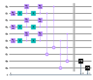
(a) Quantum circuit

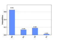
(b) Probability results

Figure 4: Simulation for CRC.

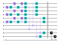
(a) Quantum circuit

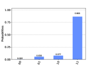
(b) Probability results

Figure 5: Simulation for DRC.

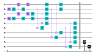
(a) Quantum circuit

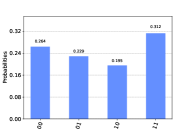
(b) Probability results

Figure 6: Simulation for the exclusive disjunctive rule of combination.

(a) Quantum circuit

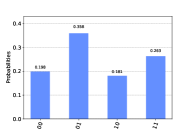
(b) Probability results

Figure 7: Simulation for the customized rule of combination.

TABLE III: The summary of results in the simulation and the comparison with the actual mass for four different rules of combination.

Focal set	Conjunctive			Disjunctive
	Simulated	Actual	Error	Simulated	Actual	Error
$\emptyset$	0.651	0.647	0.004	0.002	0.0015	0.0005
$A$	0.140	0.143	-0.003	0.056	0.0585	-0.0025
$B$	0.184	0.185	-0.001	0.077	0.0705	0.0065
$AB$	0.025	0.025	0	0.865	0.8695	-0.0045
Focal set	Exclusive disjunctive			Customized
	Simulated	Actual	Error	Simulated	Actual	Error
$\emptyset$	0.264	0.27	-0.006	0.198	0.207	-0.009
$A$	0.229	0.23	-0.001	0.358	0.343	0.015
$B$	0.195	0.19	0.005	0.181	0.193	-0.012
$AB$	0.312	0.31	0.002	0.263	0.257	0.006

To verify the feasibility of the method, in table III the simulated result is compared to the value of the actual combined mass functions, which are directly calculated by the set-theoretic definitions in Eq.(5-8). From the table data, the results obtained by measurement match the actual values. Certain errors encountered in the simulation are reasonable due to the limited number of shots (here is 1024) when measuring. One can increase the number of shots to extract more accurate amplitude information for qubits thus reducing the error.

IV Attribute Fusion-based Evidential Classifier

As the proposed quantum circuits structure suggests, the computation of implementing the combination rule has been exponentially accelerated on quantum circuits, where the complexity is $\mathcal{O}(n)$ under an FoD of $n$ elements. Thus, we introduced this efficient quantum circuit structure into the procedure of the classical classification method [50] to construct an evidential classifier on quantum circuits.

Assume that the data set be divided into $n$ classes denoting $\theta^{i},i=1,\dots,n$, which compose a FoD: $\Theta=\{\theta^{1},\dots,\theta^{n}\}$. All the data have $m$ attributes noted as $j=1,\dots,m$. Take the classic Iris data set as an example. The classes are Setosa ($\theta^{1}$), Versicolour ($\theta^{2}$), and Virginica ($\theta^{3}$) and the attributes are Sepal Length ($j=1$), Sepal Width ($j=2$), Petal Length ($j=3$), Petal Width ($j=4$), respectively. The evidential classifier consists of several components, which are discussed in detail below.

IV-A Procedure

IV-A1 Establish Gaussian Mixture Model (GMM)

GMM is a model of the sum of multiple Gaussian distributions, which is rich enough to fit any non-Gaussian probability distribution function for a variable [53]. GMM’s function expression is given by:

$$f(x) =\sum_{k=1}^{N}w_{k}N(x|\mu_{k},\sigma_{k})$$ (31)

$$=\sum_{k=1}^{N}w_{k}\frac{1}{\sqrt{2\pi\sigma_{k}^{2}}}\exp\left(-\frac{(x-\mu_{k})^{2}}{2\sigma_{k}^{2}}\right),$$

where $f(x)$ contains $N$ Gaussian components. $\mu_{k}$ and $\sigma_{k}$ are the mean and variance of each component. $w_{k}$ represents the weight associated with each component, satisfying $\sum_{k=1}^{N}w_{k}=1$.

A portion of the whole dataset is extracted as the training set to derive GMM’s function $f_{j}^{i}(x)$ for each attribute $j$ and class $\theta^{i}$. Thus there are $m\times n$ independent GMM to be established. To determine the parameters $w_{k},\mu_{k},\sigma_{k}$ in GMM, we utilize Expectation-maximization (EM) algorithm, which is summarized in the following steps. Suppose the input data is noted as $x_{l}$ where $l=1,\dots,L$.

1. Initialization of parameters: $w_{k},\mu_{k},\sigma_{k}$, where $k=1,\dots,N$.

2. E-step: Implement pseudo-posterior estimation. With the current model parameters, calculate the probability of considering $x_{l}$ to belong to $k$-th component.

   $$\gamma_{lk}=\frac{w_{k}N(x_{l}|\mu_{k},\sigma_{k})}{\sum_{r=1}^{N}w_{r}N(x_{l}|\mu_{r},\sigma_{r})}.$$ (32)

3. M-step: Re-estimate model parameters with the Maximum Likelihood Estimation (MLE). The updated parameters $w_{k}^{\prime},\mu_{k}^{\prime},\sigma_{k}^{\prime}$ can be determined by:

   $$w_{k}^{\prime} =\frac{1}{L}\sum_{l=1}^{L}\gamma_{lk};$$ (33)

   $$\mu_{k}^{\prime} =\frac{\sum_{l=1}^{L}\gamma_{lk}x_{l}}{\sum_{l=1}^{L}\gamma_{lk}};$$

   $$\sigma_{k}^{\prime} =\frac{\sum_{l=1}^{L}\gamma_{lk}(x_{l}-\mu_{k})^{2}}{\sum_{l=1}^{L}\gamma_{lk}}.$$

4. Loop E-step and M-step until parameters converge.

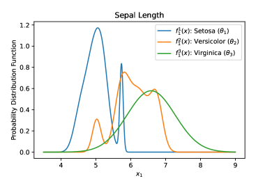
(a) Sepal Length ($j=1$)

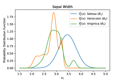
(b) Sepal Width ($j=2$)

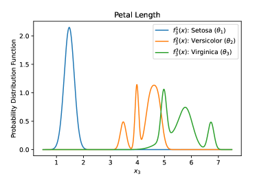
(c) Petal Length ($j=3$)

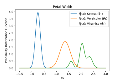
(d) Petal Width ($j=4$)

Figure 8: GMM for Iris data set.

For the example of the Iris data set, $3\times 4=12$ GMM should be established by EM algorithm for every attribute and class. Set the number of GMM components as $N=4$ the established GMM is shown in Fig.8.

IV-A2 Generate Mass Function

After the training stage of GMM, in the classification stage, each attribute $j$ of the input data can be evaluated by the GMM model and obtain the probability density $f_{j}^{i}(x_{j})$ for each class $\theta^{i}$. Then, we transform the probability density to Possibility Mass Function (PossMF) by normalization:

$$\pi_{1j}^{i}=\frac{f_{j}^{i}(x_{j})}{\max_{k}\left\{f_{j}^{k}(x_{j})\right\}},\quad\pi_{0j}^{i}=1-\pi_{1i}^{j},$$ (34)

where $\pi_{1j}^{i}$ and $\pi_{0j}^{i}$ represent the probability of supporting and not supporting class $\theta^{j}$ respectively.

Next, to handle the uncertainty in DST framework, a mass function is required to be generated according to PossMF. If the mass function is generated arbitrarily, one needs to use the tree-memory structure in Fig.1 to prepare the quantum mass function in Eq.(9). However, the preparing method involves exponential computational complexity $\mathcal{O}(n2^{n})$, which invalidates computational advantage in the application. To implement with lower complexity, we utilize a special method CD-BFT [54] to generate mass function, which is given by:

$$m_{j}(\mathcal{F}(i^{n}\dots i^{1}))=\prod_{k=1}^{n}\pi_{i^{k}j}^{k},\quad j=1,\dots,m.$$ (35)

CD-BFT is advantageous in information modeling and guarantees the combination rule consistency between possibilistic and evidential information. With the special mass structure generated by CD-BFT, one can use simpler structured quantum circuits as shown in Fig.9.

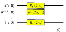
Figure 9: Simple structure quantum circuits.

According to the circuits, $R_{Y}$ gates are only applied for $n$ times independently without entanglement introduced. And the rotation angle $\alpha_{k}$ can be directly determined by PossMF:

$$\alpha_{k}=\arctan\left(\sqrt{\pi_{1j}^{k}/\pi_{0j}^{k}}\right).$$ (36)

The step is presented in Fig.11. Take the Iris data set as an example. Suppose the input data $x=[6.3,3.3,4.7,1.6]$, where each value corresponds to an attribute. Analyze the attribute Petal Length ($j=3$), whose GMM functions are presented in Fig.8. Since the attribute value $x_{3}=4.7$, according to Fig.8, the probability density is $f_{3}^{1}(x_{3})=0.0000$, $f_{3}^{2}(x_{3})=1.1000$, $f_{3}^{3}(x_{3})=0.1245$. After normalization PossMF is obtained: $\pi_{13}^{1}=0.0000,\pi_{03}^{1}=1.0000$; $\pi_{13}^{2}=1.0000,\pi_{03}^{2}=0.0000$;$\pi_{13}^{2}=0.1132,\pi_{03}^{2}=0.8868$. Finally, as Eq.(36) suggests, the angles can be determined: $\alpha_{1}=0$, $\alpha_{2}=\pi/2$, $\alpha_{3}=0.3431$.

IV-A3 Evidence Combination and Decision Making

As presented in Fig.11, the generated quantum mass functions for all attributes are fused together by CRC to achieve attribute fusion, which is given by: $m=m_{1}\hbox{ \leavevmode\hbox to8.17pt{\vbox to9.44pt{\text{[drawing]}}}}\dots\hbox{ \leavevmode\hbox to8.17pt{\vbox to9.44pt{\text{[drawing]}}}}m_{m}$. Here we utilize the proposed quantum algorithm of CRC for efficient implementation. Then the combined evidence $m$ is extracted from quantum states through measurement.

To make the decision, the final step is to convert $m$ to the probability representation $BetP$, which is implemented by:

$$BetP(\theta^{i})=\sum_{\theta_{i}\in F}\frac{1}{1-m(\emptyset)}\cdot\frac{m(F)}{|F|},$$ (37)

where $|\cdot|$ denotes the number of elements contained in the focal set. Then, the final decision is $\arg\max_{\theta^{i}}BetP(\theta^{i})$.

For the numeral example $x=[6.3,3.3,4.7,1.6]$, after evidence combination $m$ is obtained: $m(\theta^{2})=0.6725$ and $m(\theta^{3}\theta^{2})=0.3275$. According to Eq.(37), the transformed probability is: $BetP(\theta^{1})=0$, $BetP(\theta^{2})=0.8362$, $BetP(\theta^{3})=0.1638$. Therefore, the final classification decision is that the sample belongs to the class $\theta^{2}$.

The entire procedure of the attribute fusion-based evidential classifier is shown in Fig.11, where the quantum computer gets involved in the steps enclosed in the blue box with the quantum circuits as presented in Fig.11.

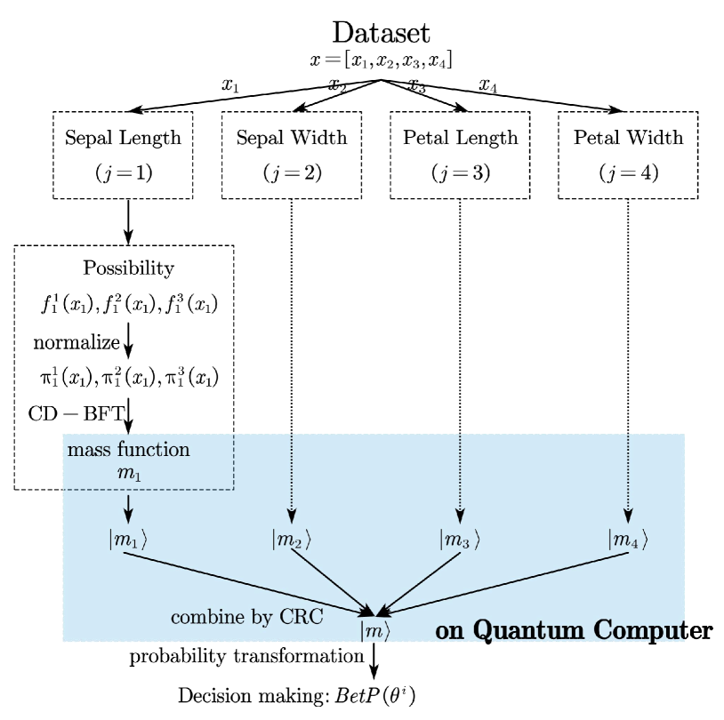
Figure 10: Flowchart for proposed attribute fusion-based evidential classifier (use Iris dataset as an example).

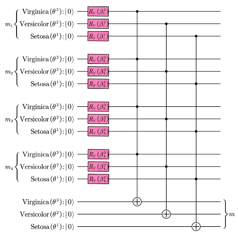
Figure 11: The quantum circuits for implementing evidence combinations involved in the evidential classifier. (use Iris dataset as an example).

IV-B Time Complexity Analysis

According to Fig.11, the proposed improvements over previous algorithms are the quantum implementation of classical CRC enclosed in the blue box. On quantum computers, the procedure involves Part I: generating quantum mass functions from the classical PossMF, and Part II: fusing evidence on quantum circuits. The time complexity required for previous algorithms is summarized in table IV.

TABLE IV: A comparison of time complexity.

Classical [50]	$\mathcal{O}(m4^{n})$
Quantum	Part I	Part II
	Tree-like Memory [41]: $\mathcal{O}(mn2^{n})$	HHL [41]: $\mathcal{O}(m\log(2^{n+1})2^{2n}/\varepsilon)$
		VQLS [33]: $\mathcal{O}(m\cdot poly(2^{n})\log(1/\varepsilon))$
	Proposed: $\mathcal{O}(mn)$	Proposed: $\mathcal{O}(n)$

But with the proposed quantum circuit as suggested in Fig.11, Part I is implemented by the simple structure. By acting $mn$ single qubit $R_{Y}$ gates, $m$ classical mass functions generated by CD-BFT can be prepared on quantum circuits. In Part II, one can use $n$ CNOT gates to obtain the combined quantum mass function. Therefore, according to table IV, our evidential classifier achieves exponential acceleration compared to previous algorithms, reducing the total time complexity to linear: $\mathcal{O}(mn)$.

IV-C Testing on Real Data Set

To verify the feasibility of the proposed attribute fusion-based evidential classifier, it is tested on several real data sets [55] of different numbers of attributes and classes. Their detail is presented in table V.

TABLE V: Data Set description.

Data Set	Sample: $L$	Class: $n$	Attribute: $m$
Iris	150	3	4
Haberman	306	2	3
Wine	178	3	13
Seeds	210	3	7
HTRU2	17898	2	8
Diabetes	768	2	8

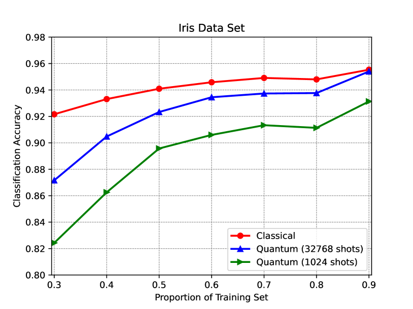
Figure 12: The classification accuracy for Iris data set.

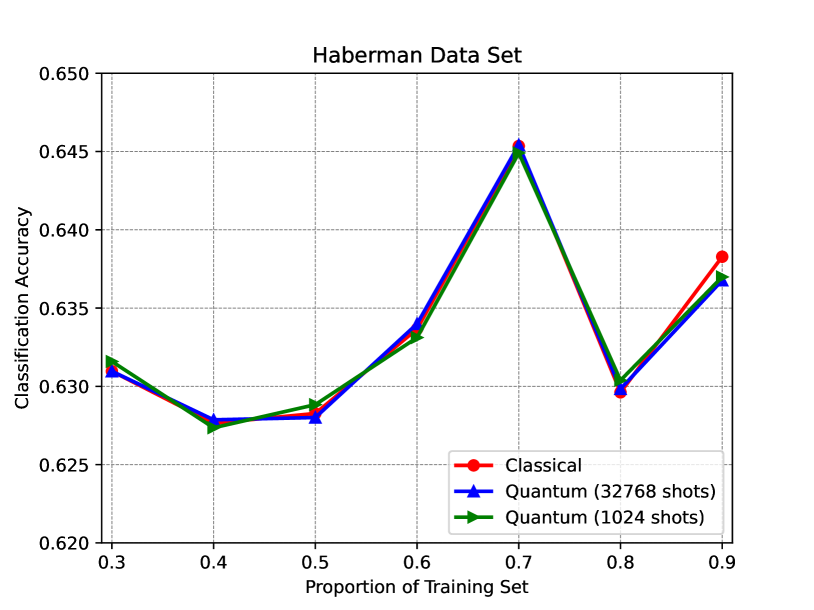
Figure 13: The classification accuracy for Haberman’s Survival data set.

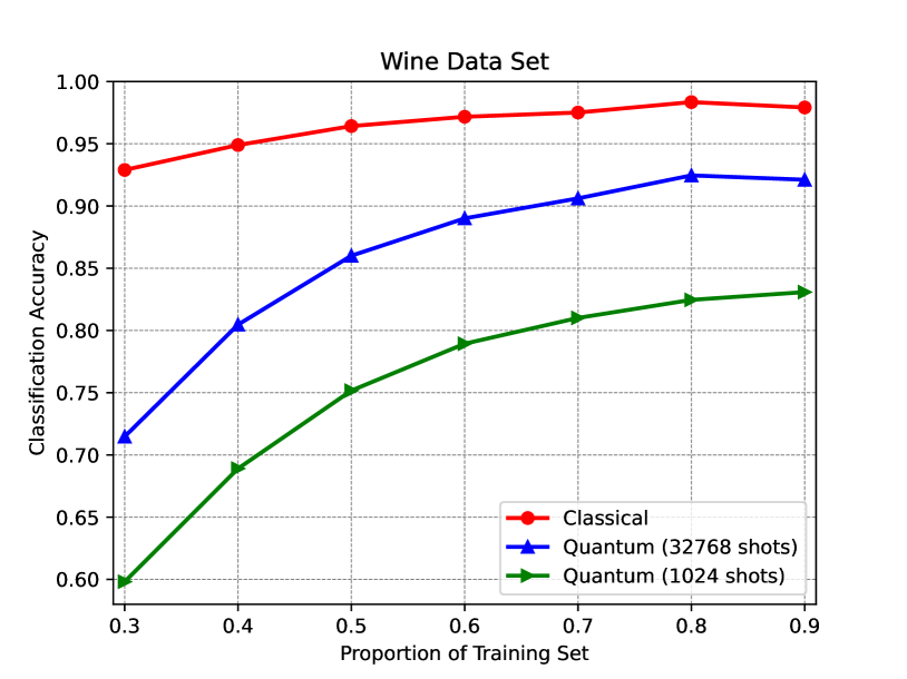
Figure 14: The classification accuracy for Wine data set.

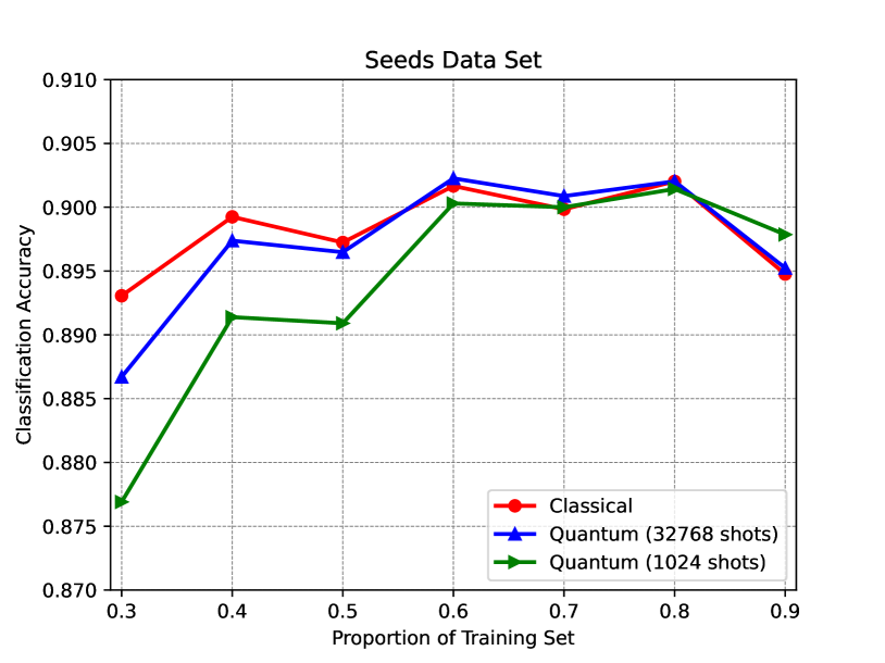
Figure 15: The classification accuracy for Seeds data set.

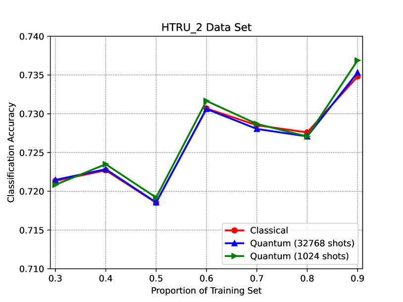
Figure 16: The classification accuracy for HTRU2 data set.

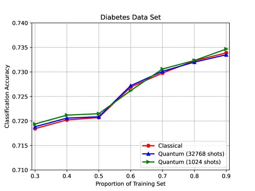
Figure 17: The classification accuracy for Diabetes data set.

The proportion of data assigned to the training sets is simulated from 0.3 to 0.9. GMM component is selected as 3. Under a certain proportion, we simulate the classical attribute classifier and the proposed quantum attribute classifier by conducting 100 independent experiments. The average accuracy is shown in Fig.17-17. Apart from the classical classifier (in red line), to demonstrate the effect of the number of shots measurement on accuracy, we select 1024 shots (in green line) and 32768 shots (in blue line) as examples. Simulation code has been uploaded to https://github.com/luohaooo/DST_Classifier_on_Quantum_Circuits.

Theoretically, the accuracy of the quantum method must be lower than that of the classical method because the proposed quantum method is based entirely on the classical model and the measurement of quantum systems brings error. And the measurement error can be eliminated by continually increasing the number of shots. However, according to the simulation results, only Iris and Wine data sets clearly demonstrate this result, especially in the case of low training proportion. As to other data sets, only a little difference in accuracy lies between classical and quantum methods, realizing ideal classification results.

V Conclusion

In this paper, we introduce Boolean values into the framework of DST and quantum computing and establish the correspondence between focal sets and quantum ground states. Then the set-theoretic definition of DST operations is reconsidered from a Boolean algebraic perspective. Based on that, a more flexible, efficient, and general quantum algorithm for implementing DST operations is proposed clarifying the essential link between DST and quantum computing mathematically and systematically. Simulations demonstrate the low error level of the algorithm. For the application of classification, we modify the preparation method of quantum mass functions and apply the proposed algorithm to complete the rule of combination for evidence from different attributes to obtain the attribute fusion-based evidential classifier on quantum circuits. Compared to the previous classical and quantum algorithms, the proposed classifier achieves exponential acceleration on time complexity. The final tests on real data sets verify the feasibility and accuracy of the classifier.

However, according to the proposed algorithm, the cost of reducing the time complexity is the linear increasing number of qubits required for the quantum system. Due to the current constraints on quantum resources in the current NISQ era, the practicality of this method will be limited. Therefore, reducing the size of the quantum system to design a spatially efficient method is an improvement direction.

For future work, since the paper demonstrates a unified framework mapping DST operations to quantum circuits, more applications in the DST field [48] can be accomplished on quantum circuits based on the proposed algorithm. From another point, the previous works focused on designing quantum circuits for accelerating DST operation. But it is time to break the limit since quantum states and operations have been given actual meaning by DST through the framework of Boolean algebra. Therefore, in the next step, we can innovate and implement the DST operations for handling uncertainty with the help of quantum computing. Further, DST brings interpretability to quantum systems, which encourages introducing DST to the current rapidly developing quantum machine learning algorithms [30, 31] and variational quantum algorithms [34, 33] to improve the performance.

[Proof of the Zonklar Equations] Use $\backslash$appendix if you have a single appendix: Do not use $\backslash$section anymore after $\backslash$appendix, only $\backslash$section*. If you have multiple appendixes use $\backslash$appendices then use $\backslash$section to start each appendix. You must declare a $\backslash$section before using any $\backslash$subsection or using $\backslash$label ($\backslash$appendices by itself starts a section numbered zero.)

Appendix A Proof of Implementing CRC on Quantum Circuits

According to Fig.3(a), the quantum system contains $(p+1)n$ qubits, including $p+1$ parts of quantum mass functions. The first $p$ parts represent $\ket{m_{1}},\dots,\ket{m_{p}}$. And the initial state of last $n$ qubits is $\ket{0}^{\otimes n}$. Thus the entire quantum state at the initial stage can be derived.

$$\ket{\psi_{0}} =\ket{m_{1}}\ket{m_{2}}\dots\ket{m_{p}}\ket{0}^{\otimes n}$$ (38)

$$=\sum_{i_{1}=0}^{2^{n}-1}\dots\sum_{i_{p}=0}^{2^{n}-1}\prod_{r=1}^{p}\sqrt{m_{r}(\mathcal{F}(i_{r}))}\bigotimes_{r=1}^{p}\ket{i_{r}}_{D}\ket{0}^{\otimes n}.$$

Here $i_{r}(r=1,\dots,p)$ is the decimal representation of the Boolean values satisfying $i_{r}=(i_{r}^{n}i_{r}^{n-1}\dots i_{r}^{1})_{2}$. Then the first CNOT gate is applied on qubits associated with $\theta^{n}$, flipping the target qubit to $\ket{1}$ when $i_{1}^{n}\wedge\dots i_{p}^{n}=1$. And the quantum state becomes:

$$\ket{\psi_{1}}=$$ (39)

$$\left\{\sum_{i_{1}^{n}\wedge\dots\wedge i_{p}^{n}=0}\left[\sum_{i_{1}=0}^{2^{n}-1}\dots\sum_{i_{p}=0}^{2^{n}-1}\prod_{r=1}^{p}\sqrt{m_{r}(\mathcal{F}(i_{r}))}\bigotimes_{r=1}^{p}\ket{i_{r}}_{D}\right]\ket{0}\right.$$

$$\left.+\sum_{i_{1}^{n}\wedge\dots\wedge i_{p}^{n}=1}\left[\sum_{i_{1}=0}^{2^{n}-1}\dots\sum_{i_{p}=0}^{2^{n}-1}\prod_{r=1}^{p}\sqrt{m_{r}(\mathcal{F}(i_{r}))}\bigotimes_{r=1}^{p}\ket{i_{r}}_{D}\right]\ket{1}\right\}$$

$$\ket{0}^{\otimes n-1}.$$

Similarly, after the $k$-th CNOT operation, the quantum state $\ket{\psi_{k}}$ can be deduced.

$$\ket{\psi_{k}}=$$ (40)

$$\sum_{j^{n}=0}^{1}\dots\sum_{j^{n-k+1}=0}^{1}\left\{\sum_{i_{1}^{n}\wedge\dots\wedge i_{p}^{n}=j^{n}}\dots\sum_{i_{1}^{n-k+1}\wedge\dots\wedge i_{p}^{n-k+1}=j^{n-k+1}}\right.$$

$$\left.\left[\sum_{i_{1}=0}^{2^{n}-1}\dots\sum_{i_{p}=0}^{2^{n}-1}\prod_{r=1}^{p}\sqrt{m_{r}(\mathcal{F}(i_{r}))}\bigotimes_{r=1}^{p}\ket{i_{r}}_{D}\right]\ket{j^{n}\dots j^{n-k+1}}\right\}$$

$$\ket{0}^{\otimes n-k}.$$

Therefore, according to Eq.(40), when $k=n$ the final quantum state is obtained.

$$\ket{\psi_{n}} =\sum_{j^{n}=0}^{1}\dots\sum_{j^{1}=0}^{1}\Bigg{\{}\sum_{i_{1}^{n}\wedge\dots\wedge i_{p}^{n}=j^{n}}\dots\sum_{i_{1}^{1}\wedge\dots\wedge i_{p}^{1}=j^{1}}\Bigg{[}\sum_{i_{1}=0}^{2^{n}-1}\dots\sum_{i_{p}=0}^{2^{n}-1}$$ (41)

$$\prod_{r=1}^{p}\sqrt{m_{r}(\mathcal{F}(i_{r}))}\bigotimes_{r=1}^{p}\ket{i_{r}}_{D}\Bigg{]}\ket{j^{n}\dots j^{1}}\Bigg{\}}$$

$$=\sum_{j^{n}=0}^{1}\dots\sum_{j^{1}=0}^{1}\Bigg{\{}\sum_{i_{1}^{n}\wedge\dots\wedge i_{p}^{n}=j^{n}}\dots\sum_{i_{1}^{1}\wedge\dots\wedge i_{p}^{1}=j^{1}}$$

$$\prod_{r=1}^{p}\sqrt{m_{r}(\mathcal{F}(i_{r}^{n}i_{r}^{n-1}\dots i_{r}^{1}))}\bigotimes_{r=1}^{p}\ket{i_{r}^{n}i_{r}^{n-1}\dots i_{r}^{1}}\ket{j^{n}\dots j^{1}}\Bigg{\}}.$$

Appendix B Proof of Implementing DRC on Quantum Circuits

According to Fig.3(b), in step 1, compared to the conjunctive rule, the method only takes the reverse of the input Boolean value. Therefore, according to Eq.(23), the quantum state $\ket{\psi_{1}}$ after step 1 can be derived.

$$\ket{\psi_{1}} =\sum_{j^{n}=0}^{1}\dots\sum_{j^{1}=0}^{1}\Bigg{\{}\sum_{\neg i_{1}^{n}\wedge\dots\wedge\neg i_{p}^{n}=j^{n}}\dots\sum_{\neg i_{1}^{1}\wedge\dots\wedge\neg i_{p}^{1}=j^{1}}$$ (42)

$$\prod_{r=1}^{p}\sqrt{m_{r}(\mathcal{F}(i_{r}^{n}\dots i_{r}^{1}))}\bigotimes_{r=1}^{p}\ket{i_{r}^{n}\dots i_{r}^{1}}\ket{j^{n}\dots j^{1}}\Bigg{\}}.$$

In step 2, $X$ gates are implemented on the last $n$ qubits, flipping the state $\ket{j^{n}\dots j^{1}}$. The quantum state $\ket{\psi_{2}}$ can be expressed and processed by Boolean algebra as follows.

$$\ket{\psi_{2}} =\sum_{j^{n}=0}^{1}\dots\sum_{j^{1}=0}^{1}\Bigg{\{}\sum_{\neg i_{1}^{n}\wedge\dots\wedge\neg i_{p}^{n}=j^{n}}\dots\sum_{\neg i_{1}^{1}\wedge\dots\wedge\neg i_{p}^{1}=j^{1}}$$ (43)

$$\quad\quad\prod_{r=1}^{p}\sqrt{m_{r}(\mathcal{F}(i_{r}^{n}\dots i_{r}^{1}))}\bigotimes_{r=1}^{p}\ket{i_{r}^{n}\dots i_{r}^{1}}\ket{\neg j^{n}\dots\neg j^{1}}\Bigg{\}}$$

$$=\sum_{j^{n}=0}^{1}\dots\sum_{j^{1}=0}^{1}\Bigg{\{}\sum_{\neg i_{1}^{n}\wedge\dots\wedge\neg i_{p}^{n}=\neg j^{n}}\dots\sum_{\neg i_{1}^{1}\wedge\dots\wedge\neg i_{p}^{1}=\neg j^{1}}$$

$$\quad\quad\prod_{r=1}^{p}\sqrt{m_{r}(\mathcal{F}(i_{r}^{n}\dots i_{r}^{1}))}\bigotimes_{r=1}^{p}\ket{i_{r}^{n}\dots i_{r}^{1}}\ket{j^{n}\dots j^{1}}\Bigg{\}}$$

$$=\sum_{j^{n}=0}^{1}\dots\sum_{j^{1}=0}^{1}\Bigg{\{}\sum_{i_{1}^{n}\vee\dots\vee i_{p}^{n}=j^{n}}\dots\sum_{i_{1}^{1}\vee\dots\vee i_{p}^{1}=j^{1}}$$

$$\quad\quad\prod_{r=1}^{p}\sqrt{m_{r}(\mathcal{F}(i_{r}^{n}\dots i_{r}^{1}))}\bigotimes_{r=1}^{p}\ket{i_{r}^{n}\dots i_{r}^{1}}\ket{j^{n}\dots j^{1}}\Bigg{\}}.$$

References

- [1] A. P. Dempster, “Upper and Lower Probabilities Induced by a Multivalued Mapping,” The Annals of Mathematical Statistics, vol. 38, no. 2, pp. 325–339, 1967.
- [2] G. Shafer, A mathematical theory of evidence. Princeton university press, 1976, vol. 42.
- [3] T. Denœux, “Conjunctive and disjunctive combination of belief functions induced by nondistinct bodies of evidence,” Artificial Intelligence, vol. 172, no. 2, pp. 234–264, 2008.
- [4] P. Smets, “The -junctions: Combination operators applicable to belief functions,” in Qualitative and Quantitative Practical Reasoning, D. M. Gabbay, R. Kruse, A. Nonnengart, and H. J. Ohlbach, Eds. Berlin, Heidelberg: Springer Berlin Heidelberg, 1997, pp. 131–153.
- [5] M. Zhou, X.-B. Liu, Y.-W. Chen, X.-F. Qian, J.-B. Yang, and J. Wu, “Assignment of attribute weights with belief distributions for madm under uncertainties,” Knowledge-Based Systems, vol. 189, p. 105110, 2020.
- [6] J.-B. Yang and D.-L. Xu, “Nonlinear information aggregation via evidential reasoning in multiattribute decision analysis under uncertainty,” IEEE Transactions on Systems, Man, and Cybernetics - Part A: Systems and Humans, vol. 32, no. 3, pp. 376–393, 2002.
- [7] C. Fu, M. Xue, W. Chang, D. Xu, and S. Yang, “An evidential reasoning approach based on risk attitude and criterion reliability,” Knowledge-Based Systems, vol. 199, p. 105947, 2020.
- [8] F. Xiao and W. Pedrycz, “Negation of the quantum mass function for multisource quantum information fusion with its application to pattern classification,” IEEE Transactions on Pattern Analysis and Machine Intelligence, p. DOI: 10.1109/TPAMI.2022.3167045, 2022.
- [9] F. Xiao, J. Wen, and W. Pedrycz, “Generalized divergence-based decision making method with an application to pattern classification,” IEEE Transactions on Knowledge and Data Engineering, 2022.
- [10] F. Xiao, Z. Cao, and C.-T. Lin, “A complex weighted discounting multisource information fusion with its application in pattern classification,” IEEE Transactions on Knowledge and Data Engineering, 2022.
- [11] X. Deng, S. Xue, and W. Jiang, “A novel quantum model of mass function for uncertain information fusion,” Information Fusion, vol. 89, pp. 619–631, 2023.
- [12] A. G. Bronevich and A. E. Lepskiy, “Measures of conflict, basic axioms and their application to the clusterization of a body of evidence,” Fuzzy Sets and Systems, vol. 446, pp. 277–300, 2022.
- [13] J.-B. Yang and D.-L. Xu, “Evidential reasoning rule for evidence combination,” Artificial Intelligence, vol. 205, pp. 1–29, 2013.
- [14] F. Xiao, “Generalization of Dempster–Shafer theory: A complex mass function,” Applied Intelligence, vol. 50, no. 10, pp. 3266–3275, 2020.
- [15] L. Pan and Y. Deng, “A new complex evidence theory,” Information Sciences, vol. 608, pp. 251–261, 2022.
- [16] J. A. Barnett, “Computational methods for a mathematical theory of evidence,” in Proceedings of the 7th International Joint Conference on Artificial Intelligence - Volume 2, ser. IJCAI’81. San Francisco, CA, USA: Morgan Kaufmann Publishers Inc., 1981, pp. 868–875.
- [17] B. Tessem, “Approximations for efficient computation in the theory of evidence,” Artificial Intelligence, vol. 61, no. 2, pp. 315–329, 1993.
- [18] N. Wilson, “A Monte-Carlo Algorithm for Dempster-Shafer Belief,” in Uncertainty Proceedings 1991, B. D. D’Ambrosio, P. Smets, and P. P. Bonissone, Eds. San Francisco (CA): Morgan Kaufmann, 1991, pp. 414–417.
- [19] M. Benalla, B. Achchab, and H. Hrimech, “On the computational complexity of Dempster’s Rule of combination, a parallel computing approach,” Journal of Computational Science, vol. 50, p. 101283, 2021.
- [20] M. A. Nielsen and I. Chuang, “Quantum computation and quantum information,” 2002.
- [21] P. W. Shor, “Polynomial-time algorithms for prime factorization and discrete logarithms on a quantum computer,” SIAM review, vol. 41, no. 2, pp. 303–332, 1999.
- [22] L. K. Grover, “A fast quantum mechanical algorithm for database search,” in Proceedings of the twenty-eighth annual ACM symposium on Theory of computing, 1996, pp. 212–219.
- [23] S.-T. Cheng and C.-Y. Wang, “Quantum switching and quantum merge sorting,” IEEE Transactions on Circuits and Systems I: Regular Papers, vol. 53, no. 2, pp. 316–325, 2006.
- [24] Y.-L. Ju, I.-M. Tsai, and S.-Y. Kuo, “Quantum circuit design and analysis for database search applications,” IEEE Transactions on Circuits and Systems I: Regular Papers, vol. 54, no. 11, pp. 2552–2563, 2007.
- [25] I.-A. Fyrigos, V. Ntinas, N. Vasileiadis, G. C. Sirakoulis, P. Dimitrakis, Y. Zhang, and I. G. Karafyllidis, “Memristor crossbar arrays performing quantum algorithms,” IEEE Transactions on Circuits and Systems I: Regular Papers, vol. 69, no. 2, pp. 552–563, 2022.
- [26] M. R. Laskar and A. K. Dutta, “A complexity-efficient quantum architecture and simulation for eigen spectrum estimation of vandermonde system in a large antenna array,” IEEE Transactions on Circuits and Systems I: Regular Papers, vol. 70, no. 5, pp. 2106–2119, 2023.
- [27] A. W. Harrow, A. Hassidim, and S. Lloyd, “Quantum algorithm for linear systems of equations,” Physical review letters, vol. 103, no. 15, p. 150502, 2009.
- [28] S. Lloyd, M. Mohseni, and P. Rebentrost, “Quantum principal component analysis,” Nature Physics, vol. 10, no. 9, pp. 631–633, 2014. [Online]. Available: https://doi.org/10.1038/nphys3029
- [29] P. Rebentrost, M. Mohseni, and S. Lloyd, “Quantum support vector machine for big data classification,” Phys. Rev. Lett., vol. 113, p. 130503, Sep 2014. [Online]. Available: https://link.aps.org/doi/10.1103/PhysRevLett.113.130503
- [30] J. Shi, W. Wang, X. Lou, S. Zhang, and X. Li, “Parameterized hamiltonian learning with quantum circuit,” IEEE Transactions on Pattern Analysis and Machine Intelligence, vol. 45, no. 5, pp. 6086–6095, 2023.
- [31] J. Tian, X. Sun, Y. Du, S. Zhao, Q. Liu, K. Zhang, W. Yi, W. Huang, C. Wang, X. Wu, M.-H. Hsieh, T. Liu, W. Yang, and D. Tao, “Recent advances for quantum neural networks in generative learning,” IEEE Transactions on Pattern Analysis and Machine Intelligence, vol. 45, no. 10, pp. 12 321–12 340, 2023.
- [32] J. Preskill, “Quantum Computing in the NISQ era and beyond,” Quantum, vol. 2, p. 79, 2018.
- [33] H.-L. Huang, X.-Y. Xu, C. Guo, G. Tian, S.-J. Wei, X. Sun, W.-S. Bao, and G.-L. Long, “Near-term quantum computing techniques: Variational quantum algorithms, error mitigation, circuit compilation, benchmarking and classical simulation,” Science China Physics, Mechanics & Astronomy, vol. 66, no. 5, p. 250302, 2023. [Online]. Available: https://doi.org/10.1007/s11433-022-2057-y
- [34] M. Cerezo, A. Arrasmith, R. Babbush, S. C. Benjamin, S. Endo, K. Fujii, J. R. McClean, K. Mitarai, X. Yuan, L. Cincio, and P. J. Coles, “Variational quantum algorithms,” Nature Reviews Physics, vol. 3, no. 9, pp. 625–644, 2021.
- [35] A. Peruzzo, J. McClean, P. Shadbolt, M.-H. Yung, X.-Q. Zhou, P. J. Love, A. Aspuru-Guzik, and J. L. O’Brien, “A variational eigenvalue solver on a photonic quantum processor,” Nature Communications, vol. 5, no. 1, p. 4213, 2014. [Online]. Available: https://doi.org/10.1038/ncomms5213
- [36] J. Zeng, Z. Wu, C. Cao, C. Zhang, S.-Y. Hou, P. Xu, and B. Zeng, “Simulating noisy variational quantum eigensolver with local noise models,” Quantum Engineering, vol. 3, no. 4, p. e77, 2021.
- [37] J. Zeng, C. Cao, C. Zhang, P. Xu, and B. Zeng, “A variational quantum algorithm for hamiltonian diagonalization,” Quantum Science and Technology, vol. 6, no. 4, p. 045009, jul 2021.
- [38] C. Cao, C. Zhang, Z. Wu, M. Grassl, and B. Zeng, “Quantum variational learning for quantum error-correcting codes,” Quantum, vol. 6, p. 828, Oct. 2022.
- [39] C. Bravo-Prieto, R. LaRose, M. Cerezo, Y. Subasi, L. Cincio, and P. J. Coles, “Variational quantum linear solver,” 2019.
- [40] X. Xu, J. Sun, S. Endo, Y. Li, S. C. Benjamin, and X. Yuan, “Variational algorithms for linear algebra,” Science Bulletin, vol. 66, no. 21, pp. 2181–2188, 2021.
- [41] Q. Zhou, G. Tian, and Y. Deng, “Bf-qc: Belief functions on quantum circuits,” Expert Systems with Applications, vol. 223, p. 119885, 2023.
- [42] H. Luo, Q. Zhou, Z. Li, and Y. Deng, “Variational quantum linear solver-based combination rules in dempster–shafer theory,” Information Fusion, p. 102070, 2023.
- [43] L. Pan, X. Gao, and Y. Deng, “Quantum algorithm of Dempster rule of combination,” Applied Intelligence, 2022.
- [44] H. He and F. Xiao, “A new quantum dempster rule of combination,” 2023.
- [45] F. Xiao and W. Pedrycz, “Negation of the quantum mass function for multisource quantum information fusion with its application to pattern classification,” IEEE Transactions on Pattern Analysis and Machine Intelligence, vol. 45, no. 2, pp. 2054–2070, 2023.
- [46] A. Vourdas, “Quantum probabilities as Dempster-Shafer probabilities in the lattice of subspaces,” Journal of Mathematical Physics, vol. 55, no. 8, p. 082107, 2014.
- [47] S. Payandeh, “A quantum model for decision support in a sensor network,” in Intelligent Systems and Applications. Cham: Springer International Publishing, 2021, pp. 340–352.
- [48] C. Gong, Z.-g. Su, P.-h. Wang, and Q. Wang, “An evidential clustering algorithm by finding belief-peaks and disjoint neighborhoods,” Pattern Recognition, vol. 113, p. 107751, 2021.
- [49] Z.-G. Liu, Q. Pan, J. Dezert, and A. Martin, “Combination of classifiers with optimal weight based on evidential reasoning,” IEEE Transactions on Fuzzy Systems, vol. 26, no. 3, pp. 1217–1230, 2017.
- [50] Q. Hu, Q. Zhou, Z. Li, and Y. Deng, “Attribute fusion-based classifier on framework of belief structure,” Engineering Applications of Artificial Intelligence, p. Revision, 2023.
- [51] R. Yalovetzky, P. Minssen, D. Herman, and M. Pistoia, “Nisq-hhl: Portfolio optimization for near-term quantum hardware,” 2021.
- [52] D. DUBOIS and H. PRADE, “A set-theoretic view of belief functions logical operations and approximations by fuzzy sets†,” International Journal of General Systems, vol. 12, no. 3, pp. 193–226, 1986.
- [53] D. Alspach and H. Sorenson, “Nonlinear bayesian estimation using gaussian sum approximations,” IEEE Transactions on Automatic Control, vol. 17, no. 4, pp. 439–448, 1972.
- [54] Q. Zhou, Y. Deng, and R. R.Yager, “CD-BFT: Canonical decomposition-based belief functions transformation in possibility theory,” IEEE Transactions on Cybernetics, p. Minor Revision, 2023.
- [55] D. Dua and C. Graff, “Uci machine learning repository,” 2017. [Online]. Available: http://archive.ics.uci.edu/ml