On Optimal Sampling for Learning SDF
Using MLPs Equipped with Positional Encoding

Abstract

Neural implicit fields, such as the neural signed distance field (SDF) of a shape, have emerged as a powerful representation for many applications, e.g., encoding a 3D shape and performing collision detection. Typically, implicit fields are encoded by Multi-layer Perceptrons (MLP) with positional encoding (PE) to capture high-frequency geometric details. However, a notable side effect of such PE-equipped MLPs is the noisy artifacts present in the learned implicit fields. While increasing the sampling rate could in general mitigate these artifacts, in this paper we aim to explain this adverse phenomenon through the lens of Fourier analysis. We devise a tool to determine the appropriate sampling rate for learning an accurate neural implicit field without undesirable side effects. Specifically, we propose a simple yet effective method to estimate the intrinsic frequency of a given network with randomized weights based on the Fourier analysis of the network’s responses. It is observed that a PE-equipped MLP has an intrinsic frequency much higher than the highest frequency component in the PE layer. Sampling against this intrinsic frequency following the Nyquist-Sannon sampling theorem allows us to determine an appropriate training sampling rate. We empirically show in the setting of SDF fitting that this recommended sampling rate is sufficient to secure accurate fitting results, while further increasing the sampling rate would not further noticeably reduce the fitting error. Training PE-equipped MLPs simply with our sampling strategy leads to performances superior to the existing methods.

I Introduction

Coordinate-based networks, typically MLPs (Multilayer Perceptrons) taking the coordinates of points in a low dimensional space as inputs, have emerged as a general representation of encoding implicit fields for 2D and 3D contents [1, 2, 3, 4, 5, 6, 7, 8, 9]. These neural implicit representations enjoy several major benefits over their traditional counterparts. They offer a compact representation since they only need to store a relatively small number of network weights, exhibit a strong capability in representing complex geometries, and ensure a smooth representation with the use of smooth nonlinear activation functions as opposed to discrete geometric representations (e.g., meshes and point clouds) for a 3D representation.

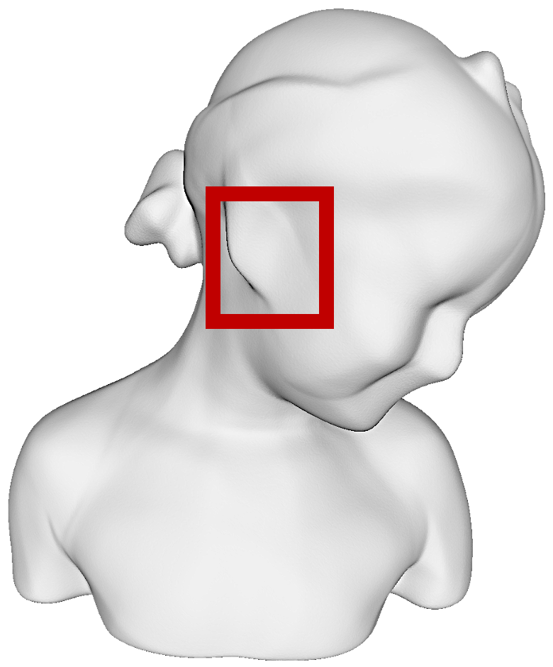
(a) No PE

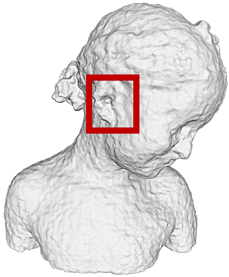
(b) PE with insufficient sampling

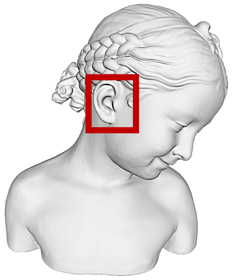
(c) PE with our sampling

Figure 1: The benefits brought by PE and our sampling strategy. This figure presents the extracted zero-level sets obtained from our trained signed distance function (SDF) on the Bimba model, using (a) vanilla MLP without PE, (b) PE-equipped MLP with insufficient training samples (33k points), and (c) PE-equipped MLP with our recommended sampling strategy, respectively. The sampling numbers for (a) and (b) are approximately 33k, uniformly distributed within the bounding boxes, whereas the training samples for (c) comprise approximately 900k uniformly distributed points and additional sample points on the surface. The network configuration for (a), (b), and (c) is an 8-layer MLP with 512 neurons in each layer. (a) MLP only captures a rough outline of the Bimba model; (b) a PE-equipped MLP captures more geometric details (see the ear) but also generates noisy artifacts; and (c) Incorporating our sampling strategy, the same PE-equipped MLP as in (b) not only recovers high-frequency features but also mitigate the noisy artifacts, yielding an accurate neural approximation of the Bimba model. Our goal is to provide an empirical and effective method for determining the sufficient rate of sampling.

However, an MLP alone often fails to capture high-frequency details of the target fields [10, 1, 4], which is coined as the spectral bias/frequency principle as explained by Rahaman et al. [11] or Xu et al. [12]. Take the task of fitting a Signed Distance Field (SDF) as an example. A single MLP network usually produces over-smoothed results, as shown in Fig. 1(a), especially in the regions of the SDF zero-level set which contains intricate geometry details. Similar observations have also been made in tasks like learning a neural radiance field [1]. To address this problem, the sinusoidal positional encoding, called PE for short, is introduced [1] for enhancing the ability of the MLP to capture these geometry details. Specifically, PE adds a layer of sinusoidal functions with various frequencies to an ordinary MLP. However, naïve application of PE in neural implicit representations often suffers from the side-effect of producing wavy artifacts  [13, 3, 10] as shown in Fig. 1(b).

In this paper, we present an in-depth analysis of the cause of the wavy artifacts. We observe that the wavy artifacts are caused by the aliased sampling of the response frequency [12] of a PE-equipped MLP network. Specifically, some high-frequency components in the response frequency, i.e., the output of such a network, are undersampled and aliased. Then, the training loss only minimizes the difference between the aliased network outputs and the target field, which leaves the underlying high-frequency components of the network outputs not suppressed, resulting in wavy artifacts and high test error at inference time.

\begin{overpic}[width=433.62pt,clip]{figures/freq_avg.png} \put(10.0,2.0){(a) Multiple Spectra} \put(57.0,2.0){(b) Intrinsic Spectrum} \end{overpic}

Figure 2: The response frequency and intrinsic frequency of a network. (a) Consistent response frequency spectra are observed among randomized PE-equipped MLPs with the same architecture (8 layers with 512 neurons per layer); (b) The averaged spectrum of the network over multiple sets of randomized network weights is used to estimate the intrinsic spectrum of the PE-equipped MLP.

Our first finding is that the randomly initialized PE-equipped MLP networks with the same architecture have very similar spectrum profiles to each other.

As shown in Fig. 2 (a), we randomly initialize the MLP networks 5 times with different random sets of weights and visualize their output frequency spectra. As we can see, these MLP networks all show similar spectrum profiles and bandwidths. Based on this observation, we compute the statistical expectation of these spectra in Fig. 2 (b) and term it the intrinsic spectrum to these PE-equipped MLP networks with this same architecture.

From Fig. 2 (b) we can see that the frequencies of the network are predominantly distributed in the low-value region but there are always some high-frequency components (up to 60 Hz) in the tail.

We validate the observation that when the training samples are insufficient to recover these high-frequency components in the intrinsic spectrum according to the Nyquist-Shannon (NS) sampling theorem [14], the learned SDFs often end up with wavy artifacts at test time. We show that the wavy artifacts can be removed by using sufficient sampling on these high-frequency components. This demonstrates that the aliasing effect is the cause of the wavy artifacts at test time. This motivates us to identify a cut-off frequency of the intrinsic spectrum to filter out those high-frequency components of negligible energy, thus not affecting the approximation quality. We also show that further increasing the training sampling rate beyond this cut-off frequency brings little additional improvement in the setting of SDF fitting. This suggests an effective strategy for sampling data points for training a neural implicit representation.

We devise an empirical method for probing the intrinsic spectrum of an MLP network and determining the cut-off frequency of this spectrum. We show experimentally that a PE-equipped MLP trained using the appropriate sampling rate recommended by our study can produce high-quality fitting of SDF that is superior to several widely used methods like SIREN [4], NGLOD [15], or MLP equipped with Spline-PE [16]. Furthermore, a comprehensive analysis is provided to validate the effectiveness of our designs in the recommendation of the highest intrinsic frequency (and thus the sampling rate) of PE-equipped MLP networks.

Our contributions are summarized as follows:

1) We present an insightful observation that the optimal sampling rate in SDF fitting is affected by both the target SDF frequency and the response frequency of MLP networks, the latter of which is characterized by the intrinsic spectrum of the PE-equipped MLP network.

2) We propose a practical method for estimating the intrinsic spectrum of a PE-equipped MLP and recommending the optimal sampling rate based on the cut-off frequency for the intrinsic spectrum, as suggested by the Nyquist-Shannon sampling theorem. This optimal sampling rate helps remove wavy artifacts to produce high-quality learned SDF fitting.

3) We provide extensive quantitative comparisons with state-of-the-art methods for SDF fitting and show the superiority of a PE-equipped MLP as an accurate 3D representation if trained properly with a sufficient data sampling rate.

II Related works

Recent studies [17, 18, 2, 19, 20, 21, 5, 22, 3, 13, 23, 24, 16, 4, 25] have demonstrated that it is promising to represent 3D shapes or scenes as implicit functions (e.g., signed distance functions or occupancy fields) parameterized by a deep neural network. These recent efforts show that a well-trained network can drastically compress the memory footprint to several megabytes for representing 3D shapes. To attain a high-fidelity neural representation, especially well reconstructing the geometric details in the given shape, many techniques have been developed, such as positional encoding (PE) techniques that map the input to a higher dimensional vector [1, 10, 16] or specially designed activation functions [4, 26].

In this work, we consider fitting an MLP network with sinusoidal PE [1] to represent a 3D shape. In particular, we explore how spatial samples and sinusoidal PE (or PE for short) can work together to enable MLP networks to capture fine-scale geometric features. We compare our method with several representative methods, e.g., [4, 16].

Another line of work [27, 28, 29, 7, 15, 30, 31] leverages the learned latent features for enhancing the expressiveness on fine-scale details. In particular, these studies usually learn a shallow MLP network and a set of latent feature vectors, each associated with a spatial coordinate, forming an explicit grid map. Given a spatial query, the corresponding latent feature vector is obtained, such as by interpolating nearby latent feature vectors stored in the grid map. Then, this latent feature vector is mapped by the MLP head to the value of the implicit function at this spatial query. While the results are compelling, this is achieved at the expense of explicitly storing a grid feature map. Artifacts at the interface of two adjacent grids may be observed as well.

Among them, NGLOD [15] is proposed to represent a single complex 3D shape as the signed distance function induced by the shape using a hierarchically organized feature map. It achieves the SOTA performance in both surface reconstruction and SDF approximation. We will validate our design choices by comparing our method with NGLOD.

Spectral bias of the MLP networks. [11] and [12] unveiled the characteristics of an MLP that learns low-frequency signals of the dataset first and gradually fits the high-frequency components. This characteristic is coined as Spectral bias [11] or Frequency principle [12]. [32] approach this problem from the Neural Tangent Kernel viewpoint. [10] then applied this explanation to the training dynamics of neural implicit representation, answering why low-frequency contents are learned in the first place. However, this line of work emphasizes the learning dynamics of the MLPs or neural implicit representations, while offering limited insight into why positional encoding schemes, in general, will lead to noisy outputs.

A recent work [33] demonstrated, via a Fourier lens, that the noisy outputs are due to the spectral energy shift from the low-frequency end to a high-frequency range when positional encoding layers are added. This observation, along with its analysis based on a two-layer network, conforms to ours in the frequency probing of various 1D examples and 3D SDF learning tasks. In contrast to [33] where a regularization term is proposed to incorporate a smooth geometric prior for training, we first discuss in depth that the cause of the noisy outputs is due to the aliasing effect during training. Then, we propose a simple yet effective sampling strategy to overcome the aliasing effect that ensures satisfactory results at inference time.

We also observed works on leveraging non-Fourier positional encoding schemes [34] or incorporating bandlimited filters [35] for image fitting tasks. Our work is complementary to these recent studies, revisiting the sinusoidal positional encoding scheme and unveiling the reason for its widely observed artifacts. Our outcome provides a practical choice for practitioners when using sinusoidal positional encoding to train their neural networks [36, 37].

III Methodology

III-A Learning SDF with Sinusoidal PE

\begin{overpic}[width=433.62pt]{figures/dft_new.png} \put(10.0,1.0){(a) D = 3} \put(43.0,1.0){(b) D = 4} \put(75.0,1.0){(c) D = 5} \par\end{overpic}

Figure 3: Intrinsic spectra of PE-equipped MLPs with different D. (a) to (c) illustrate the intrinsic spectra of the PE-equipped MLPs, each equipped with a PE with $D$ from 3 to 5. We plot the frequency corresponding to the PE in vertical black lines. The visualizations clearly demonstrate that frequencies beyond the PE frequency (the black lines) exhibit non-negligible magnitudes, suggesting that the intrinsic spectrum of PE-equipped MLPs extends far beyond the frequency associated with its corresponding PE. We also plot the cut-off frequency of each spectrum calculated by our method with vertical dashed lines. The magnitude beyond the cut-off frequency exhibits negligible values.

A signed distance field (SDF) returns the signed distance of a query point $\mathbf{x}\in\mathbb{R}^{3}$ to a given surface in 3D space. We follow the convention of defining the sign to be positive if the query point is outside the shape and negative otherwise; therefore the surface is the zero-level set of the SDF. One can encode a signed distance function as an MLP network denoted $f_{\theta}(\cdot)$, parameterized by the network weights. It has been shown that equipping an MLP network with sinusoidal positional encoding [1, 10] can improve the network’s representation ability for representing complex shapes. Such a PE-equipped MLP can be written as a composite function

$$y=f_{\theta}(\gamma_{D}(\mathbf{x})),$$ (1)

Here, the sinusoidal positional encoding is represented as

$$\gamma_{D}(\mathbf{x})=[\mathbf{x},PE_{0}(\mathbf{x}),PE_{1}(\mathbf{x}),\cdot\cdot\cdot,PE_{D}(\mathbf{x})],$$

where $PE_{p}(x)=[\sin(2^{p}\pi x),\cos(2^{p}\pi x)]$ and $x$ is one of the components of $\mathbf{x}$. The highest frequency of the combined signal of the PE encoding is $2^{(D-1)}$.

The following SDF loss is adopted in fitting an SDF field with the neural network,

$$E=\int_{\Omega}|SDF(\mathbf{x})-f_{\theta}(\gamma_{D}(\mathbf{x}))|d\mathbf{x},$$ (2)

where $\Omega$ is the spatial domain and $SDF(\mathbf{x})$ is the ground-truth (GT) SDF at $\mathbf{x}$. While incorporating a PE layer with high-frequency components benefits the fitting of high-frequency details, it also brings a side effect of noises [10] or wavy artifacts [13] as shown in Fig. 1(b).

Overview. It has been empirically observed that increasing the sampling rate can mitigate the noisy artifacts of the SDF encoded by a PE-equipped MLP. In this work we take a step further by first investigating the relevant mechanism of the network to understand the cause of this side effect of adding PE, and them estimating quantitatively the sufficient sampling rate for suppressing these artifacts. We show that this side effect of adding PE can be viewed as an aliasing problem. In particular, we observe that this aliasing problem is caused during the minimization of Eq. 2 where the loss is optimized concerning a set of aliased frequency components in $f_{\theta}(\gamma_{D}(\mathbf{x}))$, the output of the network, due to an insufficient sampling rate.

In the following, we will provide an intuitive analysis of $f_{\theta}(\gamma_{D}(\mathbf{x}))$ and the potential aliasing effect at training that explains the wavy artifacts. Then, we propose a practical solution to efficiently assessing the intrinsic spectrum of a PE-equipped MLP and an effective method for determining the cut-off frequency of the intrinsic spectrum of the MLP to obtain the optimal sampling rate for training the MLP. Finally, we devise a simple sampling and training strategy to achieve high-quality SDF fitting using a PE-equipped MLP.

III-B Training Aliasing Effect

An aliasing problem is caused by the failure of sampling signal components with frequencies higher than the sampling rate. According to the Nyquist-Shannon (NS) sampling theorem [14], at least a uniform sampling rate of $2F$ is required to reconstruct the given signal with frequency $F$.

Let $f_{\theta}(\cdot)$ denote an MLP without the PE layer, parameterized by the weights and biases $\theta=\{\mathbf{W}_{i},\mathbf{b}_{i}\}_{i=1}^{L}$. Let $\gamma(\mathbf{x})$ denote the PE layer, which has no free parameters to optimize. Then we denote the PE-equipped MLP by

$$h_{PE}(x)\equiv f_{\theta}(\gamma(\mathbf{x})).$$

The optimization problem of fitting an implicit field $\bar{y}(\mathbf{x})$ is achieved by minimizing the following loss function

$$E(\mathbf{x})=\arg\min_{\theta}|h_{PE}(\mathbf{x})-\bar{y}(\mathbf{x})|.$$ (3)

Optimizing the network parameters $\theta$ requires a sufficiently dense sampling of the function $h_{PE}(\mathbf{x})$, which is based on the highest frequency of $h_{PE}(\mathbf{x})$, as suggested by the Nyquist-Shannon sampling theorem. Note that $h_{PE}(\mathbf{x})\equiv f_{\theta}(\gamma(\mathbf{x}))$ usually carries components of much higher frequency than those of the PE signal $\gamma(\mathbf{x})$ due to the action of multiple layers of the MLP $f_{\theta}(\cdot)$ applied to $\gamma(\mathbf{x})$.

When an insufficient sampling rate with respect to $h_{PE}(\mathbf{x})$ is applied for training $h_{PE}(\mathbf{x})$, it will result in an aliased function of lower frequency, denoted $h_{PE}^{lf}(\mathbf{x})$. Conceptually, we have the decomposition

$$h_{PE}(\mathbf{x})=h_{PE}^{lf}(\mathbf{x})+h_{PE}^{hf}(\mathbf{x})$$

where $h_{PE}^{hf}(\mathbf{x})$ contains the components of $h_{PE}(\mathbf{x})$ that are of higher frequency than those contained in the aliased function $h_{PE}^{lf}(\mathbf{x})$.

Hence, the optimization problem under this under-sampling condition turns out to be minimizing an aliased target function $h_{PE}^{lf}(\mathbf{x})$ as follows

$$\tilde{E}(x)=\arg\min_{\theta}|h_{PE}^{lf}(\mathbf{x})-\bar{y}(\mathbf{x})|.$$ (4)

This leaves the higher-frequency components of $h_{PE}^{hf}(\mathbf{x})$ untrained. Consequently, given a query $\mathbf{x}$ unseen at the training stage, the fitting error $E(\mathbf{x})$ generated by the high-frequency components $h_{PE}^{hf}(\mathbf{x})$ will be present in the final output of the PE-equipped network $h_{PE}(\mathbf{x})$ at inference time, leading to wavy artifacts of the SDF approximation.

From this analysis, it is clear that an insufficient number of training samples will lead to wavy artifacts at inference time due to the aliasing effect during training. Hence, to determine the sufficient sampling rate, we need a method for examining the frequency characteristics of $f_{\theta}(\gamma_{D}(\mathbf{x}))$ and determining the appropriate sampling frequency.

III-C Intrinsic Spectrum and Cut-off Frequency

Intrinsic spectrum. Due to the complicated interactions between the layer inputs and the interleaved linear/non-linear operations, it is difficult, if not intractable, to theoretically analyze the frequency characteristics intrinsic to a network architecture $f_{\theta}(\gamma(x))$. Therefore, we devise an empirical approach to probing the frequency characteristics by studying specific randomized networks. It is observed that the frequency spectra of these networks with randomized weights have similar spectra.

Given a randomized network $f_{\theta}$, we first use densely distributed regular points $\mathbf{x}_{j}$ to produce a discrete set of network output $y_{j}$, from which we obtain a sequence of discrete frequencies of the spectrum of $f_{\theta}$ by the Fourier transform. Next, we compute the power at each discrete frequency $F$ as follows,

$$S(F|\theta)=|p(F|\theta)|^{2},$$ (5)

where $p(F|\theta)$ is the frequency magnitude at $F$. Then, for each frequency $F$, we compute the expectation of the power spectrum as follows

$$\mathbb{E}(F)=\frac{1}{C}\int S(F|\theta)p(\theta)d\theta,$$ (6)

where $C$ is the normalizing factor and $p(\theta)$ is the probability density function for the parameter sampled from a predefined distribution $\theta\sim\Theta$. In our implementation, each output signal of such a network is produced with a set of dense points sampled on a line through the bounding domain of the network input.

As we can see from Fig. 2 (a), when a network is assigned different sets of random weights, which are drawn from the same distribution, their frequency spectra are similar to each other, showing a limited bandwidth within a relatively tight range towards the low-frequency end. Furthermore, as shown in Fig. 2 (b), the fact that the expectation of the frequency spectra possesses this bandlimited property is intrinsic to the PE-equipped networks initialized from the same distribution. Therefore, this intrinsic property observed from the frequency spectrum allows us to estimate a cut-off frequency for determining the appropriate training sampling rate to mitigate the aliasing effect at inference time. In Fig. 3, we show the intrinsic spectra of PE-equipped MLP with different frequency levels $D$ of PE.

Cut-off frequency and sampling rate. Next, we define a cut-off frequency for this frequency spectrum to characterize the undersampling and oversampling conditions. The sampling rate corresponding to the cut-off frequency ensures the suppression of the wavy artifacts in the learned SDF by avoiding the undersampling or training aliasing issue. Meanwhile, we show that using a large sampling rate beyond this cut-off frequency will not noticeably further minimize the SDF fitting error for the given MLP network. Thus, knowing the cut-off frequency helps prevent oversampling to avoid wasting computing resources.

We derive the cut-off frequency as follows.

We aim to find a critical value at which the spectrum is almost constant (close to 0), but since the spectrum contains noise, we consider using a smooth function to fit the spectrum. We use the following function to fit the spectrum

$$y(x)=\frac{a}{{x^{2}+b}},$$ (7)

where $a$ and $b$ are the coefficients for fitting.

The fitted smooth curves are shown by the black curves in Fig. 5 (a) to (c). In order to find the critical value, we use the slope $k$ of the fitting curve to select the cut-off frequency. Specifically, we empirically set the corresponding frequency as the cut-off frequency when $k<6\times 10^{-4}$. This parameter has been found to work well in all of our experiments.

Our recommended sampling rate is defined as twice the cut-off frequency, according to the NS sampling theorem. We adopt the multi-dimensional generalization of the Nyquist-Shannon sampling theorem [38] as follows:

$$\mu=(2F_{c})^{\ell},$$ (8)

where $F_{c}$ is the cut-off frequency and $\ell$ indicates the input dimension of the task. Thus, $\ell=3$ in our setting of SDF approximation.

IV Experiments and results

In this section, we describe the evaluation datasets and metrics in Sec. IV-A. Experiments are conducted in the following aspects to demonstrate the effectiveness of our method. We begin with the validation of the proposed sampling rate in Sec. IV-B. Then, we compare our results with those produced by existing methods on the SDF fitting task in Sec. IV. Finally, comprehensive analyses of our method, including surface fitting quality and its applicability to various different network initializations and architectures, are provided in Sec. IV-D.

\begin{overpic}[width=433.62pt,clip]{figures/fandisk_box.png} \put(15.0,0.0){(a) GT shape} \put(65.0,0.0){(b) Active grid cells} \end{overpic}

Figure 4: Active grid cells for the shape Fandisk. We selected grid cells that intersect with the surface of the shape to enclose each shape with active grid cells.

\begin{overpic}[width=433.62pt,clip]{figures/sample_err_uniform.png} \put(10.0,50.0){(a) Spectrum (D=3)} \put(61.0,50.0){(c) Spectrum (D=4)} \put(10.0,4.0){(d) Spectrum (D=5)} \put(63.0,4.0){(d) SDF error} \par\end{overpic}

Figure 5: Validation of our recommended sampling rate. We show spectra of our default PE-equipped MLPs (8-layer MLP with 512 neurons per layer) using different $D$ (the channel width of PE) in (a) to (c) and the plots of SDF errors in (d). The horizontal axis of each spectrum plot from (a) to (c) is the frequency, while the vertical axis represents the corresponding magnitude of each frequency $F$. We also plot the fitting curves of the spectra using black curves from (a) to (c). In (d), the horizontal axis represents the sampling rate ($2F$) and the vertical axis denotes the SDF fitting error. We plot the cut-off frequency $F_{\rm c}$ determined in  III-C as the dashed vertical line in all plots. This validates that our recommended sampling rate ensures the convergence of the SDF errors.

\begin{overpic}[width=433.62pt,clip]{figures/sdf_progress.png} \put(10.0,1.0){(a) GT} \put(24.0,1.0){(b) PE sampling} \put(55.0,1.0){(c) Our sampling} \put(78.0,1.0){(d) Denser sampling} \par\put(41.0,4.0){29.3E-4} \put(67.0,4.0){5.6E-4} \put(92.0,4.0){5.5E-4} \par\par\par\end{overpic}

Figure 6: SDF fitting results of different sampling rates. (a) The ground-truth SDF on the profile plane (left) and the corresponding surface shape (right). In (b,c,d), we show the corresponding fitted SDF values (left), the reconstructed surfaces (top-right), and the error maps (bottom-right). We also put the SDF error below each error map. We use PE frequency with $D$=5, and the corresponding cut-off frequency is 63$Hz$. “PE sampling” uses the sampling rate recommended by the highest PE frequency $D$, approximately 20k samples. “Our sampling” uses the sampling rate computed from the proposed intrinsic cut-off frequency, approximately 900k. “Denser sampling” refers to a higher sampling rate over “Our sampling”, which is around 1800K samples. Compared to (b), “Our sampling” (c) can effectively mitigate the noisy artifacts both on the reconstructed surface as well as the learned SDF. Comparison between (c) and (d) shows that further increasing the sampling rate (c) brings little improvement to both the surface reconstruction and the learned SDF.

IV-A Implementation details

Normalizing network outputs. Before computing the frequency spectrum of the signals $\{\mathbf{x}_{j},y_{j}\}$, we first whiten the output $y_{j}$ by subtracting the mean and scaling them so that their standard deviation equals 1. Note that these operations are linear and used to normalize the total energy the sequential signals $\{\mathbf{x}_{j},y_{j}\}$ carry; they will not modify the frequency characteristic of the signal concerned. This way, the sequential data obtained from different randomized networks are now normalized and comparable to each other.

Training details. Given the surface of a 3D shape, we first normalize it to a cubical domain with its maximal extent being $[-1,1]$. The entire cubical domain is partitioned into a regular grid of $20\times 20\times 20$ cells. Training samples are exclusively located in those grid cells that intersect with the surface, as depicted in Fig. 4. These intersecting grid cells are referred to as active grid cells. Given a PE-MLP network, we calculate the recommended sampling rate as described and apply it to deriving a set of training samples uniformly sampled within each grid cell.

By default, we use an 8-layer MLP network equipped with $\gamma_{D=5}$. Each layer of the MLP has 512 neurons and is followed by the softplus activation ($\beta=100$ as suggested in [22]) with an exception at the last layer where a tanh activation is applied. During training, we employ a mini-batch of $100,000$ sample points. Each network is trained for $30,000$ iterations, which takes approximately 30 mins in total time. The ADAM optimizer [39] is used for training. The training starts with a learning rate of $0.0001$ and then decays by a factor of 0.1 after $27,000$ iterations. All networks are implemented with PyTorch [40] and trained on an NVIDIA RTX3090 graphic card (24 GB memory).

Evaluation protocols. To evaluate the quality of the SDF fitting results, we adopt the mean absolute SDF error, $\epsilon_{SDF}$, between the predicted signed distance values and the corresponding ground-truth (GT) values at validation points. The validation set consists of $100,000$ points which are sampled in the active grid cells without overlaps with the training samples.

For evaluating the surface reconstruction quality, we use the Marching Cube [41] to extract the reconstructed surface at the zero-level set from the learned signed distance field. Our dataset comprises eight commonly employed shapes in computer graphics.

IV-B Validation of our sampling rate

To validate the effectiveness of the proposed sampling rate as described in Section III-C,

we present the results on the Lucy shape for illustrative purposes in Fig. 5, and results on another two shapes are presented in the Appendix, where we observe the same trend between the sampling rate and the SDF error on these shapes. The setting of PE-MLP networks follows the default setting except that different highest frequencies $D$ are used for the PE layer.

Fig. 5 (a) to (c) illustrate the frequency spectrum of the output signal (or the response frequency) of the same PE-equipped MLP with a different set of randomized weights and biases. Each dashed vertical line represents the sampling rate ($2F$) corresponding to cut-off frequency $F$ for a PE-equipped MLP with a different $D$ value in its PE layer.

Remarkably, each dashed vertical line in Fig. 5 (d) corresponding to the cut-off frequency precisely captures the point of test error convergence for each PE-equipped MLP, indicating that further increasing the sampling rate will not significantly further enhance SDF accuracy, thus validating our design choice.

We further provide qualitative results of SDF fitting in Fig. 6 Here, the same network architecture is used which has a PE layer of $D=5$ and eight hidden layers, each with 512 neurons. The three learned SDFs shown in this figure are trained with different amounts of training samples: one using the sampling rate corresponding to the highest PE frequency $D$ (b), one with the sampling rate dictated by the network cut-off frequency (c), and another with a higher sampling rate (d). Notably, the SDF from the sampling rate based on the highest PE frequency exhibits undulating artifacts with an RMSE of 29.3E-4, whereas the errors of the suggested or even denser sampling rates have RMSEs of 5.6E-4 and 5.5E-4 respectively, which are similar to each other but significantly lower than the results with PE sampling rate.

The results demonstrate that our recommended sampling rate serves as a sufficient and cost-effective lower bound of sample point numbers for high-fidelity SDF reconstruction.

IV-C Comparison with existing methods

We compare our methods with three baseline approaches, i.e., SPE [16], SIREN [4], and NGLOD [15]. SPE [16] proposes an alternative positional encoding scheme based on the B-spline basis function. SIREN [4] proposes to use a sine activation function to replace the softplus activation function used in ours and SPE’s networks and avoid employing any positional encoding schemes. NGLOD [15] is a representative method of another line of work that makes use of explicit, learnable feature grids organized in an octree, along with a compact shared MLP network to fit the SDF.

Implementation of baseline methods. SPE and SIREN are trained with the same sample points and loss functions as our method.

We adopt their default learning rate, $1\times 10^{-4}$ for SPE and $0.5\times 10^{-4}$ for SIREN, for training.

Our method, SPE, and SIREN all are trained for $30,000$ iterations and observed to have fully converged. Since NGLOD learns a hierarchical feature grid different from ours and the other two methods, we follow their default training strategy provided in their official implementation with five levels of detail and train NGLOD to convergence (for 250 epochs). Under this default setting, NGLOD uses 2.5 million sample points for training.

The results in Table I show that our method outperforms the three baseline approaches in the SDF fitting task. Some qualitative results are shown in Fig. 7. The qualitative results further confirm that the amount of training samples suggested by our method enables accurate SDF fitting with a simple PE-equipped MLP network.

	Ours	SIREN [4]	SPE [16]	NGLOD [15]
Fandisk	4.10E-4	6.58E-4	7.27E-4	7.49E-4
Lucy	8.68E-4	8.69E-4	9.90E-4	11.2E-4
Happy Buddha	6.72E-4	9.62E-4	9.59E-4	11.3E-4
Hand	3.78E-4	6.50E-4	4.80E-4	7.96E-4
Bimba	5.63E-4	5.95E-4	7.62E-4	8.54E-4
ABC1	3.18E-4	4.39E-4	7.65E-4	5.91E-4
ABC2	2.65E-4	4.73E-4	6.01E-4	7.03E-4
Armadillo	6.83E-4	7.25E-4	9.89E-4	11.19E-4
Woman	3.71E-4	5.93E-4	6.10E-4	11.01E-4

TABLE I: Comparison on the SDF fitting task. Mean absolute SDF error between the fitted SDF fields and the corresponding ground-truth SDF fields on evenly sampled validation points. Our PE-MLP networks with the suggested sufficient sampling rate outperform other comparing baselines by a large margin.

\begin{overpic}[width=433.62pt,clip]{figures/sdf_contour.png} \put(10.0,3.0){(a) GT} \put(27.0,3.0){(b) NGLOD} \put(48.0,3.0){(c) SPE} \put(63.0,3.0){(d) SIREN} \put(83.0,3.0){(e) Ours} \par\end{overpic}

Figure 7: Qualitative comparison between our results and those of the baseline methods on SDF fitting task. The first column shows the GT shapes and the cross-sectioning planes colored in black. The SDF error maps of the points on the cross-sectioning plane are visualized. The error values are clipped by a maximum of 0.003. A warmer color indicates a higher error.

\begin{overpic}[width=433.62pt,clip]{figures/surface_geo.png} \put(8.0,3.0){(a) GT} \put(25.0,3.0){(b) NGLOD} \put(45.0,3.0){(c) SPE} \put(65.0,3.0){(d) SIREN} \put(85.0,3.0){(e) Ours} \end{overpic}

Figure 8: Qualitative comparison between our results and those of the baseline methods on the surface fitting task. The first line showcases the extracted geometry of the $Woman$ model. Zooming in, the second line provides a closer view of the aforementioned geometry. The third line displays error maps of the extracted meshes, where the red color indicates a higher error and the blue color indicates a lower error. Analyzing the geometry of the $Woman$ model, it becomes evident that both NGLOD and SPE lack the ability to accurately represent high-frequency details. On the other hand, while SIREN and our method are capable of depicting geometric details precisely, SIREN exhibits wavy artifacts across flat areas, as can be observed from the error maps in the third line. Contrarily, our method excels not only in recovering high-frequency details but also in maintaining stability on flat planes, showing our superiority over our baselines in the task of surface fitting.

\begin{overpic}[width=433.62pt,clip]{figures/surface_error_map.png} \put(6.0,2.0){(a) NGLOD} \put(33.0,2.0){(b) SPE} \put(52.0,2.0){(c) SIREN} \put(76.0,2.0){(d) Ours} \end{overpic}

Figure 9: Qualitative comparison between our results and those by the baseline methods on the surface fitting task. We draw the error maps of the Chamfer Distances between the extracted surfaces and the GT meshes. We clip the error by the maximum of 0.003. The red color indicates the high error while the blue color indicates the low error.

\begin{overpic}[width=433.62pt,clip]{figures/sample_error_smaller.png} \put(13.0,1.0){(a) Spectrum } \put(63.0,1.0){(b) SDF Error} \end{overpic}

Figure 10: Smaller network. We present the spectrum and corresponding SDF error curve for a reduced-size PE-equipped MLP (consisting of a 4-layer MLP with 128 neurons per layer) with $D=4$ in (a) and (b). Consistent with the observations made on our default network, we find that our recommended sampling rate enables the PE-equipped MLP to attain near-saturation SDF error even on the smaller network.

\begin{overpic}[width=433.62pt,clip]{figures/siren_fpe.png} \put(0.0,69.0){(a) Spectrum of FPE ($\sigma$=10)} \put(40.0,69.0){(b) Error Curve of FPE ($\sigma$=10)} \put(0.0,36.0){(c) Spectrum of FPE ($\sigma$=19)} \put(40.0,36.0){(d) Error Curve of FPE ($\sigma$=19)} \put(3.0,4.0){(e) Spectrum of SIREN} \put(42.0,4.0){(f) Error Curve of SIREN} \end{overpic}

Figure 11: Other network configurations. We further apply our sampling rule to the FPE-MLP [10] network and the SIREN [4] network. The first row represents the analysis of the FPE-MLP network, while the second row corresponds to the analysis of the SIREN network. We plot the computed cut-off frequencies in the spectrums of different networks ((a), (c), and (e)), along with the corresponding sampling rates in the error curves ((b), (d), and (f)). The determined cut-off frequencies accurately capture the convergence points in each SDF error curve, indicating that our rule has the potential to generalize to other network architectures.

\begin{overpic}[width=433.62pt,clip]{figures/xavier_init_new.png} \par\put(15.0,1.0){(a) Spectrum} \put(63.0,1.0){(b) SDF Error} \par\end{overpic}

Figure 12: Xavier uniform initialization. We present the spectrum of a PE-equipped MLP ($D$ = 4) with Xavier initialization in (a) and the corresponding SDF error curve in (b). The vertical line in (a) indicates the cut-off frequencies of the spectrum. The vertical line (b) corresponds to the sampling rate associated with the cut-off frequencies, which effectively pinpoints the convergence points of the error curve.

IV-D Discussions

In the following discussion, we provide additional analysis of the surface fitting quality, validation of our sampling distribution, the relationship between shape frequency and network complexity, and the relationship between the network intrinsic frequency and the size of trainable parameters.

Can our method produce high-quality surfaces? To show that our method also enables accurate surface fitting, we further conduct a surface fitting experiment and compare our performance with the same baseline methods. In this experiment, we incorporate 10 million surface samples on the target shape in training our method and the baseline methods, which is the same as [4]. We report the quality of surface fitting results using the Chamfer Distance (CD) in Table II. The results show that our method also outperforms all baseline methods on the surface fitting task. To provide additional visual evidence, we present a set of surfaces extracted from the learned SDF in Fig. 8. These visualizations highlight the ability of our method to capture high-frequency details while reproducing smooth, low-frequency areas. In comparison, while being able to represent geometric details to some extent, the baseline methods fail to accurately depict intricate features, as demonstrated in the zoomed-in views of Fig. 8 (the second row). Furthermore, as depicted in the third row of Fig. 8, SIREN exhibits noticeable errors in the flat area. More comparison results are shown in Fig. 9.

	Ours	SIREN [4]	SPE [16]	NGLOD [15]
Fandisk	2.29E-5	55.3E-5	25.5E-5	25.7E-5
Lucy	7.90E-5	92.5E-5	103.2E-5	45.5E-5
Happy Buddha	9.18E-5	56.1E-5	91.1E-5	41.9E-5
Hand	9.48E-5	67.3E-5	40.1E-5	21.1E-5
Bimba	6.24E-5	46.4E-5	53.6E-5	31.5E-5
ABC1	4.49E-5	62.6E-5	34.9E-5	24.2E-5
ABC2	2.39E-5	76.1E-5	9.78E-5	25.6E-5
Armadillo	17.4E-5	49.7E-5	84.3E-5	37.7E-5
Woman	5.20E-5	35.0E-5	34.7E-5	25.3E-5

TABLE II: Comparison on the surface fitting task. The Chamfer Distances (CD) between the fitted surfaces and ground-truth surfaces are reported.

Why not choose on-the-fly sampling? Given that we have established the requirement for the sampling rate to meet the lower bound set by the network’s initial intrinsic frequency, it is natural to question why we do not opt for an on-the-fly sampling strategy similar to that initially employed in NGLOD[15]. The primary reason is that, in the task of SDF fitting, performing on-the-fly sampling at every iteration would be time-consuming, even with a GPU-accelerated algorithm. For instance, if we were to resample the training points at each iteration, the time spent on sampling would be 2.5 times longer than the training time in the case of NGLOD [15]. While it is possible to decrease the sampling time by adopting interval-based sampling, as exemplified in the current implementation of NGLOD [15], the question arises: What is the appropriate duration for each interval? To address this inquiry, we must revisit the challenge of determining the optimal quantity of sampling points for effective training. Resolving this matter constitutes the primary emphasis of the present paper.

Is our recommended sampling rate applicable to other settings?

1) Smaller networks. As shown in Fig. 10, to demonstrate that the sampling rate suggested by our approach is also applicable to smaller networks other than the default 8-layer MLP, we apply the same approach to analyzing the frequency of a smaller MLP network and conduct the same SDF fitting experiment using different sampling rates. This smaller network has 4 hidden layers with 128 neurons per layer. We observed the same trend as observed in the experiments in Sec. IV-B that SDF fitting errors converge as the sampling rate increases beyond the suggested rate based on the cut-off frequency determined by our approach.

2) Other network architectures. To examine to what extent the proposed sampling scheme is effective, we further apply the sampling scheme to some other MLP network architectures. Specifically, Fig. 11 shows two MLP networks using Random Fourier Features as their positional encoding [10] (the top two rows) and a SIREN network [4] (the bottom row). As we can see, the SDF fitting errors decrease and converge as the sampling rate reaches the proposed sampling rate, which demonstrates that the proposed intrinsic spectrum and cut-off frequency are also applicable to these two architectures.

3) Different initialization methods. So far, we have seen that our approach applies to different network settings. One may be curious about whether our proposed approach is still applicable when the initialization scheme of the weights and biases of a network changes. Hence, as an example, we use Xavier uniform initialization [42] to replace the default uniform initialization used in previous experiments. Fig. 12 empirically verifies the effectiveness of our approach in determining a cut-off frequency for preparing training samples.

\begin{overpic}[width=433.62pt,clip]{figures/diff_net.png} \put(14.0,9.0){14.9E-4} \put(44.0,9.0){6.83E-4} \put(74.0,9.0){6.90E-4} \put(14.0,2.0){(a) Small} \put(40.0,2.0){(b) Appropriate} \put(72.0,2.0){(c) Large} \end{overpic}

Figure 13: The MLP network should be capable enough for an accurate fitting. We show the visualizations of the SDF error of our SDF fitting task in the first line and the corresponding SDF error values in the second line. For better visualization, we only show the SDF error of surface points. The color red indicates a large error while the color blue indicates a small error. From the figure, we can see that the network complexity choice (b) results in a relatively small error for the SDF fitting task. Increasing the network complexity further (c) does not lead to a significant decrease in error, as the network’s complexity already covers the shape’s frequency. However, when the network complexity does not yet cover the shape frequency as in (a), the SDF fitting task exhibits a large error.

From shape frequency to network complexity. Though our method provides a lower bound for the sampling rate, the sample point number is not the only factor that affects the final SDF fitting quality. We note that to ensure high fitting accuracy, the network needs to be designed to be deep and wide enough to possess adequate capacity to fit the SDF of a given shape. In Fig. 13, we show the results of using networks of different capacities, all of which use the recommended sampling rate. The network referred to as “Small” in Fig. 13 (a) is a PE-equipped MLP with 4 layers, each containing 128 neurons. The network referred to as “Appropriate” in Fig. 13 (b) is an MLP consisting of 8 layers, with each layer containing 512 neurons. To further enhance the network’s capacity, we upgrade it to an MLP with 10 layers, maintaining 512 neurons per layer, referred to as “Large” in Fig. 13 (c). As the fitting results show, the small network’s complexity proved to be inadequate for capturing the frequency of the target shape, resulting in a significant fitting error. The network in (b) already fulfills the requirements for shape frequency and thus exhibits a low error. Further increasing the number of layers in the network does not produce a noticeable improvement in accuracy, as shown in Fig. 13 (c).

V Conclusions

We investigated the role of spatial samples with ground-truth signed distance values in learning a quality signed distance field induced by the given shape and how the spatial samples can work in synergy with the sinusoidal positional encoding for this purpose. While it has been well known in a qualitative sense that more training samples can lead to better results of SDF approximation, we propose an efficient method for quantitatively estimating a sufficient sampling rate for training the neural network by analyzing its intrinsic spectrum and determining the cut-off frequency on the spectrum. We approach the problem by employing the Nyquist-Shannon to the intrinsic frequency of the PE-equipped MLP, which is attained by applying FFT analysis to the output of the PE-MLP with random initialization. We also demonstrate that by training with our recommended sample rate, the coordinate networks can achieve state-of-the-art performance regarding SDF accuracy. This provides a strong baseline for future studies in this field.

Future work. The presented study has explored only the interplay between the spatial sample rate and the sinusoidal positional encoding but we do not provide a concrete rule to explain the sample point number on the surface in the surface fitting task. In future works, we can also study how surface sample number affects the surface quality from a frequency perspective.

VI Appendix

\begin{overpic}[width=433.62pt,clip]{figures/our_gallery.png} \end{overpic}

Figure 14: The fitted surfaces of our method in the surface fitting task. These shapes contain various geometric details, such as flat regions, sharp features, high-frequency details, etc.

VI-A More Implementation Details

Dataset. The dataset utilized in our experiments comprises 9 shapes that encompass a range of geometric details, as illustrated in Fig. 14. Specifically, we obtained the models for Happy Buddha[43], Armadillo, and Lucy from the Stanford 3D Scanning Repository. The Fandisk model was published in[44]. Both the Bimba and Fandisk models were retrieved from the following GitHub repository: https://github.com/alecjacobson/common-3d-test-models/. Additionally, we conducted tests using the Woman Relief model, which was purchased online. Furthermore, we included two CAD models, namely ABC1 and ABC2, from the ABC dataset [45]. Lastly, the Hand shape was generated by [46].

VI-B More Experiments and Results

In the following section, we present a series of supplementary experiments to validate our sampling rate, sampling distributions, and the extension from one dimension to three dimensions.

Validation of our sampling rate on more shapes. We validate our sampling rate on additional shapes, namely Bimba and Armadillo. The SDF error curves for these shapes are illustrated in Fig. 15. It can be seen from the figure that our recommended sampling rates consistently correspond to the convergence points of the error curves, further confirming the superiority of our sampling method.

\begin{overpic}[width=433.62pt,clip]{figures/more_shapes.png} \put(20.0,2.0){(a) Bimba} \put(65.0,2.0){(b) Armadillo} \end{overpic}

Figure 15: Validation of our sampling rate on more shapes. We show the SDF error curves of Bimba and Armadillo in (a) and (b). The vertical lines are our recommended sampling rates. They align well with the convergence points on the error curves.

\begin{overpic}[width=433.62pt,clip]{figures/offset_compare.png} \put(10.0,4.0){(a) GT} \put(40.0,4.0){(b) Offset} \put(75.0,4.0){(c) Ours} \end{overpic}

Figure 16: Qualitative comparison of learned SDFs with different sampling schemes on Fandisk. In (b) and (c), the left column is the contour of the SDF slice as cut by the black plane in (a), and the right column is the corresponding error map of the SDF slice. The red indicates a higher error while the blue indicates a lower error. Our result (c) approximates the GT SDF (a) well compared with the Offset scheme (b).

Extension to PE-equipped MLP with 3D input. We determine the cut-off frequency corresponding to the sampling rate by analyzing the frequency spectrum of the PE-MLP with a 1D input. However, when performing SDF fitting for a specific shape, our input becomes 3D. To show that the 3D frequency analysis is consistent to the 1D version, we sampled points along the x, y, z, and diagonal axes in the 3D domain and performed a 1D FFT analysis on the obtained signals. As depicted in Fig.17 (a) and (b), the cut-off frequency of a specific axis of the 3D input remains consistent with that of the 1D input, as shown in Fig. 17 (c) and (d). We also calculated the frequencies along the diagonal axis in the 3D domain. As illustrated in Fig. 17 (e) and (f), the frequencies along the diagonal axis are lower than those along the x, y, and z axes because we use the axis-aligned positional encoding. Hence, when determining the sampling density in the 3D domain, it is sufficient to use the frequencies along the x, y, and z axes to ensure it captures the highest frequency in space.

	Fandisk	Lucy	Happy Buddha	Hand	Bimba
Ours	4.10E-4	8.68E-4	6.72E-4	3.78E-4	5.63E-4
Offset	4.67E-4	9.26E-4	7.90E-4	5.62E-4	5.81E-4

TABLE III: To effectively control the high frequencies introduced by PE-MLP, uniform sampling is used. We conducted a comparison of the SDF error between two sampling distributions. The first distribution is our uniform sampling, while the second, called “Offset”, is the Gaussian distribution [2]. Both sampling distributions use an equal number of sampling points recommended by our sampling strategy. By utilizing uniform sampling, we can ensure stable control over the artifacts caused by PE-MLP, thereby recommending an optimal sampling number.

\begin{overpic}[width=433.62pt,clip]{figures/1d_3d_fft.png} \put(10.0,2.0){(a) 1D Input } \put(40.0,2.0){(b) 3D Input on Axes} \put(73.0,2.0){(c) 3D Input on Diagonal} \par\end{overpic}

Figure 17: Extending our 1D FFT analysis to a PE-equipped MLP with 3D input. We plot the spectrum of the output of the PE-equipped MLP with 3D input, where the points are sampled along the x-axis in (b), and the spectrum of the output of the PE-equipped MLP with 1D input in (a). Additionally, we display the spectrum of the output of the PE-equipped MLP with 3D input, where the points are sampled along the diagonal in (c). In order to better compare the cut-off frequencies of different spectra, we have marked the frequency 42 with a vertical line of light blue color. The results indicate that the behavior of the spectrum of the PE-equipped MLP with 3D input along the axes is the same as that of the PE-equipped MLP with 1D input. The spectrum of the sample points along the diagonal exhibits significantly lower cut-off frequencies. The reason is that we adopt the axis-aligned positional encoding. Thus, we choose the frequency on axes as the reference for computing our sampling rate to ensure that it is able to cover the high frequency on the XYZ axes.

Is our uniform sampling a good sample distribution? In our implementation, we use uniform sampling in generating training examples as suggested by NS theorem. However,

there is an alternative method [2] where surface samples are perturbed using offset vectors generated from a Gaussian distribution. We refer to this sampling scheme and its corresponding results as Offset in our experiments. From Tabble III, we see that our sampling scheme consistently produces better results regarding the RMSE of SDF values than the Offset scheme. Moreover, it is evident from Fig. 16 that utilizing the Offset sampling schema introduces wavy artifacts in regions where the SDF is distant from the surface. In contrast, our uniform distribution guarantees stability across the entire domain. This is because the high frequencies generated by PE-MLP are distributed throughout the domain. Consequently, even when a sufficient number of samples are present, we recommend utilizing a uniform distribution as a foundation to effectively cover the highest frequencies introduced by PE-MLP. Based on this, one can also apply additional emphasis on specific areas of interest.

References

- [1] B. Mildenhall, P. P. Srinivasan, M. Tancik, J. T. Barron, R. Ramamoorthi, and R. Ng, “Nerf: Representing scenes as neural radiance fields for view synthesis,” in European conference on computer vision. Springer, 2020, pp. 405–421.
- [2] J. J. Park, P. Florence, J. Straub, R. Newcombe, and S. Lovegrove, “Deepsdf: Learning continuous signed distance functions for shape representation,” in Proceedings of the IEEE/CVF Conference on Computer Vision and Pattern Recognition, 2019, pp. 165–174.
- [3] A. Gropp, L. Yariv, N. Haim, M. Atzmon, and Y. Lipman, “Implicit geometric regularization for learning shapes,” arXiv preprint arXiv:2002.10099, 2020.
- [4] V. Sitzmann, J. Martel, A. Bergman, D. Lindell, and G. Wetzstein, “Implicit neural representations with periodic activation functions,” Advances in Neural Information Processing Systems, vol. 33, 2020.
- [5] M. Atzmon and Y. Lipman, “Sal: Sign agnostic learning of shapes from raw data,” in Proceedings of the IEEE/CVF Conference on Computer Vision and Pattern Recognition, 2020, pp. 2565–2574.
- [6] L. Liu, J. Gu, K. Zaw Lin, T.-S. Chua, and C. Theobalt, “Neural sparse voxel fields,” Advances in Neural Information Processing Systems, vol. 33, pp. 15 651–15 663, 2020.
- [7] J. N. Martel, D. B. Lindell, C. Z. Lin, E. R. Chan, M. Monteiro, and G. Wetzstein, “Acorn: Adaptive coordinate networks for neural scene representation,” arXiv preprint arXiv:2105.02788, 2021.
- [8] P. Wang, L. Liu, Y. Liu, C. Theobalt, T. Komura, and W. Wang, “Neus: Learning neural implicit surfaces by volume rendering for multi-view reconstruction,” arXiv preprint arXiv:2106.10689, 2021.
- [9] Y. Xie, T. Takikawa, S. Saito, O. Litany, S. Yan, N. Khan, F. Tombari, J. Tompkin, V. Sitzmann, and S. Sridhar, “Neural fields in visual computing and beyond,” arXiv preprint arXiv:2111.11426, 2021.
- [10] M. Tancik, P. P. Srinivasan, B. Mildenhall, S. Fridovich-Keil, N. Raghavan, U. Singhal, R. Ramamoorthi, J. T. Barron, and R. Ng, “Fourier features let networks learn high frequency functions in low dimensional domains,” arXiv preprint arXiv:2006.10739, 2020.
- [11] N. Rahaman, A. Baratin, D. Arpit, F. Draxler, M. Lin, F. Hamprecht, Y. Bengio, and A. Courville, “On the spectral bias of neural networks,” in International Conference on Machine Learning. PMLR, 2019, pp. 5301–5310.
- [12] Z.-Q. J. Xu, Y. Zhang, T. Luo, Y. Xiao, and Z. Ma, “Frequency principle: Fourier analysis sheds light on deep neural networks,” arXiv preprint arXiv:1901.06523, 2019.
- [13] T. Davies, D. Nowrouzezahrai, and A. Jacobson, “On the effectiveness of weight-encoded neural implicit 3d shapes,” arXiv preprint arXiv:2009.09808, 2020.
- [14] C. Shannon, “Communication in the presence of noise,” Proceedings of the IRE, vol. 37, no. 1, pp. 10–21, 1949.
- [15] T. Takikawa, J. Litalien, K. Yin, K. Kreis, C. Loop, D. Nowrouzezahrai, A. Jacobson, M. McGuire, and S. Fidler, “Neural geometric level of detail: Real-time rendering with implicit 3d shapes,” in Proceedings of the IEEE/CVF Conference on Computer Vision and Pattern Recognition, 2021, pp. 11 358–11 367.
- [16] P.-S. Wang, Y. Liu, Y.-Q. Yang, and X. Tong, “Spline positional encoding for learning 3d implicit signed distance fields,” arXiv preprint arXiv:2106.01553, 2021.
- [17] L. Mescheder, M. Oechsle, M. Niemeyer, S. Nowozin, and A. Geiger, “Occupancy networks: Learning 3d reconstruction in function space,” in Proceedings of the IEEE/CVF Conference on Computer Vision and Pattern Recognition, 2019, pp. 4460–4470.
- [18] Z. Chen and H. Zhang, “Learning implicit fields for generative shape modeling,” in Proceedings of the IEEE/CVF Conference on Computer Vision and Pattern Recognition, 2019, pp. 5939–5948.
- [19] M. Michalkiewicz, J. K. Pontes, D. Jack, M. Baktashmotlagh, and A. Eriksson, “Implicit surface representations as layers in neural networks,” in Proceedings of the IEEE/CVF International Conference on Computer Vision, 2019, pp. 4743–4752.
- [20] V. Sitzmann, E. R. Chan, R. Tucker, N. Snavely, and G. Wetzstein, “Metasdf: Meta-learning signed distance functions,” arXiv preprint arXiv:2006.09662, 2020.
- [21] M. Tancik, B. Mildenhall, T. Wang, D. Schmidt, P. P. Srinivasan, J. T. Barron, and R. Ng, “Learned initializations for optimizing coordinate-based neural representations,” in Proceedings of the IEEE/CVF Conference on Computer Vision and Pattern Recognition, 2021, pp. 2846–2855.
- [22] M. Atzmon and Y. Lipman, “Sald: Sign agnostic learning with derivatives,” arXiv preprint arXiv:2006.05400, 2020.
- [23] J. Chibane, A. Mir, and G. Pons-Moll, “Neural unsigned distance fields for implicit function learning,” arXiv preprint arXiv:2010.13938, 2020.
- [24] Y. Lipman, “Phase transitions, distance functions, and implicit neural representations,” arXiv preprint arXiv:2106.07689, 2021.
- [25] F. Williams, M. Trager, J. Bruna, and D. Zorin, “Neural splines: Fitting 3d surfaces with infinitely-wide neural networks,” in Proceedings of the IEEE/CVF Conference on Computer Vision and Pattern Recognition (CVPR), June 2021, pp. 9949–9958.
- [26] S. Ramasinghe and S. Lucey, “Beyond periodicity: Towards a unifying framework for activations in coordinate-mlps,” arXiv preprint arXiv:2111.15135, 2021.
- [27] S. Peng, M. Niemeyer, L. Mescheder, M. Pollefeys, and A. Geiger, “Convolutional occupancy networks,” in Computer Vision–ECCV 2020: 16th European Conference, Glasgow, UK, August 23–28, 2020, Proceedings, Part III 16. Springer, 2020, pp. 523–540.
- [28] J. Chibane and G. Pons-Moll, “Implicit feature networks for texture completion from partial 3d data,” in European Conference on Computer Vision. Springer, 2020, pp. 717–725.
- [29] C. Jiang, A. Sud, A. Makadia, J. Huang, M. Nießner, T. Funkhouser et al., “Local implicit grid representations for 3d scenes,” in Proceedings of the IEEE/CVF Conference on Computer Vision and Pattern Recognition, 2020, pp. 6001–6010.
- [30] J.-H. Tang, W. Chen, J. Yang, B. Wang, S. Liu, B. Yang, and L. Gao, “Octfield: Hierarchical implicit functions for 3d modeling,” arXiv preprint arXiv:2111.01067, 2021.
- [31] T. Müller, A. Evans, C. Schied, and A. Keller, “Instant neural graphics primitives with a multiresolution hash encoding,” arXiv preprint arXiv:2201.05989, 2022.
- [32] A. Jacot, F. Gabriel, and C. Hongler, “Neural tangent kernel: Convergence and generalization in neural networks,” arXiv preprint arXiv:1806.07572, 2018.
- [33] S. Ramasinghe, L. E. MacDonald, and S. Lucey, “On the frequency-bias of coordinate-mlps,” Advances in Neural Information Processing Systems, vol. 35, pp. 796–809, 2022.
- [34] S. Ramasinghe and S. Lucey, “A learnable radial basis positional embedding for coordinate-mlps,” in Proceedings of the AAAI Conference on Artificial Intelligence, vol. 37, no. 2, 2023, pp. 2137–2145.
- [35] D. B. Lindell, D. Van Veen, J. J. Park, and G. Wetzstein, “Bacon: Band-limited coordinate networks for multiscale scene representation,” in Proceedings of the IEEE/CVF conference on computer vision and pattern recognition, 2022, pp. 16 252–16 262.
- [36] M. Koptev, N. Figueroa, and A. Billard, “Neural joint space implicit signed distance functions for reactive robot manipulator control,” IEEE Robotics and Automation Letters, vol. 8, no. 2, pp. 480–487, 2022.
- [37] J. C. Wong, C. Ooi, A. Gupta, and Y.-S. Ong, “Learning in sinusoidal spaces with physics-informed neural networks,” IEEE Transactions on Artificial Intelligence, 2022.
- [38] “Nyquist-shannon sampling theorem.” [Online]. Available: https://en.wikipedia.org/wiki/Nyquist-Shannon_sampling_theorem
- [39] D. P. Kingma and J. Ba, “Adam: A method for stochastic optimization,” in ICLR (Poster), 2015.
- [40] A. Paszke, S. Gross, F. Massa, A. Lerer, J. Bradbury, G. Chanan, T. Killeen, Z. Lin, N. Gimelshein, L. Antiga, A. Desmaison, A. Kopf, E. Yang, Z. DeVito, M. Raison, A. Tejani, S. Chilamkurthy, B. Steiner, L. Fang, J. Bai, and S. Chintala, “Pytorch: An imperative style, high-performance deep learning library,” in Advances in Neural Information Processing Systems 32, H. Wallach, H. Larochelle, A. Beygelzimer, F. d'Alché-Buc, E. Fox, and R. Garnett, Eds. Curran Associates, Inc., 2019, pp. 8024–8035. [Online]. Available: http://papers.neurips.cc/paper/9015-pytorch-an-imperative-style-high-performance-deep-learning-library.pdf
- [41] W. E. Lorensen and H. E. Cline, “Marching cubes: A high resolution 3d surface construction algorithm,” ACM siggraph computer graphics, vol. 21, no. 4, pp. 163–169, 1987.
- [42] X. Glorot and Y. Bengio, “Understanding the difficulty of training deep feedforward neural networks,” in International Conference on Artificial Intelligence and Statistics, 2010. [Online]. Available: https://api.semanticscholar.org/CorpusID:5575601
- [43] B. Curless and M. Levoy, “A volumetric method for building complex models from range images,” in Proceedings of the 23rd annual conference on Computer graphics and interactive techniques, 1996, pp. 303–312.
- [44] H. Hoppe, T. DeRose, T. Duchamp, M. Halstead, H. Jin, J. McDonald, J. Schweitzer, and W. Stuetzle, “Piecewise smooth surface reconstruction,” in Proceedings of the 21st annual conference on Computer graphics and interactive techniques, 1994, pp. 295–302.
- [45] S. Koch, A. Matveev, Z. Jiang, F. Williams, A. Artemov, E. Burnaev, M. Alexa, D. Zorin, and D. Panozzo, “Abc: A big cad model dataset for geometric deep learning,” in The IEEE Conference on Computer Vision and Pattern Recognition (CVPR), June 2019.
- [46] H. Lin, F. M. Chitalu, and T. Komura, “Isotropic arap energy using cauchy-green invariants,” ACM Trans. Graph., vol. 41, no. 6, nov 2022. [Online]. Available: https://doi.org/10.1145/3550454.3555507