On the evolution of a twisted thin accretion disc in eccentric inclined supermassive binary black holes
Abstract
We propose a model of a twisted accretion disc around a Kerr black hole interacting with a secondary black hole of a smaller mass on an inclined eccentric orbit. We use parameters of the system, which may be appropriate for the so-called ’precessing massive’ model of OJ 287. We calculate expressions for torque exerted on the disc by the secondary and a contribution of the secondary to the apsidal precession of disc elements by a double averaging procedure over the periods of the secondary and the disc elements. These expressions are used at all scales of interest, including the ones inside the binary orbit. We calculate numerically the evolution of the disc tilt and twist assuming a flat initial configuration. We consider the disc aspect ratio , a rather large viscosity parameter and several values of the primary rotational parameter, . We find that, after a few periods of Lense-Thirring precession of the orbit, the disc relaxes to a quasi-stationary configuration in the precessing frame with a non-trivial distribution of the disc inclination angle, , over the radial scale. We propose an analytic model for this configuration. We show that the presence of the twisted disc leads to multiple crossings of the disc by the secondary per one orbital period, with time periods between the crossings being different from the flat disc model. Our results should be taken into account in the modelling of OJ 287. They can also be applied to similar sources.
keywords:
accretion, accretion discs, black hole physics, hydrodynamics, galaxies: interactions, galaxies: nuclei1 Introduction
Supermassive binary black holes (SBBHs) forming as a result of the inevitable process of galactic mergers could lead to many striking observational effects, see e.g. Ferrarese & Ford (2005), Komossa (2006) and Dotti, Sesana & Decarli (2012) for general reviews. Typically, candidates to SBBHs are identified as quasars and active galactic nuclei exhibiting either quasi-periodic activity or some peculiar spectral features in the ultraviolet, optical, and infrared bands, see e.g. Graham et al (2015) and Eracleous et al (2012). Some of the SBBH candidates can also be resolved by the present and planned mm-VLBI missions, see Malinovsky & Mikheeva (2023).
Among all SBBH candidates, the most prominent place, perhaps, belongs to the famous BL Lac object OJ 287 that demonstrates quasi-periodic activity with a period over the time span of a century, which may be attributed to the presence of a SBBH, Sillanpaa et al (1988). As was noted, for example, by Lehto & Valtonen (1996), since the outbursts from OJ 287 often come in pairs, with individual outbursts in a pair separated by time periods order of or slightly larger than a year, a natural explanation of this activity would be to associate the outbursts with collisions between a smaller black hole (a perturber) orbiting a larger primary black hole on an eccentric orbit and an accretion disc around the primary. In this model, the orbital plane and the disc plane are misaligned. Since the time between the outbursts in a pair is much shorter than that between two successive pairs, it is natural to assume that the perturber-accretion disc collisions happen near the periastron of the orbit. Implementation of this model has led to rather extreme parameters of the system, namely, the primary mass being as large as billion solar masses and the perturber with mass of the order of million solar masses having quite an eccentric orbit with eccentricity and semi-major axis order of a hundred gravitational radii, see e.g Valtonen et al (2008) and Valtonen et al (2023) and references therein for a more recent discussion. Additionally, as we have mentioned above, the orbit should be significantly inclined with respect to the disc plane, so that its inclination angle well exceeds the disc opening angle. The model is referred hereafter to as PM (precessing massive) model of OJ 287.
The unusual parameters of the system naturally have led to a number of questions regarding validity of the model. For example, it was pointed out a long time ago (e.g. Ivanov, Papaloizou & Polnarev (1999)) that, when a binary of unequal masses interacts with an accretion disc and the mass ratio, , of the smaller component to the larger one is small enough, the low mass component is rather quickly dragged to the disc plane. This happens when the perturber mass, , is smaller than a typical disc mass enclosed within the orbit. On the other hand, in the opposite case of the light disc, it is deformed in such a way that it aligns with the orbital plane of the binary. The alignment time is again expected to be rather short. Both processes should operate at scales much larger than those required to explain the activity of OJ287 and, therefore, a system with the value of semi-major axis appropriate for OJ 287 is expected to have orbit and the disc, which are aligned. Moreover, in certain cases, a cavity in the disc inside the orbit is expected to be formed. Therefore, the existence of a system with the required properties seems unlikely from a theoretical point of view, at least, at first glance.
Moreover, the suggested model has also been criticised from the observational point of view. For example, it was claimed recently in Komossa et al (2023) that an outburst of OJ 287 expected to occur in October 2022 according to the model did not actually happen. Based on this fact and using some empirical relationships, these authors proposed to revise the mass of the primary to a much more modest value . In its turn, the criticism of Komossa et al (2023) has prompted Valtonen et al (2023) to modify the original PM model by slightly changing the arrival times of outbursts in such a way that it is still able to explain the observations. Here we note that in order to model the accretion disc, the authors of the original PM model used systems of non-interacting particles (see Valtonen et al (2023) and references therein), which may be inadequate for the description of hydrodynamical effects in the disc. It was also assumed that the disc is globally flat and resides in a plane, which coincides with the equatorial plane of the primary. Clearly, it is important to examine these assumptions in order to either validate or refute this model, for example, in favour of the models associated with jet precession (see, e.g. Britzen et al (2023)). Of a special importance would be, for example, to check whether or not the disc has a flat shape or it acquires a more complicated geometrical form due to secular interactions with the perturber.
As we discuss below, that the orbital evolution time is determined by the emission of gravitational waves in PM model alleviates the significance of the theoretical criticism. Namely, it may then be shown that the evolution time of the bound orbit can be significantly shorter than a typical viscous time of the accretion disc provided that the disc is geometrically thin. That means that an extended cavity in the disc cannot be formed before the final merger of the binary and the perturber always has enough material when it intersects the disc to produce hot outflows and the corresponding flaring activity, see e.g. Ivanov, Igumenshchev & Novikov (1998). However, the timescale for alignment of the disc with the orbital plane is expected to be smaller than the viscous time provided that the Shakura-Sunyaev parameter is small, see (1983). Therefore, the disc may be able , in principle, to have enough time to align with the orbital plane thus changing the basic assumptions of the model relying on perturber-disc collisions as the source of outbursts. This is one of the questions we are going to address in this Paper.
In this work we apply the theory of twisted discs to find qualitative properties of the disc shape on time scales, that are longer than the orbital period at the spatial scales of interest, but shorter than, or of the order of a characteristic time of orbital evolution due to emission of gravitational waves, . We assume that at the scale of interest, the disc is razor thin, with a typical ratio of the disc’s half-thickness to its radius (the disc opening angle) order of (see e.g. Shakura & Sunyaev (1973) and Ivanov, Igumenshchev & Novikov (1998)) . We employ our model of a fully relativistic non-stationary twisted disc proposed in Zhuravlev & Ivanov (2011) and developed and tested against GRMHD simulations in Morales & Teixeira et al (2014) and Zhuravlev et al (2014) to see what kind of geometrical distortions could be caused by a perturber with the parameters of the system appropriate to PM model and how it can influence predictions of the model concerning the times of outbursts associated with times of crossing of the disc plane by the perturber. In order to bring the problem to a treatable form and be able to use our formalism, we make a number of assumptions.
1) We assume that both inclinations of the orbital plane and the disc plane are formally small, which allows us to split equations describing dynamical properties of the disc into a ’background part’ and ’twisted perturbations’. For the background part, we use the (1973) model and assume that the primary rotational parameter is small enough to treat the background space-time as that of a Schwarzschild black hole. We also neglect potentially important effects associated with the disc’s self-gravity.
2) In this Paper we do not make attempts to find a quantitative agreement between our approach and the observations. Basic parameters of the model such as the primary and the perturber masses, orbital semi-major axis and eccentricity are specified according to the values proposed in Valtonen et al (2023). Accordingly, we neglect the evolution of the orbit due to emission of gravitational waves. The disc is initially flat, and we numerically evolve the dynamical equations describing our model up to the end time order of . However, we fully account for effects caused by the Einstein apsidal precession and Lense-Thirring nodal precession of the binary orbit and of the disc rings.
3) Since we are interested in time scales longer than the orbital time scales of the binary and of the disc, we double average terms in the perturbing gravitational potential, which are responsible for apsidal and nodal precession of slightly perturbed disc rings, over the periods of the binary and of a disc ring having a given radius . This is done numerically for the entire range of under consideration. Although a similar procedure was frequently used in the case of circumbinary and circumprimary discs in protoplanetary systems (see e.g. Zanazzi & Lai (2018) and Abod et al (2022) for the case of eccentric circumbinary discs) we are not aware of an extensive use of this procedure 111Note, however, that a similar approach was shortly discussed in Hayasaki et al (2015). in the entire range of . Since we use this procedure even in the region between orbital periastron and apoastron, its justification is not relied upon the usual assumption of a large mismatch between the orbital frequencies. Rather, we assume that gas elements of the disc remain on slightly perturbed circular orbits of almost the same inclination over the averaging times since the perturbing potential is proportional to the small mass ratio . In this way we neglect the potential influence of resonances of various kinds on the evolution of the disc rings222Our approach is somewhat similar to the ’wire approximation’ used in stellar dynamics, see e.g. Rauch & Tremaine (1996) and Gurkan & Hopman (2007) and references therein.. The influence of resonances can, in principle, be done separately, see e.g. Artymowicz (1994).
4) In this Paper we neglect the possibility of the disc’s breaking (see e.g. Young et al (2023) and references therein) and the influence of non-linear effects on warp propagation (see e.g. (1999), (2006) and (2013)).
5) Finally, for simplicity, we restrict our attention to the case of rather large viscosity parameter , which is less numerically demanding from the computational point of view. As we are going to show, the use of a large could lead to rather non-trivial consequences.
It is shown in the Paper, that the disc quickly acquires a non-trivial twisted shape, which is quasi-stationary in the frame precessing with the orbit due to the Lense-Thirring effect. Its typical inclination angle varies rather significantly over the scale of the order of the binary semi-major axis, with a typical variation amplitude comparable to . We provide a preliminary numerical study of the conditions of intersections of the perturber with the twisted disc, and we show that both their number per one orbital period and the intersection times differ significantly from the flat disc case. Thus, the effects determined by the non-trivial disc shape should be taken into account in the modelling of the flaring activity of OJ 287 in the framework of PM model (see e.g. Dey et al (2018) and Zwick & Mayer (2023) and the references therein). They can, in principle, either refute the model or lead to a significant modification of the model parameters333But note that a preliminary study of the disc configurations in the case of smaller values of shows that they can be quite different from those considered in the Paper. This case is left for a future work..
The Paper is organised as follows. In Section 2 we introduce basic notations, definitions, and quantities used in the following Sections as well as discuss various physical processes playing a role in our study. In Section 3 we apply our approach to the calculation of the nodal and apsidal precessions. In Section 4 we present our numerical model, discuss the results of computations, and propose a simple analytical model to clarify our numerical results. Finally, in Section 5 we conclude and discuss some possible further developments of this study.
2 Basic definitions, relations and physical processes of interest
2.1 Basic notations
We consider a binary black hole with two unequal masses and orbiting around each other on a slowly evolving eccentric Keplerian orbit with its semi-major distance being significantly larger than the gravitational radii of both components. The heavier and lighter components are referred hereafter to as the primary component and the perturber, respectively, and their mass ratio is assumed to be of the order of as suggested by the precessing binary model of OJ 287 (see e.g Valtonen et al (2023) and references therein). It is assumed that there is a thin accretion disc around the primary component and the orbital plane is inclined with respect to the plane of unperturbed disc.
2.2 Characteristic temporal and spatial scales
In our problem there are parameters and characteristic scales of two different origins, the ones associated with the binary and the ones associated with the disc.
2.2.1 Characteristic scales associated with the binary
We follow Valtonen et al (2023) for estimates of tentative parameters and associated characteristic scales of the binary. Namely, we assume that the primary’s mass, , could be as large as , while mass of the secondary, , is about . This gives the mass ratio . We use and . Valtonen et al (2023) assume the orbital period in the observer frame , which gives the orbital period in the source frame for the redshift corresponding to OJ 287. Given these values, it is straightforward to evaluate the orbital semi-major axis, . It is convenient to express it in units of the characteristic gravitational scale and we use hereafter tilde for various spatial scales expressed in units of . We have
| (1) |
where , and we use in our expressions below.
Another very important quantity characterising the problem is orbital eccentricity, . Valtonen et al (2023) argue, that the change of apsidal angle over one orbital period, , due to Einstein precession is approximately equal to . When the mass ratio is small, we can use the standard result that
| (2) |
to obtain when ( ).
The orbital period provides the shortest dynamical time scale at scales . The corresponding mean motion, can be expressed as
| (3) |
The next smallest time scale is the time scale of Einstein precession of the apsidal line. It is characterised by a standard expression for the corresponding precessional frequency
| (4) |
where .
When the rotational parameter of the black hole, , is not equal to zero and the orbital plane is inclined with respect to the black hole equatorial plane, its line of nodes is precessing with the frequency
| (5) |
due to the Lense-Thirring effect. Using equations (2) and (5) we have
| (6) |
see e.g Meritt (2013). In what follows we mainly consider two absolute values of , and , considering both signs of . This sign () correspond to prograde (retrograde) black hole rotation with respect to the motion of gas in the disc.
Finally, the slowest orbital time scale, , is determined by emission of gravitational waves, which leads to a gradual decrease of and . We use the corresponding expression from (1964) appropriate for large eccentricities to obtain
| (7) |
In our numerical work below we consider constant values of and . Thus, the evolution time of our equations describing the disc’s tilt and twist is limited from above by the expression (7).
2.2.2 Characteristic scales and times associated with the disc
We use the standard Shakura & Sunyaev (1973) -model of the disc. In the framework of this model it can be shown that the disc opening angle , where is the disc halfthickness is nearly constant and very small, . We use the expression for this angle provided by Ivanov, Igumenshchev & Novikov (1998), hereafter IIN, which is rescaled to take into account that typically we consider larger masses of this primary and larger accretion rate
| (8) |
where , , is accretion rate and is its Eddington value defined as in INN. Background quantities of the disc, such as its surface density, accretion rate and evolve on a “viscous” time scale
| (9) |
where is the Keplerian angular frequency of a disc element on a circular orbit of radius . At scales , is larger than any time scale of our problem. That means that, in general, in regions where the perturber does not strongly influence the disc, it is possible to consider stationary values of the background quantities provided by Shakura & Sunyaev (1973) solution. Note, however, that this assumption breaks down in the region between the orbital periastron and apoastron, where the perturber intersects the disc plane.
When the disc tends to align with a symmetry plane of a problem on smaller scales characterised by the corresponding characteristic alignment radius, . In our case, the situation is more complicated, since there are two such planes - the black hole equatorial plane and the orbital plane, and, accordingly, two characteristic radii and . We use the result of Ivanov & Illarionov (1997) for ,
| (10) |
where . For an estimate of we use the result of Ivanov, Papaloizou & Polnarev (1999), hereafter IPP, which was obtained under the assumption of a circular orbit and considering radial scales much larger than the semi-major axis. Both these assumptions break down in our case, but, we are going, nonetheless, to use this result for a crude estimate. We have
| (11) |
One can see that both characteristic scales can be comparable, and, therefore, one can expect relaxation of the twisted disc to a more non-trivial quasi-stationary configuration than normally expected in the situation when either the Lense-Thirring effect or perturbations of the disc by the binary dominate.
When the disc tends to relax to a stationary configuration during characteristic time , see (1983). Using (9) we have
| (12) |
Comparing (7) and (12) one can see that when and are changing faster than the relaxation time of the twisted disc. In this situation, on a time scale of the order of effects determined by hydrodynamical interactions in the disc are expected to be less important than the torques on the disc from the side of the binary and black hole. Since this could lead to some new dynamical effects this case is chosen below for our numerical and analytic studies.
2.3 A possibility of gap formation
Even when the orbital plane is inclined with respect to the disc plane, there are several physical processes which could lead to the formation of a gap in the disc in the vicinity of the orbit.
Firstly, the perturber intersects the disc twice per orbital period at some radius . Each time, the disc material inside the so-called ’accretion radius’
| (13) |
measured from the intersection point, is removed (see INN, IPP). This results in the outflow rate of the disc material, order of , where is the disc surface density near the intersection point. Provided that the rate of inflow, , of the disc material in the vicinity of the intersection point is smaller than a depression of the surface density near is formed. As was argued in e.g. INN when is associated with the accretion rate for an unperturbed disc even a perturber with a rather small mass can form such a depression. This effect was later observed in numerical simulations, see e.g Xiang-Gruess & Papaloizou (2014) and Hayasaki, Saito & Mineshige (2013) for the inclined case. However, in our case the orbital parameters change with time due to emission of gravitational waves with a characteristic time, which is much smaller than the viscous time . That means that, in our case in the frame comoving with the semi-major axis, the inflow rate can be estimated as , where we take into account that . In this case, from the condition we obtain
| (14) |
where we use (7). We see that this inequality is marginally satisfied for our chosen value and, therefore, the formation of the depression due to the mechanical withdrawal of the disc material is unlikely.
Secondly, when a perturber corotates with the disc, an extended gap can be formed due to the presence of the Lindblad resonances. This effect is expected to be very efficient for a very thin disc and quite eccentric binary, as in the situation we consider, see e.g. Artymowicz & Lubow (1994). Although the torque transferred to the disc by waves launching at the resonances gets smaller when orbital inclination increases, this effect is expected to be insignificant in a situation when orbital inclination is of the order of or smaller than orbital eccentricity, see e.g. Artymowicz (1994). However, in our case a characteristic size of the orbit shrinks due to emission of gravitational waves on a time scale, which is much smaller than the viscous time . This allows to suggest that an extended gap is likely to be absent in our case, see e.g. Artymowicz & Lubow (1994) 444In the case of planet migration in the protoplanetary discs, this effect was noted by Hourigan & Ward (1984) and later discussed analytically by e.g. Lin & Papaloizou (1986) and numerically by e.g Malik et al (2015) et al 2015. However, the system under consideration differs quite significantly from those appropriate in the protoplanetary case. The issue of gap formation for the systems of our type, which are inclined, elliptic and evolving due to a number of factors not related to the interaction with a disc, deserves a further study..
We conclude that the gas dynamical effects do not significantly change the surface density distribution. The effects related to excitation of waves in the disc are unlikely to produce an extended gap. On the other hand, we have checked numerically that a possible thin gap practically doesn’t change our results. Therefore, we neglect the possibility of gap formation for our analysis below and assume that the basic properties of the disc are given by the standard Novikov Thorne 1973 solution.
2.4 Coordinate systems and associated expressions
We introduce two Cartesian coordinate systems and centered at the position of the primary component and associated with the equatorial plane of the central black hole and the orbital plane, respectively. It is implied that the coordinates are rotated with respect to the coordinates by Euler angles , where the choice of elementary rotations is the same as in Ivanov & Illarionov (1997) and Demianski & Ivanov (1997). Namely, we adopt the following convention for a choice of rotational angles. First, and axes are rotated by the angle about the axis. Then, we perform rotation by the angle about the new axis, and, then rotation about the new axis by the angle , see Fig. 1 of Ivanov & Illarionov (1997) for a graphical representation.
It is also implied that the periastron of the binary is situated at the axis. Thus, the angles , and define inclination of the orbital plane with respect to the black hole’s equatorial plane, a position of the nodal line with respect to axis and a position of the apsidal line with respect to the nodal line.
The position vector of the perturber has only two components: and in the coordinate system associated with the orbit, which are given by the standard Keplerian expressions
| (15) |
where is the semi-major axis, is the eccentricity and is the eccentric anomaly, which is related to time as
| (16) |
The effects of General Relativity lead to a secular evolution of the orbital elements. In particular, the Einstein precession and the Lense-Thirring effect lead to the evolution of and , respectively, with the corresponding evolution time scales and , following from equations (4) and (6) above, while emission of gravitational waves causes the evolution of and , with the corresponding evolution time scale given by equation (7). From these equations it follows that . Note that we neglect any contribution to the evolution of orbital elements due to interaction of the binary with the disc. This is justified in the case when a typical disc mass is much smaller than , as in the case of our system.
Similarly, a disc ring can be described by the ’twisted coordinates’ (e.g. (1978) and also Zhuravlev & Ivanov (2011)) and references therein) with the help of two Euler angles and that are associated with the black hole equatorial plane.
2.4.1 Concrete expressions for the coordinate transformations
In what follows, we assume that the inclination angles and are small. In this situation one usually employs transformation laws between different coordinate systems in the linear approximation over the inclination angles, see e.g. II. However, in our case, this leads to formally divergent expressions for apsidal and nodal precession frequencies of the disc’s rings due to the presence of the perturber, which we calculate below, see the next Section. This happens when , where and are apoastron and periastron of the perturber’s orbit. Since we would like to have expressions for these quantities, which are finite everywhere apart from some radius, where the perturber crosses the disc, where such divergences are physically motivated, we have to take into account terms quadratic over the inclination angles when considering transformations between different coordinate systems.
More concretely, the divergences arise due to the fact, that in the linear approximation over and the distance between the perturber and a particular gas element situated at the disc midplane ,
| (17) |
, where , , are coordinates of a particular element of the disc corresponding to , is formally the same as in the case when the perturber’s orbital plane and the disc midplane coincide. Clearly, in this situation, is equal to zero at the time when pertuber’s distance to the origin of our coordinate systems, , is the same as . This happens twice per orbital period, . In order to circumvent this obstacle, we consider the terms quadratic in and in the transformation laws. This results in finite distances at the times of the closest approach apart from a particular value of belonging to the interval , which corresponds to the intersection of the orbital plane and the disc midplane. It is assumed below that the disc material must be removed by the action of the perturber’s gravitational field close to , and, therefore, our expression for the precessional frequencies remain finite at all potentially interesting radial scales.
In order to calculate and other quantities interesting for us, we express Cartesian coordinates in terms of the twisted coordinates associated with the equatorial plane, using the rotational matrices defined as in II. It is then convenient to represent and in the form and , where , do not depend on the inclination angles, and are linear over the inclination angles and and are quadratic over them. Note that , and , are even with respect to , while and are odd.
We easily obtain the following relations from the expressions provided in Ivanov & Illarionov (1997)
| (18) |
where
| (19) |
| (20) |
and
| (21) |
| (22) |
Additionally, we have
| (23) |
2.4.2 Calculation of a concrete expression for the distance between the perturber and a gas element at the disc’s midplane
Setting in (23) and substituting the result and (18) in (17) we obtain
| (24) |
where
| (25) |
, , and the angle is defined by the conditions and . The correction is expected to be important only when and . Therefore, we can set and in the expression (25), and rewrite it in the form
| (26) |
where
| (27) |
and the angle is defined by the conditions
| (28) |
Finally, we would like to take into account that disc elements with , where is given by (13), are removed from the disc and, accordingly, do not contribute to torque exerted on the disc from the side of perturbed. Taking into account again that this is important only when is small, this can be done by redefinition of : . In this way, we finally obtain
| (29) |
2.5 The perturbing potential
In general, the Newtonian gravitational potential of a binary system, with masses (primary) and (secondary) in a coordinate frame with the origin at the primary position, has the form (see e.g. Larwood & Papaloizou (1997))
| (30) |
where is the radius vector of a particular gas element in the accretion disc, is the vector pointing from the central black hole to the companion, with magnitude equal to the distance between the components, and we take into account that in the coordinate frame associated with the binary its orbit lies in the plane . Clearly, the last term in the expression for is determined by the non-inertial character of the chosen coordinate frame. In what follows we are going to use below only quantities doubly averaged over the azimuthal angle and the binary orbital period . One can easily see that after the averaging over the azimuthal angle the non-inertial term disappears. It is, therefore, neglected hereafter.
3 The nodal and apsidal evolution due to the presence of a perturber
3.1 Calculation of nodal evolution
In order to calculate the nodal evolution of a disc’s rings due to the presence of a perturber we need only the term in Fourier decomposition of over the angle , which is odd with respect to coordinate , . We also average over binary’s orbital period , thus obtaining . We are going to denote by bar any other other orbital averaged quantities. Let us also remind that we are interested only in quantities, which are linear in the inclination angles.
Substituting (18-23) in (30) we obtain
| (31) |
where is given by eq. (24), we use the correction only in denominators in (31),
| (32) |
determines the value of the perturbing potential in the orbital plane. It is not important for the calculation of nodal precession, but it will be used for the calculation of apsidal precession later in Section 3.2. Using (18-23) it is easy to see that in the linear approximation over the inclination angles. Therefore, we need to evaluate and orbit average the term of the expression
| (33) |
It is easy to see that this expression depends on only through , and so does the term, . Therefore, for we obtain from (33)
| (34) |
where
| (35) |
where and , where we take into account again that the correction is only important when . Note that (35) can be expressed in terms of complete elliptic integrals. Taking into account that is odd and is even with respect to time reversal, we obtain from (34)
| (36) |
where , and we take into account that terms, even with respect to time reversal, disappear after averaging over the orbit to obtain the last equality.
We substitute the explicit expressions for and (20) in (35) and represent the result in the form
| (37) |
where
| (38) |
and
| (39) |
| (40) |
where .
To perform the orbital averaging we need to integrate (37) over the orbit: . From the expression (37) it follows that in order to find we need to evaluate two quantities
| (41) |
Using the quantities and from the expression (37), it follows that orbit average perturbation of the potential has the form
| (42) |
Note that it follows from the definition of (see eq. (35)), that it has the dimension of the inverse cube of a distance, . Accordingly, it is seen from (41), that and have the dimension of the inverse square, and, therefore, had the correct dimension of the inverse distance, .
Remembering that the perturbing gravitational potential is , we can easily find the averaged force acting on a disc ring in the direction perpendicular to the ring plane, , as . When the influences of hydrodynamical interactions and the relativistic effects on motion of the ring are neglected, and the influence of the perturber is treated as perturbation, the ring remains to be circular, but the Euler angles and are changing. It is easy to find their evolution from the relation , where we remind that , and , see e.g. Demianski & Ivanov (1997) and references therein. From this relation we have
| (43) |
It is useful to calculate the corresponding time derivative of a complex quantity . Using eqns. (39), (40) and (43) we easily obtain
| (44) |
where
| (45) |
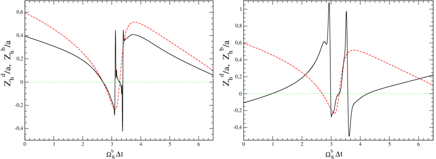
and stands for the complex conjugate. We show and the absolute value of together with Lense-Thirring frequency of a circular disc element555This is obtained from (6) by setting , and using , which corresponds the circular value of . for and , and in Fig. 1. It is seen that the curves corresponding to and are close to each other. This is because when is small, a contribution of the term proportional to to in eq. (29) plays a smaller role than the term determined by the accretion radius, which depends only on the mass ratio.
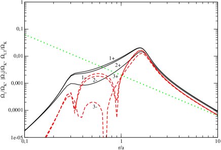
It is seen from eq. (44) that the term proportional to causes precession of a disc ring about the axis perpendicular to the orbital plane. In principal, when the second term proportional to is also taken into account, the ring dynamics could be non-trivial. As was discussed in e.g. Abod et al (2022), Aly et al (2015) and Zanazzi & Lai (2018) when precession of is solely determined by the binary, under certain circumstances, it is possible to obtain configurations of free particles and particles in a disc precessing about the direction pointing towards the periastron of the orbit. However, in our case, the Einstein precession of appears to be much faster than the one determined by the binary. The term proportional to in this situation is averaged out and causes little effect on the evolution of our system, see below.
3.1.1 Expressions for and in asymptotic limits and
In both limits and , it is easy to evaluate and analytically. For that, we note that in these limits we can set and that the integral defined in (35) is approximately equal to in both limits. Using these facts, it can be shown that integrals entering (41) are elementary when and they can be shown to be reduced to Legendre polynomials of when . In the first case, we obtain
| (46) |
while in the second case, we have
| (47) |
Substituting these expressions in (42) we obtain
| (48) |
when and
| (49) |
when .
3.2 The rate of apsidal precession
In order to calculate the apsidal advance rate, , at first we calculate the angular frequency of circular motion, perturbed by the presence of the companion, , according to the relation
| (50) |
and epicyclic frequency, , which follows from the relation
| (51) |
Then, the apsidal advance rate is determined by their difference, . Assuming that the perturbing potential is small in absolute value, we can easily obtain
| (52) |
where the bar stands again for the double average over the azimuthal angle and the orbit.
For our purposes, it is sufficient to use in (52) the doubly averaged value of the perturbing potential in the orbital plane (32). Thus, we neglect any contribution to the apsidal advance rate due to the difference between orbital plane and the plane of the disc. This value can be represented in the form
| (53) |
where is given in (35).
Note that we assume that the disc material always moves in the positive direction, while the motion of the perturber can be both in positive and negative directions. In the latter case, (52) should be multiplied by minus.
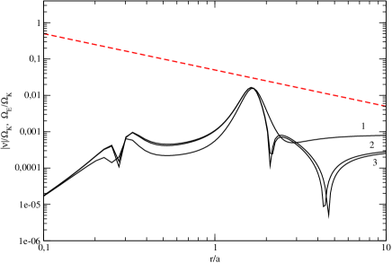
We show the absolute value of in Fig. 2 for , and , and together with the Einstein apsidal precession frequency. It is seen that Einstein’s precession dominates at radial scales of interest. Therefore, for systems with the considered parameters, the contribution of gravitational potential of the perturber is rather insignificant.
4 Numerical and analytic analysis of the behaviour of the twisted disc in the case of relatively large viscosity
As we have mentioned above, in this Paper we consider only the discs with a relatively large viscosity, . This is because they are expected to evolve in manner, which is qualitatively different from the low viscosity case, since their alignment time is smaller than the system life time . We also fix the orbital parameters of the binary to the values introduced above and consider two values of the binary’s inclination and .
4.1 An analytic model of the disc evolution
4.1.1 A simple qualitative analytic model
Since we are going to consider the disc at times less than , in a zero approximation, it appears to be reasonable to neglect hydrodynamical interactions in the disc at all and assume that the disc is evolving only due to the torques exerted by the binary and black hole
| (54) |
where we remind that , is the Lense-Thirring frequency and is given by eq. (44). Since depends on and as well as on and through the dependencies of the frequencies and on the disc’s Euler angles, eq. (54) is a rather complicated non-linear equation with time dependent coefficients. To make it analytically treatable, at first we average and over the angle , thus considering and set in the resulting expressions. Secondly, we neglect the term proportional to in (44). After making these simplifications, eq. (54) becomes elementary
| (55) |
with the solution
| (56) |
subject to the initial condition , where is given by (5). Equation (55) has a resonance at , such as . At radii , the assumptions leading to (55) are broken and a more accurate treatment is required, see below.
When the last term in the brackets in (56) has a large phase. Since is a function of , this leads to very sharp variations of this term over at a given time, which are supposed to be smeared out by the action of hydrodynamical interactions. We average over these variations, thus neglecting this term. In the end, we have an expression for a twisted disc, which is precessing with the Lense-Thirring frequency and is approximately stationary in the precessing frame, with the angle varying with as
| (57) |
We compare below the expression (57) with the results of numerical simulations.
4.1.2 A more accurate approach to the calculation of the quasi-stationary shape of the disc in the precessing frame
Now let us consider the disc shape near . It follows from eq. (57) that formally diverges at this radius. In order to remove this divergency, we take into account hydrodynamical interactions between the disc’s rings. For that we use an appropriate modification of the simplest form of dynamical equations describing twisted discs proposed in Demianski & Ivanov (1997), see their equations (38) and (39). Note that these equations are approximately valid in the limits and . They contain the variable and an auxiliary complex variable . Assuming that the disc is stationary in the frame precessing with Lense-Thirring frequency of the binary, , these variables can be represented as and . Instead of the last term in eq. (39) of Demianski & Ivanov (1997) we use eq. (55). In eq. (38) of Demianski & Ivanov (1997) we neglect the last term in the bracket on r.h.s, express in terms of and substitute the result in eq. (39). The resulting equation can be further simplified in a region of . We represent in this region as
| (58) |
where , and introduce two ’renormalised’ dimensionless frequencies and , according to the rule
| (59) |
It is evident from their definitions that both and do not depend on .
In this way, we obtain
| (60) |
It is easy to see from (60) that it can be reduced to a standard form of inhomogeneous Airy equation by rescaling and . Since and are proportional to they are expected to be quite large. That means that when , where is specified below, the first term on r.h.s. of (60) can be neglected and we have
| (61) |
Using (58) and (59) it is evident that (57) tends to (61) in the limit . Thus, we are looking for a solution to (60), which must tend to (61) in the case .
One can see that such a solution can be expressed in terms of Scorer’s function (see e.g. (2010) for its definition and properties) of a complex argument
| (62) |
Note that admits the integral representation (e.g. (2010))
| (63) |
which allows for a very efficient numerical evaluation of (62). The scale can be defined by the condition that the absolute value of the argument in (62) is equal to one. From that we have .
Now we change the dependent variable in (62) to , where and are understood to be functions of an arbitrary . When by its construction. The expression
| (64) |
is reduced to (62) when and it is reduced to (57) when . It provides an approximate analytic solution to our problem valid for any value of radius. We compare our analytic expression (64) with the results of our numerical work below, see Section 4.2.3.
4.2 Numerical calculations
4.2.1 Specific details of our numerical approach
The hydrodynamical model of a twisted disc which includes the gravitomagnetic action of the primary black hole is considered here employing the dynamical equations derived in Zhuravlev & Ivanov (2011). The equations (60-61) of Zhuravlev & Ivanov (2011) describe the geometrically thin relativistic accretion disc around a slowly rotating black hole. These equations are linear with respect to the disc inclination angle and based on the background model of the vertically isothermal flat disc as introduced by the Novikov-Thorne solution. It is assumed that the disc aspect ratio is determined by the Thomson scattering, which yields its profile according to equation (37) of Zhuravlev & Ivanov (2011). In the results shown below, it is assumed that the characteristic aspect ratio entering equation (37) of Zhuravlev & Ivanov (2011), . The standard form of the viscosity prescription is given by (35) of Zhuravlev & Ivanov (2011), which introduces the dimensionless viscosity parameter .
In this Paper, we incorporate the new terms entering the right-hand side of equation (44) into the right-hand side of the twist equation (61) of Zhuravlev & Ivanov (2011). Also, the correction to epicyclic frequency due to the gravitational influence of the secondary black hole, see equation (52), is taken into account in equation (60) of Zhuravlev & Ivanov (2011), which describes the velocity perturbations induced by the disc twist.
The dynamical equations generalised in this way are numerically advanced using an explicit second-order scheme. The dynamical variables and 666These notations are taken from Zhuravlev & Ivanov (2011), the variable is related to the variable introduced in Demianski & Ivanov (1997) and discussed in Section 4.1.2. In particular, we have far from the black hole. are set on the spatial grids uniform in with the grid nodes for shifted with respect to the grid nodes for by a half step. The quantities , and representing the influence of the pertuber are tabulated first on the separate three-dimensional mesh of its arguments, which are , and . Next, they are evaluated in the grid nodes of the scheme by the successive linear interpolations along , and . Since the disc shape and the binary orbit evolve, this procedure is repeated at each slice. The time step is limited by a value inverse to the largest absolute value of the frequency being the solution to local dispersion relation derived from the dynamical equations. We performed additional tests of the scheme in order to check that the convergence of the numerical solution is achieved for the case and, additionally, for . For that, the spatial grid step must be significantly smaller than the disc thickness in the vicinity of the inner boundary in the case . However, it may even exceed the inner disc thickness in the case . Thus, we find that the case of smaller viscosity is far more demanding for the scheme. The regularity boundary conditions, and , are imposed close to the inner boundary of the disc, where the surface density of the standard accretion disc vanishes. Note that in the limit of slow primary black hole rotation, the inner boundary of a twisted disc is formally set to its Schwarzschild value, , see the analysis in Zhuravlev & Ivanov (2011).
4.2.2 Results of numerical calculations of the case with
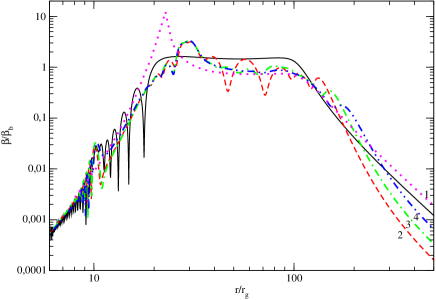
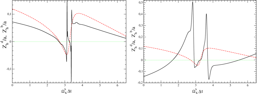
We consider numerical runs with , and . We evolve all runs up to the end times order of or larger than the evolution time .
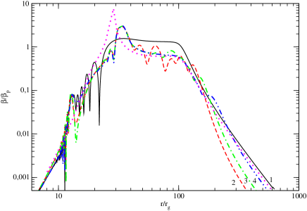
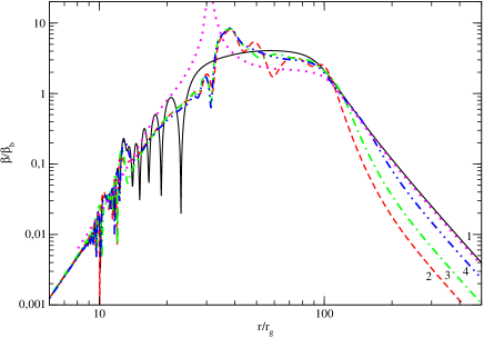
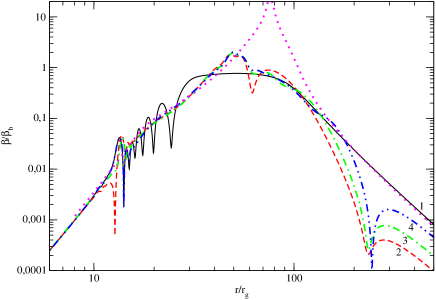
In Figs.3 and 4 we show ratios on for different times , for the case , for and , respectively. Solid (labeled as 1), dashed (labeled as 2), dot dashed (labeled as 3) and dot dot dashed (labeled as 4) curves correspond to , , and , respectively. Note that all labels are always in the bottom right corner, the label 1 is always slightly above the corresponding curve, while all other labels are slightly below.
One can see from these Figs. that the distribution of the disc inclination angle relaxes in a relatively short time to a quasi-stationary shape. The simple analytic expression (57) shown by the dotted curve describes rather well this distribution apart from the region, where is close to its maximal value and as expected. The agreement is better for the prograde black hole rotation and smaller .
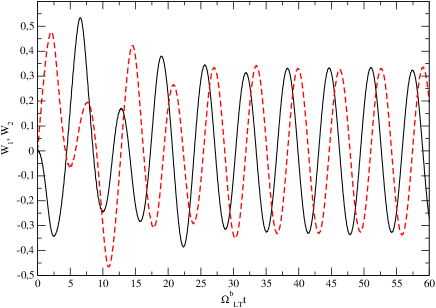
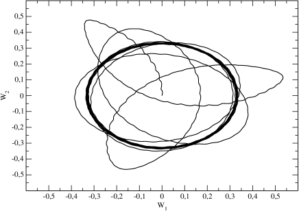
The dependency of and at the radius on time in units of the inverse Lense-Thirring frequency of the binary is shown in the left panel of Fig. 5, while the corresponding evolutionary track on the plane is shown on the right panel of the same Fig. One can see that at sufficiently large values of the evolution is practically harmonic, with the phase of differing from that of by and the time period approximately equal to . We have checked that the same type of evolution is observed for other radii and other calculation parameters. This confirms that the disc is indeed precessing with its precessional frequency equal to the Lense-Thirring frequency of the binary as suggested by our analytic model.

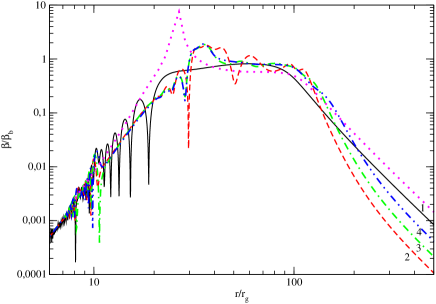
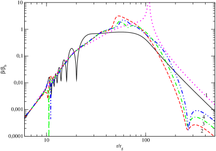
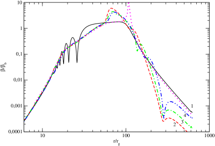
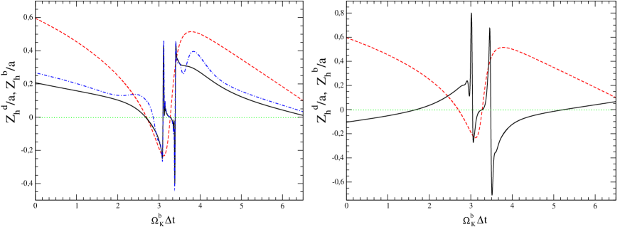
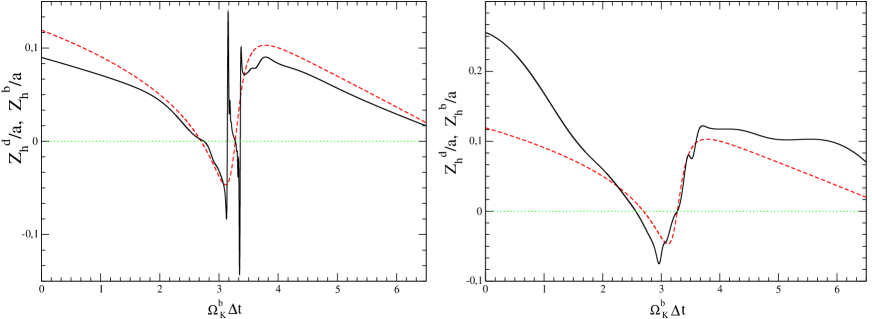
The case is qualitatively similar to the case . Therefore, we show only the dependencies of on for particular moments of time together with the analytical curves represented again by dotted lines. These are shown in Figs. 6 and 7, which are analogous to Figs. 3 and 4. As seen from these figures, the agreement between analytical and numerical results looks slightly better for the smaller absolute value of .
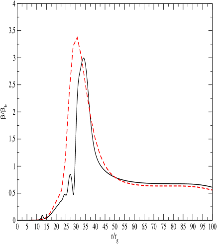
4.2.3 A more detailed comparison of our analytic and numerical results
Since the expression for given by equation (45) depends both on and the angle , in order to compare our results with the analytic expression (64), we remind that we average numerically calculated profiles of over this angle in order to obtain entering (64). We use the case and for the comparison, the result is shown in Fig. 8 for the case together with the corresponding result of numerical computation taken at some late computational time when the numerical distribution of is almost stationary. As seen from this figure, the numerical and analytic curves almost coincide at radii larger than the radii corresponding to the maximum of . These maximal values agree with the accuracy order of 10 per cent. Also, the radius corresponding to the maximum value of the analytic curve is shifted towards smaller values of by the same amount. Overall, we see that our rather simple analytic approach gives quite a reasonable approximation to the numerical result.
4.3 The influence of the disc tilt and twist on timing of intersections between the perturber and the disc
Now let us briefly consider how possible conditions of the intersections between the perturber and the disc are modified by the presence of the disc’s tilt and twist. For that, we look for the intersections of the disc by the pertuber by comparing the vertical coordinate of the perturber in the coordinate system associated with the primary, , calculated along its orbit, with the corresponding height of the disc, . is strictly defined as the vertical coordinate of a point on the disc belonging to the line perpendicular to the equatorial plane, which crosses the orbit at the point with the coordinate . Since both quantities are taken along the orbit, it is clear that the perturber crosses the disc when and only when . It is also evident that when the disc is flat the condition of intersection is just .
The instant location of the perturber with respect to the ascending node of its orbit is evaluated as , where is the current true anomaly of the perturber. The latter is determined numerically employing an iterative solution of the Keplerian equation (16) and the standard relation between the true and the eccentric anomalies. We assume below that , and that corresponds to the passage of periastron. In the linear approximation over the angle , we have
| (65) |
where is the current distance between the holes.
Similarly, in the linear approximation over , we have
| (66) |
where is the position angle of the disc element located above (or below) the perturber with respect to the ascending node of the disc ring specified by the angles and . In the same approximation we can use
| (67) |
which determines together with equation (66).
and are shown for a particular orbital period in Figs. (9-13). The instant values of and are obtained according to the uniform apsidal and nodal precessions of the binary orbit with the frequencies and , respectively, assuming that and . For our orbital parameters, it gives the minimal time interval of the order of one year between the successive intersections of the disc in the flat disc case, which is broadly consistent with the PM model of OJ 287. Since we are going to discuss only the principal importance of the disc tilt and twist, this appears to be sufficient for our study.
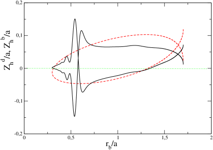
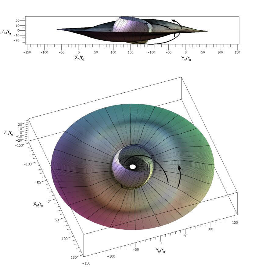
In Figs. 9 we show the dependencies of and on time during one orbital period, for the disc model with and evolved for a sufficiently long time to the quasi-stationary state. We see that both the number of crossings and the time passed between particular crossings of the disc differ very significantly from the flat disc case. Formally, we have six crossings of the disc instead of two in the flat case. Note, however, that certain crossings happen very close to each other, as e.g. the ones close to in the prograde case, these particular pairs could merge if we take into account e.g. the finite thickness of the disc or the fact that the perturber is expected to expel the disc material within its accretion radius from the orbit. We further illustrate this case in Fig. 10 showing the evolution of and on the plane , where is the distance from the primary. One can see from this figure that the section of this disc has rather non-trivial from, with a ’butterfly-like’ feature close to . This feature is explained using the results of Section 4.1. From these results it follows that close to the resonance radius the disc’s nodal angle rotates by . The same effect is also observed in our numerical calculations. This rotation leads to a very sharp variation of the disc height along the orbit when the perturber’s distance is close to .
We confirm that our main conclusion that the number of disc’s crossings per period is significantly modified is robust in Figs. 11-13. In Fig. 11 we illustrate the case with the same value of black hole rotational parameter , but for the orbit with , while in Fig. 12 and 13 we show the results for the case , for and , respectively. One can see that the qualitative situation remains the same, although the numbers of crossings and the crossing times differ from case to case. Additionally, on the left panel of Fig. 11 we show the case of a disc model with the same parameters, but with set artificially to zero. This corresponds to averaging of our disc model over a time period order of . It is seen again that that the situation remains very similar to the general case.
Finally, in Fig. 14 we show a three-dimensional picture of the disc, the perturber’s orbit and their intersections. One can clearly see a ’spiral rim’ at radii close to the resonance radius in this Fig.
5 Conclusions and Discussion
In this Paper we considered effects caused by interaction of an eccentric inclined binary black hole with a very thin () accretion disc. The orbital parameters of the binary were assumed to be the same as in the so-called ’precessing massive’ (PM) model of OJ 287 (see e.g. Valtonen et al (2023) and references therein). Namely, it was assumed that the binary consists of two black holes with masses and on a very eccentric orbit with eccentricity and the semi-major axis corresponding to the orbital period in the observer’s frame . A distinctive feature of such a system is that its evolution time due to the emission of gravitational waves is smaller than the disc relaxation time , which suggests that the disc is unable to react to the presence of the binary by e.g. opening a gap inside its orbit. Moreover, when the disc viscosity parameter , the evolution time is smaller than the time associated with alignment of the disc to a quasi-stationary twisted configuration. It is this case that has been studied in this Paper in some detail.
We calculated the torque exerted on the disc by an inclined binary, assuming that the mass ratio is small and one can use a perturbation theory. Technically, we double averaged the expression for the gravitational force responsible for this torque over the binary period and over a period of a particular disc element on a slightly perturbed circular orbit. The same procedure is used to obtain a correction to the apsidal precession rate of the disc elements. We assumed that the double averaging procedure can be used to describe the evolution of the disc over characteristic time exceeding the binary orbital period and typical orbital periods of the disc elements. It was also assumed that the perturbing component does not produce torques on the disc inside its ’accretion radius’, since gas inside this radius is likely to be removed from the system. In general, the corresponding torque and the apsidal precession rate are obtained numerically, but simple asymptotic expressions can be found for the disc’s elements with radii much smaller or much larger than . We have checked that these expressions agree with similar expressions obtained in other studies.
We used the torque term and the apsidal precession rate together with the standard expressions for these quantities induced by a relatively slowly rotating central black hole (primary) to calculate numerically the evolution of the disc tilt and twist from the flat configuration initially aligned with the equatorial plane of the primary. We set for our runs and used four values of the primary rotational parameter and , where the plus (minus) sign corresponds to prograde (retrograde ) rotation of the primary with respect to the direction of motion of the disc’s elements. We found that in all cases the disc relaxes to a non-trivial quasi-stationary configuration in the frame rotating with the Lense-Thirring frequency of the orbit . The corresponding relaxation time of the order of the corresponding period is much smaller than . After the period of relaxation, the disc’s inclination angle is almost stationary at scales order of . It is shown that significantly varies inside the orbit. When , its value in the vicinity of its periastron is much smaller than the orbital inclination angle . At radii between the periastron and apoastron of the orbit, becomes a few times larger than while approaching back to in the vicinity of apoastron.
Our preliminary analysis of the conditions of the crossing times made in Section 4.3 shows that there are, in general, more intersections of the perturber with the twisted disc per one orbital period that in the flat disc case. This happens in part due to the large disc’s tilt at scales of the order of the perturber’s orbit, and, in part, due to a large disc’s twist near ’resonance’ radius , where the precession frequency of a disc element both due to the actions of the binary and the primary coincides with . Close to this resonance the disc’s nodal angle rotates by . Clearly, our results must be taken into account in the modelling of OJ 287 and similar sources.
In Section 4.1.1 we proposed an elementary analytic model for the distribution of the disc inclination over , which agrees with the numerical results surprisingly well apart from scales close to . A more accurate, albeit more involved treatment was considered in Section 4.1.2. It describes the quasi-stationary shape of the disc in the frame precessing with the Lense-Thirring frequency of the binary at all radii, including the ones close to the resonance. We compared the analytic and numerical results in Section 4.2.3, and showed that those are in good agreement. It is important to stress that one of the reasons of the agreement is that the term proportional to in (44) is not very important. It is proportional to , and evolves on a relatively fast timescale of Einstein’s apsidal precession. However, the disc tilt and twist mainly evolve on a longer timescale order of , so that a contribution of the term proportional to is averaged out. Therefore, we can assume that the timescale of averaging the potential perturbations in Section 3 can be shorter than, but of the order of .
Our analytic results can be helpful in calculating some approximate shapes of the disc without the use of numerical integration of the equations for the disc’s tilt and twist for other parameters of the system. For that, one can numerically evaluate the distribution of using the results obtained in Section 3.1 for any desired parameters of the binary and the disc and use results of Section 4.1 to find the disc shape. This approach can, for example, be used in an accurate modelling of light curves of OJ 287 in the framework of the PM model, allowing for the possibility of multiple disc crossings per orbital period found in this work. Of course, our approach is valid only for systems with sufficiently large values of .
In this Paper we did not make attempts to compare our model with observations. This requires a detailed survey of the parameter space which deserves a separate study with careful consideration of a lot of other factors influencing the determination of the light curve (see Dey et al (2018) and Zwick & Mayer (2023) for a state-of-the-art modelling of the timing of OJ287 flares). Note, however, that it seems to be clear that taking into account of our results may lead to a significant revision of the parameters of the system in the framework of PM model. Alternatively, it can provide arguments in favour of other models, such as the models based on the jet activity (e.g. Britzen et al (2023)) or, for example, the models of eccentric binary black holes of comparable masses immersed in a circumbinary disc, e.g. Hayasaki, Mineshige & Sudou (2007) and Hayasaki, Mineshige & Ho (2008).
The numerical calculations should also be extended to smaller values of . As we briefly discussed in the text, smaller values of turn out to be demanding from the numerical point of view, and, therefore, numerical simulations of the discs with lower viscosity are left for a future work. It is interesting to mention that the low viscosity discs can, in principle, have a qualitatively different behaviour. Namely, the presence of the resonance discussed in Section 4.1 suggests a possibility of launching warp waves near the resonance by a mechanism similar to the well-known Goldreich & Tremaine (1979) mechanism of launching density waves near Lindblad resonances. This problem is beyond the scope of this work and is left for the future.
Of course, our model should be checked with either SPH or grid based three-dimensional simulations. For that, one does not need to consider very thin discs or very long simulation times. It would suffice to check whether our expression for the binary torque term is valid considering thicker discs on time scales of several .
Finally, it is interesting to find out how systems with the assumed parameters of OJ 287 can, in principle, be formed? In this connection we would like to propose the following scenario. It is known that outside the radius of influence of the more massive black hole the effects of dynamical friction could lead to the formation of a quite elongated orbit of the perturber under certain conditions (see e.g. Polnarev & Rees (1994) for analytic results and Quinlan & Hernquist (1997) for numerical experiments). Assuming that these conditions are fulfilled, a characteristic time of a significant change in orbital angular momentum due to gravitational scattering of stars of the central cluster is smaller than that of a significant change in the orbital size. In the course of the orbital evolution, the angular momentum could acquire very small values corresponding to impact parameters order of hundreds of gravitational radii of the primary black hole. In this situation, the process of direct capture of the perturber onto a bound orbit due to emission of gravitational waves is possible and a simple estimate shows that this effect may be realistic for systems with parameters appropriate to those required in galactic centres harbouring black holes as massive as . To the best of our knowledge, such a scenario has not yet been considered. Its analysis is left for a future work.
Acknowledgments
VVZ acknowledges the support of Roscosmos. We are grateful to P. C. Fragile, K. Hayasaki, J. C. B. Papaloizou and E. A. Vasiliev for useful comments, K. Zhuravleva for help and the referee for a very helpful report.
6 DATA AVAILABILITY
There are no new data associated with this article.
References
- Abod et al (2022) Abod, C. P., Chen, C., Smallwood, J., Rabago, I, Martin, R. G., Lubow, S. H., 2022 MNRAS, 517, 732
- Aly et al (2015) Aly, H., Dehnen, W., Nixon, C., King, A., 2015, MNRAS, 449, 65 MNRAS, 517, 732
- Artymowicz (1994) Artymowicz, P., 1994, ApJ, 423, 581
- Artymowicz & Lubow (1994) Artymowicz, P., Lubow, S. H., 1994, ApJ, 421, 651
- Britzen et al (2023) Britzen, S., Zajacek, M., Gopal-Krishna, Fendt, C., Kun, E., Jaron, F., Sillanpää, A., Eckart, A., 2023, ApJ, l, 951, 106
- Demianski & Ivanov (1997) Demianski, M., Ivanov, P. B., 1997, AA, 324, 829
- Dey et al (2018) Dey, L. at al, 2018, ApJ, 866, 11
- Dogan et al (2015) Dogan, S., Nixon, C., King, A., Price, D.J., 2015, MNRAS, 449, 1251
- Dotti, Sesana & Decarli (2012) Dotti, M., Sesana, A., Decarli, R., 2021, Advances in Astronomy, 2012, 940568
- Eracleous et al (2012) Eracleous, M., Boroson, T. A., Halpern, J. P., Liu, J., 2012, ApJ Suppl, 201, 23
- Ferrarese & Ford (2005) Ferrarese, L., Ford, H., 2005, Space Science Reviews, 116, 523
- Graham et al (2015) Graham, M. J., Djorgovski, S. G., Stern, D., Drake, A. J., Mahabal, A. A., Donalek, C., Glikman, E., Larson, S., Christensen, E., 2015, MNRAS, 453, 1562
- Goldreich & Tremaine (1979) Goldreich, P., Tremaine, S., 1979, ApJ, 233, 857
- Gurkan & Hopman (2007) Gurkan, M. A., Hopman, C., MNRAS, 379, 1083
- Hayasaki, Mineshige & Sudou (2007) Hayasaki, K., Mineshige, S., Sudou, H., 2007, Publ. Astron. Soc. Japan, 59, 427
- Hayasaki, Mineshige & Ho (2008) Hayasaki, K., Mineshige, S., Ho, L. C., 2008, ApJ, 682, 1134
- Hayasaki, Saito & Mineshige (2013) Hayasaki, K., Saito, H., Mineshige, S., 2013, Publ. Astron. Soc. Japan, 65, 86
- Hayasaki et al (2015) Hayasaki, K., Sohn, B. W., Okazaki, A. T., Jung, T., Zhao, G., Naito, T., 2015, JCAP, 07, 005
- Hourigan & Ward (1984) Hourigan, K., Ward, W. R., 1984, Icarus, 60, 29
- Ivanov & Illarionov (1997) Ivanov, P. B., Illarionov, A. F. 1997, MNRAS, 285, 394
- Ivanov, Igumenshchev & Novikov (1998) Ivanov, P. B., Igumenshchev, I. V., Novikov, I. D., 1998, ApJ , 507, 131
- Ivanov, Papaloizou & Polnarev (1999) Ivanov, P. B., Papaloizou, J. C. B., Polnarev, A. G., 1999, MNRAS, 307, 79
- Komossa et al (2023) Komossa, S., Grupe, D., Kraus, A., Gurwell, M. A., Haiman, Z., Liu, F. K., Tchekhovskoy, A., Gallo, L. C., Berton, M., Blandford, R., Gómez, J. L., Gonzalez, A. G., 2023, MNRAS, 522, L84
- Komossa (2006) Komossa, S., 2006, Memorie della Società Astronomica Italiana, 77, 733
- Lin & Papaloizou (1986) Lin, D. N. C., Papaloizou, J. C. B., 1986, ApJ, 309, 846
- Larwood & Papaloizou (1997) Larwood, J. D., Papaloizou, J. C. B., 1997, MNRAS, 285, 288
- Lehto & Valtonen (1996) Lehto, H. J., Valtonen, M. J., 1996 ApJ, 460, 207
- Malik et al (2015) Malik, M, Meru, F., Mayer, L., Meyer, M., 2015, ApJ, 802, 56
- Malinovsky & Mikheeva (2023) Malinovsky, A. M., Mikheeva, E. V., Astronomy Reports, 67, 685
- Meritt (2013) Meritt, D., 2013, in Dynamics and Evolution of Galactic Nuclei. Princeton, NJ: Princeton University Press
- Morales & Teixeira et al (2014) Morales Teixeira D., Fragile P. C., Zhuravlev V. V., Ivanov P. B., 2014, ApJ, 796, 103
- (32) Novikov, I. D., Thorne, K. 1973, in Black Holes, ed. C. DeWitt B. DeWitt (New York: Gordon and Breach), 343
- (33) Ogilvie, G. I., 1999, MNRAS, 304, 557
- (34) Ogilvie, G. I., 2006, MNRAS, 365, 977
- (35) Ogilvie, G. I., Latter, H. N., 2013, MNRAS, 433, 2403
- (36) Olver, F. W. J., Lozier, D., M., Boisvert, R. F., Clark, C. W., 2010, NIST Handbook of Mathematical Functions, Cambridge University Press
- (37) Papaloizou J. C. B., Pringle J. E., 1983, MNRAS, 202, 1181
- (38) Peters, P. C., 1964, Physical Review, 136, 1224
- (39) Petterson, J. A., ApJ 226, 253, 1978
- Polnarev & Rees (1994) Polnarev, A. G., Rees, M. J., 1994, AA, 283, 301
- Quinlan & Hernquist (1997) Quinlan, G. D., Hernquist, L., 1997, New Astron., 2, 533
- Rauch & Tremaine (1996) Rauch K. P., Tremaine S., 1996, New Astron., 1, 149
- Shakura & Sunyaev (1973) Shakura, N. I., Sunyaev, R. A., 1973, AA, 24, 337
- Sillanpaa et al (1988) Sillanpaa, A., Haarala, S., Valtonen, M. J., Sundelius, B., Byrd, G. G., 1988, ApJ, 325, 628
- Valtonen et al (2008) Valtonen, M. J., Lehto, H. J., Nilsson, K., Heidt, J., Takalo, L. O., Sillanpaa, A., Villforth, C., Kidger, M., Poyner, G., Pursimo, T., Zola, S., Wu, J. -H., Zhou, X., Sadakane, K., Drozdz, M., Koziel, D., Marchev, D., Ogloza, W., Porowski, C., Siwak, M. 2008, Nature, Nature, 452, 851
- Valtonen et al (2023) Valtonen, M. J., Zola, S., Gopakumar, A., Lahteenmaki, A., Tornikoski, M., Dey, L. , Gupta, A. C., Pursimo, T., Knudstrup, E., Gomez, J. L., Hudec, R., Jelinek, M., Strobl, J., Berdyugin, A. V., Ciprini, S., Reichart, D. E., Kouprianov, V. V., Matsumoto, K., Drozdz, M., Mugrauer, M., Sadun, A., Zejmo, M., Sillanpaa, A., Lehto, H. J., Nilsson, K., Imazawa, R., Uemura M., 2023, MNRAS 521, 6143
- Xiang-Gruess & Papaloizou (2014) Xiang-Gruess, M., Papaloizou, J. C. B., 2014, MNRAS, 440, 1179
- Young et al (2023) Young, A. K., Stevenson, S., Nixon, C. J., Rice, K., MNRAS, Advance Access
- Zanazzi & Lai (2018) Zanazzi, J. J., Lai, D., 2018, MNRAS 473, 603
- Zhuravlev & Ivanov (2011) Zhuravlev, V. V., Ivanov, P. B., 2011, MNRAS, 415, 2122
- Zhuravlev et al (2014) Zhuravlev V. V., Ivanov P. B., Fragile P. C., Teixeira D. M., 2014, ApJ, 796, 104
- Zwick & Mayer (2023) Zwick, L., Mayer, L., 2023, MNRAS, 526, 2754