Silicon Photomultipliers for Detection of Photon Bunching Signatures

Abstract

In this work, photon bunching from LED light was observed for the first time using SiPMs. The bunching signature was observed with a significance of $7.3~{}\sigma$ using 97 hs of data. The light was spectrally filtered using a 1 nm bandpass filter and an Etalon filter to ensure temporal coherence of the field and its coherence time was measured to be $\tau_{C}=(13.0\pm 1.3)$ ps. The impact of SiPM non-idealities in these kinds of measurements is explored, and we describe the methodology to process SiPM analog waveforms and the event selection used to mitigate these non-idealities.

1 Introduction

From biomolecules to astronomical bodies, from LIDAR to Deep Space Optical communications, photon detection is a tool with wide range of scientific and technological applications. Thus, the development of new sensors enables new discoveries and pushes the frontier of knowledge in several disciplines. The ultimate photo-detector should be capable of resolving single photons with a high dynamic range, high detection efficiency and short response time, have photon-number resolution and operate at room temperature. In recent years, a novel device called Silicon Photomultiplier (SiPM) [1, 2] was developed that, in principle, fulfills all these requirements. Currently, SiPMs have been successfully implemented in medical imaging [3, 4], particle physics detectors [5, 6, 7, 8], astrophysics [9, 10] and communications applications [11, 12], among others. Nevertheless, applications to Quantum Optics and Photonics have been hindered in the past due to some of the SiPM’s non-idealities, which can be classified in two: dark counts and correlated noise. Dark counts are generated due to thermal excitation of electrons in the Silicon and so they are generated even if no light is incident on the sensors. Correlated noise has two distinct sources: crosstalk and afterpulsing. Crosstalk events occur when a primary dark or photon count produces a prompt secondary avalanche in the Silicon. Such events have an amplitude of two detected photons. In turn, afterpulsing are events in which, after a primary dark or photon count, a delayed avalanche is generated, producing two distinct events. These effects are called correlated noise because they require a primary count to appear and they degrade the sensor performance. Recently, the impact of these features in the field of quantum optics has been studied [13].

One of the landmark experiments that gave rise to the field of quantum optics was the measurement of intensity fluctuations of light detected from thermal sources, first done by Hanbury-Brown and Twiss [14]. They observed photon correlations by measuring the arrival time difference between them at two separate detectors. These correlations are referred to as HBT effect or photon bunching. Besides opening a new field of research and giving an insight into the nature of light, Hanbury-Brown and Twiss applied this technique to astronomy and used it to measure the angular diameters of several stars [15].

Nowadays, photon correlation measurements are applied to several fields, like time-correlated photon detection in time-domain diffuse optics [16], quantum version of Time-of-Flight LIDAR [17] and quantum image scanning microscopy [18]. In addition, advances in instrumentation technology have given new life to the application of the HBT technique in astrophysics. For example, the VERITAS [19] and MAGIC [20] collaborations have measured the angular diameter of various stars, and prospects for Cherenkov Telescope Array (CTA) were studied [21]. Moreover, the use of the technique was recently proposed for measuring gravitational waves [22].

In this work we demonstrate a practical use of SiPMs for Quantum Optics. We measured photon bunching from a thermal source with these novel sensors for the first time.

2 Signal-to-Noise Ratio

The usual sensors used in Quantum Optics are the avalanche photodiodes (APDs). The traditional way to measure photon bunching is to use a beamsplitter and two sensors that are triggered in coincidence [23, 24] and the time difference between photon arrivals, $dt$, is measured. In this approach, a Signal-to-Noise Ratio (SNR) can be defined as the ratio between bunched events to accidental coincidence fluctuations in a resolving time $\tau_{R}$ as [15]

$$\mathrm{SNR}_{\mathrm{APD}}=\tau_{c}\sqrt{R_{1}R_{2}}V^{2}\sqrt{\frac{T}{\tau_{R}}}\ ,$$ (1)

where $\tau_{c}$ is the coherence time of the field, $R_{i}$ is the photon rate in detector $i$, $V$ is the degree of spatial coherence, $T$ is the integration time and $\tau_{R}$ is the resolving time of the experiment. This SNR formula is valid for linearly polarized light. A time-difference histogram will have a background of accidental events and a bunching signature, centered at zero time-difference if the optical path of both sensors is the same. The background fluctuations are accidental (random) coincidences of sensor counts, which mainly come from non-correlated light. In a case where the sensor has non-negligible dark counts, like in an SiPM, these have to be taken into account. If the resolving time $\tau_{R}$ is much larger than the coherence time $\tau_{c}$, the rate of coincidences $R_{c}$ in a window of duration $\tau_{R}$ is [25, 26]

$$R_{c}=\overbrace{(R_{1}R_{2}+D_{1}D_{2})\tau_{R}}^{\text{accidental}}+\overbrace{R_{1}R_{2}\tau_{c}V^{2}}^{\text{signal}}\ ,$$ (2)

where $D_{i}$ is the Dark Count Rate (DCR) in detector $i$. From equation (2), it is possible to obtain a relation between the SNR using APDs with respect to using SiPMs as

$$\mathrm{SNR}_{\mathrm{SiPM}}=\frac{1}{\sqrt{F}}\mathrm{SNR}_{\mathrm{APD}}\ .$$ (3)

Above we defined the factor F as $F=1+\frac{D_{1}D_{2}}{R_{1}R_{2}}$, and we assumed negligible dark counts for the APD case. Equation (3) shows the impact of this non-ideality of SiPMs sensors in this kind of measurement. In addition, the ratio of bunching events to accidental events in a time $\tau_{R}$, which is calculated as $C=\frac{\tau_{c}}{\tau_{R}}V^{2}$ [25], will also decrease when comparing the APD and the SiPM cases:

$$C_{\mathrm{SiPM}}=\frac{1}{F}\frac{\tau_{c}}{\tau_{R}}V^{2}=\frac{1}{F}C_{\mathrm{APD}}\ \ .$$ (4)

It can be seen that $C_{\mathrm{SiPM}}$ and $\mathrm{SNR}_{\mathrm{SiPM}}$ approach the APD case when $F\sim 1$.

3 Experimental Setup

The experimental setup used to measure photon bunching using SiPMs is shown in Figure 1. The setup were mounted inside a light tight facility specifically designed for SiPM characterization studies [27, 28].

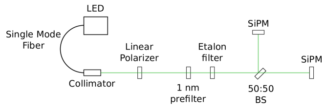
Figure 1: Schematic of the experimental setup used to detect photon bunching with SiPMs. A green LED source was coupled to a single-mode fiber to ensure spatial coherence of the field. Light was filtered with a 1 nm filter and an Etalon filter to ensure temporal coherence as well. Two 1 mm² SiPMs were placed in both arms of a 50:50 beamsplitter to perform coincidence measurements.

The light source used for the experiment was a fiber coupled LED from THOR LABS (TL M530F2) with a center wavelength of 530 nm. Its output was fed into a single mode optical fiber, which is used to enforce spatial coherence of the field. A rate of $10^{10}$ photons per second was obtained at the output of the fiber collimator. A linear polarizer was placed in the beam path. Then, to increase the coherence time of the field, light was spectrally filtered using a 1 nm FWHM filter (TL FL05532-1) and an etalon filter (Light Machinery, OP-7423-1686-1). The etalon free spectral range is such that approximately 17 peaks fall in the 1 nm FWHM optical passband of the interference filter [29]. The coherence time of this configuration was estimated to be of the order of 10 ps [25]. Finally, the beam was separated with 50:50 beamsplitter and both SiPMs were placed at the same distance from it. Each SiPM (ONSEMI MicroFC-10035-SMT) was connected to an Analog Front-End board designed in-house with a time resolution below 1 ns. SiPMs were biased at 5 V overvoltage using a SourceMeter Unit and the SiPM DC current was monitored during the whole experiment. No temperature control on them was performed, but the experiment room was kept at $(22\pm 1)$ ^oC. SiPMs were both placed at a distance of $(85\pm 1)$ cm from the collimator output. SiPM analog waveforms were acquired using a digitizer at 500 MSps (PicoScope 2406B) and the coincidence window used was 100 ns. A 3 ns cable delay was placed in one of the SiPM channels to help rule out hardware glitches.

Two experiments were performed: First, a signal measurement where the field was both spatially and temporally coherent (and thus bunching could be observed). Then, a background measurement where the effect was not present, because the field was purposely not temporally coherent. To remove the temporal coherence of the field, the 1 nm filter and the Etalon filter were removed and replaced with an optical attenuator to avoid SiPM signal saturation. In the case where photon bunching is not present, the background is expected to be uniform at short times.

The DCR and the detected photon rate on each SiPM for both experiments is shown in Table 1.

SiPM	DCR [kcps]	Signal experiment rate [kcps]	Bkgnd. experiment rate [kcps]
1	126 $\pm$ 1	629 $\pm$ 1	517 $\pm$ 1
2	148 $\pm$ 1	446 $\pm$ 1	522 $\pm$ 1

Table 1: SiPM parameters and rates for signal and background experiments.

The measured coincidence rate between the two detectors in the 100 ns coincidence gate was about 10 kcps. Considering the acquisition dead time, both signal and background experiments were run for an effective time of 97 hs. Using equation (3), the expected SNR for that effective acquisition time is 96.

4 Event Selection

For each event, several parameters were calculated from the digitized waveforms acquired. These parameters were: the Baseline average and its standard deviation, Trigger Timestamp, Time-over-Threshold (ToT), waveform Amplitude, and waveform Maximum and Minimum values. These parameters were used for posterior event selection. An example of an acquired event can be seen in Figure 2.

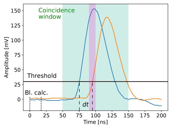
Figure 2: Example of an acquired event. The coincidence window of 100 ns is shown in green and the threshold for Timestamp determination is shown in black. The time difference between events, $dt$, in both SiPMs is shown as well. The Baseline level (Bl) was determined using the first 16 ns of each waveform. An additional window of 10 ns width and centered in 95 ns, which was used for posterior data selection, is shown in violet.

All parameters were calculated using digital pulse processing. To determine the Baseline mean and its standard deviation, the first 16 ns of each event were used. The Timestamp of the detected photon was determined using a linear interpolation of the waveform and a software leading-edge discriminator. The Threshold used for the discriminator was set 30 mV over the previously calculated Baseline level. To calculate the signal ToT, a falling-edge discriminator was used to obtain the second intercept between the waveform and the Threshold. The ToT was obtained as the difference between the Trigger Timestamp and the falling edge intercept. The waveform Amplitude was calculated as the waveform Maximum minus the Baseline level.

Only events with the following properties were accepted to be included in the time-difference histogram:

1. Baseline standard deviation lower than 4 mV. This selection cut removes events with noisy or fluctuating baselines. An unstable baseline degrades the time resolution of the Trigger Timestamp determination.

2. At least one of the Trigger Timestamps present inside a 10 ns window centered at 95 ns. Due to the way the digitizer acquisition was configured, at least one of the channel triggers is expected inside this window. This selection window is shown in violet in Figure 2.

3. No trigger timestamps present inside the baseline calculation samples.

4. Events with $\mathrm{ToT}<80$ ns. Large values of ToT indicate a spurious pile-up event and were rejected.

5. Waveforms with an amplitude less than 200 mV. This selects events with only one detected photon -or dark count-. This removes events with crosstalk or events with two coincident photon detections on the same SiPM.

5 Results and Discussion

After event selection, the time-difference histogram was constructed for the two experiments performed. On both histograms, an unwanted sinusoidal-like systematic pattern with a period of 2 ns was observed. The reason for this effect is that the digitizer-board channels are only synchronized down to its sampling period of 2 ns. The top histogram of Figure 3 shows the raw data points with this structure. The amplitude of this electronic jitter is negligible compared to the mean entry number, but relevant for observing the bunching peak. Due to this, a procedure had to be devised to remove this systematic effect. First, the time-difference histogram of the background dataset was cut into 2 ns slices. Then, all these slices were folded together and averaged into a single 2-ns window, where random noise was mitigated. This 2 ns window was then repeated along the time-difference axis to build a template of the systematic structure. This template was then used to normalize the raw histogram, and it is shown on the top plot of Figure 3. On the bottom plot of that same figure, the normalized histogram is shown. A uniform fit was performed on the normalized background with a resulting $\chi^{2}/\mathrm{dof}=99.7/100$ and a p-value of 0.49. In addition, a Kolmogorov-Smirnoff (KS) test [30] was run to compare the background to a uniform distribution, and a p-value of 0.37 was obtained. Both tests are consistent with the expected background distribution in the absence of bunching signatures.

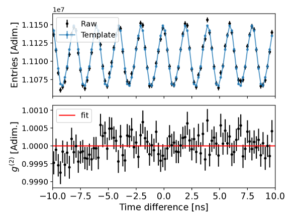
Figure 3: Top plot: raw data histogram of timestamp differences in the background experiment, along with the generated template used for the removal of the systematic 2 ns structure. Bottom plot: normalized timestamp difference histogram in the background experiment and a uniform fit with resulting $\chi^{2}/\mathrm{dof}=99.7/100$ and a p-value of 0.49.

In the signal experiment, a bunching peak is expected to appear around 3 ns, as the optical path of both sensors was the same and a cable delay was introduced in one of the channels. The top plot of Figure 4 shows the raw time-difference histogram for the signal experiment and the constructed template for the removal of the 2-ns structure. An excess of events over the template can be seen around 3 ns. As in the background case, the template was constructed slicing the raw histogram into 2-ns windows. However, two windows where the bunching peak was expected were omitted for its construction. The bottom plot of Figure 4 shows the normalized histograms for both experiments. The bunching signature can be seen over the uniform background.

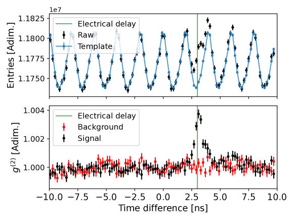
Figure 4: Top plot: raw data histogram of timestamp differences in the signal experiment, along with the generated template used for the removal of the systematic 2 ns structure. Bottom plot: normalized timestamp difference histogram of both experiments. The electrical delay of 3 ns can be seen in green.

Again, a KS test was performed against a uniform distribution on the signal time-difference histogram. The probability that the signal peak observed was caused by a background fluctuation is $10^{-14}$, which results in a significance level of $7.3~{}\sigma$.

To further identify the characteristics of the peak, a Gaussian fit was performed on it. The coherence time of the field is much smaller that the overall time resolution of the detection system, which is a combination of SiPM and electronic jitter and the digital pulse-processing algorithms. This is why the shape of the bunching peak is expected to have a Gaussian distribution [31]. Figure 5 is a zoom of the time-difference histogram centered in the bunching peak, where a Gaussian fit was performed ($\chi^{2}/\mathrm{dof}=18/16$ and $\mathrm{p-value}=0.31$).

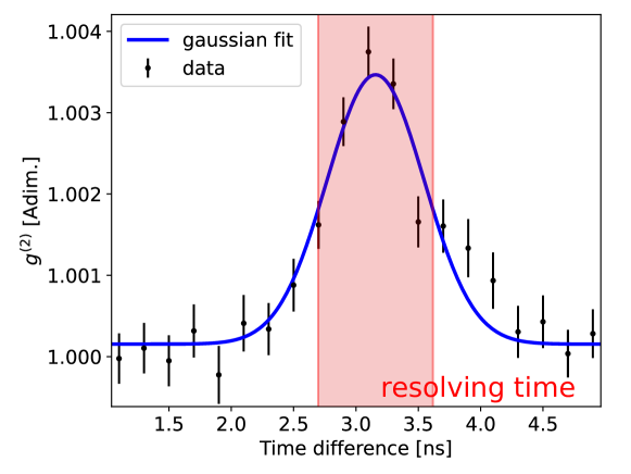
Figure 5: Signal peak with a Gaussian fit. The peak is expected to be Gaussian because it is dominated by the overall time resolution of the detection system. The fit has a $\chi^{2}/\mathrm{dof}=18/16$, which results in a $\mathrm{p-value}=0.31$. The width of the peak is $(920\pm 83)$ ps FWHM, the peak’s center is $(3.15\pm 0.03)$ ns and the peak height is $(3.3\pm 0.2)\cdot 10^{-3}$. The system resolving time, given by the composite jitter of the two SiPM detectors is shown in red (centered around the peak maximum).

The width of the Gaussian distribution obtained from the fit is $(920\pm 83)$ ps FWHM, which represents the overall time resolution of the system, or the resolving time $\tau_{R}$. The mean obtained from the fit is $(3.15\pm 0.03)$ ns, compatible with the $\sim 3$ ns cable delay introduced in one of the channels. The height obtained from the fit is $(3.3\pm 0.2)\cdot 10^{-3}$. From the latter, and using Eq. 4, the coherence time $\tau_{C}$ is $(13.0\pm 1.3)$ ps, which is consistent with the expected value of the order of 10 ps. The experimental SNR was calculated to be 99, using events in one resolving time. This value is consistent with the estimation given by equation 3.

6 Conclusions and outlook

In this work, photon bunching from LED light was measured using SiPM sensors for the first time with a 7.3 $\sigma$ significance and an SNR of 99. The coherence time of the field was measured to be $\tau_{C}=(13.0\pm 1.3)$ ps. We presented the impact of the non-idealities of SiPMs in the equations that model this phenomenon, compared to the traditional APD sensors. We described the methodology to process the analog waveform of the SiPMs, and the event selection used that mitigate the non-idealities of these sensors.

The research presented here involved an analysis of the events with an amplitude of 1 photoelectron, i.e. one detected photon or a dark count per SiPM channel. In further works, the use of the photon-number resolution of the SiPM sensor will be explored. Particularly, the impact of the correlated noise will be studied in regards to photon bunching. This analysis could open a door for observation of higher order correlations using only 2 detectors.

References

- [1] A. Otte, D. Garcia, T. Nguyen and D. Purushotham “Characterization of Three High Efficiency and Blue Sensitive Silicon Photomultipliers” In Nuclear Instruments and Methods in Physics Research Section A: Accelerators, Spectrometers, Detectors and Associated Equipment 846, 2017, pp. 106–125
- [2] A Nepomuk Otte “SiPM’s a very brief review” In International Conference on New Photo-detectors 252, 2016, pp. 001 SISSA Medialab
- [3] N. Otte et al. “The SiPM — A new Photon Detector for PET” In Nuclear Physics B - Proceedings Supplements 150, 2006, pp. 417–420
- [4] Stefan Gundacker et al. “High-frequency SiPM readout advances measured coincidence time resolution limits in TOF-PET” In Physics in Medicine & Biology 64.5, 2019, pp. 055012
- [5] Felix Sefkow, Frank Simon and CALICE collaboration “A highly granular SiPM-on-tile calorimeter prototype” In Journal of Physics: Conference Series 1162.1, 2019, pp. 012012
- [6] Babak Abi et al. “Measurement of the positive muon anomalous magnetic moment to 0.46 ppm” In Physical Review Letters 126.14, 2021, pp. 141801
- [7] M.. Mazziotta, C. Altomare and E. al. “A light tracker based on scintillating fibers with SiPM readout” In Nuclear Instruments and Methods in Physics Research Section A: Accelerators, Spectrometers, Detectors and Associated Equipment 1039, 2022, pp. 167040
- [8] V. Álvarez, M. Ball and F… al. “Design and characterization of the SiPM tracking system of NEXT-DEMO, a demonstrator prototype of the NEXT-100 experiment” In Journal of Instrumentation 8.05, 2013, pp. T05002
- [9] P Allison et al. “Cosmic-ray isotope measurements with HELIX” In Proceedings of Science 358, 2019
- [10] G. Ambrosi and V. Vagelli “Applications of silicon photomultipliers in ground-based and spaceborne high-energy astrophysics” In The European Physical Journal Plus 137, 2022, pp. 170
- [11] Long Zhang et al. “The future prospects for SiPM-based receivers for visible light communications” In Journal of Lightwave Technology 37.17, 2019, pp. 4367–4374
- [12] Zubair Ahmed et al. “A SiPM-based VLC receiver for Gigabit communication using OOK modulation” In IEEE Photonics Technology Letters 32.6, 2020, pp. 317–320
- [13] G. Chesi et al. “Optimizing Silicon photomultipliers for Quantum Optics” In Scientific Reports 9, 2019, pp. 7433
- [14] R. Hanbury Brown and R. Twiss “Correlation between Photons in two Coherent Beams of Light” In Nature 177, 1956, pp. 27–29
- [15] R. Hanbury Brown “The Intensity Interferometer” Halsted Press, 1974
- [16] A. Dalla Mora et al. “The SiPM revolution in time-domain diffuse optics” In Nuclear Instruments and Methods in Physics Research Section A: Accelerators, Spectrometers, Detectors and Associated Equipment 978, 2020, pp. 164411
- [17] P.. Tan et al. “Practical Range Sensing with Thermal Light” In Phys. Rev. Appl. 20, 2023, pp. 014060
- [18] G. Lubin et al. “Quantum correlation measurement with single photon avalanche diode arrays” In Opt. Express 27.23, 2019, pp. 32863–32882
- [19] A.. Abeysekara, W. Benbow and A. al. “Demonstration of stellar intensity interferometry with the four VERITAS telescopes” In Nature Astronomy 4, 2020, pp. 1164–1169
- [20] The MAGIC collaboration “Intensity interferometry with the MAGIC telescopes” In Proceedings of 37th International Cosmic Ray Conference 395, 2021, pp. 693
- [21] Dainis Dravins, Stephan LeBohec, Hannes Jensen and Paul D. Nuñez “Stellar intensity interferometry: Prospects for sub-milliarcsecond optical imaging” In New Astronomy Reviews 56.5, 2012, pp. 143–167 DOI: https://doi.org/10.1016/j.newar.2012.06.001
- [22] I.H. Park et al. “Stellar interferometry for gravitational waves” In Journal of Cosmology and Astroparticle Physics 2021.11, 2021, pp. 008
- [23] P.. Tan et al. “Measuting Temporal Photon Bunching in Blackbody radiation” In The Astrophysical Journal Letters 789, 2014, pp. L10
- [24] P.. Tan “Stellar Temporal Intensity Interferometry”, 2015
- [25] L. Mandel and E. Wolf “Optical Coherence and Quantum Optics” Cambridge University Press, 1995
- [26] D.. Scarl “Measurements of Photon Correlations in Partially Coherent Light” In Phys. Rev. 175, 1968, pp. 1661–1668
- [27] William Painter et al. “SiECA: Silicon photomultiplier prototype for flight with EUSO-SPB” In Proceedings of 35th International Cosmic Ray Conference 442, 2017
- [28] Max Renschler et al. “Characterization of Hamamatsu 64-channel TSV SiPMs” In Nuclear Instruments and Methods in Physics Research Section A: Accelerators, Spectrometers, Detectors and Associated Equipment 888, 2018, pp. 257–267
- [29] L.. Coldren, S.. Corzine and M.. Mašanović “Diode Lasers and Photonic Integrated Circuits” John WileySons, Inc., 2012
- [30] W.. Daniel “Applied Nonparametric Statistics” PWS-KENT Pub., 1990
- [31] M.. Nemallapudi, S. Gundacker, P. Lecoq and E. Auffray “Single photon time resolution of state of the art SiPMs” In Journal of Instrumentation 11.10, 2016, pp. P10016