BRAU-Net++: U-Shaped Hybrid CNN-Transformer Network for Medical Image Segmentation

Abstract

Accurate medical image segmentation is essential for clinical quantification, disease diagnosis, treatment planning and many other applications. Both convolution-based and transformer-based u-shaped architectures have made significant success in various medical image segmentation tasks. The former can efficiently learn local information of images while requiring much more image-specific inductive biases inherent to convolution operation. The latter can effectively capture long-range dependency at different feature scales using self-attention, whereas it typically encounters the challenges of quadratic compute and memory requirements with sequence length increasing. To address this problem, through integrating the merits of these two paradigms in a well-designed u-shaped architecture, we propose a hybrid yet effective CNN-Transformer network, named BRAU-Net++, for an accurate medical image segmentation task. Specifically, BRAU-Net++ uses bi-level routing attention as the core building block to design our u-shaped encoder-decoder structure, in which both encoder and decoder are hierarchically constructed, so as to learn global semantic information while reducing computational complexity. Furthermore, this network restructures skip connection by incorporating channel-spatial attention which adopts convolution operations, aiming to minimize local spatial information loss and amplify global dimension-interaction of multi-scale features. Extensive experiments on three public benchmark datasets demonstrate that our proposed approach surpasses other state-of-the-art methods including its baseline: BRAU-Net under almost all evaluation metrics. We achieve the average Dice-Similarity Coefficient (DSC) of 82.47, 90.10, and 92.94 on Synapse multi-organ segmentation, ISIC-2018 Challenge, and CVC-ClinicDB, as well as the mIoU of 84.01 and 88.17 on ISIC-2018 Challenge and CVC-ClinicDB, respectively. The codes will be available on GitHub.

BRAU-Net++, convolutional neural network, medical image segmentation, sparse attention, Transformer.

1 Introduction

Accurate and robust medical image segmentation plays an essential role in computer-aided diagnosis systems, especially for image-guided clinical surgery, disease diagnosis, treatment planning, and clinical quantification[1], [2], [3]. Medical image segmentation is usually considered to be essentially the same as natural image segmentation [4], and that its corresponding techniques are often derived from that of the latter [5]. Common to the two communities is that they all take extracting the accurate region of interests (ROIs) of images as a study objective in a manual or full-automatic manner. Benefiting from deep learning techniques, the segmentation task in natural image vision has achieved an impressive performance. But different from natural image segmentation, medical image segmentation demands more accurate segmentation results for ROIs, e.g., abnormalities and organs, to rapidly identify the lesion boundaries and exactly assess the level of lesion. That is because of the clinical practice that a subtle segmentation error in medical images can lead to poor user experience in clinical settings, and increase the risk in the subsequent computer-aided diagnosis [6]. Also, manually delineating the lesions and their boundaries in various imaging modalities requires extensive effort that is extremely time-consuming and even impractical, and the resulting segmentation may be influenced by the preference and expertise of clinicians [7], [45]. Thus, we believe that it is critical to develop intelligent and robust techniques to efficiently and accurately segment lesion regions or organs in medical images.

Depending on the development of deep learning as well as the extensive and promising applications, many medical image segmentation methods which rely on convolution operations have been proposed for segmenting the specific target object in medical images. Among these approaches, the u-shaped encoder-decoder architectures like U-Net [8] and fully convolutional network (FCN) [9] have become dominant in medical image segmentation. The follow-up various variants, e.g., U-Net++ [6], U-Net 3+ [10], Attention U-Net [11], 3D U-Net [12], and V-Net [13] have also been developed for image and volumetric segmentation of various medical imaging modalities, and made outstanding success in a wide range of medical applications such as cardiac segmentation, multi-organ segmentation, and polyp segmentation. The excellent performance of these CNN-based methods proves that CNN has a strong ability to learn semantic information. But it often exhibits limitations in explicitly capturing long-range dependency due to the inherent locality of convolution operations. Some studies have tried to address this problem by using atrous convolutional layers [14], [15], self-attention mechanisms [16], [17], and image pyramids [18]. However, these methods can not remarkably improve the ability to model long-range dependency.

Recently, inspired by the great success of transformer in nature language processing (NLP) [19] domain, many studies attempt to apply transformer into vision domain [20], [21], [22], [23]. These works have achieved consistent improvements on various vision tasks, which indicates that vision transformer has significant potential in the vision domain. Among these works, a popular topic is how to boost the performance of models by improving the core building block, i.e., attention. As the core building block of vision transformer, attention is a powerful tool to capture long-range dependency. However, vanilla attention is a full attention mechanism that computes pair-wise tokens affinity across all spatial locations, and thus it has a high computational complexity and incurs heavy memory footprints [24]. To alleviate the problem, some works attempt to apply sparse attention to vision transformer, in which each query token just attends to part of key and value tokens instead of the entire sequence [25]. To this end, several handcrafted sparse patterns have been explored, such as restricting attention in local windows [23], dilated windows [26], [27], or axial stripes [28]. In medical image vision community, many studies have also brought transformer into medical image segmentation task, like nnFormer [29], UTNet [30], TransUNet [1], TransCeption [3], HiFormer [32], Focal-UNet [33], and MISSFormer [34]. However, to the best of our knowledge, fewer works consider introducing sparsity thought into this field, in which the representative works involve Swin-Unet [35] and Gated Axial UNet (MedT) [36]. But these sparse attention mechanisms merge or select sparse patterns in a handcrafted manner. Thus, these patterns are query-agnostic. That is, they are shared by all queries. Applying dynamic and query-aware sparsity to medical image segmentation still remain largely unexplored.

All these problems mentioned above motivate us to explore a full-automatic advanced segmentation algorithm that can yield effective segmentation results relying on the nature of medical images, so as to benefit more image-guide medical applications. More recently, inspired by the BiFormer’s [24] success in applying sparse attention to vision transformer [37], we propose, BRAU-Net++, to leverage the power of transformer for medical image segmentation. As far as we know, BRAU-Net++ is first hybrid model that considers incorporating dynamic sparse attention into a CNN-Transformer architecture. BRAU-Net++ is also developed from BRAU-Net [38], which uses BiFormer block to build a u-shaped pure transformer network structure with skip connection for pubic symphysis-fetal head segmentation. Similar to Swin-Unet [35] and BRAU-Net [38], the main components of the network structure include encoder, bottleneck, decoder, and skip connection. The encoder, bottleneck, and decoder are all built based on the core building block of BiFormer [24]: bi-level routing attention, which effectively models long-range dependency and saves both computation and memory. Meanwhile, motivated by global attention mechanism [39], we redesign the skip connection by incorporating channel-spatial attention, which is performed through convolution operations, aiming to minimize local spatial information loss and amplify global dimension-interaction of multi-scale features. Also, similar to [24], [26], [40], [41], the proposed architecture utilizes depth-wise convolutions to implicitly encode positional information. Extensive experiments on three publicly available medical image datasets: Synapse multi-organ segmentation [56], ISIC-2018 Challenge [42], [43], and CVC-ClinicDB [44] show that the proposed method has achieved a promising performance and robust generalization ability.

Our main contributions can be summarized as follows:

1) We introduce a u-shaped hybrid CNN-Transformer network, which uses bi-level routing attention as core building block to design the encoder-decoder structure, in which both encoder and decoder are hierarchically constructed, so as to effectively learn local-global semantic information while reducing computational complexity.

2) We redesign the traditional skip connection using channel-spatial attention mechanism and propose the Skip Connection with Channel-Spatial Attention (SCCSA), aiming to enhance the cross-dimension interactions on both channel and spatial aspects and compensate the loss of spatial information caused by down-sampling.

3) We validate the effectiveness of BRAU-Net++ on three commonly used datasets: Synapse multi-organ segmentation, ISIC-2018 Challenge, and CVC-ClinicDB datasets. As a result, the proposed BRAUNet++ demonstrates a better performance than other state-of-the-art (SOTA) methods under almost all evaluation metrics.

The remainder of this paper is organized as follows. Section II reviews prior related works. Section III specifies our method, main building blocks, and training procedure. Section IV introduces our experimental settings. Section V reports the experimental details and results. Section VI gives some discussions and specifications regarding the experimental results and findings, and finally, Section VII presents our conclusion.

2 Related work

2.1 U-Shaped Architecture

2.1.1 CNN-Based U-Shaped Architecture for Medical Image Segmentation

Main techniques of this paradigm involve U-Net [8] and FCN [9], as well as subsequent variants [6], [10], [11], [12], [13], some of which are introduced into 2D or 3D medical image segmentation communities, respectively. Due to the simplicity and superior performance of the U-shaped structure, various Unet-like methods, such as U-Net++ [6], UNet 3+ [10], and DCSAU-Net [46] are constantly emerging in the field of 2D medical image segmentation. And other methods are also introduced into the field of 3D medical image segmentation, such as 3D-Unet [12] and V-Net [13]. This line of approach employs a series of convolution pooling operations to design its encoder and decoder. This paradigm has been achieved tremendous success in a wide range of medical applications due to its powerful representation ability. With respect to more works about U-Net and its variants applied for medical image segmentation, readers can refer to the related review literatures [47], [48].

2.1.2 Transformer-Based U-Shaped Architecture for Medical Image Segmentation

The original transformer architecture was first proposed for machine translation task [19], and has become the de-facto standard for natural language processing (NLP) problems. The follow-up works have made more attempts to apply transformer to computer vision. More recently, researchers have tried to develop pure transformer or hybrid transformer to perform medical image segmentation. In [35], a pure transformer, i.e., Swin-Unet, is proposed for medical image segmentation, in which the tokenized patches from raw image rather than CNN feature map, are fed into the architecture for local global semantic feature learning. In [1], a CNN-Transformer hybrid model, TransUNet, leverages both detailed high-resolution spatial information from CNN features and the global context encoded by transformers to achieve superior segmentation performance. Similar to TransUNet, UNETR [49] and Swin UNETR [50] employed transformers in the encoder and utilized a convolutional decoder to generate segmentation maps. These works use full attention or static sparse attention to compute pairwise token affinity. Different from these methods, we bring dynamic sparse attention to select most related tokens, and the input of network are the tokenized patches from raw image. Thus, the information is not lost due to lower resolution. Meanwhile, we apply convolution operation to the skip connection to enhance the global dimension-interaction of multi-scale features.

2.2 Sparse Attention Mechanism

Sparse connection patterns [37] have been introduced to address the computational and memory complexity of the vanilla attention mechanism. Sparse attention has gained more attraction in vision transformers [23], [25], [26], [27], [28]. In Swin Transformer [23], attention is constrained to non-overlapping local windows, and the shift window operation is introduced to facilitate inter-window communication among neighboring windows. Thus, this attention is handcrafted, which is based on local window. Subsequent studies have also introduced various manually designed sparse patterns, such as dilated windows [26], [27] or cross-shaped windows [31]. More recently, efficient vision transformer based on dynamic token sparsity has achieved great success. In [51], the acceleration of inference is achieved by dynamically selecting the number of tokens to be passed to the next layer through hierarchical pruning. In [25], [24], they respectively propose quad-tree attention and bi-level routing attention to achieve query-adaptive sparsity in a coarse-to-fine manner. The difference lies in the fact that bi-level routing attention aims to locate a few most relevant key-value pairs, while quad-tree attention constructs a token pyramid and assembles information from different granularity levels. In this work, we attempt to use BiFormer block as basic unit to build a u-shaped encoder-decoder architecture with SCCSA module for medical image segmentation.

2.3 Channel-Spatial Attention

Great progress has been made in the study of attention mechanism in computer vision, in which both channel attention and spatial attention are two important directions. Channel attention focuses on the information of channels in CNN. For instance, SENet [52] adaptively recalibrates the channel feature responses to enhance the discriminative ability of the network. On the other hand, spatial attention focuses on relevant spatial regions. For example, STN [53] can transform various deformation data in space and automatically capture important regional features. Building on these individual success, CBAM [54] combines channel attention and spatial attention in a concatenated manner to jointly capture complex dependencies between channels and spatial locations. Inspired by global attention mechanism [39], we use channel-spatial attention to redesign skip connection, so as to enhance channel-spatial dimension-interactive and compensate for the spatial information loss due to down-sampling.

3 Method

In this section, we start by briefly summarizing the Bi-Level Routing Attention (BRA). We then describe the overall architecture of the proposed BRAU-Net++. Finally, we introduce the BiFormer block and Skip Connection Channel-Spatial Attention module (SCCSA).

3.1 Preliminaries: Bi-Level Routing Attention

The bi-level routing attention (BRA) is a dynamic, query-aware sparse attention mechanism, whose core idea is to filter out the most semantically irrelevant key-value pairs in a coarse-grained region level, and only keep a small portion of most relevant routed regions to fine-grained token-to-token attention. Compared to other handcrafted static sparse attention mechanism [23], [31], [55], the BRA is prone to model long-range dependency. It is similar to vanilla attention on this point. But the BRA has a much lower complexity of $O((HW)^{\frac{4}{3}})$, while the vanilla attention has a complexity of $O({(HW)^{2}})$ [24].

3.1.1 Region Partition and Linear Projection

By dividing a 2D input feature map $\textbf{X}\in{\mathbb{R}^{H\times W\times C}}$ into $S$$\times$$S$ non-overlapped regions, the feature dimension ${\frac{HW}{S^{2}}}$ of each region can be obtained. Subsequently, based on the resulting feature map $\textbf{X}^{r}\in{\mathbb{R}^{{S^{2}}\times{\frac{HW}{S^{2}}}\times C}}$, the query, key, value ${\textbf{Q},\textbf{K},\textbf{V}}\in{\mathbb{R}^{{S^{2}}\times{\frac{HW}{S^{2}}}\times C}}$ can be derived by linear projections:

$$\textbf{Q}=\textbf{X}^{r}{\textbf{W}^{q}},\textbf{K}=\textbf{X}^{r}{\textbf{W}^{k}},\textbf{V}=\textbf{X}^{r}{\textbf{W}^{v}}.$$ (1)

Where ${\textbf{W}^{q}},{\textbf{W}^{k}},{\textbf{W}^{v}}\in{{\mathbb{R}}^{C\times C}}$ are linear projection weights matrix for the query, key, value, respectively.

3.1.2 Region-to-Region Routing

The process starts by calculating the average of Q and K for each region respectively, yielding region-level queries and keys, ${\textbf{Q}^{r}},{\textbf{K}^{r}}\in{{\mathbb{R}}^{{S^{2}}\times C}}$. Next, the region-to-region adjacency matrix, ${\textbf{A}^{r}}\in{{\mathbb{R}}^{{S^{2}}\times{S^{2}}}}$, is derived via applying matrix multiplication between ${\textbf{Q}^{r}}$ and transposed ${\textbf{K}^{r}}$. Finally, the key step is only keeping the top-$k$ most relevant regions for each query region via a routing index matrix, ${\textbf{I}^{r}}\in{{\mathbb{N}}^{{S^{2}}\times k}}$, with the row-wise top-$k$ operator: topkIndex(). The region-to-region routing can be formulated as:

$${\textbf{A}^{r}}={\textbf{Q}^{r}}{({\textbf{K}^{r}})^{T}}.$$ (2)

$${\textbf{I}^{r}}=\operatorname{topkIndex}({\textbf{A}^{r}}).$$ (3)

3.1.3 Token-to-Token Attention

Since the routed regions may be spatially scattered over the whole feature map, the key and value tensors in routed regions needs to be gathered. The fine-grained token-to-token attention is then applied on these key-value tensors. This process is shown in Fig. 1, and can be formulated as follows:

$${\textbf{K}^{g}}=\operatorname{gather}(\textbf{K},{\textbf{I}^{r}}),{\textbf{V}^{g}}=\operatorname{gather}(\textbf{V},{\textbf{I}^{r}}).$$ (4)

$$\textbf{O}=\operatorname{softmax}(\frac{{\textbf{Q}{{({\textbf{K}^{g}})}^{T}}}}{{\sqrt{C}}}){\textbf{V}^{g}}+\operatorname{LCE}(\textbf{V}).$$ (5)

Where ${\textbf{K}^{g}},{\textbf{V}^{g}}\in{{\mathbb{R}}^{kHW\times C}}$ are gathering key and value tensors. The function LCE(·) is parameterized using a depth-wise convolution.

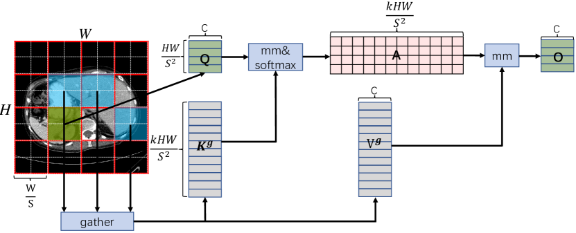
Figure 1: Illustration of token-to-token attention. By gathering the key and value tensors in routed regions, only GPU-friendly dense matrix multiplications are performed.

3.2 Architecture Overview

The overall architecture of BRAU-Net++ is shown in Fig. 2(a). The BRAU-Net++ includes encoder, decoder, bottleneck, and SCCSA module. For the encoder, given an input medical image with the size of $H\times W\times 3$, the medical image is split into overlapping patches and feature dimension of each patch is projected into arbitrary dimension (defined as C) by the patch embedding. The transformed patch tokens pass through multiple BiFormer blocks and patch merging layers to generate hierarchical feature representations. Specifically, the patch merging is used to decrease resolution of feature map and increase dimension, and the BiFormer block is used to learn feature representations. For the bottleneck, the resolution and dimension of feature map remain unchanged. Inspired by U-Net [8] and Swin-Unet [35], we design a symmetric transformer-based decoder, which is composed of BiFormer block and patch expanding layer. The patch expanding layer is responsible for up-sampling and decreasing dimension. The extracted context features are fused with multi-scale features from encoder via SCCSA module to complement the loss of spatial information caused by down-sampling and amplify global dimension-interaction. The last patch expanding layer is used for $4\times$ up-sampling to restore the original resolution $H\times W$ of feature maps, and then a linear projection layer is employed to generate pixel-level segmentation predictions. We would elaborate on each block in the following.

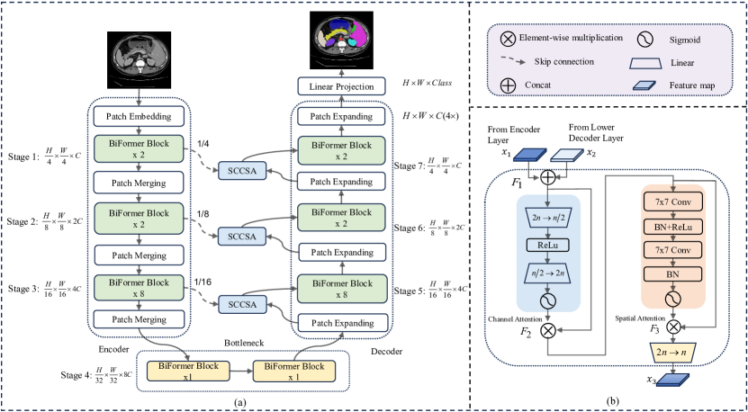
Figure 2: (a): The architecture of our BRAU-Net++, which is constructed based on BiFormer block. (b): The skip connection channel-spatial attention (SCCSA) module, which enhances the ability of cross-dimension interactions from both channel and spatial aspects and compensates the spatial information loss caused by down-sampling.

3.3 BiFormer Block

The core of the building block is bi-level routing attention (BRA). As illustrated in Fig. 3, the BiFormer block consists of a 3$\times$3 depth-wise convolution at the beginning, 2 LayerNorm (LN) layers, a BRA module, 3 residual connections and a 2-layer MLP with expansion ratio $e$ = 3. The 3$\times$3 depth-wise convolution can implicitly encode relative position information. The BiFormer block can be formulated as:

$${\hat{z}^{l-1}}=DW({z^{l-1}})+{z^{l-1}},$$ (6)

$${\hat{z}^{l}}=BRA(LN({\hat{z}^{l-1}}))+{\hat{z}^{l-1}},$$ (7)

$${z^{l}}=MLP(LN({\hat{z}^{l}}))+{\hat{z}^{l}},$$ (8)

where ${\hat{z}^{l-1}}$, ${\hat{z}^{l}}$ and ${z^{l}}$ represent the outputs of the depth-wise convolution, BRA module and MLP module of the ${l^{th}}$ block, respectively.

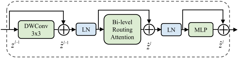
Figure 3: Details of a BiFormer block.

3.4 Encoder

The encoder is hierarchically constructed by using a three-stage pyramid structure. Specifically, a patch embedding layer consisting of two 3$\times$3 convolution layers, in stage 1, and a patch merging layer with a 3$\times$3 convolution layer, in stages 1–3, are used to reduce the input spatial resolution while increasing the number of channels. As illustrated in Fig. 2, the tokenized inputs with the resolution of $\frac{H}{4}\times\frac{W}{4}$ and C channels are fed into the two consecutive BiFormer blocks in stage 1 to perform representation learning. The tokenized inputs in stages 2–3 are also performed in a similar manner. The patch merging layer performs a 2$\times$ down-sampling to decrease the number of tokens by half, and increases feature dimension by 2$\times$.

3.5 Decoder

Similar to the encoder, the decoder is also built based on BiFormer block. Inspired by Swin-Unet [35], we also adopt the patch expanding layer to up-sample the extracted deep features in the decoder. The patch expanding layer is mainly used to reshape feature maps into a higher resolution feature map, i.e., increasing the resolution by 2$\times$, and decrease the feature dimension by half. The last patch expanding layer performs 4$\times$ up-sampling to output the feature map of the resolution $H\times W$, which is used to predict pixel-level segmentation.

3.6 Skip Connection Channel-Spatial Attention (SCCSA)

The combination of channel and spatial attention can enhance the model’s ability to capture a wider range of contextual features compared to using a single attention mechanism. Inspired by [39], we consider to applying a sequential channel-spatial attention mechanism to skip connection, and thus propose a skip connection channel-spatial attention, SCCSA for short. The SCCSA module can effectively compensate the loss of spatial information caused by down-sampling and enhance global dimension-interaction of multi-scale features for each layer of the decoder, and thus enabling the recovery of fine-grained details while generating output masks. As presented in Fig. 2(b), the SCCSA module includes a channel attention submodule and a spatial attention submodule. Specifically, we first derive ${F_{1}}\in{{\mathbb{R}}^{h\times w\times 2n}}$, via concatenating the output from both the encoder and the decoder. Then, the channel attention submodule magnifies cross-dimension channel-spatial dependencies using an encoder-decoder structure of multi-layer perceptron (MLP) with reduction ratio $e$ = 4. We use two 7$\times$7 convolution layers to focus on spatial information with the same reduction ratio $e$ from the channel attention submodule. Given the input feature map ${x_{1}},{x_{2}}\in{{\mathbb{R}}^{h\times w\times n}}$, the intermediate states ${F_{1}},{F_{2}},{F_{3}}$, and then the output ${x_{3}}$ is defined as:

$${F_{1}}=Concat({x_{1}},{x_{2}}),$$ (9)

$${F_{2}}=\sigma(FC({\mathop{\rm Re}\nolimits}Lu(FC({F_{1}})))\otimes{F_{1}},$$ (10)

$${F_{3}}=\sigma(Conv({\mathop{\rm Re}\nolimits}Lu(BN(Conv({F_{2}})))))\otimes{F_{2}},$$ (11)

$${x_{3}}=FC({F_{3}}).$$ (12)

Where ${F_{2}}$ and ${F_{3}}$ are the output of channel and spatial attention submodule, respectively; $\otimes$ and $\sigma$ denote element-wise multiplication and sigmoid activation function, respectively.

3.7 Loss Function

During training, for Synapse dataset, we employ a hybrid loss that combines both dice loss and cross-entropy loss to address the problems related to class imbalance. For ISIC-2018 and CVC-ClinicDB datasets, we employ the dice loss to optimize our model. The dice loss ($\cal L$_dice), cross-entropy loss ($\cal L$_ce), and the hybrid loss ($\cal L$) are defined as follows:

$${\mathcal{L}_{dice}}=1-\sum\limits_{k}^{K}{\frac{{2{\omega_{k}}\sum\nolimits_{i}^{N}{p(k,i)g(k,i)}}}{{\sum\nolimits_{i}^{N}{{p^{2}}(k,i)+\sum\nolimits_{i}^{N}{{g^{2}}(k,i)}}}}},$$ (13)

$$\mathcal{L}_{ce}= -\frac{1}{N}\sum_{i=1}^{N}G(k,i)\cdot\log(P(k,i))$$ (14)

$$+(1-G(k,i))\cdot\log(1-P(k,i)),$$

$$\mathcal{L}=\lambda{\mathcal{L}_{dice}}+(1-\lambda){\mathcal{L}_{ce}},$$ (15)

where $N$ is the number of pixels, $G(k,i)\in(0,1)$ and $P(k,i)\in(0,1)$ indicate the ground truth label and the produced probability for class $k$, respectively. $K$ is the number of class, and $\sum\nolimits_{k}{{\omega_{k}}}$ = 1 is weight sum of all class. $\lambda$ is a weighted factor that balances the impact of $\mathcal{L}_{dice}$ and $\mathcal{L}_{ce}$. In our study, The ${\omega_{k}}$ and $\lambda$ are empirically set as $\frac{1}{K}$ and 0.6, respectively. The training procedure of our BRAU-Net++ is summarized in Algorithm 1.

input : Images $S$ = $\{{x_{i}},i\in{{\mathbb{N}}}\}$, Masks $T$ = $\{{y_{i}^{t}},i\in{{\mathbb{N}}}\}$

output : Model parameters

1 for $i=0\to batch$ $size$ do

2       ${x}=Patch$ $Embedding({x_{i}})$

3       for $m=0\to num\_stage$ do

4             for $n=0\to num\_stage\_block$ do

5                   ${x}={x}+pos\_embed({x})$

6                   ${x}={x}+BRA({x})$

7                   ${x}={x}+MLP({x})$

8             end for

9            ${x_{m}}=Patch$ $Merging({x})$

10             ${temp_{m}}={x_{m}}$

11       end for

12      for $i=num\_stage-2\to-1$ do

13             ${x_{i}}=Patch$ $Expanding({x})$

14             ${x}=Concat({temp_{i}},{x_{2-i}})$

15             ${x}=SCCSA({x})$

16            

17            for $j=0\to num\_stage\_block$ do

18                   ${x}={x}+pos\_embed({x})$

19                   ${x}={x}+BRA({x})$

20                   ${x}={x}+MLP({x})$

21             end for

22            

23       end for

24      ${x}=Patch$ $Expanding$ 4x$({x})$

25       ${y_{i}^{out}}=Linear$ $Projection({x})$

26       Calculating the loss, $\cal L$ $\leftarrow$ $\lambda$ $\cdot$ $\cal L$_dice(${y_{i}^{out}}$, ${y_{i}^{t}}$) $+(1-\lambda)\cdot$ $\cal L$_ce(${y_{i}^{out}}$, ${y_{i}^{t}}$)

27       Gradient back propagation, update parameters

28 end for

Algorithm 1 The training procedure of BRAU-Net++

4 Experimental Settings

4.1 Datasets

We train and test the proposed BRAU-Net++ on three publicly available medical image segmentation datasets: Synapse multi-organ segmentation [56], ISIC-2018 Challenge [42], [43], and CVC-ClinicDB [44]. The details about data split are presented in Table 1. All the datasets are related to clinical diagnosis, making their segmentation results crucial for the treatment of patients, and consist of the images and their corresponding ground truth masks. The main reason for choosing diverse imaging modalities datasets is to evaluate the performance and robustness of the proposed method.

Table 1: Details of the medical segmentation datasets used in our experiments.

Dataset	Input Size	Total	Train	Valid	Test
Synapse	224$\times$224	3379	2212	1167	-
ISIC-2018	256$\times$256	2594	1868	467	259
CVC-ClinicDB	256$\times$256	612	490	61	61

4.1.1 Synapse Multi-Organ Segmentation Dataset

Automatic multi-organ segmentation on abdominal computed tomography (CT) can support clinical diagnosis, treatment planning, and treatment delivery workflows. The dataset used in experiments includes 30 abdominal CT scans from the MICCAI 2015 Multi-Atlas Abdomen Labeling Challenge, with 3,779 axial abdominal clinical CT images. Each CT volume involves 85–198 slices of 512$\times$512 pixels, with a voxel spatial resolution of ([0.54–0.54]$\times$[0.98–0.98]$\times$[2.5–5.0]) ${\operatorname{mm}^{3}}$. Following [1], [35], both training set and testing set consist of 18 (containing 2,212 axial slices) and 12 samples, respectively.

4.1.2 ISIC-2018 Challenge Dataset

The dataset in this work refers to the training set used for the lesion segmentation task in the ISIC-2018 Challenge, which contains 2,594 dermoscopic images with ground truth segmentation annotations. The fivefold cross-validation is performed to evaluate the performance of model, and select the best model to inference.

4.1.3 CVC-ClinicDB Dataset

The CVC-ClinicDB dataset is commonly used for polyp segmentation task. It is also the training dataset for the MICCAI 2015 Sub-Challenge on Automatic Polyp Detection Challenge. This dataset contains 612 images, which is randomly divided into 490 training images, 61 validation images, and 61 testing images.

4.2 Evaluation Metrics

To evaluate the performance of the proposed BRAU-Net++, the average Dice-Similarity Coefficient (DSC) and average Hausdorff Distance (HD) are considered as evaluation metrics to evaluate our method on 8 abdominal organs: aorta, gallbladder, spleen, left kidney, right kidney, liver, pancreas, spleen, and stomach, and only DSC is exclusively used on the evaluation of individual organ. Moreover, the mean Intersection over Union (mIoU), DSC, Accuracy, Precision, and Recall etc. are taken as evaluation metrics for the performance of models on both ISIC-2018 Challenge and CVC-ClinicDB datasets. Formally, the prediction can be separated into True Positive (TP), False Positive (FP), True Negative (TN), and False Negative (FN), and then DSC, IoU, Accuracy, Precision and Recall are calculated as:

$$\operatorname{DSC}=\frac{{2\times TP}}{{2\times TP+FP+FN}},$$ (16)

$$\operatorname{IoU}=\frac{{TP}}{{TP+FP+FN}},$$ (17)

$$\operatorname{Accuracy}=\frac{{TP+TN}}{{TP+TN+FP+FN}},$$ (18)

$$\operatorname{Precision}=\frac{{TP}}{{TP+FP}},$$ (19)

$$\operatorname{Recall}=\frac{{TP}}{{TP+FN}}.$$ (20)

HD can be described as:

$$\operatorname{HD}(Y,\hat{Y})=\max\{\mathop{\max}\limits_{y\in Y}\mathop{\min}\limits_{\hat{y}\in\hat{Y}}d(y,\hat{y}),\mathop{\max}\limits_{\hat{y}\in\hat{Y}}\mathop{\min}\limits_{y\in Y}d(y,\hat{y})\},$$ (21)

where $Y$ and $\hat{Y}$ are the ground truth mask and predicted segmentation map, respectively. $d(y,\hat{y})$ denotes the Euclidean distance between points $y$ and $\hat{y}$.

4.3 Implementation Details

We train our BRAU-Net++ model and its various ablation variants on an NVIDIA 3090 graphics card with 24GB memory. We implement our approach using Python 3.10 and PyTorch 2.0 [57]. During training, we initialize and fine-tune the model on the above-mentioned three datasets, with the weights from BiFormer [24] pretrained on ImageNet-1K [58], and considering space, also train the proposed model from scratch only on Synapse multi-organ segmentation dataset. On these resulting models, we conduct a serial of ablation studies to analyze the contribution of each component.

With respect to the Synapse multi-organ segmentation dataset, we resize all the images to the resolution of 224$\times$224, and train the model using stochastic gradient descent for 400 epochs, with a batch size of 24, learning rate of 0.05, momentum of 0.9, and weight decay of 1e-4. With regard to both ISIC-2018 Challenge and CVC-ClinicDB datasets, we resize all the images to resolution 256$\times$256, and train all the models using Adam [59] optimizer for 200 epochs, with a batch size of 16. We apply CosineAnnealingLR schedule with an initial learning rate of 5e-4. The data augmentations such as horizontal flip, vertical flip, rotation, and cutout with the probability of 0.25 are used to enhance the data diversity.

Other hyper-parameters are also empirically set. For example, the region partition factor $S$ is set as 7 and 8 according to the resolution of 224$\times$224 and 256$\times$256, respectively. The number of top-$k$ from stage 1 to stage 7 is set to 2, 4, 8, $S^{2}$, 8, 4, and 2, respectively, in which $S^{2}$ means using full attention.

5 Experimental Results

In this section, we elaborate on the comparisons of the proposed BRAU-Net++ with other state-of-the-art (SOTA) methods including CNN-based, transformer-based, and hybrid approaches of both on the Synapse multi-organ segmentation, ISIC-2018 Challenge, and CVC-ClinicDB datasets. Also, we take Synapse multi-organ segmentation dataset as an exemplar, on which we conduct extensive ablation studies to analyze the effect of each component of our approach.

5.1 Comparison on Synapse Multi-Organ Segmentation

As mentioned above, the automatic multi-organ abdominal CT segmentation plays an essential role in improving the efficiency of clinical workflows including disease diagnosis, prognosis analysis, and treatment planning. So, we select this dataset to evaluate the performance of various methods. The comparison of our proposal with previous SOTA methods in terms of DSC and HD on Synapse multi-organ abdominal CT segmentation dataset is shown in Table 2 with the best results in bold. The results of [32], [60], [33], [34] are reproduced under our experimental settings according to the publicly released codes, while other results are directly from the respective published paper. Our BRAU-Net++ outperforms CNN-based methods and our baseline: BRAU-Net on both evaluation metrics by a large margin, which demonstrates that deeper hybrid CNN-Transformer model may be capable of modeling global relationships and local representations. Compared to both prevailing transformer-based methods: TransUNet and Swin-Unet, our BRAU-Net++ has a significant increase of 4.49% and 3.34% on DSC, and a remarkable decrease of 12.62mm and 2.48mm on HD, respectively. This indicates using bi-level routing attention as core building block to design u-shaped encoder-decoder structure may be helpful for effectively learning global semantic information. More concretely, the BRAU-Net++ steadily beats other methods w.r.t. the segmentation of most organs, particularly for left kidney and liver segmentation. It can be seen from Table 2 that the DSC value obtained by our method is highest, reaching up to 82.47%, which shows that the segmentation map predicted by our method has a higher overlap with the ground-truth mask than other methods. One can also observe that we achieve a relatively low value (19.07mm) on HD compared to HiFormer and MISSFormer, which yields the best (14.7mm) and second-best (18.20mm) results, respectively. BRAU-Net++ just raises by 0.87mm on HD than MISSFormer, but has visibly increase of 4.37mm than HiFormer, which denotes that the ability of our methods to learn the edge information of target may be inferior to that of HiFormer. As a whole, Table 2 shows that except for HiFormer and MISSFormer, the proposed BRAU-Net++ has significant improvements over prior works, e.g., performance gains range from 0.51% to 12.2% on DSC, and from 1.59mm to 20.63mm on HD, respectively. Thus, we believe that our approach has still a potential to obtain a relatively better segmentation result.

Also, one can see from Table 2 that the numbers of parameters of BRAU-Net++ has about learnable parameters of 50.76M, in which SCCSA module yield about 19.36M parameters. But the BRAU-Net++ with SCCSA module slightly improves the performance on DSC than without SCCSA module. There is also a similar observation on HD. The efficiency in terms of the number of parameters will be discussed in the following sections.

Some qualitative results of different methods on the Synapse dataset are given in Fig. 4. It can be seen from Fig. 4 that our method generates a smooth segmentation map for gallbladder, left kidney and pancreas, which demonstrate that the bi-level routing attention may excel at capturing the features of small targets, and the BRAU-Net++ can better learn both global and long-range semantic information, thus yielding better segmentation results.

Table 2: The quantitative results on Params, DSC, and HD of different methods on the Synapse multi-organ CT dataset. Only DSC is exclusively used for the evaluation of individual organ. The symbol $\uparrow$ indicates the larger the better. The symbol $\downarrow$ indicates the smaller the better. The best result is in Blod, and the second best is underlined.

Methods	Params (M)	DSC (%) $\uparrow$	HD (mm) $\downarrow$	Aorta	Gallbladder	Kidney(L)	Kidney(R)	Liver	Pancreas	Spleen	Stomach
U-Net [8]	14.80	76.85	39.70	89.07	69.72	77.77	68.60	93.43	53.98	86.67	75.58
Attention U-Net [11]	34.88	77.77	36.02	89.55	68.88	77.98	71.11	93.57	58.04	87.30	75.75
BRAU-Net [38]	67.31	70.27	32.91	78.51	61.69	72.94	67.90	93.14	40.88	84.42	62.68
TransUNet [1]	105.28	77.48	31.69	87.23	63.13	81.87	77.02	94.08	55.86	85.08	75.62
Swin-Unet [35]	27.17	79.13	21.55	85.47	66.53	83.28	79.61	94.29	56.58	90.66	76.60
HiFormer [32]	25.51	80.39	14.70	86.21	65.69	85.23	79.77	94.61	59.52	90.99	81.08
PVT-CASCADE [60]	35.28	81.06	20.23	83.01	70.59	82.23	80.37	94.08	64.43	90.10	83.69
Focal-UNet [33]	32.40	80.81	20.66	85.74	71.37	85.23	82.99	94.38	59.34	88.49	78.94
MISSFormer [34]	42.46	81.96	18.20	86.99	68.65	85.21	82.00	94.41	65.67	91.92	80.81
BRAU-Net++(w/o SCCSA)	31.40	81.65	19.46	86.80	69.73	86.53	82.24	94.69	64.23	89.69	79.26
BRAU-Net++	50.76	82.47	19.07	87.95	69.10	87.13	81.53	94.71	65.17	91.89	82.26

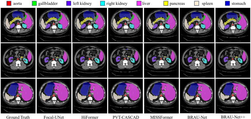
Figure 4: The segmentation results of different methods on the Synapse multi-organ CT dataset. Our BRAU-Net++ shows a relatively better visualization than other methods.

5.2 Comparison on ISIC-2018 Challenge

It is well known that melanoma is a commonly occurring cancer, which if detected and treated in time, up to 99th-percentile of lives can be saved. So, an automated diagnostic tool for skin lesions is extremely helpful for accurate melanoma detection. We perform fivefold cross-validation on the ISIC-2018 Challenge dataset to evaluate the performance of our method to avoid overfitting. We reproduce the results of all methods based on the publicly released codes. The quantitative and qualitative results are presented in Table 3 and in Fig. 5 (left). Our method achieves mIoU of 84.01, DSC of 90.10, Accuracy of 95.61, Precision of 91.18, and Recall of 92.24, in which our method achieves the best performance in terms of mIoU, DSC, and Accuracy, and second-best result in terms of Precision and Recall. One can observe that the proposed BRAU-Net++ obtains improvements of 1.84% and 1.2% on mIoU over recently published DCSAU-Net and BRAU-Net, respectively. Also, our method achieves a recall of 0.9224, which is more favorable in clinic applications. From the above analysis and Fig. 5 (left), it can be evidently seen that BRAU-Net++ achieves better boundary segmentation predictions against other methods on ISIC-2018 Challenge dataset. The contours of the segmented masks by BRAU-Net++ are closer to ground truth.

Table 3: The qualitative results on the ISIC-2018 Challenge.

Methods	mIoU $\uparrow$	DSC $\uparrow$	Accuracy $\uparrow$	Precision $\uparrow$	Recall $\uparrow$
U-Net [8]	80.21	87.45	95.21	88.32	90.60
Attention U-Net [11]	80.80	86.31	95.44	91.52	89.01
MedT [36]	81.43	86.92	95.10	90.56	89.93
TransUNet [1]	77.05	84.97	94.56	84.77	89.85
Swin-Unet [35]	81.87	87.43	95.44	90.97	91.28
BRAU-Net[38]	82.81	89.32	95.10	90.27	92.25
DCSAU-Net[46]	82.17	88.74	94.75	90.93	90.98
BRAU-Net++	84.01	90.10	95.61	91.18	92.24

Table 4: The qualitative results on the CVC-ClinicDB.

Methods	mIoU $\uparrow$	DSC $\uparrow$	Accuracy $\uparrow$	Precision $\uparrow$	Recall $\uparrow$
U-Net [8]	80.91	87.22	98.45	88.24	89.35
Attention U-Net [11]	83.54	89.57	98.64	90.47	90.10
MedT [36]	81.47	86.97	98.44	89.35	90.04
TransUNet [1]	79.95	86.70	98.25	87.63	87.34
Swin-Unet [35]	84.85	88.21	98.72	90.52	91.13
BRAU-Net [38]	77.45	83.64	97.96	84.56	84.20
DCSAU-Net[46]	86.18	91.67	99.01	91.72	92.03
BRAU-Net++	88.17	92.94	98.83	93.84	93.06

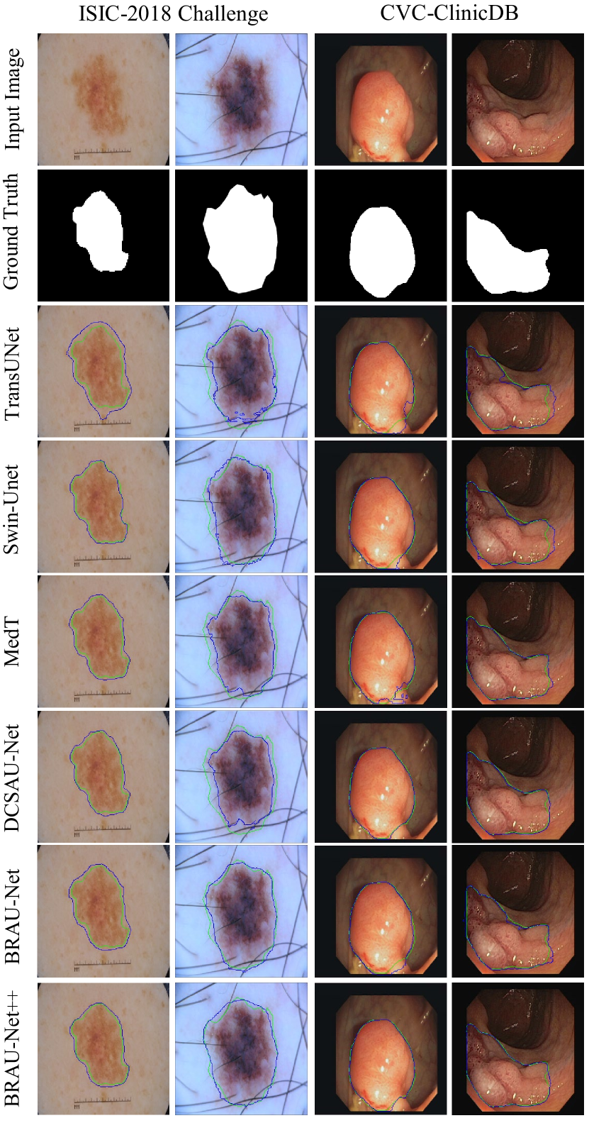
Figure 5: The visual segmentation results of different methods on the ISIC-2018 Challenge and CVC-ClinicDB datasets. Ground truth boundaries are shown in green, and predicted boundaries are shown in blue.

5.3 Comparison on CVC-ClinicDB

Before the polyp has a potential to change into colorectal cancer, early detection can improve the survival rate. This is of great significance to clinical practice. Therefore, we have selected this dataset in our experiment. The quantitative results presented in Table 4. Our proposed method achieves best results on mIoU (88.17), DSC (92.94), Precision (93.84), and Recall (93.06), surpassing the second-best by 1.99%, 1.27%, 2.12%, and 1.03%, respectively. The qualitative results are shown in Fig. 5 (right). One can see that the polyp masks generated by our approach closely match the boundaries and shape of the ground truth.

5.4 Ablation Study

In this section, we conduct an extensive ablation study on the above mentioned three datasets, so as to thoroughly evaluate the effectiveness of each component involved in BRAU-Net++. Specifically, we ablate the impacts of SCCSA module, the number of skip connections and top-$k$, input size and partition factor $S$, as well as model scales and pre-trained weights.

5.4.1 Effectiveness of SCCSA Module

The SCCSA module is an essential part of the proposed BRAU-Net++. It uses channel-spatial attention to enhance the cross-dimension interactions on both channel and spatial aspects and help to generate a more accurate segmentation mask. Table 2 shows the results of BRAU-Net++ without and with SCCSA module on the Synapse. Compare with BRAU-Net++ without SCCSA, BRAU-Net++ achieves a better segmentation performance, increasing by 0.91% on DSC and decreasing by 0.39mm on HD evaluation metric, respectively. Such a slight improvement comes at a cost: it brings a huge number of parameters into this model. One main reason may be that the combination of multi-scale CNN features with global semantic features learned by the hierarchical transformer structure cannot significantly benefit the segmentation task. With respective to the exactly reasons, we intend to leave them as future work to further explore and analyze. The segmentation results on ISIC-2018 Challenge and CVC-ClinicDB datasets are presented in Table 5. One can see that adding SCCSA module into BRAU-Net++ model can achieve best results under almost all evaluation metrics. For example, SCCSA can help improve by 0.6% on ISIC-2018 Challenge and by 0.9% on CVC-ClinicDB w.r.t. mIoU metric, respectively. In addition, the number of parameters, floating point operations (FLOPs) and frames per second (FPS) are calculated to further investigate the effectiveness of this module. We can observe that SCCSA do not significantly harm FPS on the two datasets, particularly for CVC-ClinicDB.

Table 5: Ablation study on the impact of SCCSA module on both ISIC-2018 Challenge and CVC-ClinicDB datasets.

Dataset	Methods	Params (M)	FLOPs (G)	FPS	mIoU $\uparrow$	DSC $\uparrow$	Accuracy $\uparrow$	Precision $\uparrow$	Recall $\uparrow$
ISIC-2018 Challenge	BRAU-Net++ (w/o SCCSA)	31.40	11.12	17.26	83.47	89.75	95.54	91.01	91.97
	BRAU-Net++	50.76	22.45	29.84	84.01	90.10	95.61	91.18	92.24
CVC-ClinicDB	BRAU-Net++ (w/o SCCSA)	31.40	11.06	15.95	87.37	92.64	98.85	93.99	92.01
	BRAU-Net++	50.76	22.39	15.56	88.17	92.94	98.83	93.84	93.06

5.4.2 Effectiveness of the Number of Skip Connections

It has been witnessed that skip connections of u-shaped network can help improve finer segmentation details by recovering low-level spatial information. This ablation mainly aims to explore the impact of the different numbers of skip-connections for the performance boosting of our BRAU-Net++. This experiment is conducted on Synapse dataset. The skip connections are added at the places of 1/4, 1/8, and 1/16 resolution scales, and the number of skip connections can be changed to be 0, 1, 2, and 3 through the combination of connections at different places, in which “0” indicates that no skip connection is added. Other added connections and their corresponding segmentation performance on average DSC and HD metrics are presented in Table 6. We can observe that with the increase of the number of skip connections, the segmentation performance gradually increases, and best average DSC and HD are achieved by adding the skip connections at all places of 1/4, 1/8, and 1/16 resolution scales. Thus, we adopt this configuration for our BRAU-Net++ to enhance the ability to learn precise low-level details. This may be main reason that BRAU-Net++ can capture the features of small targets.

Table 6: Ablation study on the number of skip connections.

# Skip Connection	Connection Place				DSC $\uparrow$	HD $\downarrow$
	no skip	1/4	1/8	1/16
0	$\checkmark$				76.40	28.36
1		$\checkmark$			78.56	26.14
2		$\checkmark$	$\checkmark$		81.16	22.67
3		$\checkmark$	$\checkmark$	$\checkmark$	82.47	19.07

5.4.3 Effectiveness of Input Resolution and Partition Factor S

The main goal of conducting this ablation is to test the impact of input resolution on model performance. We perform three groups of experiments on 128$\times$128, 224$\times$224, and 256$\times$256 resolution scales on Synapse dataset, and report the results in Table 7. Following [24], partition factor $S$ is selected as a divisor of the size of feature maps in every stage to avoid padding, and the images with different input resolutions should adopt different partition factors $S$. Thus, we set the corresponding partition factor of the above three resolutions as $S$ = 4, $S$ = 7, and $S$ = 8. It can be seen that keeping patch size same (e.g., 32) and gradually increasing the resolution scales, i.e., increasing the sequence length of the tokens can lead to the consistent improvement of model performance. It accords with the common sense that the larger resolution images contain more semantic information, and thus boosting the performance. However, this is at the expense of much larger computational cost. Therefore, considering the computation cost, and to fair the comparison with other methods, all the experiments are performed based on a default resolution of 224$\times$224 as the input.

Table 7: Ablation study on the input resolution and partition factor $S$. The symbol ${\dagger}$ denotes the original resolution.

	Image Size				factor $S$			DSC $\uparrow$		HD $\downarrow$
	128$\times$128				4			77.99		25.29
	224$\times$224†				7			82.47		19.07
	256$\times$256				8			82.61		18.56

5.4.4 Effectiveness of the Number of Top-k.

Similar to [24], as the size of the routed region gradually reduces at the following stage, we accordingly increase $k$ to maintain a reasonable number of tokens to attention. The results of ablation on the number of top-$k$ on Synapse dataset is showed in Table 8, where the number of top-$k$ and tokens to attend in each stage of the network are listed. One can see that boosting the number of tokens in near top stages of encoder can seemingly improve the segmentation performance. That may be because the near top blocks of network can capture the low-level information e.g., edge or texture, which is essential for the segmentation task. Also, blindly increasing the number of tokens to attention may hurt the performance, which shows that explicit sparsity constraint can serve as a regularization to improve the generalization ability of model. This insight is similar to [24].

Table 8: Ablation study on the number of the top-$k$.

# top-$k$	# tokens to attend	DSC$\uparrow$	HD$\downarrow$
1,4,16,49,16,4,1	64,64,64,49,64,64,64	81.83	23.92
2,8,32,49,32,8,2	128,128,128,49,128,128,128	81.74	23.21
1,2,4,49,4,2,1	64,32,16,49,16,32,64	82.03	21.54
2,4,8,49,8,4,2	128,64,32,49,32,64,128	82.47	19.07
4,8,16,49,16,8,4	256,128,64,49,64,128,256	82.08	20.09

5.4.5 Effectiveness of Model Scale and Pre-trained Weights

Similar to [1], [35], we give the effect of network deepening. Also, as we all known, the performance of transformer-based model is severely affected by model pre-training. Thus, we consider to providing four ablation studies on two different model scales of BRAU-Net++ from the model trained from scratch and pre-trained aspects, respectively. The two different model scales of BRAU-Net++ are called the tiny and base models, respectively. Their configurations and results on Synapse dataset are listed in Table 9. One can see that the base model yields a more favorable result. Particularly on the HD evaluation metric, the result of the base model improves by 14.77mm compared to the tiny model. This suggests that the base model can achieve better edge predictions. Hence, we adopt the base model to perform medical image segmentation. Considering the computation performance, we adopt the “base” model for all the experiments.

Table 9: Ablation study on the model scale and pre-trained weights.

Model Scale		Channels	Params (M)	DSC$\uparrow$		HD$\downarrow$
tiny w/o pre-t		64	22.64	76.36		34.04
tiny		64	22.64	79.39		33.84
base w/o pre-t		96	50.76	78.48		23.84
base		96	50.76	82.47		19.07

6 Discussion

In this work, we show that the dynamic and query-aware sparse attention is effective on both reducing computational complexity and improving model performance. To further illustrate how the sparse attention works on medical image segmentation task, following [24], we visualize routed regions and attention response w.r.t. query tokens. We adopt routing indices and attention scores, which are extracted from the final block of the $3^{rd}$ stage in the encoder, for this visualization. That is, these values are obtained from the feature map of $\frac{H}{{16}}\times\frac{W}{{16}}$ resolution, while the visualizations are presented in the images of original resolution. The results on Synapse multi-organ segmentation, ISIC-2018 Challenge, and CVC-ClinicDB datasets are shown in Fig. 6. One can clearly see that the type of sparse attention can effectively find semantically most related regions, which indicates the dynamic sparse attention computation mechanism is effective for the calculation and selection of sparse patterns of medical images. However, exploring other efficient sparse pattern computation methods are still necessary, and also the focus of our future work.

We perform a series of ablation studies to evaluate the contribution of each related component of BRAU-Net++, in which we propose SCCSA module to enhance the cross-dimension interactions of these features from stage $i$ in the encoder and from stage $7-i$ in the decoder on both channel and spatial aspects. The experimental results are encouraging under almost all evaluation metrics. However, one can see from Table 2 that such a slight improvement comes at a cost of bringing a huge number of parameters. This is a shortcoming of our work. We believe main reason may be that the combination of multi-scale CNN features and global semantic features learned by the hierarchical transformer structure cannot significantly benefit the segmentation task. In future work, we will focus on how to effectively address this problem.

Three diverse imaging modalities datasets: Synapse multi-organ segmentation, ISIC-2018 Challenge, and CVC-ClinicDB, are deliberately chosen as benchmarks. The main reason of this choice is to evaluate the performance and robustness of the proposed method. Extensive experiments reveal the generality of our approach for multi-modal medical image segmentation task.

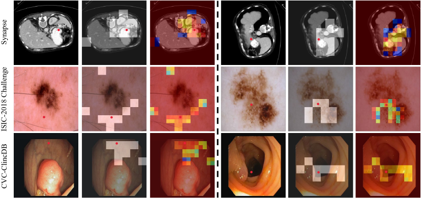
Figure 6: Similar to [24], visualization of attention maps on three datasets. For each dataset, we visualize a query position on the input image (left), corresponding routed regions (middle), and a final attention heatmap (right).

7 Conclusion

In this paper, we propose a well-designed u-shaped hybrid CNN-Transformer architecture, BRAU-Net++, which exploits dynamic sparse attention instead of full attention or static handcrafted sparse attention, and can effectively learn local-global semantic information while reducing computational complexity. Furthermore, we propose a novel module: skip connection channel-spatial attention (SCCSA) to integrate multi-scale features, so as to compensate the loss of spatial information and enhance the cross-dimension interactions. Experimental results show that our method can achieve SOTA performance under almost all evaluation metrics on Synapse multi-organ segmentation, ISIC-2018 Challenge, and CVC-ClinicDB datasets, and particularly excels at capturing the features of small targets. For future work, we will focus on how to design more sophisticate and general architecture for multi-modal medical image segmentation task.

References

References

- [1] J. Chen, Y. Lu, Q. Yu, X. Luo, E. Adeli, Y. Wang, L. Lu, A. L. Yuille, and Y. Zhou, “TransUNet: Transformers make strong Encoders for medical image segmentation,” arXiv:2102.04306, 2021.
- [2] A. Srivastava et al., “MSRF-Net: A multi-scale residual fusion network for biomedical image segmentation,” IEEE J. Biomed. Health. Inf. , vol. 26, no. 5, pp. 2252–2263, May 2022.
- [3] R. Azad, Y. Jia, E. K. Aghdam, J. Cohen-Adad, and D. Merhof, “Enhancing medical image segmentation with TransCeption: A multi-scale feature fusion approach,” arXiv:2102.04306, 2023.
- [4] J. Li, M. Erdt, F. Janoos, T. Chang, and Jan Egger, “Medical image segmentation in oral-maxillofacial surgery,” in Computer-Aided Oral and Maxillofacial Surgery, J. Egger and X. Chen, Ed. Academic Press, 2021, pp. 1–27.
- [5] A. S. Ashour, Y. Guo, and W. S. Mohamed, “Image-guided thermal ablation therapy,” in Thermal Ablation Therapy, A. S. Ashour, Y. Guo, and W. S. Mohamed, Ed. Academic Press, 2021, pp. 411–440.
- [6] Z. Zhou et al., “UNet++: A nested U-Net architecture for medical image segmentation,” in Deep Learn. Med. Imag. Anal. Multimodal Learn. Clin. Decis. Support, 2018, pp. 3–11.
- [7] X. Chen et al., “Learning Active Contour Models for Medical Image Segmentation,” in Proc. IEEE Conf. Comput. Vis. Pattern Recog., Long Beach, CA, USA, 2019, pp. 11624–11632.
- [8] O. Ronneberger, P. Fischer, and T. Brox, “U-Net: Convolutional networks for biomedical image segmentation,” in Proc. Int. Conf. Med. Imag. Comput. Comput.-Assist. Interv., 2015, pp. 234–241.
- [9] J. Long, E. Shelhamer, and T. Darrell, “Fully convolutional networks for semantic segmentation,” in Proc. IEEE Conf. Comput. Vis. Pattern Recognit., Boston, MA, USA, 2015, pp. 3431–3440.
- [10] H. Huang et al., “UNet 3+: A full-scale connected unet for medical image segmentation,” in Proc. IEEE Int. Conf. Acoust. Speech Signal Process., Barcelona, Spain, 2020, pp. 1055–1059.
- [11] O. Oktay et al., “Attention U-Net: Learning where to look for the pancreas,” arXiv:1804.03999, 2018.
- [12] Ö. Çiçek et al., “3D U-Net: Learning dense volumetric segmentation from sparse annotation,” in Proc. Int. Conf. Med. Imag. Comput. Comput.-Assist. Interv., 2016, pp. 424–432.
- [13] F. Milletari, N. Navab, and S. -A. Ahmadi, “V-Net: Fully convolutional neural networks for volumetric medical image segmentation,” in Proc. IEEE 4th Int. Conf. 3D Vis., Stanford, CA, USA, 2016, pp. 565–571.
- [14] L. -C. Chen, G. Papandreou, I. Kokkinos, K. Murphy, and A. L. Yuille, “DeepLab: Semantic image segmentation with deep convolutional nets, atrous convolution, and fully connected CRFs,” EEE Trans. Pattern Anal. Mach. Intell., vol. 40, no. 4, pp. 834–848, Apr. 2018.
- [15] Z. Gu et al., “Context encoder network for 2D medical image segmentation,” IEEE Trans. Med. Imag., vol. 38, no. 10, pp. 2281–2292, Oct. 2019.
- [16] X. Wang, R. Girshick, A. Gupta, and K. He, “Non-local neural networks,” in Proc. IEEE Conf. Comput. Vis. Pattern Recognit., Salt Lake City, UT, USA, 2018, pp. 7794–7803.
- [17] J. Schlemper et al., “Attention gated networks: Learning to leverage salient regions in medical images,” Med. Image Anal., vol. 53, pp. 197–207, Apr. 2019.
- [18] H. Zhao, J. Shi, X. Qi, X. Wang, and J. Jia, “Pyramid scene parsing network,” in Proc. IEEE Conf. Comput. Vis. Pattern Recognit., Honolulu, HI, USA, 2017, pp. 6230–6239.
- [19] A. Vaswani, N. Shazeer, N. Parmar, J. Uszkoreit, L. Jones, A. N. Gomez, L. Kaiser, and I. Polosukhin, “Attention is all you need,” in Proc. Adv. Neural Inf. Process. Syst., 2017, pp.5998–6008.
- [20] N. Carion, F. Massa, G. Synnaeve, N. Usunier, A. Kirillov, and S. Zagoruyko, “End-to-end object detection with transformers,” in Proc. Eur. Conf. Comput. Vis., 2020, pp. 213–229.
- [21] A. Dosovitskiy et al., “An image is worth 16x16 words: Transformers for image recognition at scale,” in Proc. Int. Conf. Learn. Representations, 2021.
- [22] H. Touvron et al., “Training data-efficient image transformers & distillation through attention,” Proc. Mach. Learn. Res., vol. 139, pp. 10347–10357, Jul. 2021.
- [23] Z. Liu et al., “Swin Transformer: Hierarchical vision transformer using shifted windows,” in Proc. IEEE Int. Conf. Comput. Vis., Montreal, QC, Canada, 2021, pp. 9992–10002.
- [24] L. Zhu, X. Wang, Z. Ke, W. Zhang, and R. Lau, “Biformer: Vision transformer with bi-level routing attention,” in Proc. IEEE Conf. Comput. Vis. Pattern Recognit., Vancouver, BC, Canada, 2023, pp. 10323–10333.
- [25] S. Tang, J. Zhang, S, Zhu, and P. Tan, “Quadtree attention for vision transformers,” in Proc. Int. Conf. Learn. Representations, 2023.
- [26] Z. Tu, H. Talebi, H. Zhang, F. Yang, P. Milanfar, A. Bovik, and Y. Li, “MaxViT: Multi-axis vision transformer,” in Proc. Eur. Conf. Comput. Vis., 2022, pp. 459–479.
- [27] W. Wang, L. Yao, L. Chen, B. Lin, D. Cai, X. He, and W. Liu, “CrossFormer: A versatile vision transformer hinging on cross-scale attention,” in Proc. Int. Conf. Learn. Representations, 2022.
- [28] H. Wang, Y. Zhu, B. Green, H. Adam, A. Yuille, and L. Chen, “Axial-DeepLab: Stand-alone axial-attention for panoptic segmentation,” in Proc. Eur. Conf. Comput. Vis., 2020, pp. 108–126.
- [29] H. -Y. Zhou, J. Guo, Y. Zhang, X. Han, L. Yu, L. Wang, and Y. Yu, “nnFormer: Volumetric medical image segmentation via a 3D transformer,” IEEE Trans. Image Process., vol. 32, pp. 4036–4045, 2023.
- [30] Y. Gao, M. Zhou, and D. N. Metaxas, “UTNet: A hybrid transformer architecture for medical image segmentation,” in Proc. Int. Conf. Med. Imag. Comput. Comput.-Assist. Interv., 2021, pp. 61–71.
- [31] X. Dong et al., “CSWin Transformer: A general vision transformer backbone with cross-shaped windows,” in Proc. IEEE Conf. Comput. Vis. Pattern Recognit., New Orleans, LA, USA, 2022, pp. 12114–12124.
- [32] M. Heidari et al., “HiFormer: Hierarchical multi-scale representations using transformers for medical image segmentation,” in Proc. IEEE Winter Conf. Appl. Comput. Vis., Waikoloa, HI, USA, 2023, pp. 6191–6201.
- [33] M. Naderi, M. Givkashi, F. Piri, N. Karimi, and S. Samavi, “Focal-UNet: UNet-like focal modulation for medical image segmentation,” arXiv:2212.09263, 2022.
- [34] X. Huang, Z. Deng, D. Li, and X. Yuan, “MISSFormer: An effective medical image segmentation transformer,” arXiv:2109.07162, 2021.
- [35] H. Cao, Y. Wang, J. Chen, D. Jiang, X. Zhang, Q.Tian, and M. Wang, “Swin-Unet: Unet-like pure transformer for medical image segmentation,” in Proc. Eur. Conf. Comput. Vis., 2022, pp. 205–218.
- [36] J. M. J. Valanarasu et al., “Medical Transformer: Gated axial-attention for medical image segmentation,” in Proc. Int. Conf. Med. Imag. Comput. Comput.-Assist. Interv., 2021, pp. 61–71.
- [37] R. Child, S. Gray, A. Radford, I. Sutskever, “Generating long sequences with sparse transformers,” arXiv:1904.10509, 2019.
- [38] P. Cai, L. Jiang, Y. Li, and L. Lan, “Pubic symphysis-fetal head segmentation using pure transformer with bi-level routing attention,” arXiv:2310.00289, 2023.
- [39] Y. Liu et al., “Global Attention Mechanism: Retain information to enhance channel-spatial interactions,” arXiv:2112.05561, 2021.
- [40] X. Chu et al., “Twins: Revisiting the design of spatial attention in vision transformers,” in Proc. Adv. Neural Inf. Process. Syst., 2021, pp. 9355–9366.
- [41] K. Li et al., “Uniformer: Unifying convolution and self-attention for visual recognition” IEEE Trans. Pattern Anal. Mach. Intell., vol. 45, no. 10, pp. 12581–12600, Oct. 2023.
- [42] N. C. F. Codella et al., “Skin lesion analysis toward melanoma detection: A challenge at the 2017 International symposium on biomedical imaging (ISBI), hosted by the international skin imaging collaboration (ISIC),” in IEEE 15th Int. Symp. Biomed. Imaging, Washington, DC, USA, 2018, pp.168–172.
- [43] P. Tschandl, C. Rosendahl, and H. Kittler1, “Data Descriptor: The HAM10000 dataset, a large collection of multi-source dermatoscopic images of common pigmented skin lesions,” Sci. Data, 2018.
- [44] J. Bernal et al., “WM-DOVA maps for accurate polyp highlighting in colonoscopy: Validation vs. saliency maps from physicians,” Comput. Med. Imaging Graph., vol. 43, pp. 99–111, 2015.
- [45] B. Chen, Y. Liu, Z. Zhang, G. Lu, and A. W. K. Kong, “TransAttUnet: Multi-level attention-guided u-net with transformer for medical image segmentation,” IEEE Trans. Emerg. Topics Comput. Intell., 2023.
- [46] Q. Xu, Z. Ma, N. He, and W. Duan, “DCSAU-Net: A deeper and more compact split-attention U-Net for medical image segmentation,” Comput. Biol. Med., vol. 154, pp. 106626, 2023.
- [47] N. Siddique, S. Paheding, C. P. Elkin, and V. Devabhaktuni, “U-Net and its variants for medical image segmentation: A review of theory and applications,” IEEE Access, vol. 9, pp. 82031–82057, 2021.
- [48] R. Azad et al., “Medical image segmentation review: The success of U-Net,” arXiv:2211.14830, 2022.
- [49] A. Hatamizadeh et al., “UNETR: Transformers for 3D medical image segmentation,” in Proc. IEEE Winter Conf. Appl. Comput. Vis., Waikoloa, HI, USA, 2022, pp. 1748–1758.
- [50] A. Hatamizadeh, V. Nath, Y. Tang, D. Yang, H. R. Roth, and D. Xu, “Swin UNETR: Swin transformers for semantic segmentation of brain tumors in MRI images,” in Proc. Int. Conf. Med. Imag. Comput. Comput.-Assist. Interv. Brainlesion Workshop, 2021, pp. 272–284.
- [51] Y. Rao, W. Zhao, B. Liu, J. Lu, J. Zhou, and C. Hsieh, “DynamicViT: Efficient vision transformers with dynamic token sparsification,” in Proc. Adv. Neural Inf. Process. Syst., 2021, pp. 13937–13949.
- [52] J. Hu, L. Shen, and G. Sun, “Squeeze-and-excitation networks,” in Proc. IEEE Conf. Comput. Vis. Pattern Recognit., Salt Lake City, UT, USA, 2018, pp. 7132–7141.
- [53] M. Jaderberg, K. Simonyan, A, Zisserman, and K. Kavukcuoglu, “Spatial transformer networks,” in Proc. Adv. Neural Inf. Process. Syst., 2015.
- [54] S. Woo et al., “CBAM: Convolutional block attention module,” in Proc. Eur. Conf. Comput. Vis., 2018, pp. 3–19.
- [55] Z. Xia, X. Pan, S. Song, L. E. Li, and G. Huang. “Vision transformer with deformable attention,” in Proc. IEEE Conf. Comput. Vis. Pattern Recognit., New Orleans, LA, USA, 2022, pp. 4784–4793
- [56] B. Landman et al., “Synapse Multi-Organ Abdominal CT Segmentation Dataset,” Multi-Atlas Labeling Beyond the Cranial Vault–Workshop and Challenge, [Online]. Available: https://www.synapse.org/#!Synapse:syn3193805/wiki/217789.
- [57] A. Paszke et al., “Automatic differentiation in PyTorch,” in Proc. Adv. Neural Inf. Process. Syst., 2017, pp. 1–4.
- [58] J. Deng, W. Dong, R. Socher, L.-J. Li; K. Li, and Li Fei-Fei, “ Imagenet: A large-scale hierarchical image database,” in Proc. IEEE Conf. Comput. Vis. Pattern Recognit., Miami, FL, USA, 2009, pp. 248–255.
- [59] D. Kingma, and J. Ba, “Adam: A method for stochastic optimization,” in Proc. Int. Conf. Learn. Representations, 2015.
- [60] M. M. Rahman, and R. Marculescu, “Medical image segmentation via cascaded attention decoding,” in Proc. IEEE Winter Conf. Appl. Comput. Vis., Waikoloa, HI, USA, 2023, pp. 6211–6220.