Update on flavor diagonal nucleon charges from clover fermions

Abstract

We present a summary of the full calculation of the axial, scalar and tensor flavor diagonal charges of the nucleon carried out using Wilson-clover fermions on eight ensembles generated using 2+1+1-flavors of highly improved staggered quarks (HISQ) by the MILC collaboration. We also give results for the $3\times 3$ matrix of renormalization factors between the RI-sMOM and $\overline{\rm MS}$ scheme for the 2+1 flavor theory that include flavor mixing. Preliminary results for $g_{A,S,T}^{u,d,s}$ are presented in the $\overline{\rm MS}$ scheme at scale 2 GeV.

1 Introduction

We present lattice QCD results for flavor diagonal nucleon charges $g_{A,S,T}^{u,d,s}$ extracted from the matrix elements, within ground state nucleons, of axial, scalar, and tensor quark bilinear operators, ${\overline{q}}\Gamma q$ with the Dirac matrix $\Gamma=\gamma_{\mu}\gamma_{5},I,\sigma_{\mu\nu}$, respectively. The calculations were done using Wilson-clover fermions on eight ensembles generated using 2+1+1-flavors of highly improved staggered quarks (HISQ) by the MILC collaboration [1]. The motivation for these calculations and much of the methodology used has already been published for $g_{A}^{q}$ in Ref. [2], $g_{T}^{q}$ in [3] and the the pion-nucleon sigma term, $\sigma_{\pi N}=m_{u,d}\times g_{S}^{u+d}$, in [4]. A review of these quantities calculated until 2021 by various lattice collaborations has been presented in the latest FLAG report 2021 [5]. Here, we focus on the progress since Lattice 2022 [6], in particular the full nonperturbative determination of renormalization factors including flavor mixing used to get $g_{A,S,T}^{u,d,s}$ in the $\overline{\rm MS}$ scheme at scale 2 GeV.

2 Nonperturbative renormalization

We calculate the renormalization constants for the flavor diagonal bilinear operators $\mathcal{O}^{f}=\bar{\psi}^{f}\Gamma\psi^{f}$ with Dirac matrix $\Gamma$ and the flavor index $f=\{u,d,s\}$ in the $N_{f}=3$ theory. The general relation between renormalized, $\mathcal{O}_{R}$, and bare, $\mathcal{O}$, operators including mixing between flavors is given by $\mathcal{O}^{f}_{R}=\sum_{f^{\prime}}Z_{\Gamma}^{ff^{\prime}}\mathcal{O}^{f^{\prime}}$. We determine $Z_{\Gamma}^{ff^{\prime}}$ nonperturbatively on the lattice using the regularization independent (RI) renormalization scheme [7] in which the renormalized vertex function is set to its tree-level value. The calculation is done with the gauge fields fixed to the landau gauge.

2.1 Flavor mixing in the RI scheme

We start with the amputated vertex function $\Gamma^{ff^{\prime}}(p_{1},p_{2})$ defined as,

$$\Gamma^{ff^{\prime}}(p_{1},p_{2}) =\langle S^{f}(p_{1})\rangle^{-1}\langle\psi^{f}(p_{1})\mathcal{O}^{f^{\prime}}\psi^{f}(p_{2})\rangle\langle S^{f}(p_{2})\rangle^{-1}$$ (1)

where $\psi^{f}$ and $S^{f}$ are the quark field and the propagator with flavor-$f$, and each $\langle\cdots\rangle$ is color traced. The three-point function $\langle\psi^{f}(p_{1})\mathcal{O}^{f^{\prime}}\psi^{f}(p_{2})\rangle$ has both connected and disconnected diagrams shown in Fig. 1. With the wave function renormalization $Z_{\psi}^{f}$ defined by $(Z_{\psi}^{f})^{1/2}\psi^{f}=\psi_{R}^{f}$, the renormalized amputated vertex function is

$$\Gamma^{ff^{\prime}}_{R}(p_{1},p_{2}) =\frac{Z_{\Gamma}^{f^{\prime}f^{\prime\prime}}}{Z_{\psi}^{f}}\Gamma^{ff^{\prime\prime}}(p_{1},p_{2})\,,$$ (2)

which defines the renormalization (including mixing) matrix $Z_{\Gamma}$. Next we do a spin trace using a projection operator $\mathbb{P}$ chosen appropriately depending on the Dirac structure and momentum of $O$ to give the projected amputated vertex function $\Lambda^{ff^{\prime}}\equiv\text{Tr}\left[\mathbb{P}\ \Gamma^{ff^{\prime}}\right]$, and the RI condition $\Lambda^{ff^{\prime}}_{R}\equiv\text{Tr}\left[\mathbb{P}\ \Gamma_{R}^{ff^{\prime}}\right]=\delta^{ff^{\prime}}$ fixes it to its tree-level value. Lastly we absorb $Z_{\psi}$ by defining $\widetilde{\Lambda}^{ff^{\prime\prime}}\equiv(Z_{\psi}^{f})^{-1}\Lambda^{ff^{\prime\prime}}$ and get a simple form for the $N_{f}\times N_{f}$ flavor renormalization matrix,

$$Z_{\Gamma}^{ff^{\prime}}=\left[(\widetilde{\Lambda}^{T})^{-1}\right]^{ff^{\prime}}.$$ (3)

The determination of $Z_{\psi}^{f}$ connecting $\Lambda$ and $\widetilde{\Lambda}$ is done using two methods discussed later.

(a) The connected vertex $\Gamma_{\text{conn}}(m,\mu^{2})$

(b) The disconnected vertex $\Gamma_{\text{disc}}(m_{f},m_{f^{\prime}},\mu^{2})$

Figure 1: The amputated vertex diagrams defined in Eq. (1)

The amputated vertex function $\Gamma^{ff^{\prime}}=\Gamma_{\text{conn}}(m^{f},\mu^{2})\delta^{ff^{\prime}}-\Gamma_{\text{disc}}(m^{f},m^{f^{\prime}},\mu^{2})$ gets contributions from both the connected and disconnected diagrams shown in Fig. 1. The (-) sign in $\Gamma_{\text{disc}}$ is due to the anticommuting nature of the fermion fields, i.e., it accounts for the quark loop. The projected amputated vertex functions $c_{f}$ and $d_{ff^{\prime}}$, including the factor $(Z_{\psi}^{f})^{-1}$, are given by

$$\widetilde{c}_{\Gamma}^{f} =\frac{1}{Z_{\psi}^{f}}\text{Tr}\left[\mathbb{P}_{\cal C}\Gamma_{\text{conn}}(m^{f},\mu^{2})\right]=\frac{{c}_{\Gamma}^{f}}{{Z_{\psi}^{f}}} \widetilde{d}_{\Gamma}^{ff^{\prime}} =\frac{1}{Z_{\psi}^{f}}\text{Tr}\left[\mathbb{P}_{\cal C}\Gamma_{\text{disc}}(m_{f},m_{f^{\prime}},\mu^{2})\right]=\frac{{d}_{\Gamma}^{ff^{\prime}}}{{Z_{\psi}^{f}}}.$$ (4)

For the $N_{f}=2+1$ isospin symmetric theory relevant to this work, the determination of $Z^{ff^{\prime}}$ requires calculating the following 6 quantities,

$$c_{\Gamma}^{l},~{}c_{\Gamma}^{s},~{}d_{\Gamma}^{ll},~{}d_{\Gamma}^{ls},~{}d_{\Gamma}^{sl}\text{, and }d_{\Gamma}^{ss}.$$ (5)

Working in the flavor basis $f\in\{u+d,u-d,s\}$, $Z_{\Gamma}$ becomes block diagonal:

$$Z_{\Gamma} =\begin{pmatrix}Z_{\Gamma}^{u-d,u-d}&0&0\\ 0&Z_{\Gamma}^{u+d,u+d}&Z_{\Gamma}^{u+d,s}\\ 0&Z_{\Gamma}^{s,u+d}&Z_{\Gamma}^{ss}\\ \end{pmatrix}=\begin{pmatrix}\widetilde{c}_{\Gamma}^{l}&0&0\\ 0&\widetilde{c}_{\Gamma}^{l}-2\widetilde{d}_{\Gamma}^{ll}&-2\widetilde{d}_{\Gamma}^{sl}\\ 0&-\widetilde{d}_{\Gamma}^{ls}&\widetilde{c}_{\Gamma}^{s}-\widetilde{d}_{\Gamma}^{ss}\\ \end{pmatrix}^{-1}.$$ (6)

2.2 RI-sMOM scheme

Calculation of $Z_{\Gamma}$ is done in the RI-sMOM scheme [8] in which the 4-momentum of the external legs $\{p_{1},p_{2}\}$ satisfies the symmetric momentum condition $p_{1}^{2}=p_{2}^{2}=(p_{1}-p_{2})^{2}=\mu^{2}$ with $\mu^{2}$ defining the renormalization scale. We find that the matrix $Z^{\text{RI-sMOM}}(\mu)$ is close to diagonal with $c_{\Gamma}^{l}\sim O(1)$ and $d_{\Gamma}^{ff^{\prime}}$ at most a few percent at $\mu\gtrsim 2$ GeV. This is illustrated in Fig. 2 for the scalar charge (largest mixing) for 3 disconnected projected amputated Green’s function $d_{\Gamma}^{ff^{\prime}}$, including $f^{\prime}={\rm charm}$, calculated at various $\mu$. The value decreases as the quark mass in the loop is increased from light to strange to charm, becoming subpercent for charm for $\mu\gtrsim 2\mathop{\rm GeV}\nolimits$. To get a signal for such small mixing, we use the momentum source method and choose the momenta $\{p_{1},p_{2}\}$ to minimize $O(4)$-symmetry breaking. An example is $p_{1}=(1,1,1,1)$ and $p_{2}=(1,1,1,-1)$.

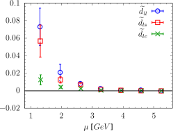
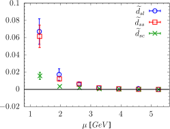
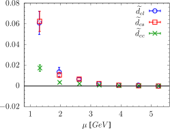
Figure 2: Disconnected projected amputated Green’s function $\widetilde{d}_{\Gamma}^{ff^{\prime}}$ with quark flavors $f$ and $f^{\prime}$ for a scalar bilinear operator $O_{S}^{f^{\prime}}$ at $M_{\pi}=220$MeV ensemble. Here, $\mu^{2}=p^{2}={p^{\prime}}^{2}=(p-p^{\prime})^{2}$ in the RI-sMOM scheme.

2.3 Matching and RG running

At each value of the scale $\mu^{2}=p_{i}^{2}=q^{2}$, the renormalization factors (mixing matrix elements) in RI-sMOM scheme are matched perturbatively [9] to ${\overline{\text{MS}}}$ scheme, $C^{\text{RI-sMOM}\to{\overline{\text{MS}}}}(\mu)=\frac{Z^{\text{RI}}(\mu)}{Z^{\overline{\text{MS}}}(\mu)}$. One of the advantages of using RI-sMOM scheme for the scalar channel is the better convergence in the perturbative series of the conversion factor compared to the RI-MOM scheme [10, 8].

Flavor nonsinglet axial current is conserved and therefore there is no matching from RI to ${\overline{\text{MS}}}$ scheme nor RG running due to the Ward identity. On the other hand, conservation of the flavor singlet current is broken by the chiral anomaly, and the renormalization constant becomes nontrivial at the two-loop level. Here, we use the 3-loop anomalous dimension [11] for the RG running. On the other hand, the matching to ${\overline{\text{MS}}}$ is $1+\mathcal{O}(\alpha^{2})$ [12, 13] and we drop the two-loop contribution that is expected to be subpercent. For scalar and tensor operators, two-loop conversion to ${\overline{\text{MS}}}$ [9] and three-loop running [10, 14] is used.

Remaining dependence on the RI-sMOM scale is removed by fits using the quadratic ansatz,
$Z^{{\overline{\text{MS}}}}(2\mathop{\rm GeV}\nolimits;\mu)=Z^{{\overline{\text{MS}}}}(2\mathop{\rm GeV}\nolimits)+c_{1}\mu^{2}+c_{2}\mu^{4}$. We do not have enough data points at small $\mu^{2}$ where non-perturbative effects can be large. So we make fits with a large lower value of $\mu$, and no longer include a $1/\mu^{2}$ term in the ansatz as was done in Refs. [15, 16].

2.4 Renormalization Strategies $\rm{Z_{1}}$ and $\rm{Z_{2}}$ based on $Z_{\psi}^{q}$

The renormalization constants for the isovector bilinear operators in the RI scheme is given by $Z_{\Gamma}|_{\rm RI}(p)=\frac{Z_{\psi}(p)}{c_{\Gamma}(p)}$, where $\sqrt{Z_{\psi}}$ is the renormalization constant for the fermion field and $c_{\Gamma}$ is the projected amputated connected 3-point function calculated in Landau gauge and defined in Eq. (4).

We calculate $Z_{\psi}$ in two ways, which define the two renormalization strategies $Z_{1}$ and $Z_{2}$:

• $\rm Z_{1}$: $Z_{\psi}$ is calculated from the projected bare quark propagator, $Z_{\psi}(p)=\frac{i}{12p^{2}}\operatorname{Tr}[S_{B}^{-1}(p)\text{$\not\!p$}]$

• $\rm Z_{2}$: We use $Z_{\psi}^{\rm VWI}(p)=c_{V}(p)/g_{V}$, where $c_{V}$ is the projected amputated connected 3-point function with insertion of the local vector operator within the quark state while the isovector vector charge $g_{V}$ is from insertion of the vector current within the nucleon state. Using the vector Ward identity (VWI) $Z_{V}g_{V}=1$ implies $Z_{\Gamma}|_{\rm Z_{2}}=c_{V}/c_{\Gamma}$.

These two strategies were used in Ref. [15, 16] for isovector bilinear operators of light quarks, i.e., $g_{\Gamma}Z_{\Gamma}$ and $Z_{\Gamma}/Z_{V}\times g_{\Gamma}/g_{V}$. Later, they were called $\rm Z_{1}$ and $\rm Z_{2}$ in Ref. [17]. In Ref. [15, 16] we showed that they have different behavior versus $q$ as the various discretization effects are different in $Z_{\psi}$ and $Z_{\psi}^{\rm VWI}$ obtained from $S_{B}(p)$ and $c_{V}(p)/g_{V}$, respectively. Our data show

• For both the light and strange quarks, $Z_{V}|_{\rm Z_{1}}\times g_{V}^{l,{\rm bare}}\to 1$ as $a\to 0$, however the deviation at a given $a$ increases for $m_{l}\to m_{s}$ (a significant mass effect due to discretization) as shown in Fig. 3. Satisfying this relation in the continuum limit implies that renormalization using $\rm Z_{1}$ and $Z_{2}$ will give consistent results.

• Final continuum limit values of nucleon charges and form factors using $\rm Z_{1}$ and $\rm Z_{2}$ agree within the quoted errors [17].

The data for $Z_{\Gamma}$ in ${\overline{\text{MS}}}$ at $2\mathop{\rm GeV}\nolimits$ is shown in Fig. 4 for the $a06m310$ ensemble as a functions of $\mu$ along with a quadratic extrapolation in $\mu^{2}$. The results for the diagonal parts of $Z_{1}$ and $Z_{2}$ show a difference which vanishes in the continuum limit. The off-diagonal mixing elements $Z_{\Gamma}^{u+d,s}$ and $Z_{\Gamma}^{s,u+d}$ shown in the bottom two rows are all smaller than $1\%$ and the $Z_{1}$ and $Z_{2}$ results essentially overlap.

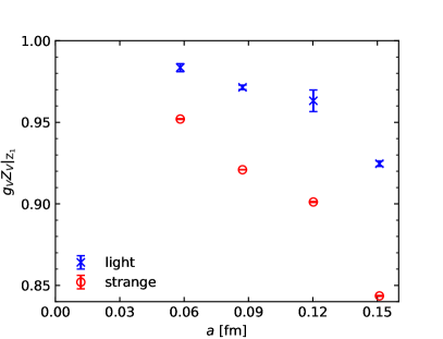
Figure 3: $g_{V}^{f}Z_{V}^{f}|_{\rm Z_{1}}$ for the light and strange valence quark masses. The isovector vector charge $g_{V}^{f}$ is from the forward matrix element with a nucleon state for both quark masses. The vector renormalization factor is $Z^{f}_{V}|_{\rm Z_{1}}=Z_{\psi}^{f}/c^{f}_{V}$ for a flavor $f\in\{l,s\}$. The vector Ward Identity (VWI), $g_{V}Z_{V}|_{\rm Z_{1}}=1$ is likely restored in the continuum limit, however, a linear extrapolation is insufficient.

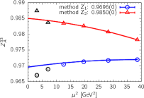
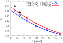
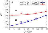
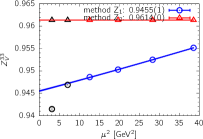
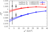
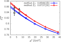
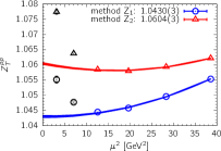
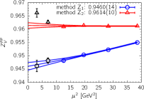
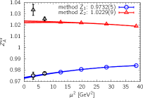
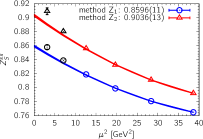
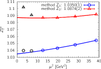
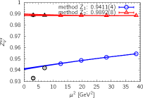
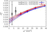
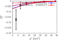
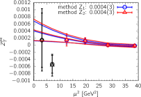
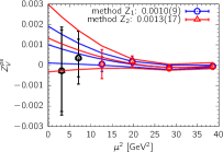
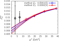
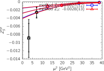
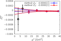
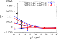
Figure 4: $Z_{\Gamma}$ in ${\overline{\text{MS}}}$ at $2\mathop{\rm GeV}\nolimits$ and quadratic extrapolation in $\mu^{2}$, calculated on a06m310 ensemble. The results from two different strategies, $Z_{1}$ (blue) and $Z_{2}$ (red) are being compared. Each column represents axial, scalar, tensor and vector operator, respectively. Each row represents one of the 5 nonzero matrix elements of $Z$ in $\{u-d,u+d,s\}$ in Eq. (6).

3 Chiral-Continuum-Finite-Volume (CCFV) extrapolation and results

We have carried out four analyses. (i) Standard fits to remove ESC with $Z_{1}$ renormalization. (ii) Fits including $N\pi$ state to remove ESC with $Z_{1}$ renormalization. (iii) Standard fits to remove ESC with $Z_{2}$ renormalization. (iv) Fits including $N\pi$ state to remove ESC with $Z_{2}$ renormalization. For details on ESC fits see Refs. [4, 6].

The renormalized axial, $g_{A}^{u,d,s}$, tensor, $g_{T}^{u,d,s}$, and strange scalar, $g_{S}^{s}$ charges are extrapolated to the physical point, $a\to 0$, $M_{\pi}=135$ MeV, and $M_{\pi}L\to\infty$ using the CCFV ansatz, $g(a,M_{\pi},M_{\pi}L)=c_{0}+c_{a}a+c_{2}M_{\pi}^{2}+c_{3}\frac{M_{\pi}^{2}e^{-M_{\pi}L}}{\sqrt{M_{\pi}L}}$ that includes the leading corrections in all three variables $\{a,M_{\pi},M_{\pi}L\}$. For the scalar charges $g_{S}^{u,d}$, the leading pion mass dependence starts $O(M_{\pi})$ due to the pion loop and a different finite volume correction [4], $g_{S}^{u,d}(a,M_{\pi},M_{\pi}L)=d_{0}+d_{a}a+d_{2}M_{\pi}+d_{3}M_{\pi}^{2}+d_{4}M_{\pi}\left(1-\frac{2}{M_{\pi}L}\right)e^{-M_{\pi}L}$. We ignore higher order terms (chiral logs, etc.) since we only have data at three values of $M_{\pi}$. Results (to be considered preliminary until published) for all four analyses are summarized in Table 1.

Figure 5 shows CCFV fits to $g_{A}^{u}$. The data from two renormalization methods, Z1 and Z2 defined in Sec. 2.4, show different $a$ and $M_{\pi}$ dependence, but the extrapolated results are consistent. This holds for all charges $g_{A,S,T}^{u,d,s}$. Similarly, results from the two excited state fit methods, ‘standard’ and $N\pi$ are consistent for $g_{A,T}^{u,d,s}$, however, there is a significant difference between the ‘standard’ and $N\pi$ results for the scalar charges $g_{S}^{u,d,s}$. Note that the ESC fits to the current data do not distinguish between the two on the basis of $\chi^{2}/dof$ but give different estimates. The large enhancement in $g_{S}^{u,d}$ due to $N\pi$ state contribution is discussed in Ref. [4]. For the strange charges $g_{\Gamma}^{s}$, we do not expect a large contribution from multihadron states since the lowest state is $\Sigma K$, which has a large mass gap ($>N(1440)$), so we consider the ‘standard’ analysis more appropriate than ‘$N\pi$’.

	Standard Method for removing ESC			$N\pi$ method
$q$	$g_{A}^{q}$	$g_{T}^{q}$	$g_{S}^{q}$	$g_{A}^{q}$	$g_{T}^{q}$	$g_{S}^{q}$
u	0.794(29)	0.789(27)	6.48(66)	0.784(34)	0.788(37)	8.8(1.3)
d	-0.385(26)	-0.203(11)	6.09(73)	-0.416(36)	-0.188(17)	8.69(89)
s	-0.051(11)	-0.0016(11)	0.38(12)	-0.066(12)	-0.0016(11)	0.67(16)
u	0.784(30)	0.778(28)	6.45(68)	0.777(34)	0.780(37)	8.9(1.4)
d	-0.381(26)	-0.201(12)	6.09(75)	-0.414(37)	-0.185(17)	8.75(91)
s	-0.053(11)	-0.0015(12)	0.36(13)	-0.069(13)	-0.0015(12)	0.67(17)

Table 1: Preliminary results for flavor diagonal charges of proton (for neutron interchange $u\leftrightarrow d$) with the two strategies used to remove ESC, "standard" and $N\pi$. The top three rows give the results obtained using the $Z_{1}$ renormalization method, and the bottom three with the $Z_{2}$ renormalization method.

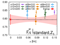
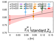
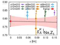
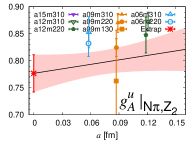
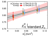
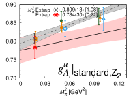
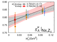
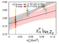
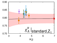
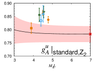
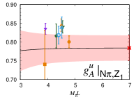
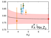
Figure 5: Each column shows the CCFV extrapolation for $g_{A}^{u}$ versus $a$, $M_{\pi}^{2}$ and $M_{\pi}L$ with the other 2 variables set to their physical point values. The rows give the 4 different analyses done: (i) {standard, $Z_{1}$}, (ii) {standard,$Z_{2}$}, (iii) {$N\pi$,$Z_{1}$} and (iv) {$N\pi$,$Z_{2}$}.

4 Conclusions

We have now determined all the nucleon flavor diagonal charges, $g_{A,S,T}^{u,d,s}$, removing previous approximations in renormalization and ESC fits made in Ref. [2, 3], which are shown to be negligible. Further details will be provided in a paper under preparation. A key issue with the ES analysis is the need for a data driven method to distinguish between the ‘standard’ and ‘$N\pi$’ fits, particularly for $g_{A,T}^{u,d}$. To address this limitation, we are increasing the statistics on two physical $M_{\pi}$ ensembles.

References

- [1] MILC Collaboration, A. Bazavov, C. Bernard, J. Komijani, C. DeTar, L. Levkova, W. Freeman, S. Gottlieb, R. Zhou, U. M. Heller, J. E. Hetrick, J. Laiho, J. Osborn, R. L. Sugar, D. Toussaint, and R. S. Van de Water Phys. Rev. D 87 (2013), no. 5 054505, [1212.4768].
- [2] H.-W. Lin, R. Gupta, B. Yoon, Y.-C. Jang, and T. Bhattacharya Phys. Rev. D98 (2018), no. 9 094512, [1806.10604].
- [3] R. Gupta, B. Yoon, T. Bhattacharya, V. Cirigliano, Y.-C. Jang, and H.-W. Lin Phys. Rev. D98 (2018), no. 9 091501, [1808.07597].
- [4] R. Gupta, S. Park, M. Hoferichter, E. Mereghetti, B. Yoon, and T. Bhattacharya Phys. Rev. Lett. 127 (2021), no. 24 242002, [2105.12095].
- [5] Flavour Lattice Averaging Group (FLAG) Collaboration, Y. Aoki et al. Eur. Phys. J. C 82 (2022), no. 10 869, [2111.09849].
- [6] S. Park, T. Bhattacharya, R. Gupta, H.-W. Lin, S. Mondal, and B. Yoon PoS LATTICE2022 (2023) 118, [2301.07890].
- [7] G. Martinelli, C. Pittori, C. T. Sachrajda, M. Testa, and A. Vladikas Nucl.Phys. B445 (1995) 81–108, [hep-lat/9411010].
- [8] C. Sturm, Y. Aoki, N. H. Christ, T. Izubuchi, C. T. C. Sachrajda, and A. Soni Phys. Rev. D80 (2009) 014501, [0901.2599].
- [9] J. A. Gracey Eur. Phys. J. C71 (2011) 1567, [1101.5266].
- [10] K. G. Chetyrkin and A. Retey Nucl. Phys. B583 (2000) 3–34, [hep-ph/9910332].
- [11] S. A. Larin Phys. Lett. B 303 (1993) 113–118, [hep-ph/9302240].
- [12] J. Green, N. Hasan, S. Meinel, M. Engelhardt, S. Krieg, J. Laeuchli, J. Negele, K. Orginos, A. Pochinsky, and S. Syritsyn Phys. Rev. D95 (2017), no. 11 114502, [1703.06703].
- [13] J. A. Gracey Phys. Rev. D 102 (2020), no. 3 036002, [2001.11282].
- [14] J. A. Gracey Phys.Lett. B488 (2000) 175–181, [hep-ph/0007171].
- [15] T. Bhattacharya, V. Cirigliano, S. D. Cohen, R. Gupta, H.-W. Lin, and B. Yoon Phys. Rev. D94 (2016), no. 5 054508, [1606.07049].
- [16] B. Yoon et al. Phys. Rev. D 95 (2017), no. 7 074508, [1611.07452].
- [17] Nucleon Matrix Elements (NME) Collaboration, S. Park, R. Gupta, B. Yoon, S. Mondal, T. Bhattacharya, Y.-C. Jang, B. Joó, and F. Winter Phys. Rev. D 105 (2022), no. 5 054505, [2103.05599].
- [18] SciDAC, LHPC, UKQCD Collaboration, R. G. Edwards and B. Joó Nucl. Phys. Proc. Suppl. 140 (2005) 832, [hep-lat/0409003].