Self-supervised learning for skin cancer diagnosis with limited training data

Abstract

Cancer diagnosis is a well-studied problem in machine learning since early detection of cancer is often the determining factor in prognosis. Supervised deep learning achieves excellent results in cancer image classification, usually through transfer learning. However, these models require large amounts of labelled data and for several types of cancer, large labelled datasets do not exist.

In this paper, we demonstrate that a model pre-trained using a self-supervised learning algorithm known as Barlow Twins can outperform the conventional supervised transfer learning pipeline. We juxtapose two base models: i) pretrained in a supervised fashion on ImageNet; ii) pretrained in a self-supervised fashion on ImageNet. Both are subsequently fine tuned on a small labelled skin lesion dataset and evaluated on a large test set.

We achieve a mean test accuracy of 70% for self-supervised transfer in comparison to 66% for supervised transfer. Interestingly, boosting performance further is possible by self-supervised pretraining a second time (on unlabelled skin lesion images) before subsequent fine tuning. This hints at an alternative path to collecting more labelled data in settings where this is challenging - namely just collecting more unlabelled images. Our framework is applicable to cancer image classification models in the low-labelled data regime.

1 Introduction

Cancer is the second leading cause of death worldwide, with almost 10 million deaths estimated in 2020 [17]. In several types of cancer (e.g. skin, oral, pancreatic), early diagnosis is the major determining factor in prognosis [31, 18, 34]. If cancer is detected sufficiently early, survival rates may be above 90% [52, 33, 69]. On the other hand, the prevalence of several cancer types is increasing [69], and this is particularly true in poorer communities in the developing world [60]. This is of particular concern since individuals in such communities have lower (if any) access to the expert clinicians traditionally needed to diagnose such cancer. There is thus an urgent need to develop cheaper and more data-efficient methods of diagnosis that can be deployed globally. The use of machine learning and artificial intelligence has the potential to provide automated online diagnosis, breaking barriers internationally [13]. Such systems can guide or be leveraged in decision-making of medical practitioners [32] which can provide huge benefits to disadvantaged communities, such as rural areas of developing countries [21].

In recent years, there has been significant interest in applying machine learning to cancer image diagnosis [43]. This includes lung, breast and several other forms of cancer, and involves classifying clinical images into categories (“malign" or “benign") or more fine-grained classification [39, 12, 71]. There have been some challenges in the use of deep learning methods since they require large and class-balanced datasets to function properly. The availability of timely data with proper organisation has been a challenge in the medical domain due to restrictions in archive access given patient confidentiality and ethical approval concerns [64]. In general, the collection of labelled datasets is a nontrivial issue and requires significant time and money to collect and annotate [11]. This is even more pronounced for medical images, which require expert knowledge or even medical testing (e.g. via biopsy) to classify, dramatically increasing the cost [27, 10]. Thus for several types of cancer, image datasets suitable for machine learning research are lacking. For example, Sengupta et al. [56] demonstrated that there is a dearth of publically available oral cancer datasets. Although there has been published research on oral cancer image classification, the data used is closed source - our attempt at obtaining data by contacting primary authors was not successful. Oral cancer is diagnosed through biopsy, but the decision to biopsy is made by visual inspection of the mouth [5], and early detection is crucial for prognosis. In the United States, the 5-year survival with early detection is 85%, but only 28% of cases are detected at this stage. In later stages, when cancer has spread, 5-year survival drops to 40% [7]. The lack of available datasets is concerning given that the prevalence of oral cancer is increasing, [69] particularly among poorer parts of the developing world, where expert medical care is less available. As an additional point, certain kinds of cancer have extremely low prevalence. For example, Chordoma has a prevalence of only 0.18-0.84 per million [2], so constructing a large labelled dataset in such cases is a long way off. Developing more data-efficient techniques is therefore essential.

One oral cancer study is by Song et al [60]. The dataset in their study involved 3851 cheek mucosa images, labelled into 4 categories (2417 normal, 1100 premalignant, 243 benign, 91 malign). Like other work, they utilised a network pre-trained from ImageNet as their backbone model, fine-tuning it on the current dataset. The baseline accuracy of this model was 81% whereas the baseline balanced accuracy was 62%. The reason for this discrepancy is that the dataset is not balanced. To improve the performance the authors use a combination of undersampling of the majority class and oversampling of the minority classes (through data augmentation). After doing so the accuracy is still 81% but the balanced accuracy increased to 80%. Brinker et al. [6] considered a balanced training set of 4204 melanoma and nevi mole images, where the classification had been determined by biopsy. Note that although this training set is smaller than other studies, it is a binary classification problem. They also utilised a transfer learning approach, via a ResNet-50 pre-trained on ImageNet. On the metrics of sensitivity and specificity, they found that the trained network outperformed dermatologists. The sensitivity and specificity were around (67.2%, 62.2%) for dermatologists and (82.3%,77.9%) for the neural network, a significant margin.

Typically, supervised deep learning involves first randomly initialising the weights of a neural network, and then iteratively updating the weights through backpropagation and stochastic gradient descent [19]. A very well-known problem with this approach is that for challenging high-dimensional problems, large amounts of labelled data are required to achieve good performance. Transfer learning is a machine learning technique that attempts to solve this problem. The idea is to initialise the neural network weights with those of a network that has already been trained (traditionally in a supervised fashion) on a related task [75]. A common strategy in computer vision applications is to take the initial network to be one that has been pre-trained on ImageNet [75]. It has been demonstrated that transfer learning can lead to significant performance gains compared to training from random initialisation [61].

Self-supervised learning (SSL) is a machine learning technique that involves training a model on unlabelled data in order to learn a good internal representation for downstream tasks [30]. The model uses the data itself to develop a surrogate target, which is the main distinguishing feature from unsupervised learning, although the boundary is not well defined. With this definition, denoising autoencoders [67] would be self-supervised models, whereas principal component analysis (PCA) [48] is unsupervised but not self-supervised. SSL has had huge success in natural language processing (NLP) problems such as language translation, topic modelling and sentiment analysis[42]. At a high level, the approach is to take an input sentence (or sequence) and “blank out" some of the text. The goal is to predict the missing text from the available text, usually using a transformer architecture and trained in an autoregressive fashion [66, 41]. Hence, large language models such as generalised pre-trained transformers (GPT-x) [50], and machine translation engines [70] such as Google Translate are based on self-supervised learning. SSL has historically been less successful in computer vision tasks [41], since visual images are inherently of much higher dimension. It is possible to represent a probability distribution over words exactly (there are $\sim$ 60k words in the English language), but doing this for natural images remains a challenge [41]. Despite this, in the last few years a particular form of SSL known as ‘joint embedding architecture’ applied to computer vision tasks has had significant success [23, 74, 20], rivalling supervised approaches in some cases. Therefore, SSL has a huge potential for medical diagnosis that has image data with certain limitations such as class imbalance and limited training data.

The use of transfer learning is common in the medical diagnosis literature concerning images [75] such as skin cancer [36] and lung cancer diagnosis [68]. Usually, the models involved have been pre-trained on ImageNet in a supervised fashion. This raises the question - can we do better? Since many studies are based on this framework, any improvement has significant clinical implications. This is of particular interest in the low data regime.

In this paper, we apply SSL and transfer learning to the problem of skin cancer diagnosis based on image data, which is imbalanced and has a limited set of training data. We compare models pre-trained the usual way via supervised learning on ImageNet, to networks pre-trained through self-supervised learning, also on ImageNet. We use International Skin Imaging Collaboration (ISIC) [28] image-based dataset with a training set of 2554 instances and a test set of size 19423 instances.

The rest of the paper is organised as follows. Section 2 gives background on deep learning models, transfer learning and self-supervised learning. Section 3 gives details of the methodology with data and framework that features self-supervised learning. Section 4 presents the results, Section 5 discusses the results and highlights the contributions and limitations, and Section 6 presents the conclusion of the paper.

2 Background and Related Work

2.1 Convolutional Neural Networks

Convolutional neural networks are feedforward networks built by stacking convolution layers, max-pooling layers and standard fully connected layers [40]. Convolution layers are the main innovation of CNNs and are motivated by the notion of receptive field in visual neuroscience [26]. Such layers involve several filters each of which are convolved across the input, taking the Frobenius inner product with each region. These outputs are then stacked into channels. If the input to the layer has shape $n\times m\times c$ (e.g. an input image of shape $n\times m$ with $c$ colour channels), and there are $f$ filters of shape $a\times b$ then the output of the layer will have shape $((n-a)+1)\times((m-b)+1)\times f$. (This assumes zero padding and a sliding window of 1). In this way, convolution layers use far fewer parameters than fully connected layers, and CNNs can be seen as a regularised version of the multi-layer perceptron. Max pooling layers downsample their input, but with the innovation of skip connections are not used as much in such residual architectures [24].

2.2 ImageNet

ImageNet is a large annotated database of over 14 million natural images [63]. ImageNet 1k is a subset of about 1.2 million images distributed across 1000 categories [53, 11]. (Henceforth, when we refer to ImageNet we mean ImageNet 1k). Some example categories are ‘magpie’, ‘taxi’, and ‘crane’. In transfer learning applications it is common to take the initial network to be one trained on ImageNet in a supervised fashion [61]. The size of the dataset along with the large number of categories means such networks must learn informative features in order to perform ImageNet classification. Transfer learning is discussed more in the following sections.

2.3 Residual networks

The backbone architecture used in our experiments is a ResNet-50, which is a residual CNN with 50 layers. Residual networks were motivated by the curious empirical finding that adding a sufficient number of layers to a deep network eventually led to an increase in training error, as well as test error [24]. Hence the test error increase is not due to overfitting alone. Note that if the additional layers simply learned an identity function, then the deeper network can learn the same function as a shallower network.

A solution to this problem is the introduction of residual skip connections, as depicted in 1. The output $x$ of an earlier layer is input to the next layer and is also added to the output of a later layer. If the dimensionality of the additions does not match, the identity mapping in 1 may be replaced by a matrix multiplication $W$ with learnable parameters. Part of the motivation for this block is that it is easier to learn an identity function by driving $\mathcal{F}$ to the zero function than by modelling an identity function explicitly. Said another way, if the function we want to learn is $\mathcal{G}$, then it is easier to infer it from data by modelling the residual:

$$\mathcal{F}(x)\equiv\mathcal{G}(x)-x.$$

Kaiming et al. [24] demonstrated that the introduction of residual blocks enabled stable training of deeper networks, and state-of-the-art performance on ImageNet in 2015. Their seminal paper is the most cited neural network paper of this century.

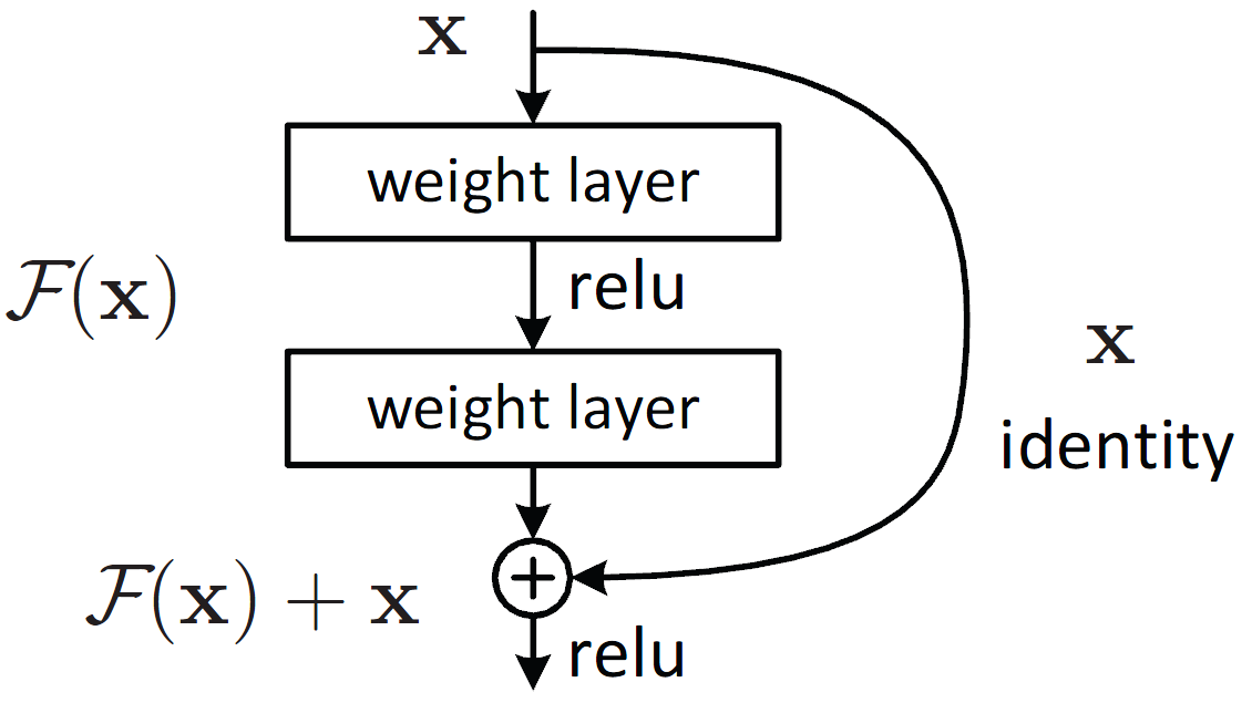
Figure 1: A residual block [24]

2.4 Image-based cancer diagnosis

2.4.1 Skin cancer detection

The ISIC database is a large database of skin lesion images that have been carefully curated by experts [28]. The ISIC2018 training dataset had 10015 images, distributed among 7 categories (melanoma, basal cell carcinoma, melanocytic nevus, dermatofibroma, benign keratosis, actinic keratosis, and vascular lesion). As an example of work on this data, Guo and Ashour [22] took a supervised transfer learning approach, utilising CNNs pre-trained on ImageNet. Their model had an AUC of 72 on a validation set. In other work Majtner et al. [44] fine-tuned two models on the 10015 labelled ISIC examples. The network architectures were VGG16 and GoogLeNet and had both similarly been pre-trained on ImageNet. The individual accuracy of the nets was 80.1% and 79.7% and the accuracy of the ensemble was 81.5%.

Maron et al. [45] trained a network on 11444 ISIC skin images. The architecture is a ResNet-50 pre-trained on ImageNet. They evaluate the model on a test set of biopsy-determined images under two tasks: classification into benign and malign; and classification into the correct category among 5 possibilities. They compare the performance to that of 112 dermatologists and find that it is generally superior. For the first task, the sensitivity and specificity for dermatologists was 74.4% and 59.8%. For the same sensitivity, the specificity of the CNN was 91.3%. On the second task, the performance of the network is superior except for the basal cell carcinoma category where it is on par. The accuracy of dermatologists for melanoma is 63% vs. 65% for the network.

Indeed, it is at this point known that deep learning can outperform dermatologists, given a large labelled dataset. Esteva et al. [15] trained an Inception v3 CNN on a huge dataset of 129450 lesion images with 2032 disease categories (e.g. instead of a label of ‘melanoma’ there is a more fine-grained subclassification of amelanotic melanoma, lentigo melanoma etc). The network has been pre-trained on ImageNet, and they fine-tune all layers using the RMSProp optimiser, with an initial learning rate of 0.001 which is decayed every 30 epochs. They evaluate the network in several ways and compare its performance to that of dermatologists. On the 3-class classification problem (benign, malign, non-neoplastic) the CNN has an accuracy 72.1% whereas the dermatologist’s mean accuracy is 65.78%. They also compare the performance on two binary classification problems: malignant melanoma v.s. benign nevi; and keratinocyte carcinoma vs. seborrheic keratosis. The CNN generally outperforms the dermatologist’s mean performance on these problems as well.

2.4.2 Other medical diagnosis problems

Singh et al. [55] compared 6 deep learning model architectures (VGG16, VGG19, ResNet-50, DenseNet, MobileNet and EfficientNet) on the problem of breast image classification. The models had all been pre-trained on ImageNet. The derived training dataset under consideration contained 31393 samples and the test set had 7849 samples, relatively balanced between malign and benign. The VGG19 performed best, with sensitivity and precision of 93.05% and 94.46% respectively.

Ayana et al. [1] studied the problem of mammogram classification. Their study is on the DDSM dataset which contains 13128 images, 5970 benign and 7158 malign. They use an 80:20 train-test split. While other literature discussed utilises CNN base architecture (as is typical in medical classification), Ayana et al. instead use vision transformers. They train 3 different transformer architectures: ViT, Swin-T, and PVT. They compare the performance of these models under two regimes: training from scratch, and transfer learning. The transfer learning regime means the weights come from a network pre-trained on ImageNet, as usual. Under the TL regime, all architectures achieve 100% accuracy. Conversely, when training from scratch the performance ranges from 72% - 78%, a huge difference. They also demonstrate that on this problem the vision transformer outperforms several CNN architectures, and so is worthy of further study. Wang et al. [68] applied transfer learning to computerized tomography (CT) lung scan classification, using residual CNNs. The training set has 2054 images distributed among 4 categories, and the test set has 168 images. They also utilise a pre-trained network, but contrary to all other work mentioned, it is not pre-trained on ImageNet. Rather, it has been pre-trained on another lung image dataset (Luna16) and achieved 85.71% accuracy.

Khan et al. [35] applied transfer learning to the problem of Alzheimer’s disease multiclass classification from magnetic resonance imaging (MRI) images. There are four categories: healthy controls, early mild cognitive impairment, late mild cognitive impairment and Alzheimer’s disease. The dataset has a range of 1882-4637 slices per category, with 70% for training and 15% for testing. ImageNet pre-trained VGG16 and VGG19 networks were used where the backbone models were frozen and several fully connected layers were appended to the networks. Hence they follow the ‘linear evaluation’ protocol (see 2.5) except the head is nonlinear instead of linear. The head consists of fully connected layers of sizes $(4096,1000,512,4)$. The VGG19 performs slightly better than the VGG16 network, with accuracies of 98.47% and 97.12% respectively. They demonstrate that these networks are superior to several alternative architectures, such as AlexNet and ResNet-50.

Baldota et al. [3] study the problem of pancreatic cancer classification. Their study involves a large dataset of size 26469 among three categories: healthy, cancer and pancreatitis. An ImageNet pre-trained DenseNet201 is fine tuned resulting in almost 100% accuracy of 99.87%. This study demonstrates the performance that is possible with a sufficient amount of labelled data.

Jabbar et al. [29] studied the problem of diabetic retinopathy classification. The training set had 35126 samples among 5 categories: normal, mild, moderate, severe, proliferative. They compare several ImageNet pre-trained networks, for which the accuracy ranges from 92.4% to 96.6%.

We can summarise that all the mentioned studies involved transfer learning. Specifically, the initial neural networks were pre-trained in a supervised fashion, usually on ImageNet and with a CNN base architecture. In later sections of this paper, we discuss an alternative pre-training methodology called self-supervised learning, which can yield superior transfer results.

2.5 Transfer learning

A common strategy in computer vision applications is to take the initial network to be one that has been pre-trained on ImageNet. The final linear layer (which represents the scores for the 1000 ImageNet categories) is removed and a new linear layer is appended mapping to the correct number of categories for the present task. This ‘supervised transfer learning’ approach consistently outperforms training from random initialisation [61].

Transfer learning can be motivated based on insights into how humans learn. Knowledge in one domain can be used to assist learning in a new but related domain. This may exist on a cognitive level or a motor level. For example, visual knowledge required to identify horses can be used to identify zebras; or motor knowledge of how to play softball can be used to play baseball. Pan and Yang provide a formal definition of transfer learning in terms of probability distributions [46], see also [36].

The success of transfer learning in deep learning can also be understood by analogy with the primate visual system. Early layers of the visual cortex are tuned to detect generic features of objects, such as edges. High-level semantic knowledge happens at higher cortical levels [26]. Similarly, early layers of supervised CNNs tend to learn features resembling colour blobs or Gabor filters, and this appears to be independent of the data they are trained on [72]. The final layers, conversely, are more tuned to the specific supervised problem at hand. Indeed, consider the last layers output representing the scores (normalised or unnormalised) for the categories under consideration. Permuting the labels (e.g. dog=0, cat=1 $\rightarrow$ cat=0, dog=1) does not change the nature of the classification problem. In this case, the trained network can remain the same except for the multiplication of the final layer by a permutation matrix.

There are several ways to perform transfer learning. Three examples are:

1. Freeze the pre-trained model and train only the new linear layer. This is known as a linear probe or linear evaluation.

2. Do 1. for several iterations, and then unfreeze the backbone model and continue training as usual.

3. Train the network the standard way (no freezing involved).

If the distribution of the current dataset is similar to the pre-training distribution, then it is well known that 3. is superior to 1. In this case, standard fine-tuning outperforms a linear probe. However, if the distributions are not similar Kumar et al. [38] demonstrated that 1. can outperform 3. Generally, 2. is superior overall. The problem with 3. in the out-of-distribution setting is that the pre-trained model contains high-quality features which may be destroyed at the start of training by aligning the body of the network with the head (with respect to the new dataset). This is a problem because the head is randomly initialised. Training the head only, with the backbone frozen for $\sim 1$ epoch is typically sufficient to align it with the body with respect to the current data so that the pre-trained features are not lost. Hence we follow scheme 2. in this work.

2.6 Self-supervised learning and Barlow Twins

For the purposes of this paper, self-supervised learning is a way of pre-training models for transfer learning, but without using label information. The goal is still to learn a model initialisation of a deep network $f_{\theta}$ as in standard (supervised) pre-training. The difference in self-supervised pre-training is that only unlabelled image data is needed. A way this can be done is through a joint embedding architecture [41] which can be seen in 2.

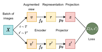
Figure 2: Joint embedding architecture

The joint embedding architecture is a way of performing self-supervised learning. It requires a designated network $f_{\theta}$ which will be the pre-trained model and an unlabelled image dataset. The training process is as follows.

1. Sample a batch of data $X$.

2. Sample two random data augmentations $t\sim T$ and $t^{\prime}\sim T^{\prime}$ and produce two distorted copies of the batch, $v=t(X)$ and $v^{\prime}=t^{\prime}(X)$. For example, each element of the batch may have some random amount of blur applied.

3. Compute the projected representations $z=p(f(v))$ and $z^{\prime}=p(f(v^{\prime}))$.

4. Compute a loss function $\mathcal{L}(z,z^{\prime})$. Update the weights with backpropagation and stochastic gradient descent. Return to step 1 and repeat until convergence.

Once training is completed, the projector is removed, while the encoder is retained - this is the pre-trained model. The loss function could also be computed in encoder space but this leads to inferior representations, see [9].

Barlow Twins is a self-supervised learning algorithm based on this framework. Essentially, it is a way of writing down the loss function in 2. First, the branches $z$ and $z^{\prime}$ are normalised along the batch dimension. The mean (for the first branch) is computed as $\mu_{i}=\frac{1}{n}\sum_{k=1}^{n}z_{ki}$ where $n$ is the batch dimension and similarly the standard deviation: $\sigma_{i}=\sqrt{\frac{1}{n}\sum_{k=1}^{n}\left(Z_{ki}-\mu_{i}^{A}\right)^{2}}$. The normalisation is then computed as $z_{ji}\leftarrow\frac{z_{ji}-\mu_{i}^{A}}{\sigma_{i}^{A}}$. This normalisation is performed analogously for $z^{\prime}$. Next, the cross-correlation between the branches is computed, which is a simple matrix multiply: $\mathcal{C}=\frac{1}{n}(z^{\prime})^{\top}z.$ The Barlow Twins loss function then sets this matrix to the identity matrix:

$$\mathcal{L_{BT}}=\sum_{i}(\mathcal{C}_{ii}-1)^{2}+\lambda\sum_{i\neq j}\mathcal{C}_{ij}^{2}$$ (1)

where $\lambda$ is a hyperparameter. One can think of the loss as being composed of two terms: the first term is an invariance term and the second term is a redundancy reduction term. We encourage the reader to consult [74] for more details regarding the motivation for this loss function, as well as further details on self-supervised learning. For a general introduction to self-supervised learning, see also [41].

The Barlow Twins algorithm has several properties that make it potentially more applicable in the low data regime. For example, Barlow Twins achieves state-of-the-art performance in semi-supervised learning with limited data. As an additional point, Barlow Twins can be trained with batches as low as 128, in contrast to other self-supervised methods which may need batches in excess of 4000 to work well [9]. This is helpful in the case that a limited compute budget is available, e.g. using very large batches may not be possible due to memory limitations.

3 Methodology

3.1 Data

Skin lesion classification is a well-studied problem, and as discussed it is possible to train models that outperform human experts [6] which is primarily due to the existence of large labelled datasets. The existence of large datasets is not available for all types of problems and hence our work is motivated by cases where such datasets do not exist, such as oral cancer. Our model training set only has 2554 samples which make less than 12% percent of total data, more closely mirroring the oral cancer study in [60] which had 3851 training samples among 4 categories. Note that over 90% of oral cancer cases are squamous cell carcinomas [69].

Lesion type	Train	Test
Actinic Keratosis	306	498
Basal Cell Carcinoma	500	2549
Benign Keratosis	467	1663
Dermatofibroma	55	173
Melanoma	500	3339
Nevus	500	10601
Squamous Cell Carcinoma	171	414
Vascular Lesion	55	186
Total	2554	19423

Table 1: Number of samples in the training and test set, per lesion type.

The data comes from an open-source dataset, ISIC2019 [62] which includes ISIC2018 as a subset. This is a labelled skin lesion dataset. There are 8 lesion categories, 4 of which are benign, that is not cancerous (benign keratosis, dermatofibroma, nevus, vascular lesion) with the remainder being malign, that is cancerous or pre-cancerous. The category actinic keratosis is precancer, whereas basal cell carcinoma, melanoma, and squamous cell carcinoma are all cancerous. There are only 171 squamous cell carcinoma samples, making this a very challenging dataset.

3.2 Framework

The general transfer learning procedure can be seen in the "fine tune" component of our framework in Figure LABEL:fig:framework. Also see the earlier section on transfer learning 2.5 for background. First, the pre-trained encoder is frozen and the linear head is fit for 1 epoch against the frozen representation. This is essentially multinomial logistic regression on $x^{\prime}=f_{\theta}(x)$ with $\theta$ frozen. Next, the encoder is unfrozen and we run a learning rate finder to find a good maximum learning rate $lr$ to use. Lastly, we train the whole network for 40 epochs using the 1cycle policy and maximum learning rate $lr$. The Adam optimiser is used at all stages [37]. We explain all steps of the algorithm in detail in the following sections. Step 4. is essentially a hyperparameter search and step 5. is the main training loop, both discussed in detail in the implementation section, including background information.

In the "fine tune" component of our framework in Figure LABEL:fig:framework, it does not matter much how the linear layer is trained as the point is just to align the head with the encoder, so the pre-trained representations are not harmed in subsequent learning. Moreover, learning rate schedules are more essential for deep networks, and when training for multiple epochs. We use the Adam optimiser [37] with a fixed learning rate of 0.001.

We apply the transfer learning methodology in our framework in Figure LABEL:fig:framework across two kinds of initial weights: supervised and self-supervised. The supervised initial weights have been pre-trained on ImageNet in a supervised fashion; i.e. the network has been trained with cross-entropy to predict class labels out of 1000 total classes [49]. The self-supervised initial weights have similarly been pre-trained on ImageNet but using the Barlow Twins algorithm [51]. Note that no labels are used in this algorithm. The initial weights both come from the same backbone architecture, a ResNet-50. This is a convolutional neural network with 50 layers, with residual connections between layers. The penultimate layer of a ResNet-50 has dimensionality 2048, and we call the network up to this penultimate layer the ‘encoder’, denoted $f_{\theta}$. For the supervised network, the final layer is a linear layer with an input dimension of 2048 and an output dimension of 1000. This last linear layer is removed, and a newly initialised linear layer is appended to the network, with the correct shape (input dimension 2048, output dimension 8 for the number of lesion categories). The Barlow Twins network involves a ResNet-50 encoder, followed by several projector layers: $P\circ f_{\theta}$. The projector network is removed, and a linear layer is similarly appended. Hence, the initialised models have the form: $Linear_{8}\circ f_{\theta}$.

3.3 Implementation

The ISIC images are of varying dimensions, but neural networks require an input of homogeneous dimensionality. Therefore, we resize the data to $256\times 256$. A batch size of 64 is used to suit our deep learning models. During training, each time a mini-batch is sampled we apply random data augmentation before passing it through the network. Each element of the batch is randomly cropped, rotated and flipped. The rotation is by a random angle in $[0,45]$ degrees, and the resize scale and resize ratio for cropping are $(0.7,1.0)$ and $(0.75,1.33)$, respectively.

	Crop	Flip	Rotate
Probability	1.0	0.25	0.25

Table 2: Probabilities for augmentations.

Data augmentation done in this way during supervised learning is a standard strategy to prevent overfitting. The models sees several slightly different views of each image during training. This procedure can be seen in Figure 4. Each column represents a minibatch of size 2, with data augmentation applied. This is an example of different views of the same data presented to the model during training.

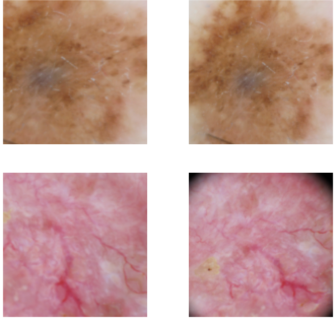
Figure 4: Train and test augmentation

Test time augmentation is another strategy to improve generalisation, closely related to the above technique [57]. The standard way of computing probabilities at test time is to take the test data, pass it through the neural network, and return an output probability through a softmax layer. Test time augmentation simply repeats this process several times, for augmented views of the test data. This will return several probabilities for each test input, which are then averaged to get the final probability. For example, in Figure 4, test time augmentation would compute the probabilities for each column the standard way, and then average the probabilities. This is because the columns represent the same data but under different augmentation. We use exactly the same augmentations as during training, i.e. as in Table 2, and compute the average across three probabilities for each test input. Predictions are then made by taking the argmax of these probabilities, as usual.

The 1cycle training policy is a learning rate and momentum scheduler [59, 58]. It involves starting training with a very low learning rate $l_{1}$ which is then increased up to a maximal learning value $l_{2}$. Next, the learning rate is slowly decreased to $l_{1}$, and for the last several epochs, to a much lower final learning rate $\frac{l_{1}}{K}$, where $K>>1$. In other words, the learning rate has an increasing period, from $l_{1}$ up to $l_{2}$, followed by a decreasing period down to $\frac{l_{1}}{K}$. The momentum is also scheduled, but inversely to the learning rate. Momentum decreases at the start of training, to a minimum, then is increased to a maximum. The scheme is most easily understood pictorially and can be seen in LABEL:fig:fitonecycle.

The 1cycle schedule diverges from standard approaches, which predominantly involve learning rate decay - starting at the maximal learning rate and decreasing to a minimum [73]. Smith [58] showed that increasing the learning rate rapidly at the start of training has a regularising effect. It has also been found that when using this policy other forms of regularisation must be reduced - hence we do not consider dropout and similar techniques in this work. Moreover, the policy has a particular advantage when the amount of training data is limited, making it especially suited to our purposes.

An important hyperparameter in the 1cycle policy is the maximal learning rate (i.e. the peak in LABEL:fig:fitonecycle). In fact, this hyperparameter can be automatically inferred. A learning rate finder launches a mock training session and trains the model for several iterations, increasing the learning rate each time and recording the loss. The learning rate starts at a very low value and increases to a high value. A representative plot of this procedure can be seen in LABEL:fig:lr_im. The loss will decrease at the start, before eventually increasing (or perhaps oscillating). A maximal $lr$ is chosen that is somewhere in between a sharp valley and the minimum.

4 Results

4.1 Comparison of supervised transfer and self-supervised transfer

We ran multiple experiments in model training (i.e. trained 35 models with different weight and bias head initialisation), against two different backbone models. The backbone models have the same architecture, but different initial weights. The framework section provides extensive detail about this model fine-tuning procedure 3.2. The fine-tuning is done through algorithm LABEL:algorithm_transfer.

Therefore, the initial weights of the backbone models were either from a ResNet-50 pre-trained in a supervised manner on ImageNet; or from a ResNet-50 pre-trained in a self-supervised manner (with Barlow Twins) on ImageNet [49, 51]. We call these ‘supervised models’ and ‘self-supervised models’ respectively, which simply refers to how the initial weights were generated. Table 3 shows 0.663 mean test accuracy of the supervised models and 0.703 mean accuracy of the self-supervised models. This demonstrates the strength of using self-supervised transfer learning in the domain of cancer image classification.

	Supervised	Self-supervised
Mean Accuracy	0.663	0.703
Standard Deviation	0.0198	0.014
Number of Models	35	35

Table 3: Model fine-tuning results for two kinds of initial weights.

Also displayed is the mean F1 score, for each lesion type. This can be seen in 4. We calculate the F1 score for each of the 35 runs and then display the average value. The supervised models had a mean weighted average of 0.68, v.s. 0.71 for self-supervised. Moreover, self-supervised models had a larger F1 score for every lesion category, although the difference was not always large. Of particular note, the largest F1 differential among the malign categories was for squamous cell carcinoma, with self-supervised 10.8% higher than supervised. Squamous cell carcinoma also had the lowest training support, with only 171 samples. Displayed in two separate tables are the precision and recall values for each category, across the initial weights. These are also the mean values across 35 runs.

Lesion Type f1-score(sup) f1-score (self-sup) Support Actinic keratosis 0.44 0.45 498 Basal cell carcinoma 0.72 0.73 2549 Benign keratosis 0.48 0.49 1663 Dermatofibroma 0.33 0.37 173 Melanoma 0.56 0.57 3339 Melanocytic nevus 0.77 0.82 10601 Squamous cell carcinoma 0.35 0.39 414 Vascular lesion 0.31 0.51 186 Weighted avg. 0.68 0.71 19423 Accuracy 0.66 0.70 19423

Table 4: Combined classification report for skin lesion classification model. Each value is a mean across 35 runs.

Lesion Type precision recall f1-score support Actinic keratosis 0.36 0.57 0.44 498 Basal cell carcinoma 0.70 0.76 0.72 2549 Benign keratosis 0.47 0.49 0.48 1663 Dermatofibroma 0.37 0.30 0.33 173 Melanoma 0.50 0.63 0.56 3339 Melanocytic nevus 0.85 0.70 0.77 10601 Squamous cell carcinoma 0.36 0.34 0.35 414 Vascular lesion 0.25 0.67 0.35 186 Weighted avg. 0.70 0.66 0.68 19423 Accuracy 0.66

Table 5: Supervised weights. Mean classification report

Lesion Type precision recall f1-score support Actinic keratosis 0.37 0.57 0.45 498 Basal cell carcinoma 0.70 0.75 0.73 2549 Benign keratosis 0.49 0.50 0.49 1663 Dermatofibroma 0.43 0.32 0.37 173 Melanoma 0.52 0.63 0.57 3339 Melanocytic nevus 0.86 0.78 0.82 10601 Squamous cell carcinoma 0.48 0.34 0.39 414 Vascular lesion 0.53 0.51 0.51 186 Weighted avg. 0.72 0.70 0.71 19423 Accuracy 0.70

Table 6: Self-supervised weights. Mean classification report.

Also displayed are two representative ROC curves. Note that the test set has 19423 samples so is only balanced with respect to the nevus category which has 10601 test examples. In all the other categories, there is class imbalance. The ROC is generally not as meaningful in such a setting, (see for example [54], ROC tends to overestimate performance in the imbalanced data setting) which is why we emphasise the earlier results, but is included here for completeness.

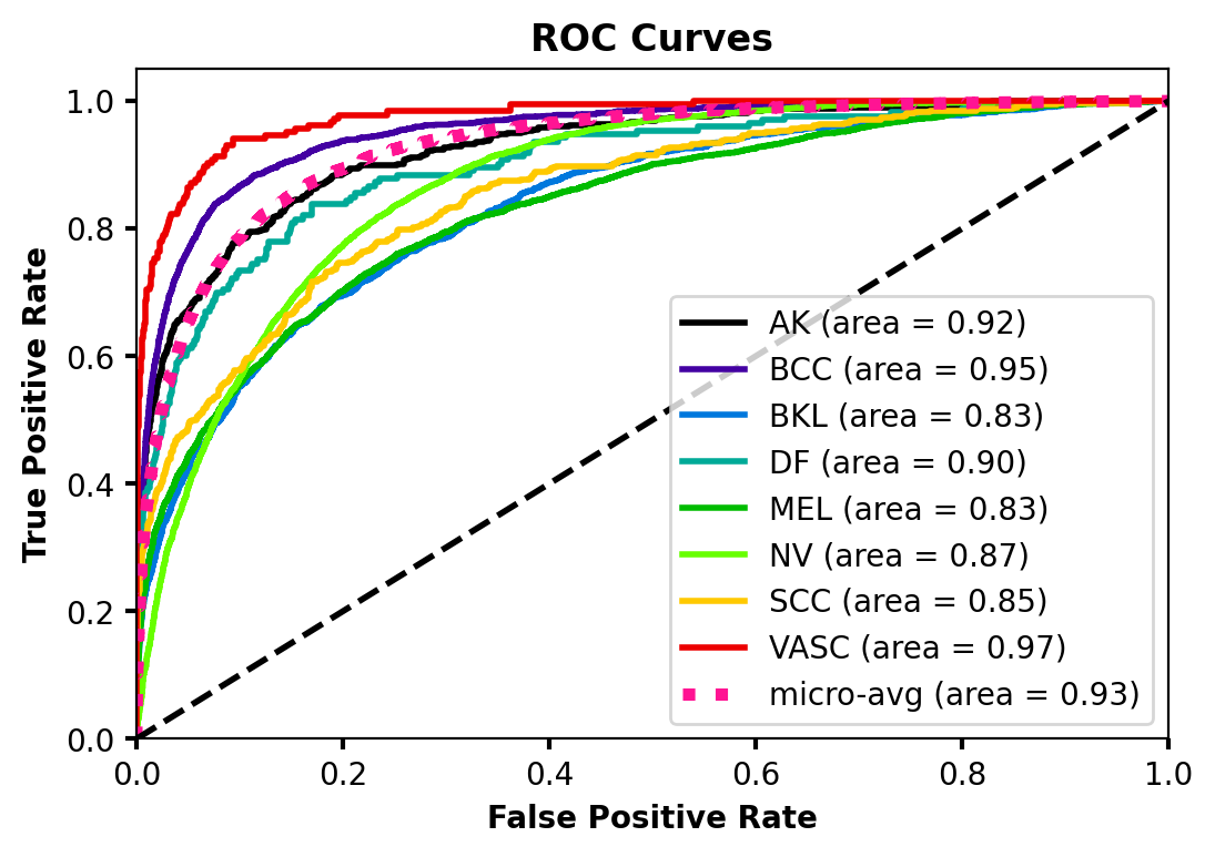
Figure 7: A representative ROC curve for supervised initial weights. The model displayed had a test accuracy equal to the mean of 0.66.

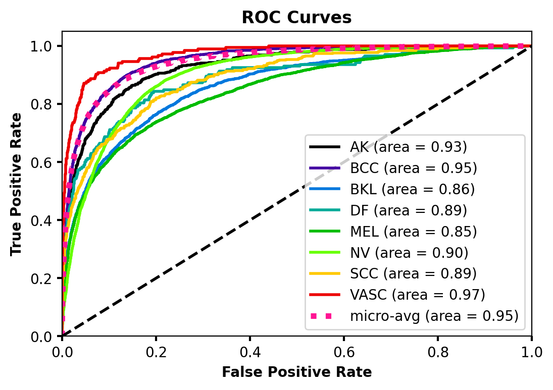
Figure 8: A representative ROC curve for the Barlow Twins model initial weights. The model displayed had a test accuracy equal to the mean of 0.7.

Despite demonstrating the superiority of SSL-transfer over supervised transfer, the performance is still not acceptable for clinical applications. In the SSL setting, we keep the amount of labelled data fixed and apply two strategies to improve performance, i.e. 1.) use a larger network, 2.) pre-train on more unlabelled data beyond ImageNet.

4.2 Larger model

Unfortunately, there are no open-source pre-trained Barlow Twins models larger than a ResNet-50. However, there exist larger models pre-trained with VICReg [8]. VICReg is a self-supervised learning algorithm that is very similar to Barlow Twins - and also performs similarly on ImageNet transfer (54.8% semi-supervised accuracy on 1% labels vs. 55% for Barlow Twins) [4]. To establish a baseline, we first fine-tuned a VICReg pre-trained ResNet-50 [8]. Test accuracy was 0.7, exactly in line with the mean accuracy of Barlow Twins. This shows that VICReg performs similarly to Barlow Twins on the present data, just as on ImageNet. Next, we fine-tuned a ResNet-200 (x2) [8] that had also been pre-trained with VICReg on ImageNet. This network has encoder dimension 4096 and 250 million parameters, v.s. 23 million parameters for a ResNet-50. It is therefore a much larger model. Somewhat surprisingly, test accuracy was the same at 0.7. Therefore, the performance of these models (Barlow Twins and VICReg) is saturated with respect to ImageNet pre-training with the ResNet architecture class.

4.3 Pre-training on target data

Next, we consider whether pre-training on more unlabelled data beyond ImageNet can provide better results. More specifically, since we have access to a large quantity of unlabelled data we consider pretraining the (already SSL pretrained) encoder weights a second time - this time on the target data - before subsequent fine tuning as usual. To this end we combined the train and test sets for a total of 21977 unlabelled samples and pre-trained an encoder using Barlow Twins. Similarly to before, Pytorch and FastAI were used along with self_supervised library [65]. We reinitialised a new projector head with 3 layers, all of size 8192. Hence the model to be trained had the form: $P\circ f_{\theta}$ with $P$ a randomly initialised projector and $f_{\theta}$ a ResNet-50 encoder that had already been pretrained with Barlow Twins on ImageNet. We set the hyperparameter $\lambda=\frac{1}{8192}$ (see 1) and the augmentations used were similar to previous papers [74, 20]. The full details are on GitHub. We applied all augmentations with the same probability as [74, 20] and in the same order. Generally, the level of augmentations applied (amount of blur, jitter etc) was the same. A difference was several of the augmentations had a ‘same_on_batch’ parameter, which is set to ‘False’. This means, for example, the amount of blur applied to a batch varies across the batch, rather than being constant.

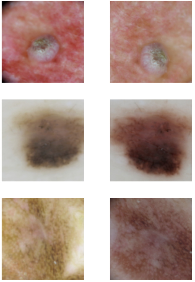
Figure 9: Barlow Twins augmentations. Each row has two distorted views of the same sample.

The batch size was lowered from 1024 (which was used when training on ImageNet) to 128 due to memory limitations [74]. The encoder was frozen for one epoch while updating the projector, analogous to training the head only in supervised transfer learning. We then unfroze the encoder and trained the whole network for 100 epochs using the 1cycle policy. Hence we use the same scheme as in algorithm LABEL:algorithm_transfer with the projector taking the place of the head. The resulting network is then fine-tuned as usual. This whole process is repeated 6 times. We perform this procedure 6 times rather than 35 for two reasons. Firstly, the pre-training step takes far longer training time compared to just fine-tuning as there are 21977 unlabelled samples. Secondly, the results are anyway extremely stable across the 6 runs.

Supervised Self-supervised Pre-pre-trained Mean Accuracy 0.663 0.703 0.723 Standard Deviation 0.0198 0.014 0.0037 Number of Models 35 35 6

Table 7: The Pre-pre-trained models have been pre-trained on all unlabelled data, starting from the self-supervised (Barlow Twins) initial weights. This results in higher accuracy and more stability. We call these pre-pre-trained models because the weights have been pre-trained twice: once on ImageNet, and then on the current unlabelled data.

The resulting mean accuracy is $0.72\pm 0.004.$ Hence there is a modest increase in accuracy and a larger increase in stability.

5 Discussion

The literature review revealed that the most common approach in cancer image classification is to use supervised transfer learning 2.5. This is true across many studies and types of cancer including skin, oral, lung [12, 60, 71] as well as other medical image classification problems like diabetic retinopathy [29]. Therefore the potential improvement found in this deep learning model pipeline has significant clinical implications. Our results show that SSL-transfer via Barlow Twins, was superior to supervised transfer, on a small cancer image dataset, across several metrics including accuracy and F1 score.

To put further emphasis on these results, recall that the model architectures were the same across experimental conditions. That is, both SSL-transfer and supervised transfer had a ResNet-50 base architecture (see earlier sections for discussion 3.2, 4). Similarly, both base models had been pre-trained on the same data, i.e. ImageNet.

ImageNet features 1.2 million samples which is tiny relative to the amount of image data on the web. Obtaining more unlabelled image data is much easier than more labelled data, and SSL methods are much more scalable with respect to data than supervised methods. Keeping this in mind, the fact that SSL-transfer is already superior to supervised transfer while keeping the architecture (i.e. ResNet-50) and data (i.e. ImageNet) fixed is significant.

In the literature, it was reported that SSL methods can benefit from larger architectures [20] compared to supervised methods. Taking this into account, we fine-tuned a model pre-trained with a similar SSL algorithm (VICReg) where the model had over 10x more parameters than a ResNet-50. The transfer performance was unchanged 4.2. Therefore, we found that larger models alone do not appear to help SSL-transfer, when pre-training on ImageNet.

We also found that pre-training the Barlow Twins initial weights a second time on the target data led to improved performance 7. This suggests that performance can be improved by collecting more unlabelled data from the target distribution, which is a cheaper alternative to collecting labelled data. Oral cancer diagnosis is of particular interest since there is a lack of available labelled datasets [56]. Since most oral cancers are squamous cell carcinomas, we expect our results to generalise to that setting. Moreover, research in this area [60] (indeed across all medical image classification 2.5) tends to focus on supervised transfer learning. As our results show, this may be inferior to SSL-transfer in the low data setting. Therefore for similar problems, we recommend: a) considering SSL-transfer instead of supervised transfer; b) collecting more unlabelled target data and pre-training a second time before fine-tuning.

Our results suggest that additional SSL pre-training on the target data boosts performance (Table 7). Hence, future work could explore pre-training Barlow Twins on unlabelled data beyond ImageNet, i.e. general (non-target) data. This requires investment in more computing power, rather than expensive labelling. This could be explored in tandem with using larger architectures. Although we found pre-training a larger architecture on ImageNet alone does not help, this may not be true when scaling up to larger datasets.

A limitation of this work is that we only performed the comparison on ISIC skin lesion images. Future work could explore whether the results extend to other medical classification problems that involve low amounts of labelled data. Another limitation is that we performed the supervised vs. SSL-transfer comparison only on the ResNet architecture class (which was due to the availability of pre-trained models). Future work could explore the comparison for other architectures, such as vision transformers. This is of particular interest since recent work has found that on some medical classification problems vision transformers can outperform CNNs, when both are pre-trained on ImageNet [1]. Moreover, vision transformers appear to benefit particularly from scale. Dosovitskiy et al. [14] found that vision transformers can match or exceed ResNet transfer performance when pre-trained on datasets larger than ImageNet. Therefore future work could explore the supervised vs SSL-transfer comparison using vision transformers pre-trained on larger datasets. We expect SSL superiority in medical image transfer to rise in this case.

Furthermore, modest changes to the SSL framework may lead to additional gains. For example, the augmentations used to train Barlow Twins were chosen due to knowledge of which augmentations tend to lead to good transfer performance on ImageNet when training other SSL algorithms. It is unclear if these are the best augmentations for medical image transfer, which can be evaluated in future work. Our framework is general and can hence be applied to other medical diagnosis problems that have limited training data available for fine tuning.

6 Conclusion

In this paper, we presented a framework that applied SSL to cancer image diagnosis given limited and class-imbalanced data. We demonstrated that pre-training with Barlow Twins can outperform standard supervised pre-training. Supervised pre-training yielded a classification accuracy of 0.66 when compared to 0.7 for Barlow Twins pre-training, a large difference. Since most of the literature on cancer image diagnosis uses supervised pre-training, our framework opens the door to improved performance of such models given data challenges. Furthermore, our work suggests that additional gains are possible by SSL pre-training on target data. On the other hand, pre-training larger models on ImageNet alone does not appear to help. We envision that this framework will be applicable in developing better medical image classification models in the low-labelled data regime.

Code and Data

All experiments were run in Google Colab, generally on a single A100 or V100 GPU. Our code is open source on GitHub

Acknowledgements

We do not need ethical approval since we are using publicly available data.

There is no external funding for this research and there exists no competing interests.

References

- Ayana et al. [2023] Ayana, G., Dese, K., Dereje, Y., Kebede, Y., Barki, H., Amdissa, D., Husen, N., Mulugeta, F., Habtamu, B., Choe, S.W., 2023. Vision-transformer-based transfer learning for mammogram classification. Diagnostics 13. URL: https://www.mdpi.com/2075-4418/13/2/178, doi:10.3390/diagnostics13020178.
- Bakker et al. [2018] Bakker, S.H., Jacobs, W.C.H., Pondaag, W., Gelderblom, H., Nout, R.A., Dijkstra, P.D.S., Peul, W.C., Vleggeert-Lankamp, C.L.A., 2018. Chordoma: a systematic review of the epidemiology and clinical prognostic factors predicting progression-free and overall survival. European Spine Journal 27, 3043–3058. URL: https://doi.org/10.1007/s00586-018-5764-0, doi:10.1007/s00586-018-5764-0.
- Baldota et al. [2021] Baldota, S., Sharma, S., Malathy, C., 2021. Deep transfer learning for pancreatic cancer detection, in: 2021 12th International Conference on Computing Communication and Networking Technologies (ICCCNT), Kharagpur, India. pp. 1–7. doi:10.1109/ICCCNT51525.2021.9580000.
- Bardes et al. [2021] Bardes, A., Ponce, J., LeCun, Y., 2021. Vicreg: Variance-invariance-covariance regularization for self-supervised learning. arXiv:2105.04906.
- Baykul et al. [2010] Baykul, T., Yilmaz, H.H., Aydin, U., Aydin, M.A., Aksoy, M., Yildirim, D., 2010. Early diagnosis of oral cancer. The Journal of International Medical Research 38, 737--749. doi:10.1177/147323001003800302.
- Brinker et al. [2019] Brinker, T.J., Hekler, A., Enk, A.H., Berking, C., Haferkamp, S., Hauschild, A., Weichenthal, M., Klode, J., Schadendorf, D., Holland-Letz, T., von Kalle, C., Fröhling, S., Schilling, B., Utikal, J.S., 2019. Deep neural networks are superior to dermatologists in melanoma image classification. European Journal of Cancer 119, 11--17.
- Cancer.net [2022] Cancer.net, 2022. Oral and oropharyngeal cancer: Statistics. URL: https://www.cancer.net/cancer-types/oral-and-oropharyngeal-cancer/statistics. adapted from the American Cancer Society’s (ACS) publication, Cancer Facts & Figures 2022, the ACS website, the International Agency for Research on Cancer website, and the National Cancer Institute’s Surveillance, Epidemiology, and End Results (SEER) Program. (All sources accessed February 2022.).
- Caron and Larochelle [2021] Caron, M., Larochelle, H., 2021. VicReg: Variance-invariance-covariance regularization. GitHub repository. Https://github.com/facebookresearch/vicreg.
- Chen et al. [2020] Chen, T., Kornblith, S., Norouzi, M., Hinton, G., 2020. A simple framework for contrastive learning of visual representations, in: International Conference on Learning Representations (ICLR).
- Clark et al. [2013] Clark, K., Vendt, B., Smith, K., Freymann, J., Kirby, J., Koppel, P., Moore, S., Phillips, S., Maffitt, D., Pringle, M., Tarbox, L., Prior, F., 2013. The cancer imaging archive (tcia): maintaining and operating a public information repository. Journal of Digital Imaging 26, 1045--1057. URL: https://link.springer.com/article/10.1007/s10278-013-9622-7, doi:10.1007/s10278-013-9622-7.
- Deng et al. [2009] Deng, J., Dong, W., Socher, R., Li, L.J., Li, K., Fei-Fei, L., 2009. ImageNet: A Large-Scale Hierarchical Image Database, in: 2009 IEEE Conference on Computer Vision and Pattern Recognition, pp. 248--255. URL: https://ieeexplore.ieee.org/document/5206848, doi:10.1109/CVPR.2009.5206848.
- Dildar et al. [2021] Dildar, M., Akram, S., Irfan, M., Khan, H.U., Ramzan, M., Mahmood, A.R., Alsaiari, S.A., Saeed, A.H.M., Alraddadi, M.O., Mahnashi, M.H., 2021. Skin cancer detection: A review using deep learning techniques. International Journal of Environmental Research and Public Health 18, 5479.
- Dilsizian and Siegel [2014] Dilsizian, S.E., Siegel, E.L., 2014. Artificial intelligence in medicine and cardiac imaging: harnessing big data and advanced computing to provide personalized medical diagnosis and treatment. Current cardiology reports 16, 1--8.
- Dosovitskiy et al. [2020] Dosovitskiy, A., Beyer, L., Kolesnikov, A., Weissenborn, D., Zhai, X., Unterthiner, T., Dehghani, M., Minderer, M., Heigold, G., Gelly, S., Uszkoreit, J., Houlsby, N., 2020. An image is worth 16x16 words: Transformers for image recognition at scale. arXiv preprint arXiv:2010.11929 .
- Esteva et al. [2017] Esteva, A., Kuprel, B., Novoa, R.A., Ko, J., Swetter, S.M., Blau, H.M., Thrun, S., 2017. Dermatologist-level classification of skin cancer with deep neural networks. Nature 542, 115--118. URL: https://doi-org.wwwproxy1.library.unsw.edu.au/10.1038/nature21056, doi:10.1038/nature21056.
- fast.ai [2021] fast.ai, 2021. One cycle policy. URL: https://fastai1.fast.ai/callbacks.one_cycle.html. accessed: 2023-03-29.
- Ferlay et al. [2021] Ferlay, J., Colombet, M., Soerjomataram, I., Parkin, D.M., Piñeros, M., Znaor, A., Bray, F., 2021. Cancer statistics for the year 2020: An overview. Int J Cancer Online ahead of print.
- Filella and Foj [2016] Filella, X., Foj, L., 2016. Prostate cancer detection and prognosis: from prostate specific antigen (psa) to exosomal biomarkers. International journal of molecular sciences 17, 1784.
- Goodfellow et al. [2016] Goodfellow, I., Bengio, Y., Courville, A., 2016. Deep Learning. MIT Press. URL: http://www.deeplearningbook.org.
- Grill et al. [2020] Grill, J.B., Strub, F., Altché, F., Tallec, C., Richemond, P.H., Buchatskaya, E., Doersch, C., Pires, B.A., Guo, Z.D., Azar, M.G., Piot, B., Kavukcuoglu, K., Munos, R., Valko, M., 2020. Bootstrap your own latent: A new approach to self-supervised learning. Advances in Neural Information Processing Systems 33.
- Guo and Li [2018] Guo, J., Li, B., 2018. The application of medical artificial intelligence technology in rural areas of developing countries. Health equity 2, 174--181.
- Guo and Ashour [2018] Guo, Y., Ashour, A.S., 2018. Multiple convolutional neural network for skin dermoscopic image classification. arXiv preprint arXiv:1807.08114.
- He et al. [2019] He, K., Fan, H., Wu, Y., Xie, S., Girshick, R., 2019. Momentum contrast for unsupervised visual representation learning. arXiv preprint arXiv:1911.05722 .
- He et al. [2016] He, K., Zhang, X., Ren, S., Sun, J., 2016. Deep residual learning for image recognition, in: Proceedings of the IEEE conference on computer vision and pattern recognition, pp. 770--778.
- Howard and Gugger [2020] Howard, J., Gugger, S., 2020. Deep Learning for Coders with Fastai and Pytorch: AI Applications Without a PhD. O’Reilly Media, Incorporated. URL: https://books.google.no/books?id=xd6LxgEACAAJ.
- Hubel and Wiesel [1962] Hubel, D.H., Wiesel, T.N., 1962. Receptive fields, binocular interaction and functional architecture in the cat’s visual cortex. The Journal of Physiology 160, 106--154.
- III et al. [2011] III, S.G.A., McLennan, G., Bidaut, L., McNitt-Gray, M.F., Meyer, C.R., Reeves, A.P., Gamsu, G., Henschke, C., Hoffman, E.A., Kazerooni, E.A., MacMahon, H., Beek, E.J.R.V., Aberle, D.R., Yankaskas, B., Austin, P.J., Goldin, J., Prokop, A.F., Cody, D.D., Lynch, D.A., Mazzone, J.C., Fenton, L.E., van Ginneken, B., Lambin, P., Brown, M.S., Barnhart, R.S., Kalpathy-Cramer, Freymann, J.E., Kirby, J.S., Gavrielides, M.A., Kiciak, P.B., Bakis, C.E., 2011. The lung image database consortium (lidc) and image database resource initiative (idri): a completed reference database of lung nodules on ct scans. Medical Physics 38, 915--931. URL: https://doi.org/10.1118/1.3528204, doi:10.1118/1.3528204.
- International Skin Imaging Collaboration [2023] International Skin Imaging Collaboration, 2023. ISIC archive: A comprehensive resource for skin imaging data. URL: https://www.isic-archive.com. accessed: 2023-04-20.
- Jabbar et al. [2022] Jabbar, M.K., Yan, J., Xu, H., Ur Rehman, Z., Jabbar, A., 2022. Transfer learning-based model for diabetic retinopathy diagnosis using retinal images. Brain Sciences 12, 535. doi:10.3390/brainsci12050535.
- Jaiswal et al. [2020] Jaiswal, A., Babu, A.R., Zadeh, M.Z., Banerjee, D., Makedon, F., 2020. A survey on contrastive self-supervised learning. arXiv preprint arXiv:2011.00362 .
- Jeschke et al. [2012] Jeschke, J., Van Neste, L., Glöckner, S.C., Dhir, M., Calmon, M.F., Deregowski, V., et al., 2012. Biomarkers for detection and prognosis of breast cancer identified by a functional hypermethylome screen. Epigenetics 7, 701--709.
- Jussupow et al. [2021] Jussupow, E., Spohrer, K., Heinzl, A., Gawlitza, J., 2021. Augmenting medical diagnosis decisions? an investigation into physicians’ decision-making process with artificial intelligence. Information Systems Research 32, 713--735.
- Kamisawa et al. [2016] Kamisawa, T., Wood, L.D., Itoi, T., Takaori, K., 2016. Pancreatic cancer. The Lancet 388, 73--85.
- Kazarian et al. [2017] Kazarian, A., Blyuss, O., Metodieva, G., Gentry-Maharaj, A., Ryan, A., Kiseleva, E.M., et al., 2017. Testing breast cancer serum biomarkers for early detection and prognosis in pre-diagnosis samples. British journal of cancer 116, 501--508.
- Khan et al. [2023] Khan, R., Akbar, S., Mehmood, A., Shahid, F., Munir, K., Ilyas, N., Asif, M., Zheng, Z., 2023. A transfer learning approach for multiclass classification of Alzheimer’s disease using MRI images. Frontiers in Neuroscience 16, 1050777. doi:10.3389/fnins.2022.1050777.
- Kim et al. [2022] Kim, H.E., Cosa-Linan, A., Santhanam, N., Jannesari, M., Maros, M.E., Ganslandt, T., 2022. Transfer learning for medical image classification: a literature review. BMC Medical Imaging 22, 69.
- Kingma and Ba [2014] Kingma, D.P., Ba, J., 2014. Adam: A method for stochastic optimization. arXiv preprint arXiv:1412.6980 .
- Kumar et al. [2022] Kumar, A., Raghunathan, A., Jones, R., Ma, T., Liang, P., 2022. Fine-tuning can distort pretrained features and underperform out-of-distribution. arXiv preprint arXiv:2202.10054 .
- Kwong and Mazaheri [2021] Kwong, T., Mazaheri, S., 2021. A survey on deep learning approaches for breast cancer diagnosis. arXiv preprint arXiv:2109.08853.
- LeCun et al. [1998] LeCun, Y., Bottou, L., Bengio, Y., Haffner, P., 1998. Gradient-based learning applied to document recognition. Proceedings of the IEEE 86, 2278--2324.
- LeCun and Misra [2021] LeCun, Y., Misra, I., 2021. Self-supervised learning: The dark matter of intelligence. Facebook AI Blog.
- Li et al. [2020] Li, Y., Lu, H., Wang, W., Zhao, W., 2020. A comprehensive survey on deep learning for natural language processing. arXiv preprint arXiv:2003.01200 .
- Litjens et al. [2017] Litjens, G., Kooi, T., Bejnordi, B.E., Setio, A.A.A., Ciompi, F., Ghafoorian, M., van der Laak, J.A., van Ginneken, B., Sánchez, C.I., 2017. A survey on deep learning in medical image analysis. Medical Image Analysis 42, 60--88. URL: https://www.sciencedirect.com/science/article/pii/S1361841517301135, doi:10.1016/j.media.2017.07.005.
- Majtner et al. [2018] Majtner, T., Bajić, B., Yildirim, S., Hardeberg, J.Y., Lindblad, J., Sladoje, N., 2018. Ensemble of convolutional neural networks for dermoscopic images classification. arXiv preprint arXiv:1808.05071.
- Maron et al. [2019] Maron, R.C., Weichenthal, M., Utikal, J.S., Hekler, A., Berking, C., Hauschild, A., Enk, A.H., Haferkamp, S., Klode, J., Schadendorf, D., Jansen, P., Holland-Letz, T., Schilling, B., von Kalle, C., Fröhling, S., Gaiser, M.R., Hartmann, D., Gesierich, A., Kähler, K.C., Wehkamp, U., Karoglan, A., Bär, C., Brinker, T.J., Schmitt, L., Peitsch, W.K., Hoffmann, F., Becker, J.C., Drusio, C., Jansen, P., Klode, J., Lodde, G., Sammet, S., Schadendorf, D., Sondermann, W., Ugurel, S., Zader, J., Enk, A., Salzmann, M., Schäfer, S., Schäkel, K., Winkler, J., Wölbing, P., Asper, H., Bohne, A.S., Brown, V., Burba, B., Deffaa, S., Dietrich, C., Dietrich, M., Drerup, K.A., Egberts, F., Erkens, A.S., Greven, S., Harde, V., Jost, M., Kaeding, M., Kosova, K., Lischner, S., Maagk, M., Messinger, A.L., Metzner, M., Motamedi, R., Rosenthal, A.C., Seidl, U., Stemmermann, J., Torz, K., Velez, J.G., Haiduk, J., Alter, M., Bär, C., Bergenthal, P., Gerlach, A., Holtorf, C., Karoglan, A., Kindermann, S., Kraas, L., Felcht, M., Gaiser, M.R., Klemke, C.D., Kurzen, H., Leibing, T., Müller, V., Reinhard, R.R., Utikal, J., Winter, F., Berking, C., Eicher, L., Hartmann, D., Heppt, M., Kilian, K., Krammer, S., Lill, D., Niesert, A.C., Oppel, E., Sattler, E., Senner, S., Wallmichrath, J., Wolff, H., Giner, T., Glutsch, V., Kerstan, A., Presser, D., Schrüfer, P., Schummer, P., Stolze, I., Weber, J., Drexler, K., Haferkamp, S., Mickler, M., Stauner, C.T., Thiem, A., 2019. Systematic outperformance of 112 dermatologists in multiclass skin cancer image classification by convolutional neural networks. European Journal of Cancer 119, 57--65. URL: https://www.sciencedirect.com/science/article/pii/S0959804919303818, doi:https://doi.org/10.1016/j.ejca.2019.06.013.
- Pan and Yang [2010] Pan, S.J., Yang, Q., 2010. A survey on transfer learning. IEEE Transactions on Knowledge and Data Engineering 22, 1345--1359. doi:10.1109/TKDE.2009.191.
- [47] Paszke, A., Gross, S., Massa, F., Lerer, A., Bradbury, J., Chanan, G., Killeen, T., Lin, Z., Gimelshein, N., Antiga, L., Desmaison, A., Kopf, A., Yang, E., DeVito, Z., Raison, M., Tejani, A., Chilamkurthy, S., Steiner, B., Fang, L., Bai, J., Chintala, S., . Pytorch: An imperative style, high-performance deep learning library.
- Pearson [1901] Pearson, K., 1901. On lines and planes of closest fit to systems of points in space. Philosophical Magazine 6, 559--572.
- PyTorch [2021] PyTorch, 2021. torchvision.models.resnet50. URL: https://pytorch.org/vision/main/models/generated/torchvision.models.resnet50.html. accessed: 2023-03-29.
- Radford et al. [2018] Radford, A., Narasimhan, K., Salimans, T., Sutskever, I., 2018. Improving language understanding by generative pre-training .
- Research [2021] Research, F., 2021. Barlow twins: Self-Supervised Learning via Redundancy Reduction. URL: https://github.com/facebookresearch/barlowtwins. accessed: 2023-03-29.
- Rigel et al. [2010] Rigel, D.S., Russak, J., Friedman, R., 2010. The evolution of melanoma diagnosis: 25 years beyond the abcds. CA: A Cancer Journal for Clinicians 60, 301--316.
- Russakovsky et al. [2015] Russakovsky, O., Deng, J., Su, H., Krause, J., Satheesh, S., Ma, S., Huang, Z., Karpathy, A., Khosla, A., Bernstein, M., Berg, A.C., Fei-Fei, L., 2015. Imagenet large scale visual recognition challenge. International Journal of Computer Vision 115, 211--252. doi:10.1007/s11263-015-0816-y.
- Saito and Rehmsmeier [2015] Saito, T., Rehmsmeier, M., 2015. The precision-recall plot is more informative than the roc plot when evaluating binary classifiers on imbalanced datasets. PLoS ONE 10, e0118432. URL: https://journals.plos.org/plosone/article?id=10.1371/journal.pone.0118432, doi:10.1371/journal.pone.0118432.
- Seemendra et al. [2021] Seemendra, A., Singh, R., Singh, S., 2021. Breast cancer classification using transfer learning, in: Singh, P., Noor, A., Kolekar, M., Tanwar, S., Bhatnagar, R., Khanna, S. (Eds.), Evolving Technologies for Computing, Communication and Smart World, Springer, Singapore. doi:10.1007/978-981-15-7804-5_32.
- Sengupta et al. [2022] Sengupta, N., Sarode, S.C., Sarode, G.S., Ghone, U., 2022. Scarcity of publicly available oral cancer image datasets for machine learning research. Oral Oncology 126, 105737.
- Shanmugam et al. [2021] Shanmugam, D., Blalock, D., Balakrishnan, G., Guttag, J., 2021. Better aggregation in test-time augmentation, in: 2021 IEEE/CVF International Conference on Computer Vision (ICCV), IEEE Computer Society. pp. 1194--1203. URL: https://doi.ieeecomputersociety.org/10.1109/ICCV48922.2021.00125, doi:10.1109/ICCV48922.2021.00125.
- Smith [2018] Smith, L.N., 2018. A disciplined approach to neural network hyper-parameters: Part 1 -- learning rate, batch size, momentum, and weight decay. arXiv preprint arXiv:1803.09820 arXiv:1803.09820.
- Smith and Topin [2017] Smith, L.N., Topin, N., 2017. Super-convergence: Very fast training of neural networks using large learning rates. arXiv preprint arXiv:1708.07120 arXiv:1708.07120.
- Song et al. [2021] Song, B., Li, S., Sunny, S., Gurushanth, K., Mendonca, P., Mukhia, N., Patrick, S., Gurudath, S., Raghavan, S., Tsusennaro, I., Leivon, S.T., Kolur, T., Shetty, V., Bushan, V., Ramesh, R., Peterson, T., Pillai, V., Wilder-Smith, P., Sigamani, A., Suresh, A., Kuriakose, M.A., Birur, P., Liang, R., 2021. Classification of imbalanced oral cancer image data from high-risk population. J Biomed Opt 26, 105001.
- Tan et al. [2018] Tan, C., Sun, F., Kong, T., Zhang, W., Yang, C., Liu, C., 2018. A survey on deep transfer learning. Artificial Intelligence Review 52, 1--40.
- Tasinkevych [2019] Tasinkevych, A., 2019. ISIC 2019: Skin lesion analysis towards melanoma detection. https://www.kaggle.com/datasets/andrewmvd/isic-2019. Accessed: 2023-03-01.
- Team [2023] Team, I., 2023. Imagenet. URL: https://www.image-net.org/. online; accessed 12-April-2023.
- Thapa and Camtepe [2021] Thapa, C., Camtepe, S., 2021. Precision health data: Requirements, challenges and existing techniques for data security and privacy. Computers in biology and medicine 129, 104130.
- Turgutlu [2022] Turgutlu, K., 2022. Self-supervised learning library. URL: https://github.com/KeremTurgutlu/self_supervised. available at: https://github.com/KeremTurgutlu/self_supervised.
- Vaswani et al. [2017] Vaswani, A., Shazeer, N., Parmar, N., Uszkoreit, J., Jones, L., Gomez, A.N., Kaiser, L., Polosukhin, I., 2017. Attention is all you need, in: Advances in Neural Information Processing Systems, pp. 5998--6008.
- Vincent et al. [2008] Vincent, P., Larochelle, H., Bengio, Y., Manzagol, P.A., 2008. Extracting and composing robust features with denoising autoencoders, in: Proceedings of the 25th international conference on Machine learning, ACM. pp. 1096--1103.
- Wang et al. [2020] Wang, S., Dong, L., Wang, X., Wang, X., 2020. Classification of pathological types of lung cancer from ct images by deep residual neural networks with transfer learning strategy. Open Medicine (Warsaw) 15, 190--197. doi:10.1515/med-2020-0028.
- Warnakulasuriya [2009] Warnakulasuriya, S., 2009. Global epidemiology of oral and oropharyngeal cancer. Oral Oncology 45, 309--316.
- Wu et al. [2016] Wu, Y., Schuster, M., Chen, Z., Le, Q.V., Norouzi, M., Macherey, W., Krikun, M., Cao, Y., Gao, Q., Macherey, K., et al., 2016. Google’s neural machine translation system: Bridging the gap between human and machine translation. arXiv preprint arXiv:1609.08144 .
- Yadav et al. [2019] Yadav, S., Jain, A.K., Shinde, P., 2019. A survey on deep learning techniques for lung cancer detection. International Journal of Innovative Technology and Exploring Engineering (IJITEE) 8, 1216--1220. URL: https://www.ijitee.org/wp-content/uploads/papers/v8i10s/J10430881019.pdf.
- Yosinski et al. [2014] Yosinski, J., Clune, J., Bengio, Y., Lipson, H., 2014. How transferable are features in deep neural networks?, in: Advances in Neural Information Processing Systems, pp. 3320--3328.
- You et al. [2019] You, K., Long, M., Wang, J., Jordan, M.I., 2019. How does learning rate decay help modern neural networks? arXiv preprint arXiv:1908.01878 .
- Zbontar et al. [2021] Zbontar, J., Jing, L., Misra, I., LeCun, Y., Deny, S., 2021. Barlow twins: Self-supervised learning via redundancy reduction, in: International Conference on Learning Representations (ICLR).
- Zhuang et al. [2021] Zhuang, F., Qi, Z., Duan, K., Xi, D., Zhu, Y., Zhu, H., Xiong, H., He, Q., 2021. A comprehensive survey on transfer learning. Proceedings of the IEEE 109, 43--76.