Stochastic Gradient Descent for Additive Nonparametric Regression

Abstract

This paper introduces an iterative algorithm for training additive models that enjoys favorable memory storage and computational requirements. The algorithm can be viewed as the functional counterpart of stochastic gradient descent, applied to the coefficients of a truncated basis expansion of the component functions. We show that the resulting estimator satisfies an oracle inequality that allows for model mis-specification. In the well-specified setting, by choosing the learning rate carefully across three distinct stages of training, we demonstrate that its risk is minimax optimal in terms of the dependence on the dimensionality of the data and the size of the training sample. We further illustrate the computational benefits by comparing the approach with traditional backfitting on two real-world datasets.

1 Introduction

Suppose we obtain $n$ samples, each denoted as $(\bm{X}_{i},Y_{i})$, where $\bm{X}_{i}=\big{(}X_{i}^{(1)},X_{i}^{(2)},\dots,X_{i}^{(p)}\big{)}^{T}\in\mathbb{R}^{p}$ is a $p$-dimensional covariate vector, and $Y_{i}\in\mathbb{R}$ is a response value. In the general setting, a nonparametric regression model takes the form

$$Y_{i}=f(\bm{X}_{i})+\varepsilon_{i},$$ (1.1)

where $\varepsilon_{i}$ is an unobserved noise variable. The goal is to derive an estimate for the regression function $f$ based on the available data.

1.1 Additive Nonparametric Models

It is well-known that when the regression function $f$ belongs to certain broad function classes, such as the Hölder smoothness class, the minimax optimal convergence rate for estimating $f$ is adversely affected by the dimension $p$ (see, e.g., Györfi et al. (2002)). To address this issue, it is typical to assume a specific functional form on the regression function, which reduces flexibility, but avoids the aforementioned negative effects on estimation. One widely adopted form is the additive nonparametric model (Stone, 1985; Hastie and Tibshirani, 1990), which inherits the structural simplicity and interpretability characteristic of linear models, but without the rigidity of being parametric. Formally, the regression function $f$ admits the additive representation

$$f(\bm{X}_{i})=\alpha+\sum_{k=1}^{p}f_{k}\left(X^{(k)}_{i}\right),$$ (1.2)

where $\alpha\in\mathbb{R}$ is a constant, and $f_{1},f_{2},\dots,f_{p}$ is a collection of $p$ univariate component functions. Throughout this paper, we focus on the models (1.1) and (1.2). In order to establish identifiability for the additive model, we assume throughout that each component function $f_{k}$ is centered (with respect to Lebesgue measure) in the sense that $\int f_{k}(x)dx=0$ for each $k=1,2,\dots,p$.

There have been a number of influential papers dedicated to fitting the additive nonparametric model (1.2). For example, the backfitting algorithm was proposed by Friedman and Stuetzle (1981), with its properties subsequently studied by Buja et al. (1989). The local scoring backfitting method was introduced by Hastie and Tibshirani (1990), and a local likelihood estimator was proposed by Kauermann and Opsomer (2003). These algorithms are commonly referred to as batch methods, given that they entail fitting the model on the entire data set at once. Consequently, such methods demand substantial memory and computational resources for data analysis, posing a significant challenge when dealing with streaming or large-scale data sets.

Recently, Yang et al. (2023) adapted the smooth backfitting method (Mammen et al., 1999; Yu et al., 2008) for use in an online environment, where data is processed in a streaming manner and estimators are updated with each new data point. This method, however, involves resolving a set of nonlinear integral equations through a dual iteration process and requires the dynamic selection of bandwidths for each component function from a group of candidates. These ingredients could potentially lead to time-intensive computations, particularly in high-dimensional contexts. Furthermore, from a theoretical standpoint, the relationship between the convergence rate of their method and the dimension $p$ was not made explicit.

1.2 Stochastic Gradient Descent

Stochastic Gradient Descent (SGD) is a cornerstone optimization algorithm in machine learning, popular for its computational efficiency and ability to enhance generalization, especially in complex tasks such as training deep neural networks (Goodfellow et al., 2016). Recently, SGD-based methods have gained traction in nonparametric regression, focusing on settings where the regression function belongs to a Reproducing Kernel Hilbert Space (RKHS) and the estimators leverage kernel methods (Dieuleveut and Bach, 2016; Tarrès and Yao, 2014; Ying and Pontil, 2008). Despite their popularity, kernel-based SGD approaches often encounter significant computational and memory storage challenges. To alleviate some of these difficulties, Zhang and Simon (2022) assumed the regression function lives in a Sobolev ellipsoid (also a RKHS), and circumvented the use of kernels by instead learning the coefficients of an orthogonal basis expansion of $f$. They proposed an interesting online scheme, Sieve-SGD, and showcased its minimal memory storage requirements (up to a logarithmic factor), low computational complexity, and optimal theoretical performance (in terms of the sample size). While the authors also proposed an estimator using Sieve-SGD for additive nonparametric models, they did not provide specific details on parameter selection and its theoretical performance was not explored.

1.3 Contributions

In this paper, we propose an online estimator based on SGD in the context of additive nonparametric regression. Our estimator can be regarded as the functional counterpart of stochastic gradient descent, applied to the coefficients of a truncated basis expansion of the component functions. To reflect this operational methodology, we call our estimator the functional stochastic gradient descent (F-SGD) estimator. We demonstrate that F-SGD exhibits optimal theoretical performance with favorable memory storage requirements and computational complexity. The contributions of this paper can be summarized as follows:

• On the algorithmic front, our proposal bears a close resemblance to conventional SGD. Unlike past kernel SGD methods for nonpametric regression (Zhang and Simon, 2022; Dieuleveut and Bach, 2016), F-SGD streamlines the training process by excluding the usual Polyak averaging step and, in contrast to Sieve-SGD (Zhang and Simon, 2022), eliminating the need for a distinct learning rate per basis function, which may depend on unknown parameters. When $f$ belongs to a Sobolev ellipsoid, F-SGD exhibits near-optimal space complexity similar to Sieve-SGD, but with an improvement by a logarithmic factor. The computational cost is also improved by a logarithmic factor. In comparison to kernel SGD methods, both space and computational complexity are improved by polynomial factors. Moreover, thanks to its simplicity, F-SGD holds the potential for extensions, such as an online version of Lepski’s method (though a formal theoretical investigation of this extension is beyond the scope of this paper).

• On the theoretical front, we show that F-SGD satisfies an oracle inequality that allows for model mis-specification. That is, if the regression function $f$ belongs to a space represented as the sum of $p$ square-integrable univariate functions (denoted as $\mathcal{F}_{p}$ in Section 2.1), then the Mean Squared Error (MSE) of F-SGD is bounded by the sum of two terms. The first term is the best approximation error to $f$ using functions in the space of the sum of $p$ univariate Sobolev functions (denoted as $\mathcal{H}_{p}(s)$ in Section 2.1). The second term is the estimation error to functions in $\mathcal{H}_{p}(s)$. In settings where $f$ is well-specified, i.e., it belongs to the space of the sum of $p$ univariate Sobolev ellipsoids, we show that the MSE is minimax optimal in terms of both the dimensionality $p$ and the sample size $n$ (Raskutti et al., 2009). Our proof relies on setting up a recursive inequality for the MSE based on the SGD update rule, which turns out to be much more straightforward to analyze than prior SGD-based methods (Zhang and Simon, 2022; Dieuleveut and Bach, 2016).

Organization.

The remainder of the paper is organized as follows. In Section 2, we define some function spaces and establish several fundamental assumptions necessary for our model. In Section 3, we introduce our proposed F-SGD estimator. In Section 4, we study its theoretical performance and elucidate its advantages through comparisons with contemporaneous methods. In Section 5, we conduct a few numerical studies. Extensions of F-SGD are discussed in Section 6. Proofs of the main results are deferred to the Appendix.

Notation.

Throughout this paper, we assume the pair $(\bm{X},Y)$ has joint distribution $P_{\bm{X},Y}$, and $\bm{X}$ has marginal distribution $P_{\bm{X}}$. For functions $f,g:\mathbb{R}^{p}\to\mathbb{R}$, we let

$$\|f\|^{2}\coloneqq\int f^{2}(\bm{X})dP_{\bm{X}},\qquad\langle f,g\rangle\coloneqq\int f(\bm{X})g(\bm{X})dP_{\bm{X}}.$$

We denote $a_{n}=O(b_{n})$ if there exists a constant $C>0$ independent of $n$ such that $a_{n}\leq Cb_{n}$ for all $n$. The notation $a_{n}=\Theta(b_{n})$ means $a_{n}=O(b_{n})$ and $b_{n}=O(a_{n})$. We use $\lfloor x\rfloor$ to represent the largest integer not exceeding $x$ and $\lceil x\rceil$ to denote the smallest integer not falling below $x$. For a vector $\bm{X}\in\mathbb{R}^{p}$, we use $X^{(k)}$ to denote the $k$-th component of $\bm{X}$. The $\|\cdot\|_{\infty}$ norm for a continuous function $f$ is defined as $\|f\|_{\infty}\coloneqq\sup_{x\in\mathcal{X}}f(x)$ where $\mathcal{X}$ is the compact domain of $f$.

2 Preliminaries

In this section, we begin by defining some useful function spaces and then describing several fundamental assumptions necessary for our theory.

2.1 Function Spaces

We denote $\mathcal{L}^{2}$ as the space of square-integrable univariate functions. To streamline our notation, we refrain from explicitly specifying its domain at this point. We will later assume the domain is the unit interval $[0,1]$. We say a collection of functions $\{\psi_{j}:j=1,2,\dots\}\subset\mathcal{L}^{2}$ is an orthonormal basis of $\mathcal{L}^{2}$ (with respect to the Lebesgue measure) if

$$\int\psi_{i}(x)\psi_{j}(x)dx=\delta_{ij}$$

where $\delta_{ij}$ is the Kronecker delta. Additionally, we say

1. the orthonormal basis $\{\psi_{j}\}$ is centered if

   $$\int\psi_{j}(x)dx=0,\quad j=1,2,\dots$$

2. the orthonormal basis $\{\psi_{j}\}$ is complete if for any $f\in\mathcal{L}^{2}$ there exists a unique sequence $\{\theta_{f,j}\}_{j=1}^{\infty}\in\ell^{2}$ such that

   $$f=\sum_{j=1}^{\infty}\theta_{f,j}\psi_{j},$$

   where $\ell^{2}$ is the space of square convergent series.

In $\mathcal{L}^{2}[0,1]$, i.e., the square-integrable function space over the interval $[0,1]$, a well-known example of a complete orthonormal basis is the trigonometric basis where $\psi_{0}(x)=1$, $\psi_{2k-1}(x)=\sqrt{2}\sin(2\pi kx)$, and $\psi_{2k}(x)=\sqrt{2}\cos(2\pi kx)$ for $k=1,2,\dots$. By excluding the constant basis function $\psi_{0}$, the remaining trigonometric basis elements together form a centered orthonormal basis. Another frequently-used complete orthonormal basis is the wavelet basis (Tsybakov, 2009).

Given an orthonormal basis $\{\psi_{j}\}$ (which may not necessarily be complete), we define $\mathcal{F}_{1}(\{\psi_{j}\})$ as a set of univariate square-integrable functions that possess expansions with respect to the basis $\{\psi_{j}\}$. In other words,

$$\mathcal{F}_{1}(\{\psi_{j}\})\coloneqq\Bigg{\{}f=\sum_{j=1}^{\infty}\theta_{f,j}\psi_{j}:\sum_{j=1}^{\infty}\theta_{f,j}^{2}<\infty\Bigg{\}}.$$

It is worth noting that when $\{\psi_{j}\}$ is complete, $\mathcal{F}_{1}(\{\psi_{j}\})$ is equivalent to $\mathcal{L}^{2}$. Furthermore, we define the Sobolev space $\mathcal{H}_{1}(s,\{\psi_{j}\})$ as

$$\mathcal{H}_{1}(s,\{\psi_{j}\})\coloneqq\Bigg{\{}f=\sum_{j=1}^{\infty}\theta_{f,j}\psi_{j}:\sum_{j=1}^{\infty}(j^{s}\theta_{f,j})^{2}<\infty\Bigg{\}},$$

and also the Sobolev ellipsoid $\mathcal{W}_{1}(s,Q,\{\psi_{j}\})$ as:

$$\mathcal{W}_{1}(s,Q,\{\psi_{j}\})\coloneqq\Bigg{\{}f=\sum_{j=1}^{\infty}\theta_{f,j}\psi_{j}:\sum_{j=1}^{\infty}(j^{s}\theta_{f,j})^{2}<Q^{2}\Bigg{\}}.$$

It is easy to see that $\mathcal{W}_{1}(s,Q,\{\psi_{j}\})\subset\mathcal{H}_{1}(s,\{\psi_{j}\})$. For $f\in\mathcal{H}_{1}(s,\{\psi_{j}\})$, we define the Sobolev norm as $\|f\|_{s}^{2}\coloneqq\sum_{j=1}^{\infty}(j^{s}\theta_{f,j})^{2}$. At this point, we assume that the smoothness parameter $s$ is known in advance. We will discuss the scenario in which $s$ is unknown in Section 6.1. Sobolev spaces and Sobolev ellipsoids are widely explored spaces of interest, particularly in the context of batch nonparametric regression (Györfi et al., 2002; Tsybakov, 2009). We consider the following multivariate (additive) extensions of these univariate function classes:

$$\mathcal{F}_{p}(\{\psi_{j1}\},\{\psi_{j2}\},\dots,\{\psi_{jp}\})$$

$$\coloneqq~{}\bigg{\{}f:\mathbb{R}^{p}\to\mathbb{R}:f=\alpha+\sum_{k=1}^{p}f_{k},\text{ where }\alpha\in\mathbb{R},\>f_{k}\in\mathcal{F}_{1}(\{\psi_{jk}\}),\>k=1,2,\dots,p\bigg{\}},$$

where $\{\psi_{j1}\},\{\psi_{j2}\},\dots,\{\psi_{jp}\}$ are $p$ centered orthonormal bases provided in advance. When these bases are chosen to be trigonometric, excluding the constant basis function, the class $\mathcal{F}_{p}(\{\psi_{j1}\},\{\psi_{j2}\},\dots,\{\psi_{jp}\})$ would be equivalent to the sum of $p$ separate $\mathcal{L}^{2}$ spaces. Specifically,

$$\mathcal{F}_{p}(\{\psi_{j1}\},\{\psi_{j2}\},\dots,\{\psi_{jp}\})=\left\{f=f_{1}+f_{2}+\dots+f_{p}:f_{k}\in\mathcal{L}^{2},\text{ where }k=1,2,\dots,p\right\}.$$

In the same manner, we can define $\mathcal{H}_{p}(s,\{\psi_{j1}\},\{\psi_{j2}\},\dots,\{\psi_{jp}\})$ and
$\mathcal{W}_{p}(s,Q,\{\psi_{j1}\},\{\psi_{j2}\},\dots,\{\psi_{jp}\})$ by specifying that the component functions $f_{k}$ belong to $\mathcal{H}_{1}(s,\{\psi_{jk}\})$ and $\mathcal{W}_{1}(s,Q,\{\psi_{,k}\})$, respectively, for each $k=1,2,\dots,p$. For ease of exposition, we restrict ourselves to the setting where each component function $f_{k}$ has the same smoothness parameter $s$, but all of the forthcoming theory can be generalized to accommodate heterogeneous smoothness across the component functions. When it is clear which basis we are using, we will denote $\mathcal{F}_{p}(\{\psi_{j1}\},\{\psi_{j2}\},\dots,\{\psi_{jp}\})$ simply by $\mathcal{F}_{p}$. The same applies to $\mathcal{H}_{p}(s)$ and $\mathcal{W}_{p}(s,Q)$.

2.2 Assumptions

Having introduced the necessary function spaces, we now proceed to outline several key assumptions.

Assumption 1.

The data $(\bm{X}_{i},Y_{i})_{i\in\mathbb{N}}\in[0,1]^{p}\times\mathbb{R}$ are drawn i.i.d. from a distribution $P_{\bm{X},Y}$.

Assumption 2.

The marginal distribution of $\bm{X}$, denoted by $P_{\bm{X}}$, is absolutely continuous with respect to the Lebesgue measure on $[0,1]^{p}$. Let $p_{\bm{X}}$ denote its probability density function. For some constants $C_{1},C_{2}$ such that $0<C_{1}<C_{2}<\infty$,

$$C_{1}\leq p_{\bm{X}}(\bm{x})\leq C_{2}\quad\text{for all }\bm{x}\in[0,1]^{p}.$$

Assumption 3.

Let $\{\psi_{j1}\},\{\psi_{j2}\},\dots,\{\psi_{jp}\}$ be $p$ centered and uniformly bounded orthonormal bases on $[0,1]$, where $\|\psi_{jk}\|_{\infty}\leq M$, $M\geq 1$, for each $k=1,2,\dots,p$ and $j=1,2,\dots$. The regression function $f$ belongs to $\mathcal{F}_{p}(\{\psi_{j1}\},\{\psi_{j2}\},\dots,\{\psi_{jp}\})$.

Assumption 4.

The noise $\varepsilon$ satisfies $\mathbb{E}[\varepsilon\mid\bm{X}]=0$ and $\mathbb{E}[\varepsilon^{2}\mid\bm{X}]\leq\sigma^{2}$, almost surely, for some $\sigma>0$.

We make several comments on the assumptions. Assumption 2 imposes upper and lower bounds on the joint density of $\bm{X}$. This condition is commonly assumed in other online methods; for example, kernel SGD (Assumption 2 in Dieuleveut and Bach (2016)), Sieve-SGD (Assumption 2 in Zhang and Simon (2022)), and online smooth backfitting (Assumption 1 in Yang et al. (2023)). Although the condition is needed for the proofs, as with Sieve-SGD, our simulation results demonstrate that F-SGD remains rate-optimal even when the support of $p_{\bm{X}}$ is strictly smaller than $[0,1]^{p}$ for a fixed $p$. Assumption 3 is similar to that of Zhang and Simon (2022), though we only require $f$ to be in $\mathcal{F}_{p}$ rather than in a Sobolev ellipsoid. Note that the boundedness assumption is satisfied for the trigonometric basis described in Section 2.1 with $M=\sqrt{2}$. Compared to Yang et al. (2023), who also considered an additive model, we do not require each component function to be twice continuously differentiable. In Section 4.1, we will establish an oracle inequality within the hypothesis space $\mathcal{F}_{p}$. This inequality will recover the optimal rate when we restrict $f$ to be within the the space of the sum of $p$ univariate Sobolev ellipsoids. Assumption 4 on the noise distribution is also more relaxed compared to previous literature. For example, Zhang and Simon (2022) assume that either $\varepsilon$ is independent of $\bm{X}$ and has finite second moment, or is almost surely bounded. Yang et al. (2023) imposed higher-order moment conditions on $\varepsilon$, in addition to assuming the conditional variance $\text{Var}(Y\mid\bm{X})$ is strictly positive and twice continuously differentiable with respect to $\bm{X}$. In contrast, our assumption only involves boundedness of the conditional variance of $\varepsilon$ given $\bm{X}$.

Like Zhang and Simon (2022), we also point out that our assumptions, in comparison to other kernel methods for nonparametric estimation (Dieuleveut and Bach, 2016; Tarrès and Yao, 2014; Ying and Pontil, 2008), are more straightforward. The assumptions in those papers typically involve verifying certain conditions related to the spectrum of the RKHS covariance operator. This task can be challenging due to the involvement of the unknown distribution $P_{\bm{X}}$ in the covariance operator. We encourage readers to see Zhang and Simon (2022) for a nice discussion on these differences.

3 Functional Stochastic Gradient Descent

In this section, we formulate an estimator based on SGD for the additive nonparametric model (1.2). Throughout this section, we grant Assumption 3, i.e.,

$$f\in\mathcal{F}_{p}(\{\psi_{j1}\},\{\psi_{j2}\},\dots,\{\psi_{jp}\}).$$

We proceed under the assumption that the set of centered basis functions $\{\psi_{jk}\}$, for each $k=1,2,\dots,p$, is pre-specified. The population level objective is to solve

$$\min_{f\in\mathcal{F}_{p}}\frac{1}{2}\mathbb{E}\left[\left(Y-f(\bm{X})\right)^{2}\right]=\min_{\alpha,\,\bm{\beta}}L(\alpha,\bm{\beta}),$$

where

$$L(\alpha,\bm{\beta})\coloneqq\frac{1}{2}\mathbb{E}\left[\left(Y-\alpha-\sum_{k=1}^{p}\sum_{j=1}^{\infty}\beta_{jk}\psi_{jk}\left(X^{(k)}\right)\right)^{2}\right],$$

using a gradient-based optimization algorithm. Here

$$\bm{\beta}=(\beta_{11},\beta_{21},\dots\beta_{12},\beta_{22},\dots\beta_{1p},\beta_{2p},\dots)^{T}$$

represents the infinite-dimensional parameter vector. At each iteration step $i$, we can compute the (infinite-dimensional) gradient to obtain the gradient descent updates:

$$\bm{\beta}_{i}=\bm{\beta}_{i-1}-\gamma_{i}\nabla_{\bm{\beta}}L(\alpha,\bm{\beta})|_{\alpha=\alpha_{i-1},\;\bm{\beta}=\bm{\beta}_{i-1}},$$

$$\alpha_{i}=\alpha_{i-1}-\gamma_{i}\nabla_{\alpha}L(\alpha,\bm{\beta})|_{\alpha=\alpha_{i-1},\;\bm{\beta}=\bm{\beta}_{i-1}}.$$

This can be translated into an update rule in the function space $\mathcal{F}_{p}$ by setting $\widetilde{f}_{i}(\bm{X})=\alpha_{i}+\bm{\psi}_{i}(\bm{X})^{T}\bm{\beta}_{i}$, where

$$\bm{\psi}_{i}(\bm{X}_{i})=\big{(}\psi_{11}\big{(}X_{i}^{(1)}\big{)},\psi_{21}\big{(}X_{i}^{(1)}\big{)},\dots\psi_{12}\big{(}X_{i}^{(2)}\big{)},\psi_{22}\big{(}X_{i}^{(2)}\big{)},\dots\psi_{1p}\big{(}X_{i}^{(p)}\big{)},\psi_{2p}\big{(}X_{i}^{(p)}\big{)},\dots\big{)}^{T}$$

is the corresponding infinite-dimensional basis vector.

We obtain the functional update:

$$\widetilde{f}_{i}(\bm{X})=\widetilde{f}_{i-1}(\bm{X})-\gamma_{i}\left(\nabla_{\alpha}L(\alpha,\bm{\beta})|_{\alpha=\alpha_{i-1},\;\bm{\beta}=\bm{\beta}_{i-1}}+\bm{\psi}_{i}(\bm{X})^{T}\nabla_{\bm{\beta}}L(\alpha,\bm{\beta})|_{\alpha=\alpha_{i-1},\;\bm{\beta}=\bm{\beta}_{i-1}}\right).$$ (3.1)

In practice, computing $\nabla_{\alpha}L(\alpha,\bm{\beta})$ and $\nabla_{\bm{\beta}}L(\alpha,\bm{\beta})$ directly is infeasible, as they are unknown population quantities. Stochastic gradient descent uses the latest data point for estimating these gradients. That is, unbiased estimates of the partial derivatives take the form:

$$\widehat{\nabla}_{\alpha}L(\alpha,\bm{\beta})|_{\alpha=\alpha_{i-1},\;\bm{\beta}=\bm{\beta}_{i-1}}=-\left(Y_{i}-\widetilde{f}_{i-1}(\bm{X}_{i})\right),$$

$$\widehat{\nabla}_{\bm{\beta}}L(\alpha,\bm{\beta})|_{\alpha=\alpha_{i-1},\;\bm{\beta}=\bm{\beta}_{i-1}}=-\left(Y_{i}-\widetilde{f}_{i-1}(\bm{X}_{i})\right)\bm{\psi}_{i}(\bm{X}_{i}).$$

Plugging these estimates into the update (3.1), we obtain the functional update

$$\widetilde{f}_{i}(\bm{X})=\widetilde{f}_{i-1}(\bm{X})+\gamma_{i}\left(Y_{i}-\widetilde{f}_{i-1}\left(\bm{X}_{i}\right)\right)\left(1+\sum_{k=1}^{p}\sum_{j=1}^{\infty}\psi_{jk}\left(X_{i}^{(k)}\right)\psi_{jk}\left(\bm{X}\right)\right),$$

with initialization $\widetilde{f}_{0}=0$. However, the convergence of $\widetilde{f}_{i}$ is not guaranteed even if all the basis functions $\psi_{jk}$ are bounded. To address this issue, inspired by the usual projection estimator for Sobolev spaces (Tsybakov, 2009), we project $\widetilde{f}_{i}$ onto a finite-dimensional space, namely, the linear span of $\{\psi_{0},\,\psi_{jk}:j=1,2,\dots,J_{i}\;\text{and}\;k=1,2,\dots,p\}$, $J_{i}\in\mathbb{N}$ and $\psi_{0}\equiv 0$, resulting in the following recursion:

$$\widehat{f}_{i}(\bm{X})=\widehat{f}_{i-1}(\bm{X})+\gamma_{i}\left(Y_{i}-\widehat{f}_{i-1}\left(\bm{X}_{i}\right)\right)\left(1+\sum_{k=1}^{p}\sum_{j=1}^{J_{i}}\psi_{jk}\left(X_{i}^{(k)}\right)\psi_{jk}\left(\bm{X}\right)\right),$$ (3.2)

with initialization $\widehat{f}_{0}=0$. We refer to $\widehat{f}_{i}$ as the functional stochastic gradient descent (F-SGD) estimator of $f$. Here, $\gamma_{i}$ denotes the learning rate and $J_{i}$ is the dimension of the projection. Both parameters control the bias-variance tradeoff and must be tuned accordingly. The choices of $\gamma_{i}$ and $J_{i}$ will be elaborated upon in Section 4.1. Additionally, in Section 4.1 and 4.2, we will demonstrate that this estimator achieves optimal statistical performance, while maintaining modest computational and memory requirements.

Recently, Zhang and Simon (2022) were also motivated by SGD, aptly naming their procedure sieve stochastic gradient descent (Sieve-SGD). In the additive model context, they suggested the update rule:

$$\widetilde{f}_{i}(\bm{X})=\frac{i}{i+1}\widetilde{f}_{i-1}(\bm{X})+\frac{1}{i+1}\widetilde{g}_{i}(\bm{X})$$ (3.3)

$$\widetilde{g}_{i}(\bm{X})=\widetilde{g}_{i-1}(\bm{X})+\gamma_{i}\left(Y_{i}-\widetilde{g}_{i-1}\left(\bm{X}_{i}\right)\right)\left(1+\sum_{k=1}^{p}\sum_{j=1}^{J_{ik}}t_{jk}\psi_{jk}\left(X_{i}^{(k)}\right)\psi_{jk}\left(\bm{X}\right)\right),$$ (3.4)

with initialization $\widetilde{g}_{0}=\widetilde{f}_{0}=0$, where $t_{jk}$ is a component-specific learning rate that may involve information on the smoothness level $s$, e.g., $t_{j}=j^{-2\omega}$, where $1/2<\omega<s$. By comparing (3.2) with (3.3) and (3.4), we see that the component-specific learning rate $t_{jk}$ and the Polyak averaging step (3.3) are both omitted with F-SGD. Due to the less common nature of these elements in standard SGD implementations, our F-SGD estimator more closely mirrors the characteristics of vanilla SGD. The additional simplicity of our estimator makes it not only more straightforward to implement but also facilitates a more nuanced theoretical analysis, enabling us to understand the impact of both the dimensionality and sample size on performance. We conduct a comprehensive comparison between our F-SGD estimator and several prior estimators, including Sieve-SGD, in Section 4.2.

4 Main Results

In this section, we provide theoretical guarantees for F-SGD (3.2). In Section 4.1, we establish an oracle inequality when $f\in\mathcal{F}_{p}$ and recover the minimax optimal rate when $f\in\mathcal{W}_{p}$. Finally, in Section 4.2, we compare F-SGD with extant methods and elucidate its advantages.

4.1 Oracle Inequality

We first present an oracle inequality for growing $p$, which precisely describes the trade-off in estimating $f$, balancing the capability of candidate component functions $g_{k}$ to approximate the $f_{k}$ against their respective Sobolev norms, $\|g_{k}\|_{s}$.

Theorem 4.1 (Growing $p$).

Suppose Assumptions 1-4 hold. Furthermore, assume $n\geq C_{0}p^{1+1/(2s)}$ where $C_{0}>1$ is a constant. Let $A_{1}$, $A_{2}$, and $B$ be constants such that $A_{1}=(2s+1)A_{2}$, $A_{2}\geq\frac{2}{C_{1}}$, and $B\leq\frac{1}{4C_{2}M^{2}A_{2}^{2}}$. Assume $p\geq\frac{1}{B^{2s}}$. Set $\gamma_{i}$ and $J_{i}$ according to three stages of training:

1. When $1\leq i\leq\frac{p}{B}$, set $\gamma_{i}=J_{i}=0$.

2. When $\frac{p}{B}<i\leq p^{1+1/(2s)}$, set $\gamma_{i}=\frac{A_{1}}{i}$ and $J_{i}=\lceil\frac{Bi}{p}\rceil$.

3. When $p^{1+1/(2s)}<i\leq n$, set $\gamma_{i}=\frac{A_{2}}{i}$ and $J_{i}=\lceil Bi^{\frac{1}{2s+1}}\rceil$.

Then the MSE of F-SGD (3.2), initialized with $\widehat{f}_{0}=0$, is bounded by

$$\mathbb{E}\left[\|\widehat{f}_{n}-f\|^{2}\right]\leq C\inf_{g\in\mathcal{H}_{p}(s)}\Bigg{\{}\|g-f\|^{2}+\left(p\sigma^{2}+\|f\|^{2}+\sum_{k=1}^{p}\|g_{k}\|^{2}_{s}\right)n^{-\frac{2s}{2s+1}}\Bigg{\}}.$$ (4.1)

Here $g_{1},g_{2},\dots,g_{p}$ represent the components functions of $g$, as $g(\bm{X})=\tau+\sum_{k=1}^{p}g_{k}(X^{(k)})$ for $\tau\in\mathbb{R}$, and $C=C(C_{1},C_{2},M,s)$ is a constant.

In the case of growing $p$, for the following discussion, we assume that the constants $C_{1}$ and $C_{2}$, i.e., the lower and upper bounds on $p_{\bm{X}}(\bm{x})$, are independent of $p$.

A direct corollary of Theorem 4.1 emerges when we consider the case where $f$ belongs to $\mathcal{W}_{p}(s,Q)\subset\mathcal{H}_{p}(s)$. Here, we can set $g=f$ in inequality (4.1). Note that $\|f\|^{2}\leq C_{2}(\alpha^{2}+pQ^{2})$, and hence we obtain the following inequality:

$$\mathbb{E}\left[\|\widehat{f}_{n}-f\|^{2}\right]\leq C(C_{2}\alpha^{2}+p\sigma^{2}+2C_{2}pQ^{2})n^{-\frac{2s}{2s+1}}.$$

Given that the minimax lower bound for estimating regression functions in $\mathcal{W}_{p}(s,Q)$ is $pn^{-2s/(2s+1)}$ (Raskutti et al., 2009), this inequality implies that F-SGD achieves minimax-optimal convergence in terms of both $n$ and $p$. We present this important result in the following corollary.

Corollary 4.2.

Suppose the conditions in Theorem 4.1 hold. Furthermore, suppose $f\in\mathcal{W}_{p}(s,Q)$. Then the MSE of F-SGD (3.2), initialized with $\widehat{f}_{0}=0$, is bounded by

$$\mathbb{E}\left[\|\widehat{f}_{n}-f\|^{2}\right]=O\left(pn^{-\frac{2s}{2s+1}}\right).$$

We make a couple of remarks on Theorem 4.1. Unlike the delicate analysis for Sieve-SGD (Zhang and Simon, 2022) and other kernel SGD methods (Dieuleveut and Bach, 2016; Tarrès and Yao, 2014) in the $p=1$ univariate setting, the proof of Theorem 4.1 is notably less involved, necessitating only the derivation of a simple recursive inequality for the MSE based on the update rule (3.2), without the need to handle the signal and noise terms separately, and without any advanced functional analysis. The recursion turns out to be curiously similar to those involved in the analysis of the Robbins–Monro stochastic approximation algorithm, a precursor to SGD, e.g., (Chung, 1954, Lemma 1).

Remark 4.3.

To see why the error in estimating the additive model should be the cumulative result of estimating $p$ individual component functions and the constant term, note that when $\bm{X}$ is uniform on $[0,1]^{p}$, we have

$$\inf_{g\in\mathcal{H}_{p}(s)}\Bigg{\{}\|g-f\|^{2}+\left(p\sigma^{2}+\|f\|^{2}+\sum_{k=1}^{p}\|g_{k}\|^{2}_{s}\right)n^{-\frac{2s}{2s+1}}\Bigg{\}}$$

$$=~{}\alpha^{2}n^{-\frac{2s}{2s+1}}+\sum_{k=1}^{p}\inf_{g_{k}\in\mathcal{H}_{1}(s)}\Bigg{\{}\|g_{k}-f_{k}\|^{2}+\left(\sigma^{2}+\|f_{k}\|^{2}+\|g_{k}\|^{2}_{s}\right)n^{-\frac{2s}{2s+1}}\Bigg{\}}.$$

Remark 4.4.

In Theorem 4.1, we determine the values of $\gamma_{i}$ and $J_{i}$ across three distinct stages of training. In the first stage, we do not update $\widehat{f}_{i}$, and the current MSE stays constant at its initial value of $\|f\|^{2}$. By the end of stage ii, at the $p^{1+1/(2s)}$-th step, we employ $p^{1/(2s)}$ basis functions to estimate each component function, for a total of $p^{1+1/(2s)}$ basis functions for estimating $f$. When $f$ is well-specified (i.e., $f\in\mathcal{W}_{p}$), this results in the current MSE being a constant multiple of $\|f\|^{2}/p$. Moving onto stage iii, we update approximately $i^{1/(2s+1)}$ basis functions for each component function at each step, which results in a minimax optimal MSE. For a single component function, the number $i^{1/(2s+1)}$ is known to be nearly space-optimal Zhang and Simon (2022). As we need to store the coefficients of basis functions for $p$ component functions, we anticipate that F-SGD, with a $\Theta\big{(}pi^{1/(2s+1)}\big{)}$-sized space expense, is also (nearly) space-optimal. Further details on the storage requirements of F-SGD will be explored in Section 4.2.

When $p$ is fixed, we can omit the first two stages (i and ii) and focus directly on the third stage. Importantly, in this case, we can choose each $\gamma_{i}$ to be independent of $s$. The theoretical performance for this version of F-SGD is formalized in the next theorem. As will be explored in Section 6.1, the fact that $J_{i}$ is now the only tuning parameter that depends on $s$ also allows us to develop an online version of Lepski’s method.

Theorem 4.5 (Fixed $p$).

Suppose Assumptions 1-4 hold. Set $\gamma_{i}=\frac{A}{i}$ and $J_{i}=\lfloor Bi^{\frac{1}{2s+1}}\rfloor$, where $A$ and $B$ are constants independent of $s$ and satisfying $A\geq\frac{2}{C_{1}}$ and $B\leq\frac{1}{2pC_{2}M^{2}A^{2}}$. Then the MSE of F-SGD (3.2), initialized with $\widehat{f}_{0}=0$, is bounded by

$$\mathbb{E}\left[\|\widehat{f}_{n}-f\|^{2}\right]\leq C\inf_{g\in\mathcal{H}_{p}(s)}\Bigg{\{}\|g-f\|^{2}+\left(\sigma^{2}+\|f\|^{2}+\sum_{k=1}^{p}\|g_{k}\|^{2}_{s}\right)n^{-\frac{2s}{2s+1}}\Bigg{\}}.$$

Here $g_{1},g_{2},\dots,g_{p}$ represents the components functions of $g$, as $g(\bm{X})=\tau+\sum_{k=1}^{p}g_{k}(X^{(k)})$ for $\tau\in\mathbb{R}$, and $C=C(p,C_{1},C_{2},M,s)$ is a constant.

4.2 Comparisons with Prior Estimators

In this section, we conduct a comparative analysis between our F-SGD estimator and several estimators from past work.

4.2.1 Comparisons with Sieve-SGD

While Zhang and Simon (2022) proposed a version of Sieve-SGD for additive models, as delineated in the update rules (3.3) and (3.4), they did so without specifying the truncation levels $J_{ik}$ and without fully investigating how the dimensionality affects its theoretical performance. Their primary emphasis was on instances where the function $f$ belongs to a (multivariate) Sobolev ellipsoid. In a similar vein, we can develop a corresponding version of F-SGD tailored for these situations, which allows for a direct comparison with Sieve-SGD.

To this end, we consider a multivariate orthonormal basis $\{\psi_{j}\}$, where $\psi_{j}:\mathbb{R}^{p}\to\mathbb{R}$, and define a multivariate Sobolev ellipsoid as:

$$\widetilde{\mathcal{W}}_{p}(s,Q,\{\psi_{j}\})\coloneqq\bigg{\{}f:\mathbb{R}^{p}\to\mathbb{R}:f=\sum_{j=1}^{\infty}\theta_{f,j}\psi_{j},\text{ where }\sum_{j=1}^{\infty}(j^{s}\theta_{f,j})^{2}<Q^{2}\bigg{\}}.$$ (4.2)

The original Sieve-SGD formulation by Zhang and Simon (2022) in a non-additive setting is

$$\widetilde{f}_{i}(\bm{X})=\frac{i}{i+1}\widetilde{f}_{i-1}(\bm{X})+\frac{1}{i+1}\widetilde{g}_{i}(\bm{X})$$ (4.3)

$$\widetilde{g}_{i}(\bm{X})=\widetilde{g}_{i-1}(\bm{X})+\gamma_{i}\left(Y_{i}-\widetilde{g}_{i-1}\left(\bm{X}_{i}\right)\right)\left(\sum_{j=1}^{J_{i}}t_{j}\psi_{j}\left(\bm{X}_{i}\right)\psi_{j}\left(\bm{X}\right)\right).$$ (4.4)

They showed that when $f$ belongs to $\widetilde{\mathcal{W}}_{p}(s,Q,\{\psi_{j}\})$, Sieve-SGD (4.3) and (4.4), initialized with $\widetilde{g}_{0}=\widetilde{f}_{0}=0$, converges at the minimax rate $\mathbb{E}\big{[}\|\widetilde{f}_{n}-f\|^{2}\big{]}=O\big{(}n^{-2s/(2s+1)}\big{)}$.

In the same spirit, for $f\in\widetilde{\mathcal{W}}_{p}(s,Q,\{\psi_{j}\})$, we can adapt F-SGD (3.2) for the multivariate Sobolev ellipsoid as follows:

$$\widehat{f}_{i}(\bm{X})=\widehat{f}_{i-1}(\bm{X})+\gamma_{i}\left(Y_{i}-\widehat{f}_{i-1}\left(\bm{X}_{i}\right)\right)\left(\sum_{j=1}^{J_{i}}\psi_{j}\left(\bm{X}_{i}\right)\psi_{j}\left(\bm{X}\right)\right).$$ (4.5)

With the same analysis and parameter choices as those in Theorem 4.5, we are also able to show F-SGD (4.5), initialized with $\widehat{f}_{0}=0$, converges at the minimax rate $\mathbb{E}\big{[}\|\widehat{f}_{n}-f\|^{2}\big{]}=O\big{(}n^{-2s/(2s+1)}\big{)}$.

Despite these similar performance guarantees, F-SGD offers a number of benefits over Sieve-SGD, which we will now discuss.

• Unlike Sieve-SGD, we do not use a component-specific learning rate $t_{j}$ in (4.4) or Polyak averaging step (4.3). This streamlining makes our estimator more intuitive and better motivated by SGD; it is precisely the functional counterpart of SGD applied to the coefficients in a trucated basis expansion of the component functions.

• The selected number of dimensions $J_{i}$, as will be discussed later, impacts the computational and memory storage complexity. In F-SGD (4.5), we choose $J_{i}=\Theta\big{(}i^{1/(2s+1)}\big{)}$. However, in Sieve-SGD (4.4), Zhang and Simon (2022) opt for $J_{i}=\Theta\big{(}i^{1/(2s+1)}\log^{2}(i)\big{)}$, which is larger by a logarithmic factor. Regarding the additive model, the specification of the $J_{ik}$ values, as in (3.4), was not explicitly provided. In contrast, as demonstrated in (4.1), we can choose a homogeneous $J_{i}$ of order $\Theta\big{(}i^{1/(2s+1)}\big{)}$; see (3.2).

• For Sieve-SGD, the component-specific learning rate $t_{j}=j^{-2\omega}$, where $1/2<\omega<s$, requires knowing a lower bound on $s$ and comes at the expense of losing a logarithmic factor in the convergence rate. More precisely, the convergence rate is bounded by $O\big{(}n^{-2s/(2s+1)}\log^{2}n\big{)}$ (Zhang and Simon, 2022, Theorem 6.3). In contrast, our estimator achieves the minimax optimal rate of $O\big{(}n^{-2s/(2s+1)}\big{)}$.

• When $p$ is fixed, we use a global learning rate $\gamma_{i}$ that is independent of $s$. Specifically, in F-SGD (3.2) and (4.5), we choose $\gamma_{i}=A/i$ where $A$ is a constant independent of $s$. In contrast, Zhang and Simon (2022) opt for $\gamma_{i}=\Theta\big{(}i^{-1/(2s+1)}\big{)}$ in Sieve-SGD (4.4). Our specification ensures that the dependency on $s$ is exclusively through $J_{i}$, paving the way for the development of an online version of Lepski’s method, as elaborated in Section 6.1.

4.2.2 Comparisons with Other Reproducing Kernel Methods

Note that the Sobolev ellipsoid $\widetilde{\mathcal{W}}_{p}(s,Q,\{\psi_{j}\})$ can be equivalently characterized by a ball in a RKHS. It is therefore worthwhile to draw comparisons between F-SGD and other RKHS methods.

In the context of kernel SGD (Dieuleveut and Bach, 2016; Tarrès and Yao, 2014; Ying and Pontil, 2008), incorporating a new data point $(\bm{X}_{i+1},Y_{i+1})$ necessitates the evaluation of $i$ kernel functions at $\bm{X}_{i+1}$, resulting in a computational cost of order $\Theta(i)$, if we assume a constant computational cost of $\Theta(1)$ per kernel evaluation. Consequently, the cumulative time complexity of computing the estimator at the $n$-th step grows as $\Theta(n^{2})$. Additionally, one needs to store $n$ covariates $\{\bm{X}_{i}\}_{i=1}^{n}$ to compute the estimator, which incurs a space expense of $\Theta(n)$. There have been several attempts to improve the computational complexity of kernel based methods (Dai et al., 2014; Lu et al., 2016; Koppel et al., 2019), however, their target function is not $f$ but, instead, a penalized population risk minimizer.

For F-SGD, we only need to store the coefficients of $J_{n}=\Theta\big{(}n^{1/(2s+1)}\big{)}$ basis functions. Assuming the computational cost of evaluating one basis function at one point is $\Theta(1)$, the computational cost at the $i$-th step would be $\Theta(J_{i})=\Theta\big{(}i^{1/(2s+1)}\big{)}$, and the total computational cost at the $n$-th step would be $\Theta\big{(}n^{1+1/(2s+1)}\big{)}$. Both computational and memory storage complexity would be improved by a polynomial factor compared to reproducing kernel methods and, as mentioned previously, by a logarithmic factor compared to Sieve-SGD.

Moreover, Zhang and Simon (2022) showed there is no estimator with $o\big{(}n^{1/(2s+1)}\big{)}$-sized space expense that can achieve the minimax-rate for estimating $f\in\widetilde{\mathcal{W}}_{p}(s,Q,\{\psi_{j}\})$ (Zhang and Simon, 2022, Theorem 6.5). Thus, F-SGD, with its $\Theta\big{(}n^{1/(2s+1)}\big{)}$-sized space expense, is (nearly) space-optimal.

5 Numerical Experiments

5.1 F-SGD for Additive Models on Simulated Data

In this section, we present the numerical performance of F-SGD for both scenarios of fixed $p$ and growing $p$, utilizing the parameter selections outlined in Theorem 4.5 and Theorem 4.1, respectively.

Fixed $p$.

We consider the regression function

$$f(\bm{X})=5+\sum_{k=1}^{p}\big{[}\big{(}X^{(k)}\big{)}^{4}-2\big{(}X^{(k)}\big{)}^{3}+\big{(}X^{(k)}\big{)}^{2}-1/30\big{]}.$$ (5.1)

where each component function is the fourth Bernoulli polynomial. We utilize the trigonometric basis, excluding the constant basis function, for each component function. In this case, the smoothness parameter is $s=2$. Consequently, $f$ belongs to $\mathcal{W}_{p}(2,Q)$ for some constant $Q$. We consider two different data generating processes: (a) $\bm{X}$ has an uniform distribution over $[0,1]^{p}$, and (b) $X^{(k)}=\big{(}U^{(k-1)}+U^{(k)}\big{)}/2$ for $k=1,2,\dots,p$ where $U^{(0)}=U^{(p)}$ and $\bm{U}=\big{(}U^{(1)},U^{(2)},\dots,U^{(p)}\big{)}^{T}$ is uniform on $[0,1]^{p}$. We set the noise $\varepsilon$ to follow a uniform distribution over $[-0.02,0.02]$.

Figure 1 provides empirical evidence that F-SGD converges at the minimax optimal rate, when the parameters are chosen according to Theorem 4.5. When $\bm{X}$ follows data generating process (a), we set $A=1$ and $B=0.5$ across three cases corresponding to $p=5$, $30,$ and $80$. When $\bm{X}$ follows data generating process (b), we set $A=3$ and $B=0.4$ for $p=5$; $A=7$ and $B=0.4$ for $p=30$; and $A=15$ and $B=0.3$ for $p=80$. In Figure 1(b), we observe that the performance of F-SGD exhibits an initial plateau phase, wherein the MSE remains relatively constant and does not exhibit significant reduction. This behavior is due to the fact that $J_{i}=\lfloor Bi^{1/(2s+1)}\rfloor$ is zero for small values of $i$, resulting in only the intercept term being estimated. With larger values of $p$, this plateau persists for more iterations, as a smaller $B$ is required when $p$ increases, thus extending the duration before more complex model components are introduced. However, as $i$ grows beyond this initial stage, the MSE begins to show a trend of minimax optimal convergence.

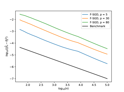
(a) $\bm{X}$ follows data generating process (a)

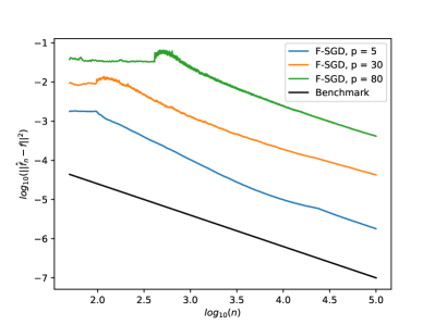
(b) $\bm{X}$ follows data generating process (b)

Figure 1: $\log_{10}\|\widehat{f}_{n}-f\|^{2}$ against $\log_{10}n$. The benchmark (black line) has slope $-2s/(2s+1)=-4/5$, which represents the minimax optimal rate. Each curve is calculated as the average of 20 repetitions. (a) $\bm{X}$ follows data generating process (a). (b) $\bm{X}$ follows data generating process (b).

Growing $p$.

In the context of growing $p$, we continue to utilize the regression function (5.1). We generate $\bm{X}$ from a uniform distribution over $[0,1]^{p}$ and $\varepsilon$ from a uniform distribution over $[-0.02,0.02]$. We select parameters according to Theorem 4.1. We set $A_{2}=5A_{1}$, $A_{1}=1$, and $B=0.5$ across all three cases corresponding to $p=5$, $30$, and $80$.

Figure 2(a) shows the convergence rate in terms of the sample size $n$. The convergence exhibits three distinct behaviors, each corresponding to the three stages of training. In the first stage, the MSE remains unchanged due to the absence of updates to $\widehat{f}_{i}$. This is followed by a transient phase, where moderate learning occurs, marking the second stage. Ultimately, in the third stage, the MSE attains minimax optimal convergence with respect to $n$. Figure 2(b) provides the convergence rate in terms of the dimension $p$. We select $p$ from the range $\{29,32,35,\dots,71\}$ and evaluate the MSE at $n=10^{5}$. It is seen that the MSE convergence is close to minimax optimal in terms of $p$.

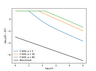
(a) Convergence rate in terms of $n$

(b) Convergence rate in terms of $p$

Figure 2: (a) $\log_{10}\|\widehat{f}_{n}-f\|^{2}$ against $\log_{10}n$. The benchmark (black line) has slope $-2s/(2s+1)=-4/5$, which represents the minimax optimal rate in terms of $n$. (b) $\log_{10}\|\widehat{f}_{n}-f\|^{2}$ against $\log_{10}p$ when $n=10^{5}$. The benchmark (black line) has slope 1, which represents the minimax optimal rate in terms of $p$. Each curve is calculated as the average of 20 repetitions.

5.2 F-SGD vs. Sieve-SGD for Univariate Models on Simulated Data

In this section, we evaluate the performance F-SGD in comparison to Sieve-SGD (Zhang and Simon, 2022) when $p=1$. The parameters provided by Zhang and Simon (2022) are specifically tailored for the case when $f\in\widetilde{W}_{p}(s,Q)$, as defined in (4.2). Therefore, we likewise assume $f$ belongs to $\widetilde{W}_{p}(s,Q)$. It is worth noting that Zhang and Simon (2022) included two other methods: kernel ridge regression (KRR) (Wainwright, 2019) and kernel SGD (Dieuleveut and Bach, 2016). The results indicated that Sieve-SGD exhibited comparable statistical performance but outperformed the other methods in terms of computational efficiency. In this section, we focus on comparing F-SGD and Sieve-SGD, but we do not include KRR and kernel SGD in our analysis. As elaborated in Section 4.2.2, F-SGD exhibits a time complexity of $\Theta\big{(}n^{1+1/(2s+1)}\big{)}$, leading us to anticipate that it will also provide enhanced computational efficiency.

We consider the regression function $f(x)=B_{4}(x)=x^{4}-2x^{3}+x^{2}-1/30$, which is the fourth Bernoulli polynomial, and we utilize the trigonometric basis. The smoothness parameter is $s=2$. Hence, $f$ belongs to Sobolev ellipsoid $W(2,Q)$ for some constant $Q$. We consider two different scenarios regarding the distribution of $X$: (a) $X$ has an uniform distribution over $[0,1]$, and (b) $X$ has an uniform distribution over $[0.25,0.75]$. It is worth mentioning that while the trigonometric basis functions are orthonormal with respect to the Lebesgue measure in scenario (a), they are not orthonormal in scenario (b). Additionally, we apply two different noise levels in these scenarios: In scenario (a), we use small noise, where $\varepsilon$ follows a uniform distribution over $[-0.02,0.02]$. In scenario (b), we use large noise, where $\varepsilon$ follows a uniform distribution over $[-0.2,0.2]$. This setup precisely mirrors the conditions presented in Example 1 of the simulation study in Zhang and Simon (2022).

In the case of F-SGD, for scenario (a), we set $\gamma_{i}=3/i$ and $J_{i}=\lfloor i^{1/(2s+1)}\rfloor=\lfloor i^{0.2}\rfloor$. In scenario (b), we set $\gamma_{i}=3/i$ and $J_{i}=\lfloor 0.8i^{1/(2s+1)}\rfloor=\lfloor 0.8i^{0.2}\rfloor$. As for Sieve-SGD, we adopt the same parameters as presented in Zhang and Simon (2022). Specifically, we use $\gamma_{i}=3/i$ and set $J_{n}=n^{0.21}$. Additionally, we choose $t_{i}=j^{-2s}=j^{-4}$, which corresponds to the oracle component-specific learning rate (Theorem 6.1 in Zhang and Simon (2022)).

Figure 3 provides empirical evidence that F-SGD converges at the minimax optimal rate and exhibits performance closely resembling Sieve-SGD when equipped with an appropriately chosen component-specific learning rate.

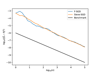
(a) Uniform distribution over 0 to 1

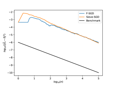
(b) Uniform distribution over 0.25 to 0.75

Figure 3: $\log_{10}\|\widehat{f}_{n}-f\|^{2}$ against $\log_{10}n$. The benchmark (black line) has slope $-2s/(2s+1)=-4/5$, which represents the minimax optimal rate. Each curve is calculated as the average of 100 repetitions. (a) $X$ is uniformly distributed over [0, 1]. (b) $X$ is uniformly distributed over [0.25, 0.75].

5.3 F-SGD vs. Backfitting for Additive Models on Real-world Data

In this section, we consider two real-world data sets to demonstrate the computational advantages of F-SGD for additive models. The first data set comprises 19,735 instances of appliance energy usage in a low-energy building. In our experiments, the appliance energy usage is treated as the response variable, while the remaining 25 variables, excluding rv1 and rv2, are treated as covariates.

The second data set consists of 288,000 instances of the positions and absorbed power outputs of wave energy converters in four real wave scenarios from the southern coast of Australia. We use the total power output as the response variable and all other 48 variables as the covariates. We substitute any missing covariate data with the (respective) average values of the observed covariate data.

For each data set, we randomly select $10\%$ of the data as the test set. From the remaining $90\%$, we further randomly allocate portions of $1\%,5\%,10\%,20\%,\dots,90\%$ as the training set. We compare the runtime (measured in seconds) of fitting F-SGD and the backfitting algorithm. In the case of F-SGD, we apply the parameter selections as outlined in Theorem 4.5 for a fixed $p$. Specifically, we set $A=2$, $B=0.4$, and $s=1$. For backfitting, we use the LinearGAM function from the pyGAM package (Servén and Brummitt, 2018) in Python, with cubic smoothing splines as the smoothers. All other parameters within the LinearGAM function are set to their default values. Our experiments were carried out on a laptop equipped with an Intel(R) Core(TM) i7-9750H CPU at 2.60 GHz and bolstered by 32GB of RAM. To ensure a fair comparison between these two iterative schemes, we have opted not to employ cross-validation. Figure 4 shows the runtime for the two data sets. It is observed that F-SGD consistently runs faster than backfitting. It is also noteworthy to mention that, while not illustrated in figures, the runtime difference between F-SGD and the backfitting algorithm becomes more pronounced as we include a great number of covariates in each data set.

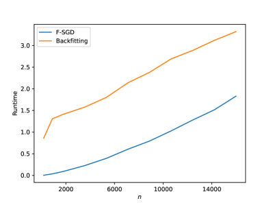
(a) Runtime for the first data set

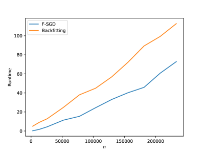
(b) Runtime for the second data set

Figure 4: Runtime measured in seconds for the data sets.

6 Discussion and Conclusion

This paper introduced a novel estimator based on SGD for learning additive nonparametric models. We demonstrated its optimal theoretical performance, favorable computational complexity, and minimal memory storage requirements under some simple conditions on the data generating process. In this section, we briefly discuss some potential future extensions.

6.1 F-SGD with Lepski’s Method

A significant advantage of F-SGD lies in the fact that the global learning rate $\gamma_{i}$ can be chosen to be independent of $s$, namely, $\gamma_{i}=\Theta(1/i)$ in the case of a fixed $p$ (see Theorem 4.5). Because of this selection, the sole dependence on $s$ is through $J_{i}$, which enables us to develop an online version of Lepski’s method.

Lepski’s method is widely used in adaptive nonparametric estimation when the smoothness parameter is unknown (Lepskii, 1991). In the classical batch setting, it achieves a rate slower than the nonadaptive minimax rate by only a logarithmic factor. At each iteration step, let $s_{i,a},s_{i,b}\in\mathcal{S}_{i}=\{s_{0},s_{0}+1/\log i,s_{0}+2/\log i,\dots,s_{1}\}$ and define $J_{i,a}=\lfloor Bi^{\frac{1}{2s_{i,a}+1}}\rfloor$ and $J_{i,b}=\lfloor Bi^{\frac{1}{2s_{i,b}+1}}\rfloor$ for some constant $B$. We then introduce $\widehat{f}_{i}^{J_{i,l}}$, where $l\in\{a,b\}$, as:

$$\widehat{f}_{i}^{J_{i,l}}(\bm{X})=\widehat{f}_{i-1}(\bm{X})+\gamma_{i}\left(Y_{i}-\widehat{f}_{i-1}\left(\bm{X}_{i}\right)\right)\left(1+\sum_{k=1}^{p}\sum_{j=1}^{J_{i,l}}\psi_{jk}\left(X_{i}^{(k)}\right)\psi_{jk}\left(\bm{X}\right)\right).$$ (6.1)

To adaptively select the smoothing parameter, we adopt the core idea of Lepski’s method at the current update. That is, we select the largest $s_{i,a}\in\mathcal{S}_{i}$ that satisfies the following inequality for all $s_{i,b}<s_{i,a}$, where $s_{i,b}\in\mathcal{S}_{i}$:

$$\left\|\widehat{f}_{i}^{J_{i,b}}-\widehat{f}_{i}^{J_{i,a}}\right\|^{2}\leq\left(\frac{i}{\log i}\right)^{-\frac{2s_{i,b}}{2s_{i,b}+1}}.$$ (6.2)

Since $p_{\bm{X}}(\bm{x})\leq C_{2}$, as per Assumption 2, we have

$$\left\|\widehat{f}_{i}^{J_{i,b}}-\widehat{f}_{i}^{J_{i,a}}\right\|^{2}\leq C_{2}\gamma_{i}^{2}\left(Y_{i}-\widehat{f}_{i-1}\left(X_{i}\right)\right)^{2}\sum_{k=1}^{p}\sum_{j=J_{i,a}+1}^{J_{i,b}}\psi_{jk}^{2}\left(X_{i}^{(k)}\right).$$

If we set $\gamma_{i}=A/i$ and absorb $C_{2}$ into $A$, we can simplify (6.2) and select the smoothing parameter by identifying the largest $s_{i,a}\in\mathcal{S}_{i}$ such that, for all $s_{i,b}<s_{i,a}$ where $s_{i,b}\in\mathcal{S}_{i}$, the following condition holds:

$$\gamma_{i}^{2}\left(Y_{i}-\widehat{f}_{i-1}\left(X_{i}\right)\right)^{2}\sum_{k=1}^{p}\sum_{j=J_{i,a}+1}^{J_{i,b}}\psi_{jk}^{2}\left(X_{i}^{(k)}\right)\leq\left(\frac{i}{\log i}\right)^{-\frac{2s_{i,b}}{2s_{i,b}+1}}.$$ (6.3)

We summarize the procedure in Algorithm 1.

For $i=1$ to $n$:

 Set $\gamma_{i}=A/i$ and $J_{i,l}=\lfloor Bi^{\frac{1}{2s_{i,l}+1}}\rfloor$ where $l\in\{a,b\}$ for some appropriate constants $A$ and $B$.

 Select the largest $s_{i,a}\in\mathcal{S}_{i}$ such that, for all $s_{i,b}<s_{i,a}$ where $s_{i,b}\in\mathcal{S}_{i}$, the condition (6.3) holds.

 Update $\widehat{f}_{i}$ according to (6.1) with $k=a$.

Algorithm 1 F-SGD with Lepski’s method

The theoretical investigation of F-SGD with Lepski’s method is beyond the scope of this paper, though we undertake a numerical study in the next section to highlight its potential. The results indicate that F-SGD with Lepski’s method exhibits favorable performance.

6.1.1 Simulations for F-SGD with Lepski’s Method

In this section, we present some numerical results for F-SGD with Lepski’s method. We again consider the function $f(x)=B_{4}(x)=x^{4}-2x^{3}+x^{2}-1/30$ and use the trigonometric basis. In contrast to previous sections, here we assume the smoothness parameter $s$ is unknown, but that it lies within the range $[s_{0},s_{1}]$ where $s_{0}=0.5$ and $s_{1}=8$. Similar to the simulation example in Section 5.2, the covariate $X$ is generated from two different distributions: (a) $X$ has a uniform distribution over $[0,1]$, and (b) $X$ has a uniform distribution over $[0.25,0.75]$. Also, we apply two different noise levels in these scenarios: In scenario (a), we use small noise, where $\varepsilon$ follows a uniform distribution over $[-0.02,0.02]$. In scenario (b), we use large noise, where $\varepsilon$ follows a uniform distribution over $[-0.2,0.2]$.

We use F-SGD with Lepski’s method (Algorithm 1) to update $\widehat{f}_{i}$. For scenario (a), we set $A=B=3$, and for scenario (b), we set $A=4$ and $B=2$. Figure 5 illustrates that even without knowing $s$ a priori, F-SGD with Lepski’s method can still achieve near minimax optimal convergence.

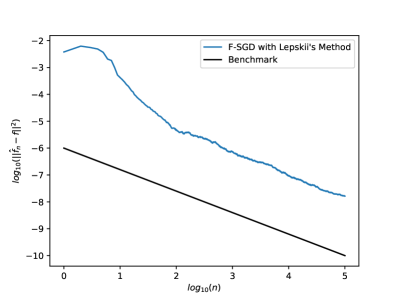
(a) Uniform distribution over 0 to 1

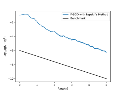
(b) Uniform distribution over 0.25 to 0.75

Figure 5: $\log_{10}\|\widehat{f}_{n}-f\|^{2}$ against $\log_{10}n$, where $\widehat{f}_{n}$ is the F-SGD with Lepski’s method. The benchmark (orange line) has slope $-2s/(2s+1)=-4/5$, which represents the optimal rate. Each curve is calculated as the average of 30 repetitions. (a) $X$ is uniformly distributed over [0, 1]. (b) $X$ is uniformly distributed over [0.25, 0.75].

6.2 General Convex Loss Functions

Suppose we aim to minimize

$$\min_{f\in\mathcal{F}_{p}}\mathbb{E}[\ell(Y,f(\bm{X}))],$$

where the loss function $\ell(u,v)$ is convex with respect to $v$ for any $u$. Following the same principle as F-SGD (3.2), we can update $\widehat{f}_{i}$ as follows:

$$\widehat{f}_{i}(\bm{X})=\widehat{f}_{i-1}(\bm{X})-\gamma_{i}\frac{\partial\ell(u,v)}{\partial v}|_{u=Y_{i},\;v=\widehat{f}_{i-1}(\bm{X})}\left(1+\sum_{k=1}^{p}\sum_{j=1}^{J_{i}}\psi_{jk}\left(X_{i}^{(k)}\right)\psi_{jk}\left(\bm{X}\right)\right).$$

Exploring the selection of parameters and characterizing the theoretical performance of this estimator are interesting directions for future research. Due to its simplicity, extensions based on our approach may be more amenable to theoretical analysis compared to, for example, Sieve-SGD (Zhang and Simon, 2022).

Appendix

In Appendix A, we provide full proofs of Theorem 4.1 and Theorem 4.5.

Appendix A Proofs

Proof of Theorem 4.1.

To prove Theorem 4.1, we first need to solve a simple recursive inequality.

Lemma A.1.

Suppose for $i\geq i_{0}$, we have $e_{i}\leq a_{i}e_{i-1}+b_{i}$ with $a_{i},b_{i},e_{i}>0$. Then for any $i\geq i_{0}$,

$$e_{i}\leq e_{i_{0}-1}\prod_{k=i_{0}}^{i}a_{k}+\sum_{k=i_{0}}^{i-1}\left(\prod_{j=k+1}^{i}a_{j}\right)b_{k}+b_{i}.$$ (A.1)

Proof.

This lemma can be proved by induction. Note that the inequality (A.1) holds when $i=i_{0}$. In addition, suppose (A.1) holds for $i$. Then,

$$e_{i+1} \leq a_{i+1}e_{i}+b_{i+1}$$

$$\leq a_{i+1}\left(e_{i_{0}-1}\prod_{k=i_{0}}^{i}a_{k}+\sum_{k=i_{0}}^{i-1}\left(\prod_{j=k+1}^{i}a_{j}\right)b_{k}+b_{i}\right)+b_{i+1}$$

$$=e_{i_{0}-1}\prod_{k=i_{0}}^{i+1}a_{k}+\sum_{k=i_{0}}^{i}\left(\prod_{j=k+1}^{i+1}a_{j}\right)b_{k}+b_{i+1}.\qed$$

Now we start to prove Theorem 4.1. To simplify the notation, at each iteration step $i$, we let $r_{i}=Y_{i}-\widehat{f}_{i-1}(\bm{X}_{i})$. Throughout the proof, the expectation operator $\mathbb{E}$ is taken with respect to all of the randomness, unless it is explicitly stated otherwise.

Using the recursive relationship (3.2) for $\widehat{f}_{i}$, we have

$$\left\|\widehat{f}_{i}-f\right\|^{2} =\left\|\widehat{f}_{i-1}-f+\gamma_{i}r_{i}\left(1+\sum_{k=1}^{p}\sum_{j=1}^{J_{i}}\psi_{jk}\left(X_{i}^{(k)}\right)\psi_{jk}\right)\right\|^{2}$$

$$=\left\|\widehat{f}_{i-1}-f\right\|^{2}+2\left\langle\widehat{f}_{i-1}-f,\gamma_{i}r_{i}\left(1+\sum_{k=1}^{p}\sum_{j=1}^{J_{i}}\psi_{jk}\left(X_{i}^{(k)}\right)\psi_{jk}\right)\right\rangle$$

$$\qquad+\gamma_{i}^{2}r_{i}^{2}\left\|1+\sum_{k=1}^{p}\sum_{j=1}^{J_{i}}\psi_{jk}\left(X_{i}^{(k)}\right)\psi_{jk}\right\|^{2}.$$ (A.2)

Next, we take the expectation of the last term in (A.2) and apply the law of iterated expectations:

$$\mathbb{E}\left[\gamma_{i}^{2}r_{i}^{2}\left\|1+\sum_{k=1}^{p}\sum_{j=1}^{J_{i}}\psi_{jk}\left(X_{i}^{(k)}\right)\psi_{jk}\right\|^{2}\right]$$

$$=~{}\mathbb{E}\left[\mathbb{E}\left[\gamma_{i}^{2}r_{i}^{2}\left\|1+\sum_{k=1}^{p}\sum_{j=1}^{J_{i}}\psi_{jk}\left(X_{i}^{(k)}\right)\psi_{jk}\right\|^{2}\Bigg{|}\bm{X}_{i},(\bm{X}_{k},Y_{k})_{k=1}^{i-1}\right]\right].$$ (A.3)

Note that $\mathbb{E}[r_{i}^{2}\mid\bm{X}_{i},(\bm{X}_{k},Y_{k})_{k=1}^{i-1}]\leq\sigma^{2}+\big{(}\widehat{f}_{i-1}(\bm{X}_{i})-f(\bm{X}_{i})\big{)}^{2}$. Also, we have the inequality

$$\left\|1+\sum_{k=1}^{p}\sum_{j=1}^{J_{i}}\psi_{jk}\left(X_{i}^{(k)}\right)\psi_{jk}\right\|^{2} =\int\left(1+\sum_{k=1}^{p}\sum_{j=1}^{J_{i}}\psi_{jk}\left(X_{i}^{(k)}\right)\psi_{jk}\left(x^{(k)}\right)\right)^{2}p_{X}(\bm{x})d\bm{x}$$

$$\leq C_{2}\int\left(1+\sum_{k=1}^{p}\sum_{j=1}^{J_{i}}\psi_{jk}\left(X_{i}^{(k)}\right)\psi_{jk}\left(x^{(k)}\right)\right)^{2}d\bm{x}$$

$$=C_{2}\left(1+\sum_{k=1}^{p}\sum_{j=1}^{J_{i}}\psi_{jk}^{2}\left(X_{i}^{(k)}\right)\right),$$ (A.4)

where for the first inequality, we use Assumption 2 which says that $p_{\bm{X}}(\bm{x})\leq C_{2}$, and for the last equality, we use the fact that $\psi_{jk}$ are centered ($\int\psi_{jk}(x)dx=0$), and for a given $k$, the basis $\{\psi_{jk}\}_{j}$ is orthonormal. Thus, putting (A.3) and (A.4) together, we have

$$\mathbb{E}\left[\gamma_{i}^{2}r_{i}^{2}\left\|1+\sum_{k=1}^{p}\sum_{j=1}^{J_{i}}\psi_{jk}\left(X_{i}^{(k)}\right)\psi_{jk}\right\|^{2}\right]$$

$$\leq~{}\mathbb{E}\left[\gamma_{i}^{2}(\sigma^{2}+(\widehat{f}_{i-1}(\bm{X}_{i})-f(\bm{X}_{i}))^{2})C_{2}\left(1+\sum_{k=1}^{p}\sum_{j=1}^{J_{i}}\psi_{jk}^{2}\left(X_{i}^{(k)}\right)\right)\right]$$

$$\leq~{}\gamma_{i}^{2}\left(\sigma^{2}+\mathbb{E}\Big{[}\left\|\widehat{f}_{i-1}-f\right\|^{2}\Big{]}\right)C_{2}\left(1+pJ_{i}M^{2}\right),$$ (A.5)

where the last inequality directly follows from the boundedness of $\psi_{jk}$. To compute the second term in (A.2), we first expand the inner product

$$\mathbb{E}\left[\left\langle\widehat{f}_{i-1}-f,\gamma_{i}r_{i}\left(1+\sum_{k=1}^{p}\sum_{j=1}^{J_{i}}\psi_{jk}\left(X_{i}^{(k)}\right)\psi_{jk}\right)\right\rangle\right]$$

$$=~{}\gamma_{i}\mathbb{E}\left[\left\langle\widehat{f}_{i-1}-f,\left(f(\bm{X}_{i})-\widehat{f}_{i-1}(\bm{X}_{i})\right)\left(1+\sum_{k=1}^{p}\sum_{j=1}^{J_{i}}\psi_{jk}\left(X_{i}^{(k)}\right)\psi_{jk}\right)\right\rangle\right]$$

$$=~{}-\gamma_{i}\Bigg{(}\mathbb{E}\left[\left|\left\langle\widehat{f}_{i-1}-f,1\right\rangle\right|^{2}\right]+\sum_{k=1}^{p}\sum_{j=1}^{J_{i}}\mathbb{E}\left[\left|\left\langle\widehat{f}_{i-1}-f,\psi_{jk}\right\rangle\right|^{2}\right]\Bigg{)},$$ (A.6)

where for the last equality we use the fact that $\widehat{f}_{i-1}$ is independent of $\bm{X}_{i}$. Let $f_{k}=\sum_{j=1}^{\infty}\theta_{f,j}^{(k)}\psi_{jk}$ where $\theta_{f,j}^{(k)}=\int f_{k}(x)\psi_{jk}(x)dx$, $f_{k,i}=\sum_{j=1}^{J_{i}}\theta_{f,j}^{(k)}\psi_{jk}$, and $\check{f}_{i}=\alpha+\sum_{k=1}^{p}f_{k,i}$. Since $\widehat{f}_{i-1}$ and $\check{f}_{i}$ belong to $\text{span}\{\psi_{0},\,\psi_{jk}:j=1,2,\dots,J_{i}\text{ and }k=1,2,\dots,p\}$ where $\psi_{0}\equiv 1$, we can write $\widehat{f}_{i-1}-\check{f}_{i}=\widehat{\alpha}_{i-1}+\sum_{k=1}^{p}\sum_{j=1}^{J_{i}}\widehat{\beta}_{i-1,j}^{(k)}\psi_{jk}$, where

$$\widehat{\beta}_{i-1,j}^{(k)}=\int\left(\widehat{f}_{i-1}(\bm{x})-\check{f}_{i}(\bm{x})\right)\psi_{jk}\left(x^{(k)}\right)d\bm{x},\qquad\widehat{\alpha}_{i-1}=\int\left(\widehat{f}_{i-1}(\bm{x})-\check{f}_{i}(\bm{x})\right)d\bm{x}.$$

Hence, we have

$$\left|\mathbb{E}\left[\left\langle\widehat{f}_{i-1}-f,\widehat{f}_{i-1}-\check{f}_{i}\right\rangle\right]\right|^{2}$$

$$=~{}\bigg{(}\mathbb{E}\left[\int\left(\widehat{f}_{i-1}(\bm{x})-f(\bm{x})\right)\widehat{\alpha}_{i-1}p_{X}(\bm{x})d\bm{x}\right]$$

$$\qquad+\sum_{k=1}^{p}\sum_{j=1}^{J_{i}}\mathbb{E}\left[\int\left(\widehat{f}_{i-1}(\bm{x})-f(\bm{x})\right)\widehat{\beta}_{i-1,j}^{(k)}\psi_{jk}\left(x^{(k)}\right)p_{X}(\bm{x})d\bm{x}\right]\bigg{)}^{2}.$$

Using the Cauchy-Schwarz inequality, we know

$$\left|\mathbb{E}\left[\left\langle\widehat{f}_{i-1}-f,\widehat{f}_{i-1}-\check{f}_{i}\right\rangle\right]\right|^{2}$$

$$\leq\Bigg{(}\mathbb{E}\left[\left(\int\left(\widehat{f}_{i-1}(\bm{x})-f(\bm{x})\right)p_{X}(\bm{x})d\bm{x}\right)^{2}\right]$$

$$\qquad+\sum_{k=1}^{p}\sum_{j=1}^{J_{i}}\mathbb{E}\left[\left(\int\left(\widehat{f}_{i-1}(\bm{x})-f(\bm{x})\right)\psi_{jk}\left(x^{(k)}\right)p_{X}(\bm{x})d\bm{x}\right)^{2}\right]\Bigg{)}\mathbb{E}\Bigg{[}\widehat{\alpha}_{i-1}^{2}+\sum_{k=1}^{p}\sum_{j=1}^{J_{i}}\Big{(}\widehat{\beta}_{i-1,j}^{(k)}\Big{)}^{2}\Bigg{]}$$

$$=~{}\Bigg{(}\mathbb{E}\left[\left|\left\langle\widehat{f}_{i-1}-f,1\right\rangle\right|^{2}\right]+\sum_{k=1}^{p}\sum_{j=1}^{J_{i}}\mathbb{E}\left[\left|\left\langle\widehat{f}_{i-1}-f,\psi_{jk}\right\rangle\right|^{2}\right]\Bigg{)}\mathbb{E}\Bigg{[}\widehat{\alpha}_{i-1}^{2}+\sum_{k=1}^{p}\sum_{j=1}^{J_{i}}\Big{(}\widehat{\beta}_{i-1,j}^{(k)}\Big{)}^{2}\Bigg{]}.$$ (A.7)

Furthermore, by Assumption 2 which says that $p_{\bm{X}}(\bm{x})\geq C_{1}$, we have

$$\mathbb{E}\Bigg{[}\widehat{\alpha}_{i-1}^{2}+\sum_{k=1}^{p}\sum_{j=1}^{J_{i}}\Big{(}\widehat{\beta}_{i-1,j}^{(k)}\Big{)}^{2}\Bigg{]}$$

$$\leq~{}\mathbb{E}\Bigg{[}\int\left(\widehat{\alpha}_{i-1}+\sum_{k=1}^{p}\sum_{j=1}^{J_{i}}\widehat{\beta}_{i-1,j}^{(k)}\psi_{jk}\left(x^{(k)}\right)-\sum_{k=1}^{p}\sum_{j=J_{i}+1}^{\infty}\theta_{f,j}^{(k)}\psi_{jk}\left(x^{(k)}\right)\right)^{2}d\bm{x}\Bigg{]}$$

$$\leq~{}\frac{1}{C_{1}}\mathbb{E}\Bigg{[}\int\left(\widehat{\alpha}_{i-1}+\sum_{k=1}^{p}\sum_{j=1}^{J_{i}}\widehat{\beta}_{i-1,j}^{(k)}\psi_{jk}\left(x^{(k)}\right)-\sum_{k=1}^{p}\sum_{j=J_{i}+1}^{\infty}\theta_{f,j}^{(k)}\psi_{jk}\left(x^{(k)}\right)\right)^{2}p_{X}(\bm{x})d\bm{x}\Bigg{]}$$

$$=~{}\frac{1}{C_{1}}\mathbb{E}\Big{[}\left\|\widehat{f}_{i-1}-f\right\|^{2}\Big{]}.$$ (A.8)

In addition, note that

$$\left|\mathbb{E}\left[\left\langle\widehat{f}_{i-1}-f,\widehat{f}_{i-1}-\check{f}_{i}\right\rangle\right]\right|^{2}$$

$$=~{}\left|\mathbb{E}\left[\left\|\widehat{f}_{i-1}-f\right\|^{2}\right]+\mathbb{E}\left[\left\langle\widehat{f}_{i-1}-f,f-\check{f}_{i}\right\rangle\right]\right|^{2}$$

$$\geq~{}\left(\mathbb{E}\left[\left\|\widehat{f}_{i-1}-f\right\|^{2}\right]\right)^{2}+2\left(\mathbb{E}\left[\left\|\widehat{f}_{i-1}-f\right\|^{2}\right]\right)\left(\mathbb{E}\left[\left\langle\widehat{f}_{i-1}-f,f-\check{f}_{i}\right\rangle\right]\right).$$ (A.9)

By the AM-GM inequality, we know

$$2\mathbb{E}\left[\left\langle\widehat{f}_{i-1}-f,f-\check{f}_{i}\right\rangle\right]\geq-\frac{1}{2}\mathbb{E}\left[\left\|\widehat{f}_{i-1}-f\right\|^{2}\right]-2\left\|f-\check{f}_{i}\right\|^{2}.$$

Hence, continuing from (A.9), we obtain

$$\left|\mathbb{E}\left[\left\langle\widehat{f}_{i-1}-f,\widehat{f}_{i-1}-\check{f}_{i}\right\rangle\right]\right|^{2}$$

$$\geq~{}\left(\mathbb{E}\left[\left\|\widehat{f}_{i-1}-f\right\|^{2}\right]\right)^{2}-\left(\mathbb{E}\left[\left\|\widehat{f}_{i-1}-f\right\|^{2}\right]\right)\left(\frac{1}{2}\mathbb{E}\left[\left\|\widehat{f}_{i-1}-f\right\|^{2}\right]+2\left\|f-\check{f}_{i}\right\|^{2}\right)$$

$$=~{}\frac{1}{2}\left(\mathbb{E}\left[\left\|\widehat{f}_{i-1}-f\right\|^{2}\right]\right)^{2}-2\left(\mathbb{E}\left[\left\|\widehat{f}_{i-1}-f\right\|^{2}\right]\right)\left(\left\|f-\check{f}_{i}\right\|^{2}\right).$$ (A.10)

Moreover, let $g=\tau+\sum_{k=1}^{p}g_{k}$ with $g_{k}\in\mathcal{H}_{1}(s)$ for any $k=1,2,\dots,p$ and any $\tau\in\mathbb{R}$. Suppose $g_{k}=\sum_{j=1}^{\infty}\theta_{g,j}^{(k)}\psi_{jk}$. Define $g_{k,i}=\sum_{j=1}^{J_{i}}\theta_{g,j}^{(k)}\psi_{jk}$ and $\check{g}_{i}=\tau+\sum_{k=1}^{p}g_{k,i}$. Then, we have

$$\left\|f-\check{f}_{i}\right\|^{2}\leq\left(\left\|f-g\right\|+\left\|g-\check{g}_{i}\right\|+\left\|\check{g}_{i}-\check{f}_{i}\right\|\right)^{2}.$$ (A.11)

Note that

$$\left\|\check{g}_{i}-\check{f}_{i}\right\|^{2} \leq C_{2}\int(\check{g}_{i}(\bm{x})-\check{f}_{i}(\bm{x}))^{2}d\bm{x}$$

$$\leq C_{2}\int(g(\bm{x})-f(\bm{x}))^{2}d\bm{x}$$

$$\leq\frac{C_{2}}{C_{1}}\left\|g-f\right\|^{2},$$ (A.12)

where we use Assumption 2 again, i.e., $C_{1}\leq p_{\bm{X}}(\bm{x})\leq C_{2}$. Also, we know

$$\left\|g-\check{g}_{i}\right\|^{2} =\int\left(\sum_{k=1}^{p}\sum_{j=J_{i}+1}^{\infty}\theta_{g,j}^{(k)}\psi_{jk}\left(x^{(k)}\right)\right)^{2}p_{X}(\bm{x})d\bm{x}$$

$$\leq C_{2}\int\left(\sum_{k=1}^{p}\sum_{j=J_{i}+1}^{\infty}\theta_{g,j}^{(k)}\psi_{jk}\left(x^{(k)}\right)\right)^{2}d\bm{x}$$

$$=C_{2}\sum_{k=1}^{p}\sum_{j=J_{i}+1}^{\infty}\left(\theta_{g,j}^{(k)}\right)^{2}$$

$$\leq C_{2}\sum_{k=1}^{p}\frac{1}{J_{i}^{2s}}\sum_{j=J_{i}+1}^{\infty}\left(\theta_{g,j}^{(k)}\right)^{2}j^{2s}\leq\frac{C_{2}\sum_{k=1}^{p}\|g_{k}\|_{s}^{2}}{J_{i}^{2s}}.$$ (A.13)

Continuing from (A.11), we utilize (A.12) and (A.13), and obtain

$$\left\|f-\check{f}_{i}\right\|^{2} \leq 2\left(\|f-g\|+\|\check{g}_{i}-\check{f}_{i}\|\right)^{2}+2\|g-\check{g}_{i}\|^{2}$$

$$\leq 2\left(1+\sqrt{\frac{C_{2}}{C_{1}}}\right)^{2}\left\|g-f\right\|^{2}+\frac{2C_{2}\sum_{k=1}^{p}\|g_{k}\|_{s}^{2}}{J_{i}^{2s}}.$$ (A.14)

Hence, combining inequalities (A.6)-(A.10) and (A.14), we know

$$\mathbb{E}\left[\left\langle\widehat{f}_{i-1}-f,\gamma_{i}r_{i}\left(1+\sum_{k=1}^{p}\sum_{j=1}^{J_{i}}\psi_{jk}\left(X_{i}^{(k)}\right)\psi_{jk}\right)\right\rangle\right]$$

$$\leq~{}-\frac{\gamma_{i}}{2}C_{1}\mathbb{E}\left[\left\|\widehat{f}_{i}-f\right\|^{2}\right]+4\gamma_{i}C_{1}\left(1+\sqrt{\frac{C_{2}}{C_{1}}}\right)^{2}\left\|g-f\right\|^{2}+\gamma_{i}\frac{4C_{1}C_{2}\sum_{k=1}^{p}\|g_{k}\|_{s}^{2}}{J_{i}^{2s}}.$$ (A.15)

To simplify the notation, we let $e_{i}=\mathbb{E}\big{[}\|\widehat{f}_{i}-f\|^{2}\big{]}$. By (A.2), (A.5), and (A.15), we have for any $i\geq 1$,

$$e_{i} \leq\left(1-C_{1}\gamma_{i}+C_{2}\left(pM^{2}J_{i}+1\right)\gamma_{i}^{2}\right)e_{i-1}$$

$$\qquad+C_{2}\sigma^{2}(pM^{2}J_{i}+1)\gamma_{i}^{2}+8\gamma_{i}C_{1}C_{2}\frac{\sum_{k=1}^{p}\|g_{k}\|_{s}^{2}}{J_{i}^{2s}}+8\gamma_{i}C_{1}\left(1+\sqrt{\frac{C_{2}}{C_{1}}}\right)^{2}\left\|g-f\right\|^{2}$$

$$\leq\left(1-C_{1}\gamma_{i}+2C_{2}pM^{2}J_{i}\gamma_{i}^{2}\right)e_{i-1}$$

$$\qquad+2C_{2}\sigma^{2}pM^{2}J_{i}\gamma_{i}^{2}+8\gamma_{i}C_{1}C_{2}\frac{\sum_{k=1}^{p}\|g_{k}\|_{s}^{2}}{J_{i}^{2s}}+8\gamma_{i}C_{1}\left(1+\sqrt{\frac{C_{2}}{C_{1}}}\right)^{2}\left\|g-f\right\|^{2},$$ (A.16)

since $p,M,J_{i}\geq 1$. When $1\leq i\leq p/B$, note that we take $\gamma_{i}=J_{i}=0$ and hence $\widehat{f}_{i}=0$. When $p/B<i\leq p^{1+1/2s}$, since $Bi/p>1$, we know $Bi/p\leq J_{i}=\lceil Bi/p\rceil\leq 2Bi/p$. Then, continuing from (A.16), we have

$$e_{i} \leq\left(1-\frac{C_{1}A_{1}}{i}+\frac{4C_{2}BM^{2}A_{1}^{2}}{i}\right)e_{i-1}+\frac{\widetilde{C}_{1}\left\|g-f\right\|^{2}+\widetilde{C}_{2}\sigma^{2}}{i}+\frac{\widetilde{C}_{3}p^{1+2s}}{i^{1+2s}}\frac{\sum_{k=1}^{p}\|g_{k}\|_{s}^{2}}{p},$$ (A.17)

where $\widetilde{C}_{1}=8A_{1}C_{1}(1+\sqrt{C_{2}/C_{1}})^{2}$, $\widetilde{C}_{2}=4C_{2}BM^{2}A_{1}^{2}$, and $\widetilde{C}_{3}=8A_{1}C_{1}C_{2}/B^{2s}$. Note that $A_{1}\geq 2(2s+1)/C_{1}$ and $B\leq(2s+1)/(4C_{2}M^{2}A_{1}^{2})$. Continuing from (A.17), we have for any $p/B<i\leq p^{1+1/2s}$,

$$e_{i} \leq\left(1-\frac{2s+1}{i}\right)e_{i-1}+\frac{\widetilde{C}_{1}\left\|g-f\right\|^{2}+\widetilde{C}_{2}\sigma^{2}}{i}+\frac{\widetilde{C}_{3}p^{1+2s}}{i^{1+2s}}\frac{\sum_{k=1}^{p}\|g_{k}\|_{s}^{2}}{p}$$

$$\leq\left(1-\frac{1}{i}\right)^{2s+1}e_{i-1}+\frac{\widetilde{C}_{1}\left\|g-f\right\|^{2}+\widetilde{C}_{2}\sigma^{2}}{i}+\frac{\widetilde{C}_{3}p^{1+2s}}{i^{1+2s}}\frac{\sum_{k=1}^{p}\|g_{k}\|_{s}^{2}}{p}$$

$$\leq\left(1-\frac{1}{i}\right)^{2s+1}e_{i-1}+\frac{p^{1+2s}}{i^{1+2s}}\left(\widetilde{C}_{3}\frac{\sum_{k=1}^{p}\|g_{k}\|_{s}^{2}}{p}+\widetilde{C}_{1}\left\|g-f\right\|^{2}+\widetilde{C}_{2}\sigma^{2}\right),$$ (A.18)

where we use Bernoulli’s inequality, i.e., $(1+z)^{r}\geq 1+zr$ for all $r\geq 1$ and $z\geq-1$, for the second inequality. Note that

$$\prod_{j=k+1}^{i}\left(1-\frac{1}{j}\right)^{2s+1}=\bigg{(}\frac{k}{i}\bigg{)}^{2s+1}.$$

We now invoke Lemma A.1, taking $i_{0}=\lfloor p/B\rfloor+1$ and $i=\lfloor p^{1+1/2s}\rfloor$ in (A.1), to obtain

$$e_{\lfloor p^{1+1/2s}\rfloor} \leq\frac{1}{(2B)^{2s+1}}\frac{e_{\lfloor p/B_{1}\rfloor}}{p^{(2s+1)/2s}}+\widetilde{C}_{3}\frac{\sum_{k=1}^{p}\|g_{k}\|_{s}^{2}}{p}+\widetilde{C}_{1}\left\|g-f\right\|^{2}+\widetilde{C}_{2}\sigma^{2}$$

$$\leq\widetilde{C}_{3}\frac{\sum_{k=1}^{p}\|g_{k}\|_{s}^{2}}{p}+\widetilde{C}_{1}\left\|g-f\right\|^{2}+\frac{1}{(2B)^{2s+1}}\frac{\|f\|^{2}}{p}+\widetilde{C}_{2}\sigma^{2},$$ (A.19)

where in the last equality, we use the fact that $e_{\lfloor p/B\rfloor}=\|f\|^{2}$.

When $i>p^{1+1/2s}$, according to (A.16) and the fact that $Bi^{1/(2s+1)}\leq J_{i}\leq 2Bi^{1/(2s+1)}$, we have

$$e_{i} \leq\left(1-\frac{C_{1}A_{2}}{i}+\frac{4pC_{2}BM^{2}A_{2}^{2}}{i^{1+\frac{2s}{2s+1}}}\right)e_{i-1}+\frac{\widetilde{C}_{4}\left(p\sigma^{2}+\sum_{k=1}^{p}\|g_{k}\|_{s}^{2}\right)}{i^{1+\frac{2s}{2s+1}}}+\frac{\widetilde{C}_{5}\left\|g-f\right\|^{2}}{i},$$ (A.20)

where $\widetilde{C}_{4}=\max\{4C_{2}BM^{2}A_{2}^{2},8A_{2}C_{1}C_{2}/B^{2s}\}$ and $\widetilde{C}_{5}=8A_{2}C_{1}\big{(}1+\sqrt{C_{2}/C_{1}}\big{)}^{2}$. Note that when $A_{2}\geq 2/C_{1}$ and $B\leq 1/(4C_{2}M^{2}A_{2}^{2})$, continuing from (A.20), we have for any $i>p^{1+1/2s}$,

$$e_{i}\leq\Big{(}1-\frac{1}{i}\Big{)}e_{i-1}+\frac{\widetilde{C}_{4}\left(p\sigma^{2}+\sum_{k=1}^{p}\|g_{k}\|_{s}^{2}\right)}{i^{1+\frac{2s}{2s+1}}}+\frac{\widetilde{C}_{5}\left\|g-f\right\|^{2}}{i}.$$

We use Lemma A.1 again, this time taking $i_{0}=\lfloor p^{1+1/2s}\rfloor+1$ and $i=n$. We obtain

$$e_{n} \leq e_{\lfloor p^{1+1/2s}\rfloor}\frac{p^{1+1/2s}}{n}+\frac{n-p^{1+1/2s}-1}{n}\widetilde{C}_{5}\left\|g-f\right\|^{2}+\sum_{i=\lfloor p^{1+1/2s}\rfloor+1}^{n-1}\frac{\widetilde{C}_{4}\left(p\sigma^{2}+\sum_{k=1}^{p}\|g_{k}\|_{s}^{2}\right)}{ni^{\frac{2s}{2s+1}}}$$

$$\leq pn^{-\frac{2s}{2s+1}}C_{0}^{-\frac{1}{2s+1}}\left(\widetilde{C}_{3}\frac{\sum_{k=1}^{p}\|g_{k}\|_{s}^{2}}{p}+\widetilde{C}_{1}\left\|g-f\right\|^{2}+\frac{1}{(2B)^{2s+1}}\frac{\|f\|^{2}}{p}+\widetilde{C}_{2}\sigma^{2}\right)$$

$$\qquad+\widetilde{C}_{5}\left\|g-f\right\|^{2}+\widetilde{C}_{4}\left(p\sigma^{2}+\sum_{k=1}^{p}\|g_{k}\|_{s}^{2}\right)(2s+1)n^{-\frac{2s}{2s+1}},$$ (A.21)

where for the last inequality we use (A.19) and the fact that $\frac{1}{n}\sum_{i=1}^{n}i^{-\frac{2s}{2s+1}}\leq(2s+1)n^{-\frac{2s}{2s+1}}$. The inequality (A.21) holds for $g=\tau+\sum_{k=1}^{p}g_{k}$ with any $g_{k}\in\mathcal{H}_{1}(s)$ for $k=1,2,\dots,p$ and any $\tau\in\mathbb{R}$.

So we conclude that there exists a universal constant $C$ such that

$$\mathbb{E}\left[\|\widehat{f}_{n}-f\|^{2}\right]\leq C\inf_{g\in\mathcal{H}_{p}(s)}\Bigg{\{}\|g-f\|^{2}+\left(p\sigma^{2}+\|f\|^{2}+\sum_{k=1}^{p}\|g_{k}\|^{2}_{s}\right)n^{-\frac{2s}{2s+1}}\Bigg{\}}.$$

Here $C$ depends on $C_{1},C_{2},M$, and $s$. ∎

Proof of Theorem 4.5.

The proof of Theorem 4.5 follows a similar argument as that of Theorem 4.1. For brevity, we only highlight the main differences here.

When $p$ is fixed, it follows that $\|f\|^{2}$ is a constant, if each $\|f_{k}\|^{2}$ is constant. When $i<1/B^{2s+1}$, we note that $J_{i}=0$. Employing a reasoning analogous to that in Theorem 4.1, it holds that

$$e_{i} \leq(1+\gamma_{i}^{2})e_{i-1}+\gamma_{i}^{2}\sigma^{2}-2\gamma_{i}\mathbb{E}\bigg{[}\left|\left\langle\widehat{f}_{i-1}-f,1\right\rangle\right|^{2}\bigg{]}$$

$$\leq(1+\gamma_{i}^{2})e_{i-1}+\gamma_{i}^{2}\sigma^{2}.$$

Note that we have

$$\prod_{j=k+1}^{i}\Bigg{(}1+\frac{A^{2}}{j^{2}}\Bigg{)} =\exp\Bigg{\{}\sum_{j=k+1}^{i}\log(1+\frac{A^{2}}{j^{2}})\Bigg{\}}$$

$$\leq\exp\Bigg{\{}\sum_{j=k+1}^{i}\frac{A^{2}}{j^{2}}\Bigg{\}}$$

$$\leq\exp\Bigg{\{}\sum_{j=k+1}^{i}A^{2}\left(\frac{1}{j-1}-\frac{1}{j}\right)\Bigg{\}}\leq e^{A^{2}/k},$$

and

$$\sum_{k=1}^{\lfloor 1/B^{2s+1}\rfloor-1}\frac{1}{k^{2}}e^{A^{2}/k}\leq\int_{1}^{\lfloor 1/B^{2s+1}\rfloor}\frac{1}{x^{2}}e^{A^{2}/x}dx\leq\frac{e^{A^{2}}}{A^{2}}.$$

Thus, using Lemma A.1 by taking $i_{0}=1$ and $i=\lfloor 1/B^{2s+1}\rfloor$, we know

$$e_{\lfloor 1/B^{2s+1}\rfloor}\leq\widetilde{C}_{1}\|f\|^{2}+\widetilde{C}_{2}\sigma^{2},$$

where $\widetilde{C}_{1}=e^{1.5A^{2}}$ and $\widetilde{C}_{2}=e^{A^{2}}/A^{2}+A^{2}/\lfloor 1/B^{2s+1}\rfloor^{2}$ are two constants. When $i>\lfloor 1/B^{2s+1}\rfloor$, we know $Bi^{1/(2s+1)}/2\leq J_{i}\leq Bi^{1/(2s+1)}$. Continuing from (A.16), we have

$$e_{i} \leq\left(1-\frac{C_{1}A}{i}+\frac{2pC_{2}BM^{2}A^{2}}{i^{1+\frac{2s}{2s+1}}}\right)e_{i-1}+\frac{\widetilde{C}_{3}\left(p\sigma^{2}+\sum_{k=1}^{p}\|g_{k}\|_{s}^{2}\right)}{i^{1+\frac{2s}{2s+1}}}+\frac{\widetilde{C}_{4}\left\|g-f\right\|^{2}}{i}$$

$$\leq\left(1-\frac{1}{i}\right)e_{i-1}+\frac{\widetilde{C}_{3}\left(p\sigma^{2}+\sum_{k=1}^{p}\|g_{k}\|_{s}^{2}\right)}{i^{1+\frac{2s}{2s+1}}}+\frac{\widetilde{C}_{4}\left\|g-f\right\|^{2}}{i},$$

where $\widetilde{C}_{3}=\max\{2C_{2}BM^{2}A^{2},2^{2s+3}AC_{1}C_{2}/B^{2s}\}$ and $\widetilde{C}_{4}=8AC_{1}\big{(}1+\sqrt{C_{2}/C_{1}}\big{)}^{2}$, and $A$ and $B$ satisfy $A\geq\frac{2}{C_{1}}$ and $B\leq\frac{1}{2pC_{2}M^{2}A^{2}}$, respectively. The remainder of the proof follows the same steps as the case where $i>p^{1+1/2s}$, in the proof of Theorem 4.1. ∎

References

- Buja et al. [1989] Andreas Buja, Trevor Hastie, and Robert Tibshirani. Linear smoothers and additive models. The Annals of Statistics, 17(2):453–510, 1989. ISSN 00905364. URL http://www.jstor.org/stable/2241560.
- Chung [1954] K. L. Chung. On a Stochastic Approximation Method. The Annals of Mathematical Statistics, 25(3):463 – 483, 1954. doi: 10.1214/aoms/1177728716. URL https://doi.org/10.1214/aoms/1177728716.
- Dai et al. [2014] Bo Dai, Bo Xie, Niao He, Yingyu Liang, Anant Raj, Maria-Florina F Balcan, and Le Song. Scalable kernel methods via doubly stochastic gradients. Advances in Neural Information Processing Systems, 27, 2014.
- Dieuleveut and Bach [2016] Aymeric Dieuleveut and Francis Bach. Nonparametric stochastic approximation with large step-sizes. The Annals of Statistics, 44(4):1363–1399, 2016. ISSN 00905364. URL http://www.jstor.org/stable/43974719.
- Friedman and Stuetzle [1981] Jerome H. Friedman and Werner Stuetzle. Projection pursuit regression. Journal of the American Statistical Association, 76(376):817–823, 1981. ISSN 01621459. URL http://www.jstor.org/stable/2287576.
- Goodfellow et al. [2016] Ian Goodfellow, Yoshua Bengio, and Aaron Courville. Deep Learning. MIT Press, 2016. http://www.deeplearningbook.org.
- Györfi et al. [2002] László Györfi, Michael Kohler, Adam Krzyzak, and Harro Walk. A Distribution-Free Theory of Nonparametric Regression, volume 1. Springer, 2002.
- Hastie and Tibshirani [1990] T.J. Hastie and R.J. Tibshirani. Generalized Additive Models. Chapman & Hall/CRC Monographs on Statistics & Applied Probability. Taylor & Francis, 1990. ISBN 9780412343902. URL https://books.google.com/books?id=qa29r1Ze1coC.
- Kauermann and Opsomer [2003] Göran Kauermann and J. D. Opsomer. Local likelihood estimation in generalized additive models. Scandinavian Journal of Statistics, 30(2):317–337, 2003. ISSN 03036898, 14679469. URL http://www.jstor.org/stable/4616766.
- Koppel et al. [2019] Alec Koppel, Garrett Warnell, Ethan Stump, and Alejandro Ribeiro. Parsimonious online learning with kernels via sparse projections in function space. Journal of Machine Learning Research, 20(3):1–44, 2019. URL http://jmlr.org/papers/v20/16-585.html.
- Lepskii [1991] O. V. Lepskii. On a problem of adaptive estimation in gaussian white noise. Theory of Probability & Its Applications, 35(3):454–466, 1991. doi: 10.1137/1135065. URL https://doi.org/10.1137/1135065.
- Lu et al. [2016] Jing Lu, Steven C.H. Hoi, Jialei Wang, Peilin Zhao, and Zhi-Yong Liu. Large scale online kernel learning. Journal of Machine Learning Research, 17(47):1–43, 2016. URL http://jmlr.org/papers/v17/14-148.html.
- Mammen et al. [1999] E. Mammen, O. Linton, and J. Nielsen. The existence and asymptotic properties of a backfitting projection algorithm under weak conditions. The Annals of Statistics, 27(5):1443–1490, 1999. ISSN 00905364. URL http://www.jstor.org/stable/2674078.
- Raskutti et al. [2009] Garvesh Raskutti, Bin Yu, and Martin J Wainwright. Lower bounds on minimax rates for nonparametric regression with additive sparsity and smoothness. Advances in Neural Information Processing Systems, 22, 2009.
- Servén and Brummitt [2018] Daniel Servén and Charlie Brummitt. pygam: Generalized additive models in python. Zenodo. doi, 10, 2018.
- Stone [1985] Charles J. Stone. Additive regression and other nonparametric models. The Annals of Statistics, 13(2):689–705, 1985. ISSN 00905364. URL http://www.jstor.org/stable/2241204.
- Tarrès and Yao [2014] Pierre Tarrès and Yuan Yao. Online learning as stochastic approximation of regularization paths: Optimality and almost-sure convergence. IEEE Transactions on Information Theory, 60(9):5716–5735, 2014. doi: 10.1109/TIT.2014.2332531.
- Tsybakov [2009] Alexandre B. Tsybakov. Introduction to Nonparametric Estimation. Springer series in statistics. Springer, 2009. ISBN 978-0-387-79051-0. doi: 10.1007/B13794. URL https://doi.org/10.1007/b13794.
- Wainwright [2019] Martin J. Wainwright. High-Dimensional Statistics: A Non-Asymptotic Viewpoint. Cambridge Series in Statistical and Probabilistic Mathematics. Cambridge University Press, 2019. doi: 10.1017/9781108627771.
- Yang et al. [2023] Ying Yang, Fang Yao, and Peng Zhao. Online smooth backfitting for generalized additive models. Journal of the American Statistical Association, 0(0):1–29, 2023. doi: 10.1080/01621459.2023.2182213. URL https://doi.org/10.1080/01621459.2023.2182213.
- Ying and Pontil [2008] Yiming Ying and Massimiliano Pontil. Online gradient descent learning algorithms. Foundations of Computational Mathematics, 8:561–596, 01 2008. doi: 10.1007/s10208-006-0237-y.
- Yu et al. [2008] Kyusang Yu, Byeong U. Park, and Enno Mammen. Smooth backfitting in generalized additive models. The Annals of Statistics, 36(1):228–260, 2008. ISSN 00905364. URL http://www.jstor.org/stable/25464622.
- Zhang and Simon [2022] Tianyu Zhang and Noah Simon. A sieve stochastic gradient descent estimator for online nonparametric regression in Sobolev ellipsoids. The Annals of Statistics, 50(5):2848 – 2871, 2022. doi: 10.1214/22-AOS2212. URL https://doi.org/10.1214/22-AOS2212.