Interacting stochastic processes on sparse random graphs

Abstract.

Large ensembles of stochastically evolving interacting particles describe phenomena in diverse fields including statistical physics, neuroscience, biology, and engineering. In such systems, the infinitesimal evolution of each particle depends only on its own state (or history) and the states (or histories) of neighboring particles with respect to an underlying, possibly random, interaction graph. While these high-dimensional processes are typically too complex to be amenable to exact analysis, their dynamics are quite well understood when the interaction graph is the complete graph. In this case, classical theorems show that in the limit as the number of particles goes to infinity, the dynamics of the empirical measure and the law of a typical particle coincide and can be characterized in terms of a much more tractable dynamical system of reduced dimension called the mean-field limit. In contrast, until recently not much was known about corresponding convergence results in the complementary case when the interaction graph is sparse (i.e., with uniformly bounded average degree). This article provides a brief survey of classical work and then describes recent progress on the sparse regime that relies on a combination of techniques from random graph theory, Markov random fields, and stochastic analysis. The article concludes by discussing ramifications for applications and posing several open problems.

Keywords: Interacting particle systems, Markov random fields, mean-field limits, nonlinear processes, sparse random graphs, local convergence, Erdős–Rényi graphs, Galton–Watson trees, unimodularity

MSC 2020 subject classifications: Primary 60G60, 60J60, 60J27, 60J80, 60F15; Secondary 60K35

1. Introduction

1.1. Background

A recurring theme in probability theory is the emergence of deterministic (or more predictable) behavior when there is an aggregation of many random elements. A classical result is the strong law of large numbers established by Kolmogorov in 1933 [44]. This states that given a sequence of random variables $(X_{i})_{i\in{\mathbb{N}}}$ that are independent and identically distributed (i.i.d.) and have finite mean (equivalently, $(X_{i})_{i\in{\mathbb{N}}}$ is distributed according to some product probability measure ${\otimes}^{{\mathbb{N}}}\nu$, where $\nu$ is a probability measure on the Borel sets of $\mathbb{R}$ that satisfies $\int_{\mathbb{R}}|x|\nu(dx)<\infty$), then with probability one,

$$S_{n}:=\frac{1}{n}\sum_{i=1}^{n}X_{i}\rightarrow{\mathbb{E}}[X_{1}]=\int_{\mathbb{R}}x\nu(dx),\quad\mbox{as }n\rightarrow\infty.$$ (1.1)

In a similar spirit, the Glivenko–Cantelli theorem, also established in 1933 [36, 10], provides information on the asymptotic behavior of empirical measures of i.i.d. random variables. Specifically, it shows that with probability one,

$$\mu_{n}:=\frac{1}{n}\sum_{i=1}^{n}\delta_{X_{i}}\rightarrow{\mathbb{E}}[\delta_{X_{1}}]=\mathscr{L}(X_{1})=\nu,\quad\mbox{as }n\rightarrow\infty,$$ (1.2)

where $\delta_{x}$ represents the Dirac delta measure at $x$ and $\mathscr{L}(Y)$ denotes the law or distribution of a random variable $Y$. The convergence in (1.2) is in the so-called Kolmogorov distance, which in particular implies weak convergence, that is, for every bounded, continuous function $f$ on $\mathbb{R}$, $\int_{\mathbb{R}}f(x)\mu_{n}(dx)\rightarrow\int_{\mathbb{R}}f(x)\nu(dx)$.

Similar results also hold when the random variables are not independent, but exhibit some form of weak dependence. For instance, consider a triangular array of (dependent) random variables $(X_{i}^{n},i=1,\ldots,n)_{n\in{\mathbb{N}}}$ that have a common mean, finite variances, and exhibit asymptotic correlation decay in the sense that there exist positive real numbers $\{f_{n,k},k=1,\ldots,n\}_{n\in{\mathbb{N}}}$ such that $\sup_{k,n\in{\mathbb{N}}}f_{n,k}<\infty$,

$$\bigl{|}\mathrm{Cov}\bigl{(}X^{n}_{i},X^{n}_{j}\bigr{)}\bigr{|}\leq f_{n,|i-j|}\quad\mbox{and}\quad\lim_{n\rightarrow\infty}\frac{1}{n}\sum_{i=1}^{n}f_{n,k}=0,$$ (1.3)

where $\mathrm{Cov}(X^{n}_{i},X^{n}_{j})$ represents the covariance of $X^{n}_{i}$ and $X^{n}_{j}$. Then it follows from Chebyshev’s inequality [75] that the normalized partial sum $S_{n}=\frac{1}{n}\sum_{i=1}^{n}X_{i}^{n}$ satisfies

$$\mathbb{P}\bigl{(}\bigl{|}S_{n}-{\mathbb{E}}\bigl{[}X_{1}^{1}\bigr{]}\bigr{|}>\varepsilon\bigr{)}\rightarrow 0,\quad\forall\varepsilon>0.$$

On the other hand, in many interesting cases one wants to analyze large collections of strongly dependent random elements. Such an analysis is often facilitated by graphical model representations, which capture conditional independence properties of the random elements via a graph. A specific class of graphical models that will be important for the present discussion is a Markov random field (MRF) (a precise definition is given in Section 4.1). The theory of MRFs and associated Gibbs measures goes back to the late 1960s with the pioneering works of Dobrushin [26, 27] and Lanford and Ruelle [52], who were motivated by models in statistical physics involving static interacting random elements. In this case a key question is efficient computation or analytical characterization of marginal distributions of the high-dimensional ensemble of random elements.

1.2. Questions of interest

This article focuses on the dynamics of large ensembles of stochastic processes whose interactions are governed by an underlying graph $G=(V,E)$. Here $V$ represents a finite or countably infinite vertex set and $E$ is a subset of unordered pairs of distinct vertices in $V$ that represent the (undirected) edges of the graph. The graph $G$ is always assumed to be simple (i.e., each pair in $E$ is comprised of two distinct vertices) and locally finite, that is, for each $v\in V$, the size of its neighborhood $\partial_{G}(v):=\{u\in V:uv\in E\}$ is finite. The notation $u\sim v$ will often also be used to indicate $uv\in E$. Given the graph $G$ and an initial condition $\xi=(\xi_{v})_{v\in V}$, we are interested in a collection of stochastic processes $X^{G,\xi}=(X_{v}^{G,\xi}(t),t\geq 0)_{v\in V}$ indexed by the vertices of $G$, that satisfies $X_{v}^{G,\xi}(0)=\xi_{v}$ for $v\in V$, and whose interaction structure is governed by the graph $G$. Specifically, for each $v\in V$, the infinitesimal evolution of $X_{v}^{G,\xi}$ at any time only depends on its own state (or history) and the states (or histories) of neighboring particles in $G$ at that time. Note that this includes both the case when $X^{G,\xi}$ is Markovian, where the infinitesimal evolution depends only on the current states of particles, as well as non-Markovian evolutions, where the infinitesimal evolution of a particle can depend on its own history and the histories of particles in its neighbrhood. For conciseness, we will restrict our discussion to two types of dynamics: interacting diffusions, which are described in Section 2.1, and interacting jump processes, which are described in Section 2.3. Given such (Markovian or non-Markovian) interacting processes on a large finite graph, quantities of interest include the following:

1. The macroscopic behavior of the system as captured by the (global) empirical measure process, defined by

   $$\mu^{G,\xi}(t)=\frac{1}{|V|}\sum_{v\in V}\delta_{X^{G,\xi}_{v}(t)},\quad t\geq 0.$$ (1.4)

   Note that for each $t>0$, $\mu^{G,\xi}(t)$ is a random probability measure on the state space that encodes the fractions of particles taking values in different (measurable) subsets of the state space.

2. The microscopic behavior, in particular the marginal dynamics of a “typical particle.” By this we mean the dynamics of $X_{o}^{G,\xi}$, where the vertex $o$, referred to as the root, is assumed to be chosen uniformly at random from the finite vertex set $V$. An important question here is to ascertain how the dynamics depends on the graph topology?

Due to the complexity and high dimensionality of the dynamics, these quantities are typically not amenable to exact analysis or efficient computation. The goal instead is to identify more tractable approximations of reduced dimension that can be rigorously justified by limit theorems, as the number of particles goes to infinity. A desirable goal is to obtain an autonomous characterization of the limiting marginal dynamics of a typical particle and evolution of the empirical measure, which does not refer to the full particle system dynamics.

Figure 1. Dense and sparse graphs

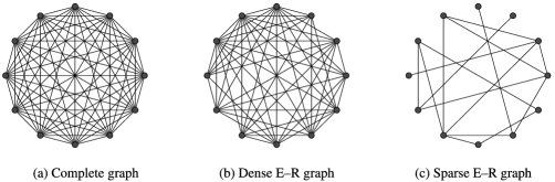
In Section 2 we review the well understood case when $G=K_{n}$, the $n$-clique or the complete graph on $n$ vertices, in which all pairs of distinct vertices are connected by an edge; see Figure 1(a). For suitable initial conditions $\xi$, convergence results for $\mu^{K_{n},\xi}$ and $X_{o}^{K_{n},\xi}$ in the context of interacting diffusion models go back more than half a century to the seminal works of McKean [59, 58], and fall under the rubric of mean-field limits. As briefly described in Section 2, under broad conditions, the limits, as $n\rightarrow\infty$, of both $\mu^{K_{n},\xi}$ and the law of $X_{o}^{K_{n},\xi}$ exist and coincide, and are described by a certain nonlinear stochastic process. More recent work has also considered interacting processes on certain dense random graph sequences. A generic example of a random graph is the so-called Erdős–Rényi graph $G(n,p_{n})$, which is a graph on $n$ vertices in which each pair of vertices has an edge with probability $p_{n}\in(0,1)$ independently of all other edges; see Figures 1(b) and 1(c) for realizations of $G(n,p_{n})$ with $n=12$ and $p_{n}=0.8$ and $p_{n}=0.25$, respectively. Motivated by the study of synchronization phenomena, the work [20] considers suitably scaled pairwise interacting diffusions on “dense” Erdős–Rényi graph $G(n,p_{n})$ sequences with divergent average degree ($np_{n}\rightarrow\infty$), and shows that the law of $X_{o}^{G_{n},\xi}$ converges to the same mean-field limit as in the complete graph case. The key idea is that in this regime, particles are only weakly interacting and become asymptotically independent, and thus the empirical measure behaves as in the i.i.d. case (1.2) described in Section 1.1.

The main focus of this article is on the complementary setting of interacting stochastic processes on sequences of sparse (possibly random) graphs, where the (average) degrees of vertices are uniformly bounded as $n\rightarrow\infty$. A typical example is the Erdős–Rényi graph $G(n,p_{n})$ sequence when $np_{n}\rightarrow c\in(0,1)$. There has been extensive analysis of various interacting stochastic processes on deterministic sparse graphs, originating with the work of Spitzer [72], followed by significant analysis of several Markovian models including the contact process, exclusion process, and voter model. These were first studied on the $d$-dimensional lattice (see the monographs [53, 54, 42, 28]) and then on $d$-regular trees (e.g., [66, 73]). More recent work has also considered processes on sparse random interaction graphs (see, e.g., [12, 20, 62, 39, 33, 6] for an incomplete list), but none of these latter works appear to address the main question listed above of autonomous characterization of the marginal dynamics of a typical particle. In fact, for interacting diffusions on the sequence of sparse Erdős–Rényi graphs $G_{n}=G(n,c/n)$, with $c\in(0,\infty)$, obtaining such a characterization has remained an important open question (e.g., see [20, p. 9]).

The sparse regime is more challenging because particles have strong interactions, neighboring particles remain correlated in the limit as $n\rightarrow\infty$, and the topology of the graph has a strong influence. Sections 3 and 4 describe recent progress that in particular provides a resolution of the open question in [20]. The article concludes in Section 5 with generalizations and open questions. The work on both mean-field models and various other aspects of interacting particle systems is so extensive that it will be impossible to be representative in this short article. Instead, I hope to just provide enough pointers for the reader to get a flavor of the classical results and set the context for more recent results. Monographs covering various aspects of interacting particles systems include [53, 54, 74, 7, 42, 45, 35, 21].

2. Classical mean-field results for interacting stochastic processes

Given a (simple, locally finite, undirected) graph $G=(V,E)$ and $v\in V$, we use $\mathrm{cl}_{G}(v):=\{v\}\cup\partial_{G}(v)$ to denote the closure of $v$ in $G$. Note that $|\mathrm{cl}_{G}(v)|$ is always finite, where $|A|$ denotes the cardinality of a set $A$. We now describe the dynamics of locally interacting diffusions and interacting jump processes. Rather than provide the most general setting, we make simplifying assumptions whenever convenient to illustrate the key issues.

2.1. Interacting diffusions

Given an initial condition $\xi=(\xi_{v})_{v\in V}\in\mathbb{R}^{V}$ with ${\mathbb{E}}[\xi_{v}^{2}]<\infty$ for every $v\in V$, consider the collection $X^{G,\xi}=\{X_{v}^{G,\xi}\}_{v\in V}$ of diffusive particles, indexed by the nodes of the graph $G$, that evolve according to the following coupled system of stochastic differential equations (SDEs):

$$dX_{v}^{G,\xi}(t)=b\bigl{(}t,X_{v}^{G,\xi}(t),\mu_{v}^{G,\xi}(t)\bigr{)}\,dt+dW_{v}(t),\quad X_{v}^{G,\xi}(0)=\xi_{v},\quad t>0,v\in V,\quad$$ (2.1)

where $(W_{v})_{v\in V}$ are i.i.d. standard Brownian motions independent of $(\xi_{v})_{v\in V}$, and for any vertex that is not isolated, $\mu_{v}^{G,\xi}(t)$ represents the local empirical measure of a neighborhood of $v$ at time $t\geq 0$,

$$\mu_{v}^{G,\xi}(t)=\frac{1}{|\partial_{G}(v)|}\sum_{u\in\partial_{v}}\delta_{X_{u}^{G,\xi}(t)},$$

and $b$ is a drift coefficient that is sufficiently regular to ensure that the SDE (2.1) has a unique weak solution. (When $v$ is isolated, the precise definition of $\mu_{v}^{G,\xi}$ is not so important; it can be set equal to an arbitrary quantity.)

A special case of interest is when $b$ has linear dependence on the measure term, say, of the form

$$b(t,x,\nu)=\int_{\mathbb{R}}\beta(t,x,y)\nu(dy),$$ (2.2)

for some interaction potential $\beta:\mathbb{R}_{+}\times\mathbb{R}^{2}\to\mathbb{R}$ that is symmetric in the last two variables. In this case, system (2.1) reduces to the following system of pairwise interacting diffusions:

$$dX_{v}^{G,\xi}(t)=\frac{1}{|\partial_{G}(v)|}\sum_{u\sim v}\beta\bigl{(}t,X_{v}^{G,\xi}(t),X_{u}^{G,\xi}(t)\bigr{)}dt+dW_{v}(t),\quad v\in V,t>0,$$ (2.3)

which models phenomena in different fields, including statistical physics and neuroscience [22, 69, 57]. The trajectories of each particle lie in the space $\mathcal{C}$ of continuous real-valued functions on $[0,\infty)$, which we endow with the topology of uniform convergence on compact sets.

2.2. Mean-field limits and nonlinear diffusion processes

Now consider the SDE (2.3) with $G=K_{n}$, the complete graph, and assume without loss of generality that $G$ has vertex set $\{1,\ldots,n\}$. We present a sufficient condition on the drift under which one can establish a standard mean-field result. Given any $p\geq 1$ and Polish space $E$, the Wasserstein-$p$ metric on $E$ is defined as follows:

$$\mathcal{W}_{E,p}(\nu,\tilde{\nu}):=\inf_{\pi}\biggl{(}\int_{E\times E}d^{p}(x,y)\pi(dx,dy)\biggr{)}^{1/p},$$ (2.4)

where the infimum is over all couplings $\pi$ of $\nu$ and $\tilde{\nu}$, namely probability measures $\pi$ on $E^{2}$ with first and second marginals $\nu$ and $\tilde{\nu}$, respectively. Let $\mathcal{P}^{p}(E)$ be the space of probability measures on $E$ equipped with the Wasserstein-$p$ metric $\mathcal{W}_{E,p}$.

Assumption 2.1.

Suppose that $b$ is bounded and for every $t>0$, the map $\mathbb{R}\times\mathcal{P}^{2}(\mathbb{R})\ni(x,\nu)\mapsto b(t,x,\nu)\in\mathbb{R}$ is Lipschitz continuous, uniformly with respect to $t$ in compact subsets of $\mathbb{R}_{+}$.

Note that Assumption 2.1 is satisfied when the drift $b$ is of the form (2.2), where the interaction potential $\beta$ is such that $\mathbb{R}^{2}\ni(x,y)\to\beta(t,x,y)$ is Lipschitz continuous and bounded, uniformly with respect to $t$ in compact subsets of $\mathbb{R}_{+}$.

Theorem 2.2.

Suppose Assumption 2.1 holds, and there exists $\mu_{o}\in\mathcal{P}^{2}(\mathbb{R})$ such that the initial conditions $(\xi^{n}_{i})_{i=1,\ldots,n}$, $n\in{\mathbb{N}}$, satisfy

$${\mathbb{E}}\Biggl{[}\mathcal{W}_{\mathbb{R},2}\Biggl{(}\frac{1}{n}\sum_{i=1}^{n}\delta_{\xi_{i}^{n}},\mu_{o}\Biggr{)}\Biggr{]}\rightarrow 0\quad\mbox{as }n\rightarrow\infty.$$ (2.5)

Then there is a unique strong solution to the SDE

$$dX_{o}(t)=b\bigl{(}t,B(t),\mu(t)\bigr{)}\,dt+dB(t),\quad\mu(t)=\mathscr{L}\bigl{(}X_{o}(t)\bigr{)},\quad t>0,$$ (2.6)

with $\mathscr{L}(X_{o}(0))=\mu_{0}$. Moreover, if for each $n\in{\mathbb{N}}$, $X^{n}:=X^{K_{n},\xi^{n}}$ is the unique solution to the SDE (2.1), then the global empirical measure $\mu^{n}:=\mu^{K^{n},\xi^{n}}$ defined in (1.4) satisfies

$$\lim_{n\rightarrow\infty}{\mathbb{E}}\Bigl{[}\sup_{s\in[0,t]}\mathcal{W}_{\mathbb{R},2}\bigl{(}\mu^{n}(s),\mu(s)\bigr{)}\Bigr{]}=0,\quad\forall t>0.$$ (2.7)

Furthermore, for any $k\in\mathbb{N}$ and $t>0$, the law of $(X_{1}^{n}(t),\ldots,X_{k}^{n}(t))$ converges weakly to the product $(\mu(t))^{\otimes k}$, that is, for all bounded continuous functions $f_{i}:\mathbb{R}\to\mathbb{R}$, $i=1,\ldots,k$,

$$\lim_{n\rightarrow\infty}{\mathbb{E}}\bigl{[}f_{1}\bigl{(}X_{1}^{n}(t)\bigr{)}\ldots f_{k}\bigl{(}X_{k}^{n}(t)\bigr{)}\bigr{]}=\prod_{i=1}^{k}\int_{\mathbb{R}}f_{i}(x)\mu(t)(dx).$$ (2.8)

If there were no interaction, $b\equiv 0$, then the theorem would simply be a (functional) strong law of large numbers result. However, even when $b\not\equiv 0$, the particles are only weakly interacting because the symmetry of the interaction ensures that the influence of any particle on the drift of another particle is $O(1/n)$, which vanishes in the limit. The property (2.8) that any finite subset of random variables from $\{X^{n}_{i}(t),i=1,\ldots,n\}_{n\in\mathbb{N}}$ are asymptotically independent is referred to as chaoticity, and is well known to be equivalent to the convergence of $\mu^{n}(t)$ to a deterministic law [74, Proposition 2.2]. Now, (2.5) implies that the initial conditions are chaotic. Thus Theorem 2.2 asserts that the dynamics are such that this chaoticity also holds for positive times $t>0$, a phenomenon referred to as propagation of chaos. In turn, this leads to an autonomous description of the limiting marginal process $X_{o}$, which is a Markov process whose infinitesimal evolution at any time $t$ also depends on its own law $\mu(t)$ at that time. As a result, the forward Kolmogorov equation (or master equation), which is the partial differential equation (PDE) describing the evolution of the marginal law $\mu$, is nonlinear. Consequently, such a process is referred to as a nonlinear Markov process. When the drift has the form (2.2), under suitable conditions it can be shown that the law $\mu(t)$ is absolutely continuous with respect to Lebesgue measure and that its density satisfies the granular media equation [59]. Thus, PDE techniques can be useful for studying nonlinear Markov processes (see, e.g., [4]).

There are many different approaches to establishing mean-field limits, including PDE analysis, fixed point arguments, martingale techniques and stochastic coupling constructions. First, one needs to establishing well-posedness of the nonlinear SDE (2.6). An analytical approach to this problem entails proving uniqueness of the nonlinear PDE describing the evolution of the marginal law. Another, more probabilistic, approach is to first consider the mapping that takes any continuous measure flow $t\mapsto\nu(t)\in\mathcal{P}^{2}(\mathbb{R})$ to the measure flow $t\mapsto\mathscr{L}(X^{\nu}(t))$, where $X^{\nu}$ is the unique solution to the SDE in (2.6) when $\mu$ is replaced with $\nu$. Observing that the flow $t\mapsto\mathscr{L}(X_{o}(t))$ must be a fixed point for this mapping, well-posedness is equivalent to uniqueness of the fixed point of this mapping. The latter can be established by showing the mapping is a contraction by exploiting the Lipschitz continuity of the drift. Given well-posedness, the coupling approach to proving convergence proceeds by first defining $\bar{X}^{n}$ to be the $n$-dimensional process whose every coordinate is an independent copy of the nonlinear process $X_{o}$. Then one couples this process with the original process $X^{n}$ so that they are both driven by the same Brownian motions. Using Itô’s formula, the Lipschitz condition on the drift and standard estimates, one can then show that the $\mathcal{W}_{\mathbb{R},2}$ distance between the empirical measures of $X^{n}$ and $\bar{X}^{n}$ vanishes as $n\rightarrow\infty.$ Since the strong law of large numbers ensures that the empirical measure of the latter converges to the law of $X_{o}$, which is equal to $\mu$, this concludes the proof. An alternative approach to proving convergence is to first use the generator of the Markov process $X^{n}$ to identify martingales involving the empirical measure process $\mu^{n}$, next show that the sequence $\{\mu^{n}\}$ is relatively compact (or tight), then characterize any subsequential limit satisfies what is known as a nonlinear martingale problem, and finally establish well-posedness of the latter [63, 34].

Remark 2.3.

One can consider more general dynamics where both the drift and diffusion coefficients are functions of the current state and the empirical measure process, as well as non-Markovian versions that depend on the history of the process.

2.3. Interacting jump processes and their mean-field limits

2.3.1. Description of dynamics

We will also be interested in interacting pure jump processes, which describe models in statistical physics, engineering, epidemiology and the dynamics of opinion formation [54, 7]. For concreteness, consider the voter model [54] that aims to capture opinion dynamics, in which each particle takes values in the state space $\mathcal{X}=\{0,1\}$ that represents two possible opinions. The allowed transitions or jump directions of a particle lie in the set $\mathcal{J}=\{1,-1\}$. The rate at which any particle changes its opinion is equal to the fraction of its neighbors with the opposite opinion. Note that the dependence of the rate on the neighboring states is symmetric. More generally, when the state of the system is $(x_{v})_{v\in V}$, the jump rate of a particle at $v$ could be a more complicated symmetric functional of the neighboring states $(x_{u})_{u\sim v}$ and also depend on time $t$, in addition to its own state $x_{v}$. This symmetric dependence on neighboring states is most succinctly captured by saying the rate is a functional of the unnormalized empirical measure $\theta_{v}=\sum_{u\sim v}\delta_{x_{u}}$ of the neighboring states. Note that $\theta_{v}$ lies in the space $\mathcal{M}(\mathcal{X})$ of locally finite nonnegative integer-valued measures on $\mathcal{X}$.

In the general setup, we consider a finite state space $\mathcal{X}$, a subset $\mathcal{J}\subset\{i-j:i,j\in\mathcal{X}\}$ of possible jump directions, and a collection of jump rate functions $\bar{r}_{j}:\mathbb{R}_{+}\times\mathcal{X}\times\mathcal{M}(\mathcal{X})\to\mathbb{R}_{+}$, $j\in\mathcal{J}$. Given a (simple) finite graph $G=(V,E)$ and initial condition $\xi=(\xi_{v})_{v\in V}\in{\mathcal{X}}^{V}$, the $\mathcal{X}^{V}$-valued process representing the configuration of the associated IPS evolves according to the following system of (jump) SDEs:

$$X^{G,\xi}_{v}(t)=\xi_{v}+\sum_{j\in\mathcal{J}}j\int_{(0,t]\times\mathbb{R}_{+}}\mathbb{I}_{\{r\leq\bar{r}_{j}(s,X^{G,\xi}_{v}(s-),\theta_{v}^{G,\xi}(s-))\}}N_{v}(ds,dr),\quad t\geq 0,v\in V,$$ (2.9)

where $(N_{v})_{v\in V}$, are i.i.d. Poisson random measures on $\mathbb{R}_{+}^{2}$ with intensity measure $\mathrm{Leb}^{2}$, where $\mathrm{Leb}$ represents Lebesgue measure on $\mathbb{R}$, and for each $s\geq 0$, $\theta^{G,\xi}_{v}(s)$ is the random (unnormalized) empirical measure corresponding to the states of the particles in the neighborhood of $v$ at time $s$:

$$\theta_{v}^{G,\xi}(s):=\sum_{u\sim v}\delta_{X^{G,\xi}_{u}(s)},\quad v\in V,s\geq 0.$$ (2.10)

The SDE (2.9) captures a simple evolution. For any $j\in{\mathcal{J}}$ and time $t$, the particle at a node $v$ makes a transition from its state $X^{G,\xi}_{v}(t-)$ to $X^{G,\xi}_{v}(t-)+j$ at a rate $\bar{r}_{j}(t,x,\theta_{v}^{G,\xi}(t-))$ that depends on the current time, the state of the node just prior to the current time, and symmetrically on the states of neighboring nodes just prior to the current time, as encoded by $\theta_{v}^{G,\xi}(t-)$. Use of the unnormalized measure $\theta_{v}^{G,\xi}(t)$ instead of the empirical measure allows one to capture a broader class of models in which jump rates depend on the number of neighboring nodes in particular states (and not just their fractions), as is the case for models like the contact process [54]. Note that the trajectory of each particle lies in the càdlàg space $\mathcal{D}$ of right continuous ${\mathcal{X}}$-valued functions on $[0,\infty)$ that have finite left limits on $(0,\infty)$.

The solution $X^{G,\xi}$ to the jump SDE (2.9) is a Markov jump process and so its law can also be characterized via the associated infinitesimal generator [53]: for functions $f:\mathcal{X}^{V}\mapsto\mathbb{R}$,

$$\mathcal{A}_{t}f(x) =\lim_{h\downarrow 0}\frac{\mathbb{E}[f(X_{t+h}^{G,\xi})-f(X_{t}^{G,\xi})|X_{t}^{G,\xi}=x]}{h}$$

$$=\sum_{j\in\mathcal{J},v\in V}\bar{r}_{j}\biggl{(}t,x_{v},\sum_{u\sim v}\delta_{x_{u}}\biggr{)}\bigl{[}f(x+je_{v})-f(x)\bigr{]},\quad t>0,x\in\mathcal{X}^{V},$$

where $e_{v}\in\{0,1\}^{V}$ is the vector with $1$ in the $v$th coordinate and $0$ elsewhere. However, the jump SDE representation in (2.9) is more convenient for generalizations to non-Markovian processes (see [30]). Furthermore, the jump SDE formulation is also better suited to describing the form of limiting marginal dynamics on sparse graphs, as described in Section 4.4.

2.3.2. Mean-field limits and nonlinear jump processes

Mean-field results analogous to Theorem 2.2 also hold in the jump setting under the following regularity assumption on the jump rate functions:

Assumption 2.4.

For each $j\in\mathcal{J}$, the jump rate function takes the form $\tilde{r}_{j}(t,x,\theta)=\hat{r}_{j}(t,x,\frac{1}{\theta(\mathcal{X})}\theta)$ when $\theta({\mathcal{X}})\neq 0$, and $\tilde{r}_{j}(t,x,\theta)=0$ otherwise, where the function $\hat{r}_{j}:\mathbb{R}\times\mathcal{X}\times\mathcal{P}^{1}(\mathcal{X})\mapsto\mathbb{R}_{+}$ is such that ${\mathcal{P}}^{1}({\mathcal{X}})\ni\nu\mapsto\hat{r}(t,x,\nu)$ is Lipschitz continuous, uniformly for $x\in{\mathcal{X}}$ and $t$ in compact subsets of $\mathbb{R}_{+}$.

Assumption 2.4 reflects the fact that in the mean-field setting, the dependence of the jump rates on the neighboring particles must be a sufficiently regular function of the usual (normalized) empirical measure. The following result is established in [63, Theorem 2]; see also [45].

Theorem 2.5.

Suppose Assumption 2.4 holds and the initial conditions are chaotic, that is, $\frac{1}{n}\sum_{i=1}^{n}\delta_{\xi_{i}^{n}}$ converges in the total variation metric to a deterministic limit $\mu_{0}$, then $\mu^{K_{n},\xi^{n}}(t)$ converges weakly to $\mathscr{L}(X_{o}(t))$ where $X_{o}(t)=X^{\mu_{0}}(t)$, $t\geq 0$, is the unique solution to the following nonlinear jump SDE: $\mathscr{L}(\mathcal{X}_{o}(0))=\mu_{0}$, and for $t\geq 0$,

$$X_{o}(t) =X_{o}(0)+\sum_{j\in\mathcal{J}}j\int_{(0,t]\times\mathbb{R}_{+}}\mathbb{I}_{\{r\leq\bar{r}_{j}(s,X_{o}(s-),\mu(s-))\}}N(ds,dr),$$ (2.11)

$$\mu(t) =\mathscr{L}\bigl{(}X_{o}(t)\bigr{)},$$

where $N$ is a Poisson process on $\mathbb{R}^{2}_{+}$ with intensity $\mathrm{Leb}^{2}$, independent of $X_{o}(0)$. Furthermore, for any $k\in\mathbb{N}$, the law of $(X_{1}^{K_{n},\xi},\ldots,X_{k}^{K_{n},\xi})$ on $\mathcal{D}^{k}$ converges weakly to $(\mathcal{L}(X_{o}))^{\otimes_{k}}$.

Just as the evolution of the law of the mean-field diffusion limit in (2.6) can be characterized by a nonlinear PDE, the evolution of the law of the nonlinear jump process $X_{o}$ in (2.11) can be characterized as the unique solution to its forward equation, which is now a nonlinear integrodifferential equation.

Remark 2.6.

Theorems 2.2 and 2.5 are meant to only provide a flavor of mean-field results. While a survey of mean-field limits is not the current focus, it is worth mentioning that in both the diffusive and jump process settings, one can obtain mean-field limits under weaker assumptions and for much more general dynamics where the diffusion coefficient is also a function of the current state and empirical measure process, as well as non-Markovian versions where the drift coefficient or jump rates depend on the history of the process (see, e.g., [60] for propagation of chaos results on interacting non-Markovian jump diffusions and [3] for a large deviations analysis of non-Markovian weakly interacting diffusions).

Figure 2. Simulations and mean-field (MF) approximations for the voter model on a $3$-tree.

2.4. Limitations of mean-field approximations

The mean-field limit theorems established in Theorems 2.2 and 2.5 indicate that the law of the nonlinear Markov processes $X_{o}$ in (2.6) and (2.11), respectively, can be used to approximate quantities of interest for interacting diffusions or jump processes on finite graphs. In particular, consider the voter model described in Section 2.3.1. Its jump rates take the explicit form

$$\bar{r}_{1}(t,x,\theta) =\frac{\mathbb{I}_{\{x=0\}}}{|\theta(\mathcal{X})|}\int_{\mathcal{X}}y\theta(dy),\quad\bar{r}_{-1}(t,x,\theta)=\frac{\mathbb{I}_{\{x=1\}}}{|\theta(\mathcal{X})|}{\int_{\mathcal{X}}(1-y)\theta(dy)}.$$

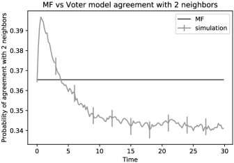
In this case, one would expect that the dynamics of $X_{o}$ in (2.11) with these reates could provide an approximation for the probability of agreement of any two neighboring particles in the voter model on a sufficiently large complete graph. However, for lack of a better alternative, mean-field approximations are used even for dynamics on other graphs. While these approximations may do reasonably well on dense graphs (where vertices have high degrees) [20], they can be very inaccurate on sparse graphs. Figure 2 plots the evolution of the probability that the state of the root agrees with precisely two of its neighbors for the voter model on a rooted $3$-regular tree with $9$ generations, given at time zero, each particle independently has an opinion $1$ with probability $0.3$. The vertical bars in Figure 2 provide confidence intervals for the simulation. The mean-field approximation assumes neighboring vertices are independent, and thus performs poorly. Ad hoc refinements of the mean-field approximation that take into account correlations also remain inaccurate in this setting. This strongly motivates the development of a convergence theory for the empirical distribution and marginal dynamics on sparse graph sequences that could lead to more principled approximations.

3. Interacting processes on sparse graphs: hydrodynamic limits

We now turn to interacting processes $(X^{G_{n},\xi^{n}})_{n\in\mathbb{N}}$ on sparse graph sequences $(G_{n})_{n\in\mathbb{N}}$ with initial conditions $(\xi^{n})_{n\in\mathbb{N}}$. Assume each $G_{n}$ is finite and $o_{n}$ is a vertex chosen uniformly at random from the vertices of $G_{n}$. Unlike in the case of the complete graph (or even dense graph sequences), the degree of a vertex remains bounded and so neighboring vertices do not become asymptotically independent. Thus, the number of neighbors becomes important and so it is clear that one cannot expect $(X^{G_{n},\xi^{n}}_{o_{n}})_{n\in\mathbb{N}}$ to have a limit just by sending the number of vertices $n$ to infinity, without imposing any additional consistency requirements on the graphs in the sequence. This leads to the following questions:

1. For what graph sequences $(G_{n})_{n\in{\mathbb{N}}}$ would one expect $(X^{G_{n},\xi^{n}}_{o_{n}})_{n\in{\mathbb{N}}}$ to have a limit?

2. For such sequences, will $(\mu^{G_{n},\xi^{n}})_{n\in{\mathbb{N}}}$ converge to a deterministic limit?

3. When $(\mu^{G_{n},\xi^{n}})_{n\in{\mathbb{N}}}$ converges to a deterministic limit, will this limit always coincide with the limit law of $X^{G_{n},\xi^{n}}_{o_{n}}$?

4. Is there an autonomous reduced-dimension description of the limit of the marginal $X^{G_{n},\xi^{n}}_{o_{n}}$ whenever this limit exists?

In light of the first question above, we review a natural notion of convergence of sparse graphs called local convergence in Section 3.1. This notion was used to study asymptotic properties of static models (Gibbs measures) of discrete-valued marked random graphs in [21].

3.1. Local convergence of sparse graph sequences

Given a graph $G=(V,E)$ and two vertices $u,v\in V$, a path of length $n$ between $u$ and $v$ is a sequence $u=u_{0},u_{1},\ldots,u_{n}=v$ such that $u_{i-1}\sim u_{i}$ for every $i=1,\ldots,n$. A graph is said to be connected if there exists a finite path between any two vertices and the graph distance between two vertices is the minimum length of a path between them. A rooted graph $(G,o)$ is a graph $G=(V,E)$ with a special vertex $o\in V$, referred to as the root. A useful notion of convergent sequences of (connected) rooted sparse graphs is that of local convergence, which was introduced by Benjamini and Schramm [5]. Other references on local convergence include [8, 1]. We first introduce some terminology that is required to define local convergence. An isomorphism from one rooted graph $(G_{1},o_{1})$ to another $(G_{2},o_{2})$ is a bijection $\varphi$ from the vertex set of $G_{1}$ to that of $G_{2}$ such that $\varphi(o_{1})=o_{2}$ and such that $(u,v)$ is an edge in $G_{1}$ if and only if $(\varphi(u),\varphi(v))$ is an edge in $G_{2}$. Two rooted graphs are said to be isomorphic if there exists an isomorphism between them. Let $\mathcal{G}_{*}$ denote the set of isomorphism classes of connected rooted graphs. We will also need to consider convergence of graphs that carry ”marks” representing the initial condition or trajectory of the state dynamics at that vertex. With that in mind, given a Polish space $\mathcal{S}$, we define a $\mathcal{S}$-marked rooted graph to be a tuple $(G,x,o)$, where $(G,o)$ is a rooted graph and $x=(x_{v})_{v\in G}\in\mathcal{S}^{G}$ is a vector of marks, indexed by the vertices of $G$. We say that two marked rooted graphs $(G_{1},x^{1},o_{1})$ and $(G_{2},x^{2},o_{2})$ are isomorphic if there exists an isomorphism $\varphi$ from the rooted graph $(G_{1},o_{1})$ to the rooted graph $(G_{2},o_{2})$ that maps the marks of $(G_{1},o_{1})$ to the marks of $(G_{2},o_{2})$ (i.e., for which $x^{2}_{\varphi(v)}=x^{1}_{v}$ for all $v\in G$). Let $\mathcal{G}_{*}[\mathcal{S}]$ denote the set of isomorphism classes of $\mathcal{S}$-marked rooted graphs.

We now define the topologies of local convergence on the spaces $\mathcal{G}_{*}$ and $\mathcal{G}_{*}[\mathcal{S}]$. For $r\in{\mathbb{N}}$ and $(G,o)\in\mathcal{G}_{*}$, let $B_{r}(G,o)$ denote the induced subgraph of $G$ (rooted at $o$) containing those vertices with (graph) distance at most $r$ from the root $o$. The distance between $(G_{1},o_{1})$ and $(G_{2},o_{2})$ in $\mathcal{G}_{*}$ is defined to be $1/(1+\bar{r})$, where $\bar{r}$ is the supremum over $r\in{\mathbb{N}}_{0}$ such that $B_{r}(G_{1},o_{1})$ and $B_{r}(G_{2},o_{2})$ are isomorphic, where we interpret $B_{0}(G_{i},o_{i})=\{o_{i}\}$. Now, let $d$ denote a metric that induces the Polish topology on $\mathcal{S}$. We then metrize $\mathcal{G}_{*}[\mathcal{S}]$ by similarly defining the distance between two $\mathcal{S}$-marked graphs $(G_{i},x^{i},o_{i})$, $i=1,2$, to be $1/(1+\bar{r})$, where now $\bar{r}$ is the supremum over $r\in{\mathbb{N}}_{0}$ such that there exists an isomorphism $\varphi$ from $B_{r}(G_{1},o_{1})$ to $B_{r}(G_{2},o_{2})$ for which $d(x^{1}_{v},x^{2}_{\varphi(v)})\leq 1/r$ for all $v\in B_{r}(G_{1},o_{1})$. Under the respective topologies, $\mathcal{G}_{*}$ and $\mathcal{G}_{*}[\mathcal{S}]$ are Polish spaces (see [8, Lemma 3.4] or [47, Appendix A]). For any Polish space $\mathcal{S}$, let $C_{b}(\mathcal{S})$ denote the space of bounded continuous functions on $S$.

We will always assume the spaces $\mathcal{G}_{*}$ and $\mathcal{G}_{*}[\mathcal{S}]$ are equipped with their Borel $\sigma$-algebras. One can then talk about weak convergence or convergence in distribution of random graphs and random marked graphs as random elements in $\mathcal{G}_{*}$ or $\mathcal{G}_{*}[\mathcal{S}].$ Specifically, a sequence of random $\mathcal{G}_{*}$-valued random elements $\{(G_{n},o_{n})\}$ is said to converge in distribution in the local weak sense to a $\mathcal{G}_{*}$-valued limit $(G,o)$ if for every bounded continuous function $f:\mathcal{G}_{*}\rightarrow\mathbb{R}$, $\mathbb{E}[f(G_{n},o_{n})]\rightarrow\mathbb{E}[f(G,o)].$ Likewise, convergence in distribution in the local weak sense of (isomorphism classes of) random $\mathcal{S}$-marked graphs is equivalent to weak convergence on the space $\mathcal{G}_{*}[\mathcal{S}]$.

(a) $\longrightarrow$         $\vdots\ \ \$ $\vdots\ \ \$
(b) $\longrightarrow$ $\hphantom{x}\quad\quad\quad\quad\ \ \ \vdots\quad\quad\quad\quad\quad\quad\ \ \vdots$

Figure 3. Local convergence: (a) cycle to infinite line; (b) Erdős–Rényi graph to a UGW tree.

Remark 3.1.

Figure 3 illustrates two generic examples of locally convergent graph sequences. Let $G_{n}$ be the $n$-cycle, which is the connected graph on $n$ vertices where every vertex has degree $2$, along with the root $o_{n}$ chosen uniformly at random from the $n$ vertices. Then $(G_{n},o_{n})$ converges weakly in $\mathcal{G}_{*}$ to a infinite line graph rooted at some fixed vertex; see Figure 3(a). A less trivial example is illustrated in Figure 3(b). Given $c\in(0,\infty)$, the sequence of Erdős–Rényi graphs $G(n,c/n)$ converges in distribution in the local weak sense to the Galton–Watson (GW) tree with offspring distribution given by the Poisson($c$) distribution. The latter is an example of a unimodular Galton–Watson (UGW) tree, which is defined as follows. Given a probability distribution $\rho$ on ${\mathbb{N}}\cup\{0\}$ that has finite nonzero first moment, that is, satisfies $0<\sum_{k\in{\mathbb{N}}}k\rho(k)<\infty$, the random tree UGW($\rho$) has a root whose neighborhood size is distributed according to $\rho$. The neighbors of the vertices are referred to as the offspring of the root and form the first generation of the tree. Recursively, for $n\geq 1$, each vertex in the nth generation of the tree has an independent random number of offspring (equivalently, neighbors that are further away from the root than itself) with distribution $\widehat{\rho}$

$$\hat{\rho}(k)=\frac{(k+1)\rho(k+1)}{\sum_{n\in{\mathbb{N}}}n\rho(n)},\quad k\in{\mathbb{N}}\cup\{0\}.$$ (3.1)

The $(n+1)$th generation of the tree is comprised of all offspring of vertices in the $n$th generation. It is easy to verify that if $\rho$ is a Poisson distribution, then $\hat{\rho}=\rho$. Hence, a Galton–Watson tree with a Poisson($c$) offspring distribution is in fact a UGW (Poisson($c$)) distribution. Another special case is the $\kappa$-regular tree, for $\kappa\geq 2$, which is given by $\mathbb{T}_{\kappa}:=$ UGW ($\delta_{\kappa}$). UGW trees are in a sense canonical objects since they arise as local weak limits of many sparse random graph sequences including Erdős–Rényi graphs, configuration models and preferential attachment graphs; see [47, Section 2.2.4] for further discussion of these examples.

To extend this notion of convergence to graphs that are not necessarily connected, given an (unrooted) graph $G=(V,E)$ and a vertex $v\in V$, define $\mathsf{C}_{v}(G)\in\mathcal{G}_{*}$ to be the isomorphism class of the connected component of $G$ that contains $v$, with $v$ as its root. Furthermore, when $G$ is finite, we let $o$ denote a random vertex of $G$ chosen uniformly from the set $V$, in which case $\mathsf{C}_{o}(G)$ denotes the connected component of that random vertex.

Definition 3.2.

A sequence of finite (random) graphs $\{G_{n}\}$ is said to converge in distribution in the local weak sense to $G$ if

$$\lim_{n\to\infty}{\mathbb{E}}\biggl{[}\frac{1}{|G_{n}|}\sum_{v\in G_{n}}f\bigl{(}\mathsf{C}_{v}(G_{n})\bigr{)}\biggr{]}={\mathbb{E}}\bigl{[}f(G)\bigr{]},\quad\forall f\in C_{b}(\mathcal{G}_{*}).$$ (3.2)

A sequence of finite (random) graphs $\{G_{n}\}$ is said to converge in probability in the local weak sense to $G$ if for every $\varepsilon>0$,

$$\lim_{n\to\infty}\mathbb{P}\biggl{(}\biggl{|}\frac{1}{|G_{n}|}\sum_{v\in G_{n}}f\bigl{(}\mathsf{C}_{v}(G_{n})\bigr{)}-{\mathbb{E}}\bigl{[}f(G)\bigr{]}\biggr{|}>\varepsilon\biggr{)}\rightarrow 0,\quad\forall f\in C_{b}(\mathcal{G}_{*}).$$ (3.3)

Analogously, given a marked (unroooted, not necessarily connected) graph $(G,x)$, $\mathsf{C}_{v}((G,x))$ denotes the connected component of $G$ containing $v$, with $v$ as its root and with the corresponding marks. The notions of convergence in distribution and in probability in the local weak sense for marked graphs are defined in an exactly analogous fashion as Definition 3.2, with $\mathsf{C}_{v}((G_{n},x^{n}))$, $\mathsf{C}_{v}((G_{,}x))$ and $(G,x)$ in place of $\mathsf{C}_{v}(G_{n})$, $\mathsf{C}_{v}(G)$ and $G$, respectively. For both unmarked and marked graphs, convergence in probability clearly implies convergence in distribution. We will use the same notation for graphs and their isomorphism classes and often omit the root from the notation and simply refer to $G\in\mathcal{G}_{*}$ rather than $(G,o)\in\mathcal{G}_{*}$.

Remark 3.3.

Given any sequence of random graphs $\{G_{n}\}_{n\in{\mathbb{N}}}$ that converges (either in distribution or in probability) in the local weak sense to a limit graph $G$, if $x^{n}=(x^{n}_{v})_{v\in G_{n}}$ are i.i.d. marks on some Polish space $\mathcal{S}$ with the same distribution irrespective of $n$, then it is easy to show that the marked graph sequence $\{(G_{n},x^{n})\}_{n\in{\mathbb{N}}}$ also converges (in the same local weak sense as the unmarked counterparts) to $(G,x)$, where $x=(x_{v})_{v\in G}$ is i.i.d. with the same distribution. In fact, as shown in [47, Proposition 2.16], convergence of the marked graph sequence holds for the larger class of possibly dependent marks distributed according to a Gibbs measure on the graph with respect to a fixed pairwise interaction functional.

3.2. Hydrodynamic limits

3.2.1. Interacting Diffusion processes

We now address Q1–Q3 raised at the beginning of Section 3. The first result below states that if a sequence of graphs marked with initial conditions converges (either in probability or in distribution) in the local weak sense to a limit graph, then the graphs marked with the trajectories that solve the corresponding SDE also converge to the limit graph in the same sense. The result also characterizes the limit of the global empirical measure under suitable conditions.

Theorem 3.4.

Suppose Assumption 2.1 holds, and the sequence $\{(G_{n},\xi^{n})\}_{n\in{\mathbb{N}}}$ of (not necessarily connected, finite) random marked graphs converges in distribution in the local weak sense to a $\mathcal{G}_{*}[B_{r}(\mathbb{R})]$-valued limit $(G,\xi)$ for some $r>0$. Also, for each $n\in{\mathbb{N}}$, let $X^{G_{n},\xi^{n}}$ be the solution to the SDE (2.3) with initial data $(G_{n},\xi^{n})$ and let $X^{G,\xi}$ be the unique weak solution to the SDE (2.3) on the limit graph $(G,\xi)$. Then $\{(G_{n},X^{G_{n},\xi^{n}})\}_{n\in{\mathbb{N}}}$ converges in distribution in the local weak sense to the $\mathcal{G}_{*}[\mathcal{C}]$-valued element $(G,X^{G,\xi})$. In particular, $\{X^{G_{n},\xi^{n}}_{o_{n}}\}_{n\in{\mathbb{N}}}$ converges weakly to $X^{G,\xi}_{o}$. Moreover, if $\{(G_{n},\xi^{n})\}_{n\in{\mathbb{N}}}$ converges in probability in the local weak sense to $(G,\xi)$, then $\{(G_{n},X^{G_{n},\xi^{n}})\}_{n\in{\mathbb{N}}}$ also converges in probability in the local weak sense to $(G,X^{G,\xi})$ and additionally, $\{\mu^{G_{n},\xi^{n}}\}_{n\in{\mathbb{N}}}$ converges weakly to the law of $X_{o}^{G,\xi}$.

This result follows from [47, Theorems 3.3 and 3.7], which establish this result for more general, possibly non-Markovian diffusive dynamics. A version of the first assertion of the above theorem was also established for a slightly different class of interacting diffusions in [65]. Theorem 3.4 can be seen as establishing continuity in the local weak topology of the dynamics with respect to the initial data, comprising the graph marked with initial conditions. It also provides conditions under which the empirical measure can be shown to have a deterministic limit (equivalently, hydrodynamic limit) that additionally coincides with the limit law of the root particle, thus answering in the affirmative Q2 and Q3 at the beginning of Section 3. As discussed earlier, on complete graphs the analogous phenomena holds due to asymptotic independence of the trajectories of any two particles. In contrast, in the sparse regime, neighboring particles remain dependent in the limit. Instead, the proof relies on showing that the trajectories on finite neighborhoods of two independent vertices, both chosen uniformly at random from the graph become asymptotically independent in the limit. The latter property relies on a certain correlation decay property of the dynamics in the spirit of (1.3); see [47, Lemma 5.2] for details.

However, it should be emphasized that in the sparse regime the deterministic hydrodynamic limit result holds only when the initial data converges in the stronger sense of convergence in probability in the local weak sense. Indeed, as shown in [47, Theorems 3.9 and 6.4], the limiting empirical measure can be stochastic when the initial data only converges in distribution in the local weak sense. In particular, fix $c\in(0,\infty)$ and suppose $\tilde{G}_{n}$ is the graph obtained by taking the connected component of a vertex chosen uniformly at random from the Erdős–Rényi graph $G(n,c/n)$, and setting the root to be that chosen vertex. Also, let the initial conditions $\xi^{n}=\{\xi^{n}_{v}\}_{v\in G_{n}}$ be i.i.d. with common distribution $\gamma$, and let $\tilde{\xi}^{n}$ denote the restriction of the initial conditions to $\bar{G}_{n}$. Then both $\{(G_{n},\xi^{n})\}_{n\in{\mathbb{N}}}$ and $\{(\tilde{G}_{n},\tilde{\xi}^{n})\}_{n\in{\mathbb{N}}}$ converge in distribution in the local weak sense to $(G,\xi)$, where $\xi=(\xi_{v})_{v\in V}$ is i.i.d. with distribution $\gamma$, and $G=\mathcal{T}:=\mathrm{UGW}(\mathrm{Poiss}(c))$. However, whereas $\mu^{G_{n},\xi}$ converges weakly to $\mathcal{L}(X_{o}^{\mathcal{T},\xi})$, the law of the dynamics at the root vertex in $\mathcal{T}$, $\mu^{\tilde{G}_{n},\tilde{\xi}^{n}}$ converges weakly to the following random limit $\tilde{\mu}^{\mathcal{T},\xi}$ given by

$$\tilde{\mu}^{\mathcal{T},\xi}:=\begin{cases}\mu^{\mathcal{T},\xi}&\mbox{on the event }|\mathcal{T}|<\infty,\\ \mathrm{Law}\bigl{(}X_{o}^{\mathcal{T},\xi}\mid|\mathcal{T}|=\infty\bigr{)}&\mbox{on the event }|\mathcal{T}|=\infty.\end{cases}$$

This limit is truly stochastic because, as is well known from the elementary theory of branching processes [2], there is always a positive probability for the UGW tree $\mathcal{T}$ to be finite (and there is a positive probability of $\mathcal{T}$ being infinite only when $c>1$). Furthermore, there also exist examples that show that even when the limiting empirical measure is deterministic, it need not coincide with the law of the root particle in the limit. For example, this can occur if the graph itself is not homogeneous and the root is not chosen uniformly at random from the vertices of the graph (see, e.g., [47, Section 3.6]). The above discussion shows that the existence and nature of the hydrodynamic limit is far more subtle in the sparse regime than in the case of complete or dense graphs, even for diffusive dynamics.

3.2.2. Interacting jump processes

In the setting of jump processes, additional subtleties arise. Whereas in the diffusion setting, Assumption 2.1 ensures that the drift of a particle at a node $v$ experiences only an $O(1/|\partial v|)$ effect when there is a perturbation in the state of a neighboring particle, an analogous assumption would be too stringent to cover most jump models of interest on sparse graphs. In the latter case, the effect of a neighboring particle on the jump intensity at a vertex either remains constant or $O(1)$ as in the voter model, or grows with the degree of the vertex in many other models, including the contact process (see [54]). It is precisely to accommodate such a dependence that the jump intensity $\bar{r}_{j}$ in (2.9) is expressed as a function of the unnormalized sum of the Dirac masses at neighboring states introduced in (2.10), rather than the normalized empirical measure. For hydrodynamic limits on sparse graphs, it will suffice to impose the following mild assumption on the rates.

Assumption 3.5.

For every $T>0$, suppose there exist constants $C_{k,T},k\in{\mathbb{N}}$, such that $k\mapsto C_{k,T}$ is nondecreasing and for every $j\in\mathcal{J}$, $\sup_{x\in\mathcal{X},t\in[0,T]}\bar{r}_{j}(t,x,\theta)\leq C_{\theta(\mathcal{X}),T}$.

Note that in the jump SDE (2.9) describing the dynamics, the third argument $\theta$ of $\bar{r}_{j}$ is equal to the unnormalized empirical measure of the states of the neighbors of a vertex, as defined in (2.10). Thus, $\theta(\mathcal{X})$ irepresents the degree of the vertex and Assumption 3.5 allows the uniform bound on the jump rates at a vertex to grow with the degree of a vertex.

We now state an analog of Theorem 3.4 for jump diffusions. Recall the definition of a UGW tree given in Remark 3.1.

Theorem 3.6.

Suppose Assumption 3.5 holds, and the sequence $\{(G_{n},\xi^{n})\}_{n\in{\mathbb{N}}}$ of (not necessarily connected, finite) random rooted marked graphs converges in probability in the local weak sense to a limit $(G,\xi)$, where $G$ is a UGW($\rho$) tree with $\rho$ having finite, strictly positive first and second moments. For each $n\in{\mathbb{N}}$, let $X^{G_{n},\xi^{n}}$ be the solution to the jump SDE (2.9) with initial data $(G_{n},\xi^{n})$, and let $X^{G,\xi}$ be the unique strong solution to the SDE (2.9) on the limit graph $(G,\xi)$. Then $\{(G_{n},X^{G_{n},\xi^{n}})\}_{n\in{\mathbb{N}}}$ converges in probability in the local weak sense to the $\mathcal{G}_{*}[\mathcal{D}]$-valued element $(G,X^{G,\xi})$. Furthermore, $\{\mu^{G_{n},\xi^{n}}\}_{n\in{\mathbb{N}}}$ converges weakly to the law of $X_{o}^{G,\xi}$.

This theorem follows from more general results established in [30, Theorem 4.8 and Corollary 5.16]. As in the diffusion case, the proof of the theorem involves establishing continuity properties of the dynamics with respect to the graph and initial condition as well as a correlation decay property. However, the proofs of these properties are considerably more involved than in the diffusion case due to the weaker conditions imposed on the jump intensities in Assumption 3.5. For one, in the jump setting even well-posedness of the particle system on an infinite random graph of unbounded degree is not automatic. As shown in [30, Appendix B], there exist examples of simple jump particle systems with uniformly bounded jump rate functions that can have multiple solutions on certain graphs with exponential growth. To quote Liggett [55], “Given an intuitive description of the behavior of the particles, it is often not clear whether or not there exists a … process which corresponds to that description. Therefore it is important to find conditions under which infinite particle systems exist.” On finite graphs, there are only finitely number of jumps in any bounded interval, and the process remains constant between jumps. Thus, one can simply order the jumps and define the process recursively. The problem in the infinite graph setting is that one cannot always identify a “first” jump. In [55], Liggett used an analytical construction invoking the theory of semi-groups to establish a general existence theorem for the law of Markovian particle systems on infinite graphs with quite general (not necessarily finite-range) interactions. In the context of nearest-neighbor interactions on lattices, an alternative, probabilistic approach was used to establish well-posedness of Markovian interacting particle systems in Harris [37, 38]. However, both approaches seem to only apply to graphs with finite maximal degree. On the other hand, graphs of particular interest like the UGW(Poisson($c$)) tree discussed above (see Remark 3.1) have unbounded degrees. Under Assumption 3.5, well-posedness of (possibly non-Markovian) interacting jump processes was established in [30, Theorem 4.3] for a large class of possibly random graphs that satisfy a certain “finite dissociability” property almost surely, and this property was shown to hold for UGW trees in [30, Corollary 5.16]. The proof of Theorem 3.6 then follows on combining this well-posedness result with continuity properties of the dynamics (with respect to the initial data) and a correlation decay property (established in [30, Proposition 6.8] and [30, Theorem 4.9], respectively).

4. Marginal dynamics on trees

The hydrodynamic limit result reduces the characterization of the limit law of $X^{G_{n},\xi^{n}}_{o_{n}}$ to the understanding of the marginal law $X^{G,\xi}_{o}$ of the root dynamics on the infinite limit graph $G$. Given that local weak limits of many random graphs are trees (see Remark 3.1), we focus here on understanding marginal dynamics on (random) trees. The evolution of the root $X^{G_{n},\xi^{n}}_{o_{n}}$ in (2.1) or (2.9) is driven by the local neighborhood empirical measure $\mu^{G_{n},\xi^{n}}_{o_{n}}$ or its unnormalized counterpart $\theta^{G_{n},\xi^{n}}_{o_{n}}$. In the complete (or sufficiently dense) graph case, in the limit as the number of particles goes to infinity, the local empirical measure coincides with the global empirical measure. Thus, in this case the hydrodynamic limit yields an autonomous characterization of the limit marginal dynamics. In contrast, when the graph sequence $G_{n}$ is sparse, neighboring vertices remain strongly correlated, the local neighborhood empirical measure remains stochastic and thus the hydrodynamic limit results in Section 3 are not adequate to provide an autonomous characterization of the marginal dynamics.

Instead, we adopt a different perspective, which is better suited to the analysis of large collections of dependent random elements. As mentioned in Section 1.1, as a first step we try to identify the conditional independence structures in such random variables. To this end, we identify a certain Markov random field (MRF) property for the trajectories of $X^{G,\xi}=\{X^{G,\xi}_{v},v\in G\}$ in Section 4.1 below. We then describe how to exploit this property, along with filtering results from stochastic analysis and symmetry properties of the graph, to identify an autonomously defined “local equation” satisfied by marginal dynamics on $\mathrm{cl}_{o}$, the root and its neighborhood. We do this first for diffusions on the line in Section 4.2, then for diffusions on UGW trees in Section 4.3, and finally for jump processes in Section 4.4. Unlike in the mean-field case, consideration of the marginal at the root and its neighborhood (rather than just at the root), appears necessary in order to obtain an autonomous characterization. This is also necessary in order to capture correlations between neighboring vertices, which do not vanish in the sparse regime. Further discussion of the local equation is given in Sections 4.2-4.4. But it is worth noting here that since the graphs we consider are locally finite, the neighorhood of the root is (almost surely) finite. Thus, the local equation describes the evolution of an (almost surely) finite number of interacting particles. When combined with the convergence results of Theorems 3.4 and 3.6, this finite-dimensional interacting process serves as an approximation for the marginals of (possibly non-Markovian) interacting processes with an arbitrarily large number of particles, and thus constitutes a significant dimension reduction.

4.1. A Markov random field property

We first introduce the definition of an MRF.

Definition 4.1.

Fix a measurable space $\mathcal{Y}$, and a (possibly infinite, but locally finite) graph $G=(V,E)$. A random element $Y=(Y_{v})_{v\in V}$ is said to be a (first-order) MRF (abbreviated as MRF) on $\mathcal{Y}^{V}$ with respect to $G$ if for every finite set $A\subset V$, $Y_{A}$ is conditionally independent of $Y_{(A\cup\partial A)^{c}}$ given $Y_{\partial A}$, which we denote as

$$Y_{A}\perp\!\!\!\perp Y_{(A\cup\partial A)^{c}}|Y_{\partial A}.$$ (4.1)

On the other hand, $Y$ is said to be a (first-order) global MRF if (4.1) holds for all $A\subset V$, possibly infinite. Furthermore $Y$ is said to be a (first-order) semi-global MRF (abbreviated as SGMRF) if (4.1) holds for all $A\subset V$ such that $\partial A$ is finite. Furthermore, $Y=(Y_{v})_{v\in V}$ is said to be a second-order MRF or 2-MRF (respectively, second-order SGMRF or 2-SGMRF) with respect to $G$ if it is an MRF (respectively, SGMRF) with respect to the square graph $G^{2}=(V,E^{2})$, where $E^{2}$ contains $E$ as well as vertex pairs that are a distance two apart in $G$. In all cases, we will say $\nu\in\mathcal{P}(\mathcal{Y}^{V})$ exhibits a certain MRF property whenever some $\mathcal{Y}^{V})$-valued random element $Y$ with law $\nu$ satisfies that MRF property.

The SGMRF property, introduced in [30], can be viewed as a generalization of tree-indexed Markov chains [35, Chapter 12] to general graphs, and is clearly strictly stronger than the MRF property. For any $t>0$, and collections of paths $x=(x_{v})_{v\in V}$ (either in $\mathcal{C}$ or $\mathcal{D}$), let

$$x_{v}[t]:=\bigl{(}x_{v}(s)\bigr{)}_{s\in[0,t]}\quad\mbox{and}\quad x_{v}[t):=\bigl{(}x_{v}(s)\bigr{)}_{s\in[0,t)}$$ (4.2)

represent the trajectory of $x_{v}$ in the intervals $[0,t]$ and $[0,t)$, respectively, and for any subset $A\subset V$, let $x_{A}[t]:=(x_{v}[t])_{v\in A}$ and $x_{A}[t):=(x_{v}[t))_{v\in A}$. Certain MRF properties are preserved under the evolution of interacting processes, in a sense made precise in the following theorem.

Theorem 4.2.

Let $G=(V,E)$ be a (deterministic) graph with uniformly bounded degree or the almost sure realization of a UGW tree. Suppose the $\mathbb{R}^{V}$-valued element $\xi=(\xi_{v})_{v\in V}$ forms a $2$-MRF (or $2$-SGMRF) with respect to $G$, Assumption 2.1 holds and $X^{G,\xi}$ is the unique solution to the diffusive SDE (2.3). Then the $\mathcal{C}$-valued trajectories $X^{G,\xi}=(X^{G,\xi}_{v})_{v\in V}$ also form a $2$-MRF (respectively, $2$-SGMRF) with respect to $G$. On the other hand, suppose Assumption 3.5 holds, $\xi=(\xi_{v})_{v\in V}$ is a $\mathcal{X}^{V}$-valued random element that forms a $2$-MRF (or $2$-SGMRF) with respect to $G$, and $X^{G,\xi}$ is the unique solution to the jump SDE (2.9). Then $X^{G,\xi}=(X^{G,\xi}_{v})_{v\in V}$ also forms a $2$-MRF (respectively, $2$-MRF) on $G$ in $\mathcal{D}$. In both cases, the same assertions also hold with $X^{G,\xi}$ replaced with $X^{G,\xi}[t]$ or $X^{G,\xi}[t)$ for any $t\geq 0$.

The discussion in Section 4.2 provides insight into why only the second-order, and not in general the first-order, MRF property is preserved by the dynamics. The preservation of the $2$-MRF property for diffusions for graphs with bounded degree follows from [48, Theorem 2.7]. The proof proceeds by first establishing the result on finite graphs by appealing to Girsanov’s theorem and the Gibbs–Markov theorem [35, Theorem 2.30] (also often referred to as the Hammersley–Clifford theorem), and then suitably approximating infinite systems by a sequence of finite systems. The proof of preservation of both the 2-MRF and 2-SGMRF properties for jump processes in [31, Theorem 3.7] follows a rather different approach. It exploits a certain duality between marginals of the interacting system and nonexplosive point processes to directly establish an infinite-dimensional Girsanov theorem, obviating the need for any approximation arguments. This approach also allows more general initial conditions that can incorporate infinite histories, which is required to characterize solutions to the local equation described in Section 4.4 as flows on a suitable path space [32]. The result for diffusions in [48] can be generalized in a similar fashion using the approach developed in [31].

Prior work on such questions has largely focused on interacting diffusions, specifically characterizing them as Gibbs measures on path space in order to construct weak solutions to infinite-dimensional SDEs. Deuschel [25] initiated this perspective for diffusions with drifts of gradient type. Although not explicitly stated, the 2MRF property is implicit in his proof of existence of the weak solution, which relies on estimates of Dobrushin’s contraction coefficient that crucially require additional smoothness and boundedness properties of the drift. Cattiaux, Roelly, and Zessin [11] relaxed the boundedness condition to allow Markovian, Malliavin differential drifts, using a variational characterization and an integration-by-parts formula. Subsequent works [61, 15] used a cluster expansion method that applies to systems obtained as small perturbations of non-interacting systems. Dereudre and Roelly [23] established Gibbsian properties of paths of interacting one-dimensional diffusions on $\mathbb{Z}^{m}$ with (possibly history-dependent) drift having sublinear growth using specific entropy, but this crucially requires shift-invariant initial conditions. In another direction, several other works have considered the MRF (or Gibbsian) nature of marginals rather than of paths, both in the diffusion and jump process contexts [69, 70, 76, 46, 43], but preservation of this property holds in general only for sufficiently small time horizons or interaction strengths. Furthermore, none of this work seems to have considered the SGMRF property, which is crucial for the derivation of the local equation, as elaborated in Sections 4.2-4.4 below.

4.2. Outline of derivation of the local equation for diffusions on the line

We now describe how the $2$-SGMRF property of Theorem 4.2 can be used to obtain an autonomous characterization of the marginal dynamics of the root neighborhood on the $2$-regular tree $\mathbb{T}_{2}$. For simplicity, we identify $\mathbb{T}_{2}$ with $\mathbb{Z}$ and identify the root $o$ with $0$. Additionally, rather than consider the general form in (2.1) with $G=\mathbb{Z}$, we focus on the special case of pairwise interacting diffusions in (2.3), but without time dependence in the drift:

$$dX_{v}(t)=\frac{1}{2}\bigl{[}\beta\bigl{(}X_{v}(t),X_{v+1}(t)\bigr{)}+\beta\bigl{(}X_{v}(t),X_{v-1}(t)\bigr{)}\bigr{]}dt+dW_{v}(t),\quad v\in\mathbb{Z},$$ (4.3)

where we have dropped the superscripts denoting graph dependence for notational conciseness. We also assume that $(X_{v}(0))_{v\in\mathbb{Z}}$ is a shift-invariant 2-SGMRF.

Given the above setup, our goal is to understand the marginal dynamics $X_{\{-1,0,1\}}=(X_{-1},X_{0},X_{1})$ of the root and its neighborhood. The characterization of this marginal via the local equation entails four key ingredients, which we elaborate upon below.

(i) A mimicking theorem. By (4.3), we can rewrite the dynamics of the marginal $X_{\{-1,0,1\}}$ of interest as follows:

$$dX_{v}(t)=b_{v}(t,X)dt+dW_{v}(t),\quad v\in\{-1,0,1\},$$ (4.4)

where for $v\in\{-1,0,1\}$ and $X=(X_{v})_{v\in\mathbb{Z}}$,

$$b_{v}(t,X):=\frac{1}{2}\bigl{[}\beta\bigl{(}X_{v}(t),X_{v+1}(t)\bigr{)}+\beta\bigl{(}X_{v}(t),X_{v-1}(t)\bigr{)}\bigr{]},\quad v\in\{-1,0,1\}.$$ (4.5)

Let $(\Omega,\mathcal{F},\mathbb{F},\mathbb{P})$ denote the filtered space that supports the $\mathbb{F}$-adapted process $X$. For the root node, observe that at time $t$, the drift $b_{0}$ of $X_{0}$ depends on $X$ only through $X_{\{-1,0,1\}}(t)$. However, at time $t$ the drift $b_{1}$ of $X_{1}$ depends on $X_{2}(t)$ and likewise the drift $b_{-1}$ of node $-1$ depends on $X_{-2}(t)$. Since $2$ and $-2$ do not lie in the closure $\{-1,0,1\}$ of the root, the system of equations (4.4) is not autonomous since its drift at time $t$ depends on random elements beyond $X_{\{-1,0,1\}}(t)$. Nevertheless, (4.4) and (4.5) together show that $X_{\{-1,0,1\}}$ is what is known as an Itô process, which means that its drift $(b_{-1},b_{0},b_{1})$ is $\mathbb{F}$-progressively measurable (as a consequence of (4.5), the continuity of $\beta$ and the fact that $X$ is an $\mathbb{F}$-adapted continuous process). Therefore, one can appeal to a “mimicking” theorem for Itô processes from filtering theory (see [56] or [49, Appendix A]), which allows one to express $X_{\{-1,0,1\}}$ as the solution to an SDE whose drift at time $t$ is a functional only of the past of $X_{\{-1,0,1\}}$ up to time $t$, rather than an arbitrary $\mathbb{F}$-adapted process. Then the mimicking theorem allows one to conclude that (by extending the probability space if necessary) there exist independent Brownian motions $(\widetilde{W}_{-1},\widetilde{W}_{0},\widetilde{W}_{1})$ on the extended probability space such that $X=(X_{-1},X_{0},X_{1})$ satisfies

$$X_{v}(t)=\tilde{b}_{v}(t,X)dt+d\widetilde{W}_{v}(t),\quad v\in\{-1,0,1\},$$ (4.6)

where for $v\in\{-1,0,1\}$, $\tilde{b}_{v}:[0,\infty)\times\mathcal{C}^{\{-1,0,1\}}\mapsto\mathbb{R}^{d}$ is a progressively measurable version of the conditional expectation:

$$\tilde{b}_{v}(t,x):=\frac{1}{2}{\mathbb{E}}\bigl{[}\beta\bigl{(}X_{v}(t),X_{v+1}(t)\bigr{)}+\beta\bigl{(}X_{v}(t),X_{v-1}(t)\bigr{)}\,\big{|}\,X_{\{-1,0,1\}}[t]=x[t]\bigr{]}.$$ (4.7)

Recall from (4.2) that $x[t]=(x(s))_{s\in[0,t]}$. Clearly, the conditioning does not alter the drift coefficient for the root particle, which remains the same as in the original system (4.3):

$$\tilde{b}_{0}(t,x)=\frac{1}{2}\bigl{[}\beta\bigl{(}x_{0}(t),x_{1}(t)\bigr{)}+\beta\bigl{(}x_{0}(t),x_{-1}(t)\bigr{)}\bigr{]}.$$ (4.8)

However, $\tilde{b}_{1}$ and $\tilde{b}_{-1}$ will be altered by the conditioning. We now see how the MRF property can be used to simplify the expression for $\tilde{b}_{1}$ and $\tilde{b}_{-1}$.

(ii) Markov random field structure. To compute the drifts $\tilde{b}_{1}$ and $\tilde{b}_{-1}$ and provide a self-contained description of the law of the dynamics of $X_{\{-1,0,1\}}$, one needs to be able to express the conditional law of $X_{2}(t)$ and $X_{-2}(t)$ given the past $X_{\{-1,0,1\}}[t]$ in terms of the (joint) law of $X_{\{-1,0,1\}}$ or preferably, in terms of the law of $X_{\{-1,0,1\}}[t]$ to get a nonanticipative description of the dynamics. To this end, we invoke the property from Theorem 4.2 that the trajectories $(X_{i}[t])_{i\in\mathbb{Z}}$ up to time $t$ form a 2-SGMRF or second-order Markov chain in $\mathbb{Z}$:

$$\bigl{(}X_{j}[t]\bigr{)}_{j<i}\perp\!\!\!\perp\bigl{(}X_{j}[t]\bigr{)}_{j>i+1}\,\big{|}\,\bigl{(}X_{i}[t],X_{i+1}[t]\bigr{)},\ \ \forall i\in\mathbb{Z}.$$ (4.9)

Before we use this property, let us consider the corresponding first-order property: namely to ask whether we should in fact expect that for every $t>0$,

$$\bigl{(}X_{j}[t]\bigr{)}_{j<i}\perp\!\!\!\perp\bigl{(}X_{j}[t]\bigr{)}_{j>i}\,\big{|}\,X_{i}[t],\quad\forall i\in\mathbb{Z}.$$

One may attempt to bolster this hypothesis by reasoning that conditioned on $X_{i}[t]=\psi$, $X_{i-1}[t]$ and $X_{i+1}[t]$ become decoupled and satisfy the following SDE: for $s\in[0,t]$,

$$dX_{i-1}(s) =\frac{1}{2}\bigl{[}\beta\bigl{(}X_{i-1}(s),\psi(s)\bigr{)}+\beta\bigl{(}X_{i-1}(s),X_{i-2}(s)\bigr{)}\bigr{]}ds+dW_{i-1}(s),$$

$$dX_{i+1}(s) =\frac{1}{2}\bigl{[}\beta\bigl{(}X_{i+1}(s),X_{i+2}(s)\bigr{)}+\beta\bigl{(}X_{i+1}(t),\psi(s)\bigr{)}\bigr{]}ds+dW_{i+1}(s),$$

where $W_{i-1}$ and $W_{i+1}$ are independent Brownian motions. However, a more careful inspection would reveal that such a reasoning is fallacious because the evolution of $X_{i}$, and thus the random element $X_{i}[t]$, directly depends on the states $(X_{i-1}(s),X_{i+1}(s))_{s\in[0,t]}$, which are in turn dependent on the Brownian motions $W_{i-1}$ and $W_{i+1}$. Thus, conditioning on $X_{i}[t]=\psi$ causes the driving Brownian motions $W_{i-1}[t]$ and $W_{i+1}[t]$ to become correlated. Thus, under this conditioning, $X_{i-1}$ and $X_{i+1}$ are not independent and do not follow the above SDE driven by independent Brownian motions on $[0,t]$. However, (4.9) shows that by conditioning on both $X_{i}[t]$ and $X_{i+1}[t]$, the driving noise processes $W_{i-1}$ and $W_{i+2}$ remain decoupled (i.e., independent), although the conditioning does alter the distributions of $W_{i-1}$ and $W_{i+2}$; they are no longer Brownian motions or even martingales.

Returning to the simplification of the expression for the drifts $\tilde{b}_{1}$ and $\tilde{b}_{2}$ given in (4.7), note that since the relation in (4.9) implies that $X_{2}(t)$ is independent of $X_{-1}[t]$ when conditioned on $X_{\{0,1\}}[t]$, the drift $\tilde{b}_{1}$ in (4.7) can be rewritten as

$$\begin{split}\tilde{b}_{1}(t,x)&:=\frac{1}{2}{\mathbb{E}}\bigl{[}\beta\bigl{(}X_{1}(t),X_{0}(t)\bigr{)}+\beta\bigl{(}X_{1}(t),X_{2}(t)\bigr{)}\,\big{|}\,X_{\{-1,0,1\}}[t]=x[t]\bigr{]}\\ &=\frac{1}{2}\beta\bigl{(}x_{1}(t),x_{0}(t)\bigr{)}+\frac{1}{2}{\mathbb{E}}\bigl{[}\beta\bigl{(}X_{1}(t),X_{2}(t)\bigr{)}\,\big{|}\,X_{\{0,1\}}[t]=x_{\{0,1\}}[t]\bigr{]}.\end{split}$$ (4.10)

By the same reasoning, an analogous expression holds for $\tilde{b}_{-1}$.

(iii) Symmetry considerations. Despite the simplification of the last section, the second term on the right-hand side of (4.10) still involves $X_{2}$, and thus has not been written purely in terms of $X_{-1,0,1}[t]$ and its law. However, it can be rewritten in this form by exploiting the shift-variance of the particle system on $\mathbb{Z}$ (since this is true of both the initial condition and the dynamics). More precisely, the fact that $(X_{0},X_{1},X_{2})$ has the same distribution as $(X_{-1},X_{0},X_{1})$ allows us to conclude that

$$\tilde{b}_{1}(t,x)=\frac{1}{2}\beta\bigl{(}x_{1}(t),x_{0}(t)\bigr{)}+\frac{1}{2}{\mathbb{E}}\bigl{[}\beta\bigl{(}X_{0}(t),X_{1}(t)\bigr{)}\,\big{|}\,X_{\{-1,0\}}[t]=x_{\{0,1\}}[t]\bigr{]}.$$

Along with the analogous expression for $\tilde{b}_{-1}$, and equations (4.6), (4.7), and  (4.8), this shows that

$$dX_{0}(t) =\frac{1}{2}\bigl{[}\beta\bigl{(}X_{0}(t),X_{1}(t)\bigr{)}dt+\beta\bigl{(}X_{0}(t),X_{-1}(t)\bigr{)}\bigr{]}dt+d\widetilde{W}_{0}(t),$$ (4.11)

$$dX_{k}(t) =\frac{1}{2}\bigl{[}\beta\bigl{(}X_{k}(t),X_{0}(t)\bigr{)}+\tilde{\gamma}_{t}(X_{k},X_{0})\bigr{]}dt+d\widetilde{W}_{k}(t),\quad k\in\{-1,1\},{.}$$

where $\widetilde{W}_{-1},\widetilde{W}_{0}$ and $\widetilde{W}_{1}$ are independent $d$-dimensional Brownian motions, and

$$\tilde{\gamma}_{t}(x,y):={\mathbb{E}}\bigl{[}\beta\bigl{(}X_{0}(t),X_{1}(t)\bigr{)}\,\big{|}\,(X_{0},X_{-1})[t]=(x,y)[t]\bigr{]},\quad(x,y)\in\mathcal{C}^{2}.$$ (4.12)

Modulo some additional technical (measurability and integrability) conditions, this identifies the form of the local equation satisfied by the $\{-1,0,1\}$ marginal dynamics on the line (see [49, Definition 3.5 with $\kappa=2$] for a complete definition).

Observe that even though the original system (4.3) describes a (linear) Markov process, its marginal $X_{\{-1,0,1\}}$, characterized by the local equation system (4.11)– (4.12), is a nonlinear, describes a nonlinear non-Markovian process since the drift functional $\tilde{\gamma}_{t}$ depends on both the history of $X_{\{-1,0,1\}}[t]$ up to time $t$ and its law. However, the structure of $\tilde{\gamma}_{t}$ ensures that the coupled system (4.11) no longer depends on values of the process $X_{v}$ for $v\notin\{-1,0,1\}$, and is thus autonomously defined.

(iv) Uniqueness of solutions to the local equation. The above argument shows that the law of the marginal solves the local equation system (4.11) and (4.12). To complete the autonomous characterization of the marginal it only remains to show that the law of the marginal of $X_{-1,0,1}$ is the unique solution to the local equation system (or rather, its complete specification as stated in [49, Definition 3.5 with $\kappa=2$]). The methods described in Section 2.2 to prove well-posedness of nonlinear Markov processes (which characterize the limit marginal law of a node in the complete graph case) all run into difficulties here due to the path-dependence and, more importantly, the nonlinearity occurring through dependence on conditional laws, which are less regular. Nevertheless, it is possible to prove well-posedness using other approaches, entailing relative entropy estimates and symmetry properties, or via a correspondence with the infinite particle system; further details can be found in [49, Sections 4.3.1 and 4.2].

The local equation on the root neighborhood of a $\kappa$-regular tree $\mathbb{T}_{\kappa}$, with $\kappa\geq 3$, can be derived in a manner similar to the case of $\mathbb{T}_{2}$, once again invoking the mimicking theorem and Theorem 4.2, but now exploiting the additional “rotational and transational” symmetries arising from the automorphism groups of $\mathbb{T}_{\kappa}$, in place of just the translational and reflection symmetries of $\mathbb{T}_{2}.$ However, the full expression of the local equation is omitted as it is a special case of the UGW tree discussed in the next section, whose analysis is more subtle.

4.3. Local equations for diffusions on unimodular Galton–Watson trees

Let $\rho$ be a probability distribution on ${\mathbb{N}}\cup\{0\}$ satisfying $\sum_{k\in{\mathbb{N}}}k\rho_{k}<\infty$, and let $\mathcal{T}$ be a UGW($\rho$) tree as in Remark 3.1. Again, we would like to describe the marginal dynamics of the particle process on the root node and its (random) neighborhood. As elucidated in the last section, the main ingredients in the derivation of the local equation on the line are a mimicking theorem, a conditional independence property, symmetry considerations and, finally, well-posedness of the local equation. The mimicking theorem can be applied without change also on $\mathcal{T}$. However, the MRF property in Theorem 4.2 applies to deterministic graphs and is thus not sufficient. Instead, one needs an annealed version, that is, one that also takes into account the random structure of the tree $\mathcal{T}$. For any $t>0$, one has to show that (on the event the root is not isolated) for any child $k$ of the root, conditioned on the trajectories $(X^{\mathcal{T}}_{o}[t],X_{\kappa}[t])$, the trajectories $X_{\mathcal{T}_{k}}^{\mathcal{T}}[t]$ of particles on the subtree $\mathcal{T}_{k}$ rooted at $k$ are independent of the trajectories $X_{\mathrm{cl}_{\mathcal{T}}(o)}[t]$ on the root and its neighborhood, and, moreover, that the conditional law of $X_{\mathcal{T}_{k}}^{\mathcal{T}}[t]$ given $X^{\mathcal{T}}_{\{o,k\}}[t]$ does not depend on $k$ (see [49, Proposition 3.17]). In the case when $\rho=\delta_{\kappa}$, this would follow from Theorem 4.2 and homogeneity of the dynamics, but in the general case, one also has to account for the randomness of $\mathcal{T}_{k}$ and the root neighborhood.

Furthermore, the symmetry properties are now considerably more subtle – the appropriate notion here being unimodularity. Unimodularity can be viewed as the analog on an infinite graph of the property on the finite graph that the root is uniformly distributed on the graph. Since the latter statement is not well defined on an infinite graph, this is instead phrased in terms of a “mass transport principle” that on finite graphs is equivalent to having a uniformly distributed root. The definition of unimodularity involves the space $\mathcal{G}_{**}$ of isomorphism classes of doubly rooted graphs, which is defined as follows, in a fashion analogous to $\mathcal{G}_{*}$. A doubly rooted graph $(G,o,o^{\prime})$ is a rooted graph $(G,o)$ with an additional distinguished vertex $o^{\prime}$ (which may equal $o$). Two doubly rooted graphs $(G_{i},o_{i},o_{i}^{\prime})$ are isomorphic if there is an isomorphism from $(G_{1},o_{1})$ to $(G_{2},o_{2})$ which also maps $o_{1}^{\prime}$ to $o_{2}^{\prime}$. We write $\mathcal{G}_{**}$ for the set of isomorphism classes of doubly rooted graphs. A double rooted marked graph is defined in the obvious way, and $\mathcal{G}_{**}[\mathcal{S}]$ denotes the set of isomorphism classes of doubly rooted marked graphs. The space $\mathcal{G}_{**}[\mathcal{S}]$ is equipped with its Borel $\sigma$-algebra.

Definition 4.3.

For a metric space $\mathcal{S}$, a $\mathcal{G}_{*}[\mathcal{S}]$-valued random variable $(G,o,S)$ is said to be unimodular if the following mass-transport principle holds: for every (nonnegative) bounded Borel measurable function $F:\mathcal{G}_{**}[\mathcal{S}]\rightarrow\mathbb{R}_{+}$,

$$\mathbb{E}\biggl{[}\sum_{o^{\prime}\in G}F(G,S,o,o^{\prime})\biggr{]}=\mathbb{E}\biggl{[}\sum_{o^{\prime}\in G}F(G,S,o^{\prime},o)\biggr{]}.$$

Combining all these properties it was shown in [49] that the marginal of the particle system $X^{\mathcal{T}}$ on the closure $\bar{\mathcal{T}}$ of the root neighborhood of the UGW ($\rho$) tree $\mathcal{T}$ can be characterized by a local equation that has a similar form to (4.11), except that $\tilde{\gamma}_{t}$ is now a reweighted version of the conditional expectation of the drift that takes into account the structure of the tree: on the event that the root is not isolated,

$$\gamma_{t}(X_{o},X_{1})=2\frac{{\mathbb{E}}[\alpha_{t}\beta(X_{o},X_{\partial_{\bar{\mathbb{T}}}(o)})\mid X_{o}[t],\,X_{1}[t]]}{{\mathbb{E}}[\alpha_{t}\mid X_{o}[t],\,X_{1}[t]]},$$

where $\alpha_{t}:=|\partial_{\bar{\mathcal{T}}}(o)|/(1+\widehat{C}_{1})$, with $\hat{C}_{1}$ being a random variable distributed according to $\hat{\rho}$ (representing the number of offspring of a child of the root) that is independent of the root neighborhood structure, the initial conditions and the driving Brownian motions, and the factor of $2$ in the expression arises just to compensate for the $1/2$ that arises in (4.11). This extra weighting by $\alpha_{t}$ arises due to the unimodularity property and significantly complicates the proof of well-posedness of the local equation.

4.4. Marginal dynamics for pure jump processes

As in the last section, let $\mathcal{T}=(V,E)$ be the UGW($\rho$) tree, and given initial conditions $\xi=(\xi)_{v\in V}$, let $X=X^{{\mathcal{T}},\xi}$ be the solution of the jump SDE (2.9) with $G=\mathcal{T}$, and also denote $\theta_{v}=\theta_{v}^{G,\xi}$. We are once again interested in obtaining an autonomous characterization of the marginal law of $X$ on the root and its neighborhood in terms of a corresponding local equation. The derivation of this local equation follows the same broad outline that was used in the case of diffusions, although the justification of each step require substantially different arguments. For simplicity, we flesh out a few details in the special case when $\mathcal{T}$ is the rooted $\kappa$-regular tree $\mathbb{T}_{\kappa}$ for $\kappa\geq 2$. Let $\tilde{\mathbb{T}}_{\kappa}$ denote the subtree of $\mathbb{T}_{\kappa}$ consisting of the root and its neighborhood. Then, on verifying certain technical conditions, one can first appeal to filtering results for point processes (see, e.g., [16]) to establish an analogous mimicking theorem for jump processes. Specifically, we use the latter result to argue that $X$ restricted to $\tilde{\mathbb{T}}_{\kappa}$ can be expressed (on a possibly extended probability space) as the solution to the following functional jump SDE: for $t\geq 0$,

$$X_{v}(t)=X_{v}(0)+\sum_{j\in\mathcal{J}}j\int_{(0,t]\times\mathbb{R}_{+}}\mathbb{I}_{\{r\leq\tilde{r}_{j}(s,X)\}}\tilde{N}_{v}(ds,dr),\quad v\in\tilde{\mathbb{T}}_{\kappa},$$ (4.13)

where $(\tilde{N}_{v})_{v\in V}$, are i.i.d. Poisson random measures on $\mathbb{R}_{+}^{2}$ with intensity measure $\mathrm{Leb}^{2}$, and $\tilde{r}_{j}:\mathbb{R}_{+}\times\mathcal{D}^{\kappa+1}\to\mathbb{R}_{+}$ is a predictable version of the conditional expectation

$$\tilde{r}_{j}^{v}(t,x)=\mathbb{E}\left[\bar{r}_{j}^{v}(t,X_{v}(t-),\theta_{v}(t-))|X_{\tilde{\mathbb{T}}_{\kappa}}[t)=x[t)\right],$$

for a.s. every $x$.

Combining this with the 2-SGMRF property for $X$ established in Theorem 4.2 for interacting jump processes with $G=\mathbb{T}_{\kappa}$, and invoking the symmetries of the law of $X$ with respect to the automorphisms of $\mathbb{T}_{\kappa}$, the equation (4.13) can be further simplified into an autonomous local equation of the following form (see [32]):

$$X_{o}(t) =X_{o}(0)+\sum_{j\in\mathcal{J}}\int_{[0,t]\times\mathbb{R}_{+}}\mathbb{I}_{\{r\leq\bar{r}_{j}(s,X_{o}(s-),\theta_{o}(s-))\}}\tilde{N}_{0}(ds,dr),$$

$$X_{k}(t) =X_{k}(0)+\sum_{j\in\mathcal{J}}\int_{[0,t]\times\mathbb{R}_{+}}\mathbb{I}_{\{r\leq\tilde{\gamma}_{j}(s,X_{k},X_{o})\}}\tilde{N}_{k}(ds,dr),\quad k=1,\ldots,\kappa,$$

where recall $\theta_{o}(s-)=\sum_{k=1}^{\kappa}\delta_{X_{k}(s-)}$ and $\tilde{\gamma}:\mathbb{R}_{+}\times\mathcal{D}^{2}\mapsto\mathbb{R}_{+}$ is defined by

$$\tilde{\gamma}_{j}(t,x,y):={\mathbb{E}}[\bar{r}_{j}\bigl{(}t,X_{o}(t),\theta_{o}(t)\bigr{)}\mid(X_{o},X_{1})[t)=(x,y)[t)].$$ (4.15)

Here, once again, we have omitted various measurability and other technical conditions required to define a solution to the local equation, referring the reader to [32] for full details. As in the case of diffusions, it is evident from the local equation the marginal dynamics is non-Markovian even when the original dynamics in (2.9) is, and it is also nonlinear in the sense that the evolution of the process depends on its own law. The local equations identify precisely the nature of this nonlinear non-Markovian dynamics. As in the diffusion case, it is also possible to define analogous local equations describing marginal dynamics on the UGW tree, which rely on a more involved (annealed) SGMRF property and a more complicated proof of well-posedness of the local equation.

4.5. Generalizations and approximations

For both diffusive and jump dyncamis, one could also consider non-Markovian interacting processes. For example, consider solutions to the SDE (2.1) in which the drift $b$ at the vertex $v$ is replaced by a suitably regular nonanticipative functional $F_{v}:\mathbb{R}_{+}\times\mathcal{C}^{V}\to\mathbb{R}$. For example, consider $F_{v}(t,x)=b(t,x_{v}(t-\tau),\mu_{v}(t-\tau))$, with $\mu_{v}(s)=\frac{1}{\partial v}\sum_{u\sim v}\delta_{x_{u}(s)}$ for some $\tau>0$. Or likewise, consider solutions to the jump SDE (2.9) in which the jump rate $\bar{r}_{j}^{v}$ at vertex $v$ is replaced with a suitable predictable functional of the paths such as $F_{j,v}(t,x)=\bar{r}_{j}(t,x_{v}(t-\tau),\theta_{v}(t-\tau))$, where $\theta_{v}(s)=\sum_{u\sim v}\delta_{x_{u}(s)}$. It is not too difficult to see from the discussions of the derivation of the local equation given in Sections 4.2-4.4 that even in the non-Markovian setting, under suitable regularity conditions, the marginal law of the process on the root and its neighborhood could be characterized by an analogous local equation. Indeed, the frameworks in both [47, 48, 49] and [30, 31, 32] allow for quite general non-Markovian dynamics. Furthermore, one can also allow more general initial conditions that are not necessarily i.i.d. but form a $2$-SGMRF and (in the non-Markovian setting) incorporate histories of the process up to time $0$. The latter is useful for studying flow properties of the local equation dynamics and gaining insight into stationary measures for the local equations [32]. Furthermore, the framework in [30] can also be used to handle interacting particle systems on directed graphs (see [30, Remark 2.2]).

In the case when the full system is non-Markovian, the local equation yields a significant dimension reduction parallel to that achieved in mean-field limits, since it approximates the marginal of a non-Markovian system on an arbitrarily large high-dimensional (random) graph by a nonlinear non-Markovian process of a fixed finite (average) dimension. On the other hand, when one seeks to use the local equations to approximate the marginal of a Markovian system, since the local equation is still non-Markovian. Thus, in terms of computing or simulating the process, there is a tradeoff between the size of the time interval one is interested in and the size (or number of particles) in the original Markovian system. It is thus natural to ask if any further principled approximations are possible in that case to make the local equations more analytically and computationally tractable even over long time intervals.

Figure 4. Comparing simulations, the mean-field approximation and a Markovian version of the local equation

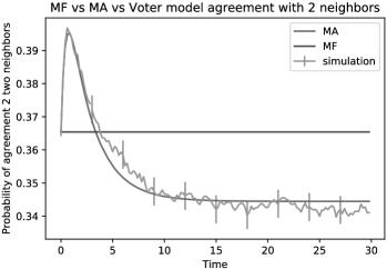
Recall from Figure 2 that for the voter model on the $3$-regular tree $\mathbb{T}_{3}$ (truncated after $9$ generations) the mean-field approximation for the probability of agreement of the root with precisely two of its neighbors was rather inaccurate. Figure 4 plots, for the same tree and parameters, an ad hoc Markovianization of the local equation, wherein $\tilde{\gamma}_{j}$ in (4.15) is replaced with a modified state-dependent version $\bar{\gamma}_{j}:\mathbb{R}_{+}\times\mathcal{X}^{2}\to\mathbb{R}_{+}$ given by

$$\bar{\gamma}_{j}(t,x,y):={\mathbb{E}}[\bar{r}_{j}\bigl{(}t,X_{o}(t),\theta_{o}(t)\bigr{)}\mid(X_{o},X_{1})[t-)=(x,y)[t-)].$$

The good agreement of the simulation with the Markovian version of the local equation in Figure 4 suggests that such a Markovian local equation may serve as a good approximation for several models. This motivates a more rigorous investigation of the accuracty of the Markovian local equation for various classes of models and derivation of rigorous error bounds between the laws of the solution to the Markovianized local equation and the original local equation.

5. Open questions

This article describes the first reduced dimension characterization of marginal dynamics on sparse random graphs, thereby resolving an open question raised in [20] in the context of interacting diffusions. A plethora of open questions remain, related to the structure of the solution to the local equation such as ergodic properties, as well as theoretical guarantees for developing more computationally tractable principled approximations, and also applications (see, for example, [68]). A few open questions are listed below.

5.1. Long-time behavior and invariant measures for the local equations

The results thus far have focused on transient dynamics over finite time intervals. There are several open questions about equilibrium behavior and long-time behavior.

1. Can one can establish general conditions for existence and uniqueness of stationary or invariant measures for the local equation?

2. Can one identify which of these stationary measures correspond to a stationary measure of the evolution on the corresponding infinite graph? Can the local equation be used to identify phase transitions (i.e., identify parameters for existence of multiple stationary distributions on random trees)?

3. Can one study ergodic properties and use the local equation to sample from marginal stationary distributions on random graphs?

Recent work [51, 32] has analyzed some stationarity properties for interacting systems indexed by a regular tree. The work [51] studies limits of systems of diffusions with gradient drift that have an explicit Gibbs measure (i.e., $1$-MRF) as the unique invariant measure on any finite graph, and relates the stationary distribution of the full system to that of a modified local equation. Continuous-state MRFs on infinite trees can also be studied via recursions (see, e.g., [71, 29]). On the other hand, the work [32] studies jump processes with possibly nonreversible dynamics. Also, in [13] the long-time behavior of the Susceptible-Infected-Recovered (SIR) interacting particle system on UGW trees is shown to be succinctly characterized in terms of a fixed point equation.

5.2. Refined convergence results

A natural question is whether one can obtain more refined convergence results, that provide concentration results and rates of convergence, as well as a characterization of fluctuation and large deviations from the hydrodynamic limit. Large deviations principles also provide an alternative way of characterizing hydrodynamic limits.

1. Can one establish large deviation principles and concentration results for interacting particle systems on sparse random graphs?

Such results have been obtained for weakly interacting particle systems on complete and dense graphs (see, e.g., [17, 9, 64, 14, 19, 67, 3]).

5.3. Analytic characterizations

In the mean-field setting, the corresponding nonlinear process and its stationary distribution can also be described by nonlinear PDEs (in the diffusive case) or nonlinear integrodifferential equations (in the jump case).

1. Is it possible to develop a corresponding theory for these new types of path-dependent nonlinear equations that involve conditional laws? Also, can one determine when the marginal laws are absolutely continuous with respect to Lebesgue measure?

5.4. From interacting particle systems to games

Mean-field approximations have been used to study not only interacting particle systems but also games where where strategic agents control their dynamics to maximize an objective function. When the dynamics and objective functions are symmetric, a limit problem called the mean-field game has shown to provide tractable approximations to Nash equilibria in finite-agent games, which are notoriously hard to compute (see [18] for surveys on different aspects of mean-field games).

1. Can one establish limit theorems for Nash equilibria of games with a large number of agents in which the interaction network of agents is sparse rather than the complete graph? While there have been several recent results looking at mean-field games on networks with nodes whose degrees diverge to infinity, there are only a few works studying this on graphs with uniformly bounded degree (see [50] for the study of linear–quadratic games and the works [24, 40, 41] for games on directed graphs).

Acknowledgments. This work was partially supported by the Vannevar Bush Faculty Fellowship ONR-N0014-21-1-2887, Army Research Office grant 911NF2010133 and the National Science Foundation grant DMS-1954351. I would also like to acknowledge several collaborators J. Cocomello, A. Ganguly, D. Lacker, and R. Wu for various joint works on this subject, thank A. Ganguly for generating Figures 1, 2, and 4, and thank J. Cocomello and K. Hu for comments.

References

- [1] D. Aldous and J. Steele, The objective method: probabilistic combinatorial optimization and local weak convergence. In Probability on discrete structures, pp. 1–72, Springer, 2004.
- [2] K. Athreya and P. Ney, Branching processes. Grundlehren Math. Wiss. 196, Springer, 1972.
- [3] R. Baldasso, A. Pereira, and G. Reis, Large deviations for interacting diffusions with path-dependent McKean–Vlasov limit. Ann. Appl. Probab. 32 (2022), no. 1, 665–695. MR 4386539
- [4] V. Barbu and M. Röckner, From nonlinear Fokker–Planck equations to solutions of distribution dependent SDE. Ann. Probab. 48 (2020), no. 4, 1902–1920. MR 4124528
- [5] I. Benjamini and O. Schramm, Recurrence of distributional limits of finite planar graphs. Electron. J. Probab. 6 (2001).
- [6] S. Bhamidi, D. Nam, O. Nguyen, and A. Sly, Survival and extinction of epidemics on random graphs with general degree. Ann. Probab. 49 (2021), no. 1, 1–39.
- [7] P. Biane and R. Durrett, Ten lectures on particle systems. In Lectures on probability theory, edited by P. Bernard, pp. 97–201, Éc. Été Probab. St.-Flour XXIII, Springer, 1993.
- [8] C. Bordenave, Lecture notes on random graphs and probabilistic combinatorial optimization. https://www.math.univ-toulouse.fr/~bordenave/coursRG.pdf, 2016.
- [9] A. Budhiraja, P. Dupuis, and M. Fischer, Large deviation properties of weakly interacting processes via weak convergence methods. Ann. Probab. (2012), 74–102.
- [10] F. Cantelli, Sulla determinazione empirica dellee leggi di probabilità. G. Ist. Ital. Attuari 4 (1933), 421–424.
- [11] P. Cattiaux, S. Roelly, and H. Zessin, Une approche Gibbsienne des diffusions Browniennes infini-dimensionnelles. Probab. Theory Related Fields 104 (1996), 147–179.
- [12] S. Chatterjee and R. Durrett, Contact processes on random graphs with power law degree distributions have critical value 0. Ann. Probab. 37 (2009), no. 6, 2332–2356. MR 2573560
- [13] J. Cocomello and K. Ramanan. Exact description of limiting SIR and SEIR dynamics on locally tree-like graphs. Arxiv Preprint, arXiv:2309.08829 (2023).
- [14] F. Coppini, H. Dietert, and G. Giacomin, A law of large numbers and large deviations for interacting diffusions on Erdős–Rényi graphs. Stoch. Dyn. 20 (2020), no. 2.
- [15] P. Dai Pra and S. Roelly, An existence result for infinite-dimensional Brownian diffusions with non-regular and non-Markovian drift. Markov Process. Related Fields 10 (2004), no. 1, 113–136. MR 2082215
- [16] D. Daley and D. Vere-Jones, An Introduction to the Theory of Point Processes: Volume II: General Theory and Structure. Probability and its Applications. Springer, 2012.
- [17] D. Dawson and J. Gärtner, Large deviations from the McKean–Vlasov limit for weakly interacting diffusions. Stochastics 20 (1987), no. 4, 247–308.
- [18] F. Delarue (ed.), Mean-field games. Proc. Sympos. Appl. Math. 78, American Mathematical Society, 2021.
- [19] F. Delarue, D. Lacker, and K. Ramanan, From the master equation to mean field game limit theory: large deviations and concentration of measure. Ann. Probab. 48 (2020), no. 1, 211–263. MR 4079435
- [20] S. Delattre, G. Giacomin, and E. Luçon, A note on dynamical models on random graphs and Fokker–Planck equations. J. Stat. Phys. 165 (2016), no. 4, 785–798.
- [21] A. Dembo and A. Montanari, Gibbs measures and phase transitions on sparse random graphs. Braz. J. Probab. Stat. 24 (2010), no. 2, 137–211.
- [22] D. Dereudre, Interacting Brownian particles and Gibbs fields on pathspaces. ESAIM Probab. Stat. 7 (2003), 251–277.
- [23] D. Dereudre and S. Rœlly, Path-dependent infinite-dimensional SDE with non-regular drift: an existence result. Ann. Inst. Henri Poincaré Probab. Stat. 53 (2017), no. 2, 641–657. MR 3634268
- [24] N. Detering, J.-P. Fouque, and T. Ichiba, Directed chain stochastic differential equations. Stochastic Process. Appl. 130 (2020), no. 4, 2519–2551.
- [25] J. Deuschel, Infinite-dimensional diffusion processes as Gibbs measures on . Probab. Theory Related Fields 76 (1987), 325–340.
- [26] R. L. Dobrušin, Description of a random field by means of conditional probabilities and conditions for its regularity. Teor. Veroyatn. Primen. 13 (1968), 201–229. MR 0231434
- [27] R. L. Dobrušin, Gibbsian random fields for lattice systems with pairwise interactions. Funktsional. Anal. i Prilozhen. 2 (1968), no. 4, 31–43. MR 0250630
- [28] R. Durret, T. Liggett, F. Spitzer, and A.-S. Sznitman, Interacting particle systems at Saint-Flour. Probab. St.-Flour, Springer, 2012.
- [29] D. Gamarnik and K. Ramanan, Gibbs measures for continuous hardcore models. Ann. Probab. 47 (2019), no. 4, 1949–1981. MR 3980912
- [30] A. Ganguly and K. Ramanan, Hydrodynamic limits of non-Markovian interacting particle systems on sparse graphs. 2022, arXiv:2205.01587v1.
- [31] A. Ganguly and K. Ramanan, Interacting jump processes preserve semi-global Markov random fields. 2022, arXiv:2210.09253v1.
- [32] A. Ganguly and K. Ramanan, Marginal dynamics of interacting particle systems on regular trees: stationarity and Markovian approximations. 2023, Preprint.
- [33] N. Gantert and D. Schmid, The speed of the tagged particle in the exclusion process on Galton–Watson trees. Electron. J. Probab. 25 (2020), 1–27.
- [34] J. Gärtner, On the McKean–Vlasov limit for interacting diffusions. Math. Nachr. 137 (1988), 197–248. MR 968996
- [35] H.-O. Georgii, Gibbs measures and phase transitions. 2nd edn., Stud. Math., De Gruyter, Berlin/New York, 2011.
- [36] V. Glivenko, Sulla determinazione empirica delle leggi di probabilità. G. Ist. Ital. Attuari 4 (1933), 92–99.
- [37] T. E. Harris, Nearest-neighbor Markov interaction processes on multidimensional lattices. Adv. Math. 9 (1972), 66–89.
- [38] T. E. Harris, Contact interactions on a lattice. Ann. Probab. 2 (1974), no. 6, 969–988.
- [39] X. Huang and R. Durrett, The contact process on random graphs and Galton Watson trees. ALEA Lat. Am. J. Probab. Math. Stat. 17 (2020), no. 1, 159–182. MR 4057187
- [40] T. Ichiba, Y. Feng, and J.-P. Fouque, Linear-quadratic stochastic differential games on directed chain networks. J. Math. Stat. Sci. 7 (2021), 25–67.
- [41] T. Ichiba, Y. Feng, and J.-P. Fouque, Linear-quadratic stochastic differential games on random directed networks. J. Math. Stat. Sci. 7 (2021), 79–108.
- [42] C. Kipnis and C. Landim, Scaling limits of interacting particle systems.Grundlehren Math. Wiss. 320, Springer, Berlin, 1999. MR 1707314
- [43] S. Kissel and C. Külske, Dynamical Gibbs–non-Gibbs transitions in lattice Widom–Rowlinson models with hard-core and soft-core interactions. J. Stat. Phys. 178 (2020), no. 3, 725–762.
- [44] A. Kolmogorov, Grundbegriffe der Wahrscheinlichkeitsrchnung. Springer, 1933.
- [45] N. Kolokoltsov, Nonlinear Markov processes and kinetic equations. Cambridge Tracts in Math. 182, Cambridge University Press, 2010.
- [46] C. Külske, Gibbs-Non Gibbs transitions in different geometries: the Widom–Rowlinson model under stochastic spin-flip dynamics. In Statistical mechanics of classical and disordered systems, edited by V. Gayrard, L.-P. Arguin, N. Kistler, and I. Kourkova, pp. 3–19, Springer, 2019.
- [47] D. Lacker, K. Ramanan, and R. Wu, Local weak convergence for sparse networks of interacting processes. Ann. Appl. Probab. 33 (2023), no. 2, 843–888.
- [48] D. Lacker, K. Ramanan, and R. Wu, Locally interacting diffusions as Markov random fields on path space. Stochastic Process. Appl. 140 (2021), 81–114.
- [49] D. Lacker, K. Ramanan, and R. Wu, Marginal dynamics of interacting diffusions on unimodular Galton–Watson trees. Probab. Theor. Related Fields. 187 (2023), 817–884.
- [50] D. Lacker and A. Soret, A case study on stochastic games on large graphs in mean field and sparse regimes. Math. Oper. Res., 48, (2023), 1811–2382.
- [51] D. Lacker and J. Zhang, Stationary solutions and local equations for interacting diffusions on regular trees. Electron. Jour. Probab., (2021).
- [52] O. E. Lanford, III and D. Ruelle, Observables at infinity and states with short range correlations in statistical mechanics. Comm. Math. Phys. 13 (1969), 194–215. MR 256687
- [53] T. Liggett, Interacting particle systems. 1st edn., Springer, New York, 1985.
- [54] T. Liggett, Stochastic interacting systems: contact, voter and exclusion processes. Grundlehren Math. Wiss. 324, Springer, 1999.
- [55] T. M. Liggett, Existence theorems for infinite particle systems. Trans. Amer. Math. Soc. 165 (1972), 471–481. MR 309218
- [56] R. Liptser and A. Shiryaev, Statistics of random processes: I. General theory. 1. Springer, 2001.
- [57] E. Luçon and W. Stannat, Mean field limit for disordered diffusions with singular interactions. Ann. Appl. Probab. 24 (2014), no. 5, 1946–1993. MR 3226169
- [58] H. McKean, Propagation of chaos for a class of non-linear parabolic equations. In Stochastic differential equations, pp. 41–57, Lect. Ser. Differ. Equ., Session 7, Catholic Univ, 1967.
- [59] H. P. McKean, Jr., A class of Markov processes associated with nonlinear parabolic equations. Proc. Natl. Acad. Sci. USA 56 (1966), 1907–1911. MR 221595
- [60] S. Mehri, M. Scheutzow, W. Stannat, and B. Z. Zangeneh, Propagation of chaos for stochastic spatially structured neuronal networks with delay driven by jump diffusions. Ann. Appl. Probab. 30 (2020), no. 1, 175–207. MR 4068309
- [61] R. Minlos, S. Roelly, and H. Zessin, Gibbs states on space-time. Potential Anal. 13 (2000), 367–408.
- [62] D. Nam, O. Nguyen, and A. Sly, Critical value asymptotics for the contact process on random graphs. Transactions of the American Mathematical Society, 375 (2022), 3899-3967.
- [63] K. Oelschlager, A martingale approach to the law of large numbers for weakly interacting stochastic processes. Ann. Probab. (1984), 458–479.
- [64] R. Oliveira and G. Reis, Interacting diffusions on random graphs with diverging degrees: hydrodynamics and large deviations. J. Stat. Phys. 176 (2019),1057–1087.
- [65] R. Oliveira, G. Reis, and L. Stolerman, Interacting diffusions on sparse graphs: hydrodynamics from local weak limits. Electron. J. Probab. 25 (2020), no. 110.
- [66] R. Pemantle, The contact process on trees. Ann. Probab. 20 (1992), no. 4, 2089–2116.
- [67] K. Ramanan, Refined convergence results for interacting diffusions and mean-field games. In Mean-field games, pp. 105–161, Proc. Sympos. Appl. Math. 78, American Mathematical Society, 2021.
- [68] K. Ramanan, Beyond mean-field limits for the analysis of large-scale networks. Queueing Syst. 100 (2022), no. 3–4.
- [69] F. Redig, S. Roelly, and W. Ruszel, Short-time Gibbsianness for infinite-dimensional diffusions with space-time interaction. J. Stat. Phys. 138 (2010), 1124–1144.
- [70] S. Roelly and W. Ruszel, Propagation of Gibbsianness for infinite-dimensional diffusions with space-time interaction. Markov Process. Related Fields 20 (2014), 653–574.
- [71] U. Rozikov, Gibbs measures on Cayley trees. World Scientific, 2013.
- [72] F. Spitzer, Interaction of Markov processes. Adv. Math. 5 (1970), 246–290. MR 268959
- [73] A. Stacey, The contact process on finite homogeneous trees. Probab. Theory Related Fields 121 (2001), no. 4, 551–576. MR 1872428
- [74] A. Sznitman, Topics in propagation of chaos. Springer, 1991.
- [75] P. Tchebichef, Des valeurs moyennes. J. Math. Pures Appl. 2 (1867), no. 12, 177–184.
- [76] A. Van Enter, et al., Possible loss and recovery of Gibbsianness during the stochastic evolution of Gibbs measures. Comm. Math. Phys. 226 (2002), no. 1, 101–130.