Benchmarking of universal qutrit gates

Abstract

We introduce a characterisation scheme for a universal qutrit gate set. Motivated by the rising interest in qutrit systems, we apply our criteria to establish that our hyperdihedral group underpins a scheme to characterise the performance of a qutrit T gate. Our resulting qutrit scheme is feasible, as it requires resources and data analysis techniques similar to resources employed for qutrit Clifford randomised benchmarking. Combining our T gate benchmarking procedure for qutrits with known qutrit Clifford-gate benchmarking enables complete characterisation of a universal qutrit gate set.

I Introduction

Driven by the desire to exploit every precious dimension of Hilbert space that Nature provides [1], the study and development of $d$-level systems (qudits) as extensions to qubits are rapidly developing. Traditional quantum information processing primarily centers on encoding, manipulating, and reading qubits [2]. Qudit experiments are now done using photons [3, 4], trapped ions [5, 6, 7], superconducting qutrits [8, 9, 10], dopants in silicon [11], ultracold atoms [12], and spin systems [13].

For reliable qutrit technology, gate characterization, akin to qubit gates, is crucial [14]. An accepted standard of gate characterisation is randomised benchmarking. rb schemes, in general, are used by experimentalists to estimate the mean average gate fidelity over a set of gates (gate set) [14]. To date, an explicit extension of randomised benchmarking has only been reported for the Clifford gate set [15]. Here, we extend the randomised benchmarking scheme for a universal qutrit gate set.

Qudit applications include quantum teleportation [16, 17], quantum memories [18, 19], Bell-state measurements [20], spin chains [21, 22, 17, 3, 20, 4], and quantum computing [23]. Qutrits offer advantages over qubits such as: superior security for quantum communication [24] or avoiding Hilbert-space truncation of a higher-dimensional system [25].

For quantum computing, a universal gate set is essential to efficiently approximate any gate [2]. Adding a specific gate to the Clifford gate set achieves universality [26, 27]. Such gate is the so-called T gate, which is a non-Clifford member of the third level of the Clifford hierarchy. Interestingly, contextuality presents another avenue for universal quantum computation [27, 28].

Our work is of interest to experimental groups working with a qutrit set of gates. We introduce a RB scheme to characterise a universal set of qutrit gates thereby helping determine the scalability [29] of a qutrit platform. Furthermore, quantum information theorists will find interest in our relaxation of the unitary 2-design condition in a qutrit RB scheme [10].

Our approach extends beyond the qubit case’s geometrical considerations, as detailed in prior studies [30, 31]. In this context, we articulate the prerequisites for an optimal generalisation of dihedral benchmarking. Our findings facilitate the qudit generalization of the dihedral scheme by identifying and broadening the essential features needed by a gate set to characterize T gates effectively.

Whereas methods for characterising arbitrary gate sets are available [32, 33], our work is particularly significant for two reasons. Firstly, we introduce the construction of a gate set that demands minimal resources, specifically necessitating only X and T gates. Secondly, we establish criteria that enable the identification or construction of a gate set capable of characterising a T gate.

Qutrit experiments are proliferating [3, 4, 5, 6, 7, 8, 9, 10, 11, 12, 13], and our extension to experimentally feasible randomised benchmarking schemes for characterising qutrit T gates ushers in full characterisation of universal qutrit gates. Furthermore, our method sets the stage for extending experimental characterisation of a universal set of gates to qutrit cases. With respect to randomised benchmarking theory, our results offer a complete characterisation of the generators of a universal qutrit gate set.

Our work is preceded by the qubit case, wherein characterisation of a T gate is done via dihedral benchmarking [31, 30]. Dihedral benchmarking twirls (i.e., averages over the uniform measure of a group) [34, 14] over a representation of the dihedral group $D_{8}$ [35]. Here, we generalise the dihedral benchmarking (DB) scheme to qutrits. Our scheme is optimal with respect to the number of primitive gates required (X, T, and H); we use upright letters for gates and slanted font for the corresponding matrices.

We now start the discussion of our extension of dihedral benchmarking to qutrit systems. We justify our focus on qutrits as currently there is an increasingly number of qutrit implementations [3, 4, 5, 6, 7, 8, 9, 10, 11, 12, 13]. Furthermore, in the qutrit case, we know that our generalisation of $D_{8}$ (and the corresponding irreducible representation (irrep)) is the unique pair leading to an optimal generalisation of dihedral benchmarking. Before establishing our qutrit generalisation of the dihedral group, we first recall several key mathematical concepts in randomised benchmarking schemes for qutrits.

II Background

We introduce part of the key algebraic entities needed in our work. We work in the three-dimensional Hilbert space $\mathscr{H}\coloneqq\mathrm{span}(\ket{0},\ket{1},\ket{2})$. A state $\rho$ is a positive trace-class operator with trace 1 [36]. The set of states in $\mathscr{H}$ is denoted $\mathscr{D}$; pure states are the extreme points of $\mathscr{D}$ and are of the form

$$\rho_{\psi}\coloneqq\outerproduct{\psi}{\psi},\quad\ket{\psi}\in\mathscr{H}.$$ (1)

Then for a mapping $\mathcal{E}\colon\mathscr{D}\to\mathscr{D}$ and $\ket{\Omega}\coloneqq\nicefrac{{1}}{{\sqrt{3}}}(\ket{00}+\ket{11}+\ket{22})$, the Choi-Jamiołkowski operator is $\mathscr{J}_{\mathcal{E}}\coloneqq 3(\mathcal{E}\otimes\mathbb{I})\left(\outerproduct{\Omega}{\Omega}\right)$.

We now describe the representation of the algebraic objects introduced in the previous paragraph. We denote by $\Lambda_{\mathcal{E}}$ the matrix representation (in the computational basis of $\mathscr{H}^{\otimes 2}$) of $\mathscr{J}_{\mathcal{E}}$. States $\{\rho\}$ are represented by a nine-dimensional vector $|\rho\rangle\!\rangle$ satisfying $|\mathcal{E}(\rho)\rangle\!\rangle=\Lambda_{\mathcal{E}}|\rho\rangle\!\rangle$; $|\rho\rangle\!\rangle$ is computed by stacking the rows of the matrix representation (in the computational basis) of $\rho$ [37, 38]. We emphasise gates are physical objects; therefore, it is incorrect to discuss their representation.

The qutrit T gate has an important role within quantum computing. A T gate correspond to the action of some unitary matrix $T\in\mathcal{C}_{3}\setminus\mathcal{C}_{2}$ [1, 39, 40], with $\mathcal{C}_{l}$ the $l$th level of the qutrit Clifford hierarchy. For convenience, we only consider diagonal $T$ matrices. Let $\omega_{d}\coloneqq\exp(2\pi\mathrm{i}/d)$. For qutrits, the generalised Hadamard and a T matrix are [41]

$$H \coloneqq\nicefrac{{1}}{{\sqrt{3}}}\begin{bmatrix}1&1&1\\ 1&\omega_{3}&\omega_{3}^{2}\\ 1&\omega_{3}^{2}&\omega_{3}\end{bmatrix},\,T\coloneqq\matrixquantity[1&&\\ &\omega_{9}^{8}&\\ &&\omega_{9}],$$ (2)

respectively. The gates generated by H and T, denoted by the generating set $\langle\mathrm{H},\mathrm{T}\rangle$, is a universal gate set [39, 40, 42]. The corresponding set of matrices is denoted by $\langle H,T\rangle$.

The qutrit Pauli group is defined in terms of the Heisenberg-Weyl (HW) matrices, themselves one natural unitary generalisation of the Pauli matrices [43]. The qutrit HW matrices are powers of the clock and shift matrices [44, 45]:

$$Z\ket{i}\coloneqq\omega_{3}^{i}\ket{i},X\ket{i}\coloneqq\ket{i\oplus 1},i\in[3]\coloneqq\{0,1,2\},$$ (3)

with $\oplus$ denoting addition modulo 3 and $[k]\coloneqq\{0,\ldots,k-1\}$. In turn, the HW matrices $\{W_{k},k\in[9]\}$ correspond to $W_{3i+j}\coloneqq X^{i}Z^{j},\text{for }i,j\in[3]$: $\mathcal{W}\coloneqq\{W_{3i+j}\colon i,j\in[3]\}$. Then the qutrit Pauli group is $\mathcal{P}\coloneqq\langle\mathcal{W},\omega_{3}\mathbb{I}\rangle$.

Several concepts from representation theory are used in our work [46]. Given a finite group $\mathbb{G}$ and a vector space $\mathscr{V}$, a representation $\sigma$ is a homomorphic mapping from $\mathbb{G}$ to $\operatorname{GL}(\mathscr{V})$; henceforth $\mathscr{V}$ refer to either $\mathscr{H}$ or $\mathscr{H}^{\otimes 2}$. For concreteness, we employ the canonical isomorphisms $\operatorname{GL}(\mathscr{H})\cong\mathscr{M}$ and $\operatorname{GL}(\mathscr{H}^{\otimes 2})\cong\mathscr{M}^{\otimes 2}$, to ensure our representations are matrices. The range (or image) of $\sigma$ is denoted $\operatorname{Ran}(\sigma)\coloneqq\{\sigma(g)\colon g\in\mathbb{G}\}$.

The term irreducible representation can refer to a subspace and to a mapping. Given a non-trivial subspace $\Sigma\subseteq\mathscr{V}$ invariant under the action of $\sigma$, we decompose $\mathscr{V}=\Sigma\oplus\Sigma^{\perp}$, where ^⟂ denotes orthogonal complement. In general, if $\sigma$ has an ordered multiset of non-trivial invariant subspaces $\{\Sigma_{i}\}$, $\mathscr{V}$ can be decomposed as

$$\mathscr{V}=\bigoplus_{i}\Sigma_{i}.$$ (4)

The subspaces {$\Sigma_{i}$} are known as irreps, mostly in the context of the decomposition of a representation in irreps [46]. Unless specified, capital Greek letters represent irreps as subspaces, whereas lowercase Greek letters indicate their homomorphic mappings.

We now introduce the representation of a group computed from the Choi matrix. Let $\mathbb{G}$ be a finite group with a unitary representation $\sigma\colon\mathbb{G}\to\mathscr{M}$. We define the representation $\Lambda_{\sigma}\colon\mathbb{G}\to\mathscr{M}^{\otimes 2}$ that maps $g\in\mathbb{G}$ to $\Lambda_{\sigma}(g)\coloneqq\sigma(g)\otimes\sigma(g)^{*}$, where ^∗ denotes complex conjugation. We refer to $\Lambda_{\sigma}(g)$ as a gate. We sometimes shorten $\Lambda_{\sigma}(g)$ by $\Lambda_{g}$ when the knowledge of $\sigma$ is implicit or unnecessary; we follow the convention of using a Greek subindex to denote the representation and a Latin subindex an element of such representation.

We recall the definition of the twirl by a representation of a group. Let $\mathbb{G}$ be a finite group with a three-dimensional representation $\sigma$. The twirl of a channel $\mathcal{E}$ over a group $\mathbb{G}$ is

$$\mathcal{T}_{\mathcal{E}}^{(\mathbb{G},\sigma)}\coloneqq\underset{g\in\mathbb{G}}{\mathbb{E}}\Lambda_{g}^{\dagger}\Lambda_{\mathcal{E}}\Lambda_{g},$$ (5)

where $\mathbb{E}_{x\in\mathbb{X}}$ denotes average over the uniform measure on $\mathbb{X}$; that is, $x$ has probability $1/|\mathbb{X}|$. We generally omit the pair group-irrep $(\mathbb{G},\sigma)$ in writing the left-hand side of Eq. (5); the trace of $\mathcal{T}_{\mathcal{E}}$ is used in RB schemes to estimate the average gate fidelity (AGF).

Before passing to the next section, we define the ideal and noisy versions of a channel labelled by a group element. Let $g\in\mathbb{G}$, we call $\Lambda_{g}$ the ideal channel corresponding to $g$. Then if $\mathcal{E}_{g}$ is a channel associated with the noise accompanying the action of the gate $\Lambda_{g}$, the noisy version of $\Lambda_{g}$ is

$$\tilde{\Lambda}_{g}\coloneqq\Lambda_{\mathcal{E}_{g}}\Lambda_{g}.$$ (6)

Using the tools of representation theory and quantum channels presented above, we then formulate our generalisation of DB.

III Approach

We are now ready to describe our approach to articulating and solving the problem of benchmarking a universal set of qutrit gates. First we introduce the HDG as a generalisation of the dihedral group, needed for generalising qubits to qutrits. Then we elaborate on our benchmarking scheme for the HDG. We discuss the formal properties our scheme generalises from the qubit case.

III.1 Hyperdihedral group

We now introduce our generalisation of $D_{8}$, which we call hyperdihedral group (HDG). Our extension of DB is based on a unitary irreducible representation (unirrep) of the HDG. We establish this representation in the following two paragraphs. The HDG is the semidirect product, we formally specify the product later, between $C_{3}$ and $C_{9}^{\times 2}$. We justify the choice of the HDG in Appendix §C.1. We discuss the characterisation of other diagonal gates at the end of this subsection.

The unirrep for HDG is defined using two auxiliary representations. The first auxiliary representation is $\repX\colon C_{3}\to\mathscr{M}$. If the abstract elements of the order-three cyclic group $C_{3}$ are $\{a^{k}\colon k\in[3]\}$, the mapping $\repX$ is $\repX{a^{k}}=X^{k}$, where $X$ is given in Eq. (3).

The second auxiliary representation is now introduced and used to define the unirrep we use for the HDG. Consider the mapping $\repC\colon C_{9}^{\times 2}\to\mathscr{M}$. If the elements of $C_{9}^{\times 2}$ are $\bm{\alpha}=(\alpha_{0},\alpha_{1})\in[9]^{\times 2}$, then $\repC{\bm{\alpha}}=T^{\alpha_{0}}(T^{\prime})^{\alpha_{1}}$, where $T^{\prime}\coloneqq\operatorname{diag}[\omega_{9}^{2},\omega_{9}^{6},\omega_{9}]$. Using $\repX$ and $\repC$, the HDG irrep our scheme uses is

$$\gamma\colon\mathrm{HDG}\to\mathscr{M}\colon(a^{k},\bm{\alpha})\mapsto\repX(a^{k})\repC{\bm{\alpha}}.$$ (7)

Notice $\operatorname{Ran}(\gamma)=\langle T,X\rangle$, which is reminiscent of $D_{8}$.

We now provide the definition of the HDG. Consider the automorphism $\phi\in\operatorname{Aut}(C_{9}^{\times 2})$ is

$$\phi(T)\coloneqq T^{3}(T^{\prime})^{4},\quad\phi(T^{\prime})\coloneqq T^{8}(T^{\prime})^{5}.$$ (8)

Considering $\phi$, the HDG is completely defined by

$$\mathrm{HDG}\coloneqq C_{3}\ltimes_{\phi}C_{9}^{\times 2};$$ (9)

the mapping $\phi$ depends on $T$. Additional details can be found in Appendix B.

We discuss several properties of the HDG and the resulting RB scheme. The HDG, consisting of 243 group elements, requires only 81 gates when global phases are removed [10]. Consequently, our scheme uses fewer gates than Clifford-based RB schemes. It is worth mentioning that $H\not\in\operatorname{Ran}(\gamma)$, which is a property shared with DB.

Our scheme has another two additional characteristics useful in practical settings. The entire set of HDG gates is generated solely by the X and T gates, which also enjoy a simplified multiplication rule between group elements. The AGF and survival probability (SP), derived from averaging over the HDG, are dependent on two complex parameters.

The HDG is a natural generalization of $D_{8}$; like $D_{8}$, it has a semidirect product structure [47]. As a result of the semidirect product structure of the HDG, group elements and their products can be straightforwardly expressed as powers of the generating elements, as done in Appendix B. Thus, sampling from the HDG is straightforward and does not require approximate methods, as is generally necessary for arbitrary finite groups [48].

We now discuss the prerequisites of our scheme. Our scheme requires three primitive gates (X, T, and H), state preparation and measurement (SPAM) of $\ket{0}$ and $\ket{+}\coloneqq H\ket{0}$, and the construction of circuits with a depth of up to 200 HDG gates. Among these gates, the X and T gates are the generators of the benchmarked gate set, whereas the H gate is only required to prepare the state $\ket{+}$.

Current qutrit experiments satisfy the requirements of our scheme [9, 10]. For instance, the Berkeley implementation (BI) [10] uses primitive gates for rotations in the subspaces $\operatorname{span}(\ket{0},\ket{1})$ and $\operatorname{span}(\ket{1},\ket{2})$. These authors have also reported the composition of more than 200 qutrit gates. These characteristics support the claim that our scheme is currently feasible.

Our scheme is not limited to the characterisation of $T$ in Eq. (2). By substituting $T$ by any other diagonal matrix (in the computational basis) with order at least three, the construction of the HDG can be applied to such gate. The resulting representation has the same irrep decomposition as the HDG. Thus, our scheme is useful to characterise any diagonal gate with order at least three.

We chose to employ the T gate, as defined in Eq. (2), for it enables universal quantum computing. Using non-Clifford gates like $T$ is beneficial due to the availability of established magic-state distillation procedures for generating such a gate. Furthermore, the use of magic-state distillation is notably advantageous, as this method has been integrated into error-correcting codes [49].

IV Results

We now provide the expressions for the AGF and the SP resulting from using a HDG gate set. These expressions correspond to our genersalisation to qutrits of dihedral benchmarking. We also show our scheme is made, as Clifford RB schemes are, SPAM-error independent by adding a projector to the SP expression.

IV.1 Survival probability and average gate fidelity

We introduce our scheme to characterise a universal gate set, which is our generalisation for qutrits of DB. Our scheme feasibly estimates the AGF of the HDG gate set. Our analysis assumes every gate-set member has the same noise, which is referred to as gate-independent analysis. It is worth mentioning that our scheme is compatible with the Fourier transform method [50, 51]. We introduce our scheme first by presenting the twirl computed over the HDG and then the expressions for the AGF and the SP.

We now write the explicit expression of the twirl. We start by considering the projectors onto the different representation spaces [46] in Eq. (37) of Appendix C: $\Pi_{\mathbb{I}},\Pi_{\Gamma_{0}},\Pi_{\Gamma_{0}^{*}},\Pi_{\Gamma_{+}},\Pi_{\Gamma_{+}^{*}}.$ The eigenvalues are

$$\lambda_{\Gamma}(\mathcal{E})\coloneqq\frac{\tr(\Lambda_{\mathcal{E}}\Pi_{\Gamma})}{\tr(\Pi_{\Gamma}\Pi_{\Gamma}^{\top})}.$$ (10)

Then the twirl of a channel $\mathcal{E}$ over the HDG is

$$\mathcal{T}_{\mathcal{E}}=\sum_{\Gamma\in\{\Gamma_{\mathbb{I}},\Gamma_{0},\Gamma_{0}^{*},\Gamma_{+},\Gamma_{+}^{*}\}}\lambda_{\Gamma}(\mathcal{E})\Pi_{\Gamma}.$$ (11)

From Eq. (11), there are only two non-trivial complex entries: $\lambda_{0}$ and $\lambda_{+}$. Let $\varsigma\in\{0,+\}$, then the parameters $\lambda_{\varsigma}$ are conveniently written in polar form:

$$\lambda_{\varsigma}=r_{\varsigma}\exp(\mathrm{i}\varphi_{\varsigma}).$$ (12)

We now write the SP in our scheme. The gate-independent conditions means that for all group members $g\in\mathrm{HDG}$, the noisy channel has the form

$$\tilde{\Lambda}_{g}=\Lambda_{\mathcal{E}}\Lambda_{g};$$ (13)

that is, every gate set member has the same noise channel $\mathcal{E}$. Let $\rho$ be a state, $E\in\{\rho,\mathbb{I}-\rho\}$, and $m$ a positive integer. Using the assumption of Eq. (13), the SP for the HDG is

$$\Pr(m;\rho,E,\mathrm{HDG})=\langle\!\langle E|\Lambda_{\mathcal{E}}\mathcal{T}_{\mathcal{E}}^{m}|\rho\rangle\!\rangle.$$ (14)

We rewrite Eq. (14) knowing $\mathcal{T}_{\mathcal{E}}$ is diagonal to obtain:

$$\Pr(m;\rho,E,\mathrm{HDG})=\sum_{\Gamma}\lambda_{\Gamma}^{m}(\mathcal{E})\langle\!\langle E|\Lambda_{\mathcal{E}}\Pi_{\Gamma}|\rho\rangle\!\rangle,$$ (15)

where the sum is over the irreps in the decomposition of Eq. (37).

We now show how Eq. (15) is used to estimate, from the circuit depth vs SP curve, the AGF over HDG. We obtain the expression for the SP curve, which is a decaying exponential function. To express the SP as a function of the twirl entries, we consider the states

$$\rho_{\varsigma}\coloneqq\outerproduct{\varsigma}{\varsigma},\quad\varsigma\in\{0,+\}.$$ (16)

Substituting $\rho$ in Eq. (15) with $\rho_{\varsigma}$ given in Eq. (16) we obtain the SP

$$\Pr(m;\rho_{\varsigma},\rho_{\varsigma},\mathrm{HDG})=\frac{1}{3}+\frac{2}{3}b_{\varsigma}r_{\varsigma}^{m}\cos(m\varphi_{\varsigma}).$$ (17)

Thus, the SP can be used to estimate the AGF.

At this point we now introduce the AGF and relate it to the SPs written in Eqs. (17). The AGF computed over a group $\mathbb{G}$ is defined as:

$$\bar{\operatorname{F}}\coloneqq\underset{g\in G}{\mathbb{E}}\operatorname{F}(\tilde{\Lambda}_{g},\Lambda_{g}),$$ (18)

where $\operatorname{F}(\tilde{\Lambda}_{g},\Lambda_{g})$ is the gate fidelity between the ideal and the noisy channel corresponding to $\Lambda_{\sigma}(g)$. In general, for any pair of qutrit channels $\cal E$ and $\mathcal{E}^{\prime}$, the AGF $\operatorname{F}(\mathcal{E}^{\prime},\cal E)$ is [52]

$$\operatorname{F}({\mathcal{E}^{\prime}},{\cal E})\coloneqq\frac{1}{12}\tr{\Lambda_{\mathcal{E}^{\prime}}^{\dagger}\Lambda_{\mathcal{E}}}+\frac{1}{4}.$$ (19)

Next, we write the AGF in terms of the twirl parameters. For gate-independent benchmarking, the quantity estimated by HDG benchmarking [30] is the AGF between the twirl and the identity

$$\bar{\operatorname{F}}=\operatorname{F}(\mathcal{T}_{\mathcal{E}},\mathbb{I})=\frac{1}{12}\tr\mathcal{T}_{\mathcal{E}}+\frac{1}{4},$$ (20)

where $\mathcal{T}_{\mathcal{E}}$ is defined in Eq. (5). For the qutrit HDG, using Eqs. (17):

$$\bar{\operatorname{F}}=\operatorname{F}(\mathcal{T},\mathbb{I})\\ =\frac{1}{12}(1+2r_{0}\cos\varphi_{0}+6r_{+}\cos\varphi_{+})+\frac{1}{4}.$$ (21)

Note how the quantities $b_{\varsigma}$ in Eq. (17) are not needed to estimate the AGF.

It is possible to neglect the phases in Eq. (21): we justify in Appendix A that for high-fidelity configurations $\varphi_{0}\ll 1$ and $\varphi_{+}\ll 1$. Thus, we simplify Eq. (21) to

$$\bar{\operatorname{F}}=\operatorname{F}(\mathcal{T},\mathbb{I})\approx\frac{1}{12}(1+2r_{0}+6r_{+})+\frac{1}{4}.$$ (22)

Notice that the previous approximation for the AGF is always valid. However, for large values of $m$, the single exponential approximation for the SP could fail; we study the validity of the single-exponential approximation in Appendix A.

IV.2 Removal of SPAM-error contributions

An important feature of Clifford randomised benchmarking schemes is their independence of SPAM errors [53]. However, the HDG SP given in Eq. (17) is not SPAM error-free (SEF). One way to overcome this limitation is by computing a projector [48] that, when multiplied with the twirl, leads to an expression of the survival probability with a single parameter; thus our scheme is SEF.

The projector-based method for term removal is not the only option and may sometimes be superfluous. There are known alternatives to this approach [54, 55]. Furthermore, if a gate set achieves a fidelity of approximately $\bar{\operatorname{F}}\approx 0.99$, the need for SPAM removal techniques diminishes, as illustrated in §V and explored in other studies [32].

We now compute the projectors. The Choi matrix of the X and Z gates satisfies

$$\mathbb{P}_{\varsigma}\coloneqq\sum_{k\in[3]}\Lambda_{Q_{\varsigma}^{k}},$$ (23)

where $\varsigma\in\{0,+\}$, $Q_{0}\coloneqq X$, $Q_{+}\coloneqq Z$. The projectors $\mathbb{P}_{\varsigma}$ satisfy: $\mathbb{P}_{+}\Pi_{\Gamma_{0}}=\mathbb{P}_{+}\Pi_{\Gamma_{0}^{*}}=\mathbf{0}$ and $\mathbb{P}_{0}\Pi_{\Gamma_{+}}=\mathbb{P}_{0}\Pi_{\Gamma_{+}^{*}}=\mathbf{0}$, where $\mathbf{0}$ is the null matrix in $\mathscr{M}^{\otimes 2}$.

By multiplying $\mathcal{T}_{\mathcal{E}}$ from the left by $\mathbb{P}_{\varsigma}$ we remove every parameter in Eq. (11) except $\lambda_{\varsigma}$ . Therefore, using a modified SP—with powers of the clock and shift matrices—we can obtain a SP which depends only on selected parameters, independently of the initial state and the final measurement. We compute such SP in the next paragraph.

The modified SP—by which we mean including the projectors in Eq. (23)—is

$$\check{\Pr}(m;\rho,E,\mathrm{HDG};\varsigma,k)\coloneqq\langle\!\langle E|\Lambda_{Q^{k}_{\varsigma}}\Lambda_{\mathcal{E}}\mathcal{T}_{\mathcal{E}}^{m}|\rho\rangle\!\rangle,$$ (24)

where $k\in[3]$. Using Eq. (24), we reach the SEF version of the SPs (17):

$${\Pr}_{\varsigma}^{\rm SEF}\coloneqq\sum_{k\in[3]}\check{\Pr}(m;\rho,E,\mathrm{HDG};\varsigma,k)=\lambda_{\mathbb{I}}+2\Re{(\lambda_{\varsigma}^{m}\alpha_{\varsigma}^{\text{SEF}})},$$ (25)

where $\alpha_{\varsigma}^{\mathrm{SEF}}\in\mathbb{C}$ are constants absorbing SPAM contributions. Eq. (25) shows that, even if the coefficients depend on the initial state preparation, the eigenvalues $\lambda_{\varsigma}$ remain unchanged so that the expression of $\bar{\operatorname{F}}$ in Eq. (18) is SEF.

V Numerics

In this section we numerically investigate the feasibility of our scheme. Our study is done by comparing the variance of the Clifford and HDG gate sets. This is done using experimental resources reported for a transmon qutrit [10]. Our results show that both variances are qualitatively similar. Thus, given that the experimental resources required for our scheme are similar to those of Clifford RB, if Clifford RB can be implemented, our scheme can likewise be appropriately executed.

V.1 Noise model

We introduce examples of channels used to add noise to HDG gates. These channels are motivated by the features of the BI and the noise models presented elsewhere [51].

In determining the appropriate noise for each gate, we observe the following distinction: elements within the HDG fall into two distinct categories—diagonal matrices and powers of $X$. Notably, the $X$ gates’ implementation differs from that of the diagonal gates [22]. Given this difference, we introduce specific noise types for each: for the diagonal matrices, we incorporate noise by adding a phase to the state $\ket{1}$, whereas for the powers of $X$, we introduce an over-rotation error.

In our example, the over-rotation error corresponds to adding a phase to the state $\ket{1}$. Thus we represent this noise by conjugating a state by the following unitary matrix:

$$U_{\varphi}\coloneqq\begin{bmatrix}1&&\\ &\exp(\mathrm{i}\varphi)&\\ &&1\end{bmatrix}.$$ (26)

For the over-rotation error, the mapping corresponds to the conjugation of an state by a matrix of the form

$$U_{(\psi,\xi)}\coloneqq V\exp(-\mathrm{i}\psi M_{01})\exp(-\mathrm{i}\xi M_{12})V^{\dagger},$$ (27)

where $\psi,\xi\in[0,2\pi)$, $V\sim\mathsf{Haar}({\rm SU}(3))$ is a matrix randomly sampled using the ${\rm SU}(3)$ Haar measure [56], and

$$M_{01}\coloneqq\begin{bmatrix}1&&\\ &-1&\\ &&1\end{bmatrix},\quad M_{12}\coloneqq\begin{bmatrix}1&&\\ &1&\\ &&-1\end{bmatrix}.$$ (28)

V.2 Survival probability statistics

We now analyse numerically the SP. The primary objective of this examination is to highlight the similarities between the variances of the Clifford and HDG gate sets. Notably, similar variance behaviours suggest a similar number of samples required across both methods. Given our reliance on a small subset of the Clifford gate set, excluding $T$, the feasibility of our scheme is related to this sample count.

Through a numerical analysis, we determine the variance of the HDG SP when subjected to noise. This is important, as the determination of the number of samples required depends on the variance. Although there is a model for the variance [57], it includes numerous parameters; these parameters limit its practicality.

Alternatively, a two-parameter empirical model is stated for qubit Clifford randomised benchmarking (RB) [58]. Unfortunately, this latter model asymptotically approaches zero. This behaviour is not seen in qutrits, where the variance converges to a non-zero value.

The variance of the SP is

$$\operatorname{V}(m;\rho,E,\mathbb{G})\coloneqq\langle\!\langle E^{\otimes 2}|\Lambda_{\mathcal{E}}^{\otimes 2}(\mathcal{T}_{\mathcal{E}^{\otimes 2}})^{m}|\rho^{\otimes 2}\rangle\!\rangle\\ -\langle\!\langle E^{\otimes 2}|\Lambda_{\mathcal{E}}^{\otimes 2}(\mathcal{T}^{\otimes 2}_{\mathcal{E}})^{m}|\rho^{\otimes 2}\rangle\!\rangle,$$ (29)

where $m$ is the circuit depth, $\mathcal{T}_{\mathcal{E}^{\otimes 2}}\coloneqq\mathbb{E}_{g}\Lambda_{g}^{\otimes 2}\Lambda_{\mathcal{E}}^{\otimes 2}(\Lambda_{g}^{\otimes 2})^{\dagger}$, $\rho$ is the initial state, and $E$ the final measurement [57]. An example of the variance of the SP (for qutrit Clifford and HDG) is presented in Fig. 1.

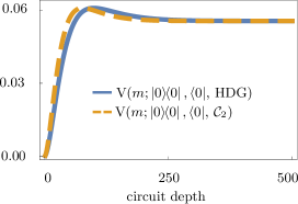
Figure 1: This figure shows the variance for two SPs, differentiated by the gate set used in the simulation: blue and orange lines correspond to the HDG and Clifford gate sets, respectively; the variable $m$ in the argument of $\mathrm{V}$ denotes the circuit depth. We observe that the two curves are qualitatively similar. In the plot we present the variance for the SP for a configuration with $\operatorname{F}(\Lambda_{U_{\varphi}})=0.9999$ and $\operatorname{F}(\Lambda_{(\psi,\psi)})=0.99$ (in Eqs. (26) and (27)), using $\ket{0}$ as initial state.

These numerical results show that the variance of the SP for the HDG gate set is qualitatively similar to the Clifford case. Consequently, it is reasonable to expect that the number of required samples should be comparable.

VI Discussion

Our extension of the randomised benchmarking scheme to characterise T gates is given by the expressions  (17) and (25), together with the qutrit HDG gate sets. To summarise our steps, we obtained the expression for the HDG AGF in Eq. (22). We then showed that the parameters of the HDG AGF are accessible via fit from the survival probabilities in Eqs. (17) and Eqs. (25) respectively for ideal and noisy—subject to SPAM errors—initial states.

Next we examined the experimental resources required for our scheme. Compared with the 216 gates of the Clifford group, the 81 gates of the quotient HDG/$\langle\omega_{3}\mathbb{I}\rangle$ reduce by $\sim 2/3$ the number of gates required for benchmarking and provide a more efficient scheme than interleaved benchmarking, with respect to the gates needed to be synthesised [14].

We then analysed the practical properties of our scheme. By enforcing the condition of a diagonal twirl, we simplified the data analysis required for computing the AGF. This is especially clear compared to the non-diagonal cases [48, 33]. Additionally, the semidirect product structure of the HDG allows the efficient sampling of HDG elements, eliminating the need for approximate Markov chain methods [48]. Finally, we asserted our scheme is feasible as it is based on gates (X, H, and T) that can be implemented by current platforms [10, 9].

In §V, we simulated our scheme using the experimental parameters from a transmon qutrit [10]. Our findings indicate that the statistics of the HDG SP closely resemble those of the Clifford gate set [57]. Consequently, comparable experimental resources—such as measurements and the number of randomly sampled circuits—are required, and the same statistical tools can be employed.

We conclude our discussion with a comment on non-Clifford interleaved benchmarking [30, 14]. The HDG can be used to characterise diagonal gates. However, our schemes and the construction of the HDG, cannot be used to characterise the X gate. The reason is that, by removing the X gate from the HDG, we obtain an abelian subgroup. Twirling by an abelian group leads to a twirl with more parameters than for the HDG [59].

VII Conclusions

We have extended the randomised benchmarking scheme to characterise qutrit T gates. Our scheme relies on our generalisation of the dihedral group for qubits, which we call the hyperdihedral group. Using the hyperdihedral group, we derived closed-form expressions for the survival probability and average gate fidelity for gate sets that include a qutrit T gate. Our scheme characterises a diagonal qutrit T gate, the non-Clifford generator of a universal qutrit gate set. Thus, our extension completes the characterisation of a universal qutrit gate set. Finally, to prove our scheme’s feasibility, we simulated its application on a transmon qutrit T gate [10].

DAA, BCS, and HdG acknowledge support from Natural Sciences and Engineering Research Council of Canada and the Government of Alberta.

Appendix A Effect of phases on the survival probability and average gate fidelity

In this section, we study the effect of the phases in Eq. (12) on the survival probability curve and average gate fidelity. We show that, for high-fidelity gates, the contribution of the phases can be neglected in the AGF. However, for high-depth circuits, the survival probability curve deviates from a single exponential.

To consider the most general case, we express the phase in terms of the $\chi$-representation. This representation has its origins in quantum tomography [2, 60]. We use this representation to obtain the general expression for the phase in eigenvalue $\lambda_{0}$ in Eq. (12). In the $\chi$-representation, the phase in Eq. (12) is given by

$$\varphi_{0}=2\arctan\left(\frac{v}{\sqrt{u^{2}+v^{2}}+u}\right),$$ (30)

where $u\coloneqq\real(\lambda_{0})$, and $v\coloneqq\imaginary(\lambda_{0})$. Specifically, we have

$$u =\chi_{00}+\chi_{11}+\chi_{22}$$ (31a)

$$-\frac{1}{2}(\chi_{33}+\chi_{44}+\chi_{55}+\chi_{66}+\chi_{77}+\chi_{88}),$$

$$v =\frac{2}{\sqrt{3}}\left(\chi_{33}+\chi_{44}+\chi_{55}-\chi_{66}-\chi_{77}-\chi_{88}\right).$$ (31b)

We now analyse the asymptotic behaviour of the phase for high-fidelity gates. High-fidelity implies $\chi_{00}\lessapprox 1$ and $\chi_{ii}\ll 1$ for $i>0$. This implies that $u\approx 1$ and $v\ll 1$. Asymptotic behaviour of $\cos\varphi_{0}$ is

$$\cos\varphi_{0}=1-\frac{1}{2}\left(\frac{v}{u}\right)^{2}+\mathcal{O}((u/v)^{4})\\ \approx 1-\frac{1}{2}\left(\frac{1-\bar{\operatorname{F}}}{\bar{\operatorname{F}}}\right)^{2}.$$ (32)

Eq. (32) shows that for high-fidelity gates approximation Eq. (22) is valid.

However, the experimental estimate of the eigenvalues $\lambda_{\varsigma}$ could be affected by the phase in Eq. (12). We study the case when the phase $\varphi_{0}$ is maximal for a given AGF. We consider $\bar{\operatorname{F}}=0.9925$. In Fig. 2 we show the logarithm of the SP. From Fig. 2 we notice a deviation from a straight line; this deviation indicates the SP is not a single-exponential. The shape of this curve makes it difficult to estimate the parameter if the number of composed gates is large.

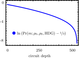
Figure 2: Log plot of the SP $\Pr$ of Eq. (17) for a gate-independent RB run. The noise was fixed with $\bar{\operatorname{F}}=0.9925$. We highlight the presence of the oscillatory contribution as a deviation from a straight line.

The contribution of the phase to the SP in Eq. (17) is assessed by an asymptotic expansion. For large values of the fidelity

$$\cos m\varphi_{0}=1-\frac{1}{2}(mu/v)^{2}+\mathcal{O}((u/v)^{4})\\ \approx 1-\frac{1}{2}(m(1-\bar{\operatorname{F}})/\bar{\operatorname{F}})^{2}.$$ (33)

Therefore, even for high-fidelity gates, shallower circuit depths must be considered for the single-exponential fit. Otherwise the presence of the phase produces a bad fit.

Appendix B Constructing and manipulating qutrit HDG elements

For convenience, we construct elements in the qutrit HDG by computing products of the matrices $X$, $A_{1}\coloneqq\operatorname{diag}[1,\omega_{9}^{8},\omega_{9}]$, and $A_{2}\coloneqq\operatorname{diag}[\omega_{9}^{2},\omega_{9}^{6},\omega_{9}]$, where $\omega_{9}\coloneqq\exp(2\pi i/9)$. Each HDG member $X^{x}A_{1}^{y}A_{2}^{z}$ is labelled by the $(x,y,z)$, where $x,y\in\mathbb{Z}_{3}$, $z\in\mathbb{Z}_{9}$. For two words $(x_{1},y_{1},z_{1})$ and $(x_{2},y_{2},z_{2})$ labelling HDG elements $X^{x_{1}}A_{1}^{y_{1}}A_{2}^{z_{1}}$ and $X^{x_{2}}A_{1}^{y_{2}}A_{2}^{z_{2}}$ respectively, the resulting group element is $X^{x_{3}}A_{1}^{y_{3}}A_{2}^{z_{3}}=X^{x_{1}}A_{1}^{y_{1}}A_{2}^{z_{1}}X^{x_{2}}A_{1}^{y_{2}}A_{2}^{z_{2}}$ where $(x_{3},y_{3},z_{3})$ is given by

$$\begin{bmatrix}x_{3}\\ y_{3}\\ z_{3}\end{bmatrix}\coloneqq\begin{bmatrix}1&0&0\\ 0&5&8\\ 0&4&3\end{bmatrix}^{x_{2}}\begin{bmatrix}x_{1}\\ y_{1}\\ z_{1}\end{bmatrix}+\begin{bmatrix}x_{2}\\ y_{2}\\ z_{2}\end{bmatrix}.$$ (34)

Similarly, for an HDG element $(x_{1},y_{1},z_{1})$, the inverse word $(x_{2},y_{2},z_{2})$ satisfying

$$(X^{x_{1}}A_{1}^{y_{1}}A_{2}^{z_{1}})(X^{x_{2}}A_{1}^{y_{2}}A_{2}^{z_{2}})=\mathbb{I}_{3}$$ (35)

is given by

$$\begin{bmatrix}x_{2}\\ y_{2}\\ z_{2}\end{bmatrix}\coloneqq-\begin{bmatrix}1&0&0\\ 0&5&8\\ 0&4&3\end{bmatrix}^{3-x_{1}}\begin{bmatrix}x_{1}\\ y_{1}\\ z_{1}\end{bmatrix}.$$ (36)

The multiplication rule in Eq. (34) also hints at the semidirect product structure of the group, where the $X$ gate, acting by conjugation, is an automorphism for the subgroup generated by the matrices $A_{1}$ and $A_{2}$.

Appendix C Criteria for the selection of the HDG and proofs

C.1 Criteria

We now explain our reasoning for choosing the HDG. We identify and examine four properties that a pair must satisfy for optimal characterisation of a qutrit T gate within a RB scheme. We then prove that the pair (HDG, $\gamma$) is the unique pair that meets our four criteria. Appropriate and optimal pairs (as defined in the next two paragraphs) generalise the pair group-irrep used in dihedral benchmarking.

Our four criteria are divided into two categories: two criteria distinguish appropriate from inappropriate pairs whilst the remaining criteria identify optimal pairs. We later show that our criteria lead to the identification of a unique appropriate and optimal pair.

We can now discuss our criteria for identifying an appropriate pair $(\mathbb{G},\sigma)$. Our first criterion justifies why only irreducible, and not reducible, representations are used in RB schemes. Neither in Clifford or $D_{8}$ RB schemes, this point is addressed. The motivation, as discussed in Appendix C, is to prevent increasing the number of parameters in the SP and AGF. A pair $(\mathbb{G},\sigma)$ satisfies our first criterion (C1) if $\sigma$ is an irrep and $T\in\operatorname{Ran}(\sigma{})$.

The criterion C1 is motivated by the number of parameters in the AGF and SP. We can count the number of parameters using the orthogonality of characters [35]. In Appendix C we show that if a reducible representation is used, the number of parameters is unnecessarily increased.

Our second criterion (C2) is established so as to only require projector or character techniques to recover SPAM error independence [30, 55]. A pair $(\mathbb{G},\sigma)$ satisfies C2 if it satisfies C1 and twirling any channel by $\Lambda_{\sigma}{}$ yields a diagonal matrix (in the computational basis). If a pair $(\mathbb{G},\sigma)$ satisfies C2 we label it as appropriate.

We stress the significance of C2 in light of some alternatives [33, 32]. Whereas RB can be realised with non-diagonal twirls, our criterion intentionally circumvents the necessity for additional statistical techniques. This enables our method to be incorporated as a subroutine in a more comprehensive characterisation scheme.

Our next two criteria deal with experimental costs and are necessary to pick the best candidate among the appropriate groups identified with C2. We introduce our third criterion (C3) to reduce the number of gates needed. A pair $(\mathbb{G},\sigma)$ satisfies C3 if it satisfies C2 and the order of $\mathbb{G}$ is minimal: not other appropriate pair contains a group with fewer elements than $\mathbb{G}$.

For our fourth criterion (C4), we consider SPAM costs. A pair $(\mathbb{G},\sigma)$ satisfies C4 if $(\mathbb{G},\sigma)$ satisfies C3 and twirling by $\sigma$ yields a matrix with a minimal number of distinct eigenvalues. If a pair $(\mathbb{G},\sigma)$ satisfies C4, we label it as optimal.

Proposition 1.

The following holds for the qutrit pair (HDG, $\gamma$):

• $\gamma$ in Eq. (7) is an irrep and $T\in\operatorname{Ran}(\gamma)$.

• twirling a channel with respect to $\Lambda_{\gamma}$ yields a diagonal channel in the computational basis;

• the HDG is the group with the smallest order satisfying with an irrep satisfying P1 and P2;

• HDG AGF has the smallest number of parameters and satisfies P3.

P1 is established through the examination of character properties [35]. As the sum of the squared moduli of traces of each member of $\operatorname{Ran}(\gamma)$ equals the order of the HDG, $\gamma$ is indeed verified to be an irrep [35]. P2 is confirmed by employing HDG character table to ascertain that the irreps of $\Lambda_{\gamma}$ decompose $\mathscr{H}^{\otimes 2}$ as

$$\mathscr{H}^{\otimes 2}=\Gamma_{\mathbb{I}}\oplus\Gamma_{0}\oplus\Gamma_{0}^{*}\oplus\Gamma_{+}\oplus\Gamma_{+}^{*}:$$ (37)

the trivial irrep denoted $\Gamma_{\mathbb{I}}$; two conjugated one-dimensional irreps, $\Gamma_{0}$ and $\Gamma_{0}^{*}$; and two conjugated three-dimensional irreps, $\Gamma_{+}$ and $\Gamma_{+}^{*}$. Consequently, Schur’s lemma (as explicitly analysed in the Supplementary Material (SM) of Ref. [53]) ensures the twirl is diagonal.

We finish the study of Proposition 1 by proving P3 and P4. P3 is proven by direct enumeration of each group with order smaller than the HDG. Then since the qutrit HDG is the sole group that fulfils P3, P4 follows directly. As P1 implies C1, P2 implies C2, and P3 and P4 imply C3 and C4, respectively, Proposition 1 shows the pair (HDG, $\gamma$) satisfies our four criteria and is thus a generalisation of $D_{8}$. In what follows, we use (HDG, $\gamma$) to generalise the dihedral benchmarking scheme.

Lemma 1 ([46]).

Let $\mathbb{G}$ be a finite group and $\gamma^{\prime}$ be an irrep of $\mathbb{G}$. Let us define the representation $\Lambda_{\gamma^{\prime}}\colon\mathbb{G}\to\mathscr{M}^{2}\coloneqq g\mapsto\gamma^{\prime}(g)\otimes\gamma^{\prime}(g)^{*}$. Then the trivial irrep ($g\mapsto 1\in\mathbb{C}$) appears in the decomposition of $\Lambda_{\gamma^{\prime}}$.

Proof.

Let $\chi(g)$ be the character of the irrep generated by matrices $g\in\langle X,T\rangle$. Then the character of $\Lambda_{\gamma^{\prime}}(g)$ is $\chi_{\Lambda_{\gamma^{\prime}}}(g)=\chi(g)\chi(g)^{*}=|\chi(g)|^{2}$. We compute the inner product between $\chi$ and the character of the trivial representation $\forall g$, $\chi_{\mathbb{I}}(g)=1$:

$$\langle\chi_{\mathbb{I}},\chi_{\Lambda_{\gamma^{\prime}}}\rangle=\frac{1}{|\mathbb{G}|}\sum_{g}|\chi(g)|^{2}.$$

Because $\chi_{\Lambda_{\gamma^{\prime}}}(1)=d^{2}$, $\langle\chi_{\mathbb{I}},\chi_{\Lambda_{\gamma^{\prime}}}\rangle>0$. Therefore, the trivial irrep appears at least once in the decomposition of $\Lambda_{\gamma^{\prime}}$ [46]. ∎

Theorem 1.

If $\Lambda_{\gamma^{\prime}}$ is reducible then $\Lambda_{\gamma^{\prime}}$ does not necessarily produces a diagonal twirl.

Proof.

Proving this theorem is equivalent to showing that there is an irrep with multiplicity greater than one in the decomposition of the representation. Without loss of generality, assume $\Lambda_{\gamma^{\prime}}$ decomposes into two irreps $\alpha$ and $\beta$ as $\Lambda_{\gamma^{\prime}}=\alpha\oplus\beta$. Then $\Lambda_{\gamma^{\prime}}=(\alpha\oplus\beta)\otimes(\alpha\oplus\beta)^{*}=\alpha\otimes\alpha^{*}\oplus\alpha\otimes\beta^{*}\oplus\beta\otimes\alpha^{*}\oplus\beta\otimes\beta^{*}$. By Lemma 1, we know that each of the representations, $\alpha\otimes\alpha^{*}$ and $\beta\otimes\beta^{*}$, carries the trivial irrep at least once. Thus, $\Lambda_{\gamma^{\prime}}$ has an irrep with multiplicity at least 2. Therefore, $\Lambda_{\gamma^{\prime}}$ does not necessarily produces a diagonal twirl. ∎

RB

randomised benchmarking

DB

dihedral benchmarking

IB

interleaved benchmarking

SP

survival probability

HDG

hyperdihedral group

HDB

hyperdihedral benchmarking

HW

Heisenberg-Weyl

gate set

set of gates

SPAM

state preparation and measurement

AGF

average gate fidelity

BI

Berkeley implementation

PL

Pauli-Liouville

irrep

irreducible representation

FT

Fourier transform

SEF

SPAM error-free

SM

Supplementary Material

CPTP

Completely positive trace preserving

References

- Wang et al. [2020] Y. Wang, Z. Hu, B. C. Sanders, and S. Kais, Front. Phys. 8, 479 (2020).
- Nielsen and Chuang [2010] M. A. Nielsen and I. L. Chuang, Quantum Computation and Quantum Information, 10th ed. (Cambridge University Press, Cambridge, UK, 2010).
- Imany et al. [2019] P. Imany, J. A. Jaramillo-Villegas, M. S. Alshaykh, J. M. Lukens, O. D. Odele, A. J. Moore, D. E. Leaird, M. Qi, and A. M. Weiner, npj Quantum Inf. 5, 59 (2019).
- Lanyon et al. [2008] B. P. Lanyon, T. J. Weinhold, N. K. Langford, J. L. O’Brien, K. J. Resch, A. Gilchrist, and A. G. White, Phys. Rev. Lett. 100, 060504 (2008).
- Randall et al. [2015] J. Randall, S. Weidt, E. D. Standing, K. Lake, S. C. Webster, D. F. Murgia, T. Navickas, K. Roth, and W. K. Hensinger, Phys. Rev. A 91, 012322 (2015).
- Leupold et al. [2018] F. Leupold, M. Malinowski, C. Zhang, V. Negnevitsky, J. Alonso, J. Home, and A. Cabello, Phys. Rev. Lett. 120, 180401 (2018).
- Klimov et al. [2003] A. B. Klimov, R. Guzmán, J. C. Retamal, and C. Saavedra, Phys. Rev. A 67, 062313 (2003).
- Roy et al. [2023] T. Roy, Z. Li, E. Kapit, and D. Schuster, Phys. Rev. Appl. 19, 064024 (2023).
- Kononenko et al. [2021] M. Kononenko, M. A. Yurtalan, S. Ren, J. Shi, S. Ashhab, and A. Lupascu, Phys. Rev. Res. 3, L042007 (2021).
- Morvan et al. [2021] A. Morvan, V. V. Ramasesh, M. S. Blok, J. M. Kreikebaum, K. O’Brien, L. Chen, B. K. Mitchell, R. K. Naik, D. I. Santiago, and I. Siddiqi, Phys. Rev. Lett. 126, 210504 (2021).
- Fernández de Fuentes et al. [2022] I. Fernández de Fuentes, T. Botzem, F. Hudson, K. Itoh, A. Dzurak, and A. Morello, Bull. Am. Math. Soc. (2022).
- Lindon et al. [2023] J. Lindon, A. Tashchilina, L. W. Cooke, and L. J. LeBlanc, Phys. Rev. Appl. 19, 034089 (2023).
- Fu et al. [2022] Y. Fu, W. Liu, X. Ye, Y. Wang, C. Zhang, C.-K. Duan, X. Rong, and J. Du, Phys. Rev. Lett. 129, 100501 (2022).
- Magesan et al. [2012] E. Magesan, J. M. Gambetta, B. Johnson, C. A. Ryan, J. M. Chow, S. T. Merkel, M. P. Da Silva, G. A. Keefe, M. B. Rothwell, T. A. Ohki, M. B. Ketchen, and M. Steffen, Phys. Rev. Lett. 109, 080505 (2012).
- Jafarzadeh et al. [2020] M. Jafarzadeh, Y.-D. Wu, Y. R. Sanders, and B. C. Sanders, New J. Phys. 22, 063014 (2020).
- Luo et al. [2019] Y.-H. Luo, H.-S. Zhong, M. Erhard, X.-L. Wang, L.-C. Peng, M. Krenn, X. Jiang, L. Li, N.-L. Liu, C.-Y. Lu, A. Zeilinger, and J.-W. Pan, Phys. Rev. Lett. 123, 070505 (2019).
- Hu et al. [2020] X.-M. Hu, C. Zhang, B.-H. Liu, Y. Cai, X.-J. Ye, Y. Guo, W.-B. Xing, C.-X. Huang, Y.-F. Huang, C.-F. Li, and G.-C. Guo, Phys. Rev. Lett. 125, 230501 (2020).
- Vashukevich et al. [2022] E. A. Vashukevich, E. N. Bashmakova, T. Y. Golubeva, and Y. M. Golubev, Laser Phys. Lett. 19, 025202 (2022).
- Otten et al. [2021] M. Otten, K. Kapoor, A. B. Özgüler, E. T. Holland, J. B. Kowalkowski, Y. Alexeev, and A. L. Lyon, Phys. Rev. A 104, 012605 (2021).
- Zhang et al. [2019] H. Zhang, C. Zhang, X.-M. Hu, B.-H. Liu, Y.-F. Huang, C.-F. Li, and G.-C. Guo, Phys. Rev. A 99, 052301 (2019).
- Senko et al. [2015] C. Senko, P. Richerme, J. Smith, A. Lee, I. Cohen, A. Retzker, and C. Monroe, Phys. Rev. X 5, 021026 (2015).
- Blok et al. [2021] M. Blok, V. Ramasesh, T. Schuster, K. O’Brien, J. Kreikebaum, D. Dahlen, A. Morvan, B. Yoshida, N. Yao, and I. Siddiqi, Phys. Rev. X 11, 021010 (2021).
- Chi et al. [2022] Y. Chi, J. Huang, Z. Zhang, J. Mao, Z. Zhou, X. Chen, C. Zhai, J. Bao, T. Dai, H. Yuan, M. Zhang, D. Dai, B. Tang, Y. Yang, Z. Li, Y. Ding, L. K. Oxenløwe, M. G. Thompson, J. L. OB́rien, Y. Li, Q. Gong, and J. Wang, Nat. Commun. 13, 1166 (2022).
- Bechmann-Pasquinucci and Peres [2000] H. Bechmann-Pasquinucci and A. Peres, Phys. Rev. Lett. 85, 3313–3316 (2000).
- Wood and Gambetta [2018] C. J. Wood and J. M. Gambetta, Phys. Rev. A 97, 032306 (2018).
- Delfosse et al. [2017] N. Delfosse, C. Okay, J. Bermejo-Vega, D. E. Browne, and R. Raussendorf, New J. Phys. 19, 123024 (2017).
- Howard et al. [2014] M. Howard, J. Wallman, V. Veitch, and J. Emerson, Nature 510, 351–355 (2014).
- Pavičić [2023] M. Pavičić, Quantum 7, 953 (2023).
- Knill et al. [2008] E. Knill, D. Leibfried, R. Reichle, J. Britton, R. B. Blakestad, J. D. Jost, C. Langer, R. Ozeri, S. Seidelin, and D. J. Wineland, Phys. Rev. A 77, 012307 (2008).
- Carignan-Dugas et al. [2015] A. Carignan-Dugas, J. J. Wallman, and J. Emerson, Phys. Rev. A 92, 060302 (2015).
- Barends et al. [2014] R. Barends, J. Kelly, A. Veitia, A. Megrant, A. G. Fowler, B. Campbell, Y. Chen, Z. Chen, B. Chiaro, A. Dunsworth, I.-C. Hoi, E. Jeffrey, C. Neill, P. J. J. O’Malley, J. Mutus, C. Quintana, P. Roushan, D. Sank, J. Wenner, T. C. White, A. N. Korotkov, A. N. Cleland, and J. M. Martinis, Phys. Rev. A 90, 030303 (2014).
- Chen et al. [2022] J. Chen, D. Ding, and C. Huang, PRX Quantum 3, 030320 (2022).
- Helsen et al. [2022] J. Helsen, I. Roth, E. Onorati, A. Werner, and J. Eisert, PRX Quantum 3, 020357 (2022).
- Bennett et al. [1996] C. H. Bennett, D. P. DiVincenzo, J. A. Smolin, and W. K. Wootters, Phys. Rev. A 54, 3824 (1996).
- Michael [1992] T. Michael, Group Theory and Quantum Mechanics (Dover Publications, New York, 1992).
- Moretti [2017] V. Moretti, Spectral Theory and Quantum Mechanics, 2nd ed. (Springer International Publishing, Cham, Switzerland, 2017).
- Choi [1975] M.-D. Choi, Linear Algebra Appl. 10, 285 (1975).
- Jamiołkowski [1972] A. Jamiołkowski, Rep. Math. Phys. 3, 275 (1972).
- Cui and Wang [2015] S. X. Cui and Z. Wang, J. Math. Phys. 56, 032202 (2015).
- Kitaev [1997] A. Y. Kitaev, Russ. Math. Surv. 52, 1191–1249 (1997).
- Watson et al. [2015] F. H. E. Watson, E. T. Campbell, H. Anwar, and D. E. Browne, Phys. Rev. A 92, 022312 (2015).
- Brylinski and Chen [2002] R. K. Brylinski and G. Chen, eds., Mathematics of Quantum Computation, Computational Mathematics (Chapman & Hall/CRC, Philadelphia, PA, 2002) pp. 117–134.
- Patera and Zassenhaus [1988] J. Patera and H. Zassenhaus, J. Math. Phys. 29, 665 (1988).
- Baker [1909] H. F. Baker, The Collected Mathematical Papers of James Joseph Sylvester, Vol. 3 (Cambridge University Press, Cambridge, 1909).
- Schwinger [1960] J. Schwinger, Proc. Natl. Acad. Sci. U.S.A. 46, 570 (1960).
- Serre [1977] J.-P. Serre, Linear Representations of Finite Groups, Graduate Texts in Mathematics (Springer-Verlag, New York, 1977).
- Altmann [1978] S. L. Altmann, Induced Representations in Crystals and Molecules: Point, Space and Nonrigid Molecule Groups (Academic Press, London, 1978).
- França and Hashagen [2018] D. S. França and A. K. Hashagen, J. Phys. A: Math. Theor. 51, 395302 (2018).
- Campbell [2014] E. T. Campbell, Phys. Rev. Lett. 113, 230501 (2014).
- Merkel et al. [2021] S. T. Merkel, E. J. Pritchett, and B. H. Fong, Quantum 5, 581 (2021).
- Wallman [2018] J. J. Wallman, Quantum 2, 47 (2018).
- Nielsen [2002] M. A. Nielsen, Phys. Lett. A 303, 249 (2002).
- Gambetta et al. [2012] J. M. Gambetta, A. D. Córcoles, S. T. Merkel, B. R. Johnson, J. A. Smolin, J. M. Chow, C. A. Ryan, C. Rigetti, S. Poletto, T. A. Ohki, and et al., Phys. Rev. Lett. 109, 240504 (2012).
- Helsen et al. [2019a] J. Helsen, X. Xue, L. M. K. Vandersypen, and S. Wehner, npj Quantum Inf. 5, 1–9 (2019a).
- Claes et al. [2021] J. Claes, E. Rieffel, and Z. Wang, PRX Quantum 2, 010351 (2021).
- de Guise et al. [2018] H. de Guise, O. Di Matteo, and L. L. Sánchez-Soto, Phys. Rev. A 97, 022328 (2018).
- Helsen et al. [2019b] J. Helsen, J. J. Wallman, S. T. Flammia, and S. Wehner, Phys. Rev. A 100, 032304 (2019b).
- Itoko and Raymond [2021] T. Itoko and R. Raymond, in 2021 IEEE International Conference on Quantum Computing and Engineering (QCE) (2021) p. 188–198.
- Amaro-Alcalá et al. [2024] D. Amaro-Alcalá, B. C. Sanders, and H. de Guise (2024).
- Chuang and Nielsen [1997] I. L. Chuang and M. A. Nielsen, J. Mod. Opt. 44, 2455 (1997).