Revealing Physical Properties of a Tidal Disruption Event: iPTF16fnl

Abstract

Tidal disruption event (TDE) iPTF16fnl shows a relatively low optical flare with observationally very weak X-ray emission and the spectroscopic property that the helium emission line from the source dominates over the hydrogen emission line at early times. We explore these observed signatures by calculating spectral emission lines with the publicly available code, CLOUDY. We estimate five physical parameters by fitting the observed optical UV spectra on multiple days to a theoretical model of a steady-state, slim disk with a spherical outflow. The resultant key parameters among them are black hole mass $M_{\bullet}=(6.73\pm 0.44)\times 10^{5}M_{\odot}$, stellar mass $M_{\star}=(2.59\pm 0.17)M_{\odot}$, and wind velocity $v_{\rm w}=7447.43\pm 183.9~{}{\rm km~{}s^{-1}}$. The disk-wind model also estimates the radiative efficiency to be $0.01\lesssim\eta\lesssim 0.02$ over the observational time, resulting in the disk being radiatively inefficient, and the disk X-ray luminosity is consistent with the observed low luminosity. In our CLOUDY model, the filling factor of the wind is also estimated to be 0.8, suggesting that the wind is moderately clumpy. We reveal that the helium-to-hydrogen number density ratio of the wind lies between 0.1 and 0.15, which is nearly the same as the solar case, suggesting the tidally disrupted star is originally a main sequence star. Because the optical depth of the helium line is lower than the hydrogen line by two orders of magnitude, the helium line is significantly optically thinner than the hydrogen line. Consequently, our results indicate that the helium line luminosity dominates the hydrogen line luminosity due to the optical depth effect despite a small helium-to-hydrogen number density ratio value.

I Introduction

Tidal disruption events (TDEs) are transient astronomical phenomena that occurs when a star approaches a supermassive black hole (SMBH) closely enough for the SMBH tidal force to tear apart the star [1, 2]. The tidal disruption radius is the distance of the star from the black hole below which the entire star is disrupted and is given by $r_{\rm t}=(M_{\bullet}/M_{\star})^{1/3}R_{\star}$, where $M_{\bullet}$ is the black hole mass, and $M_{\star}$ and $R_{\star}$ are the stellar mass and radius respectively [1]. The stellar mass fraction stripped during disruption depends on the orbital pericenter and stellar density profile [3]. The disrupted debris returns to the pericenter with a mass fallback rate that follows $t^{-5/3}$ evolution at late times, where $t$ is the time [4, 5]. However, the mass fallback rate deviates from $t^{-5/3}$ law at early times due to the stellar density [4], stellar rotation [6] and stellar orbital eccentricity [7, 8, 9, 10]. Subsequently, the debris stream-stream collision causes an energy dissipation, leading to the formation of an accretion disk [11, 12, 13, 14]. Considering that outflows (i.e., winds) are blowing from the formed disk or initial strong stream-stream collisional point [15] in TDEs without relativistic jets, the photons are produced at the respective sites. Those photons are reprocessed or emitted from the disk and the photosphere of the wind, which have been observed over a wide spectral range from infrared (IR), optical, ultraviolet (UV), and X-ray wavebands.

In optical/UV TDEs, the optical/UV emission dominates at early times, and the observational X-ray flux is lower than that expected from the thermal disk spectrum. The blackbody temperatures estimated by fitting the X-ray spectra for ASAS-SN 14li, XMMSL1 J061927.1-655311, Abell-1795, and NGC-3599 are $\sim 10^{5}$ K [16], $\sim 1.4\times 10^{6}$ K [17], $\sim 1.2\times 10^{6}$ K [18] and $\sim 1.1\times 10^{6}$ K [19], respectively. A part of X-ray photons emitted from the disk can escape along the vertical direction [20]. Those photons are sometimes observed to be weak X-ray emission in the optical/UV TDEs.The remaining X-ray photons are thought to be reprocessed to the longer optical/UV wavelengths by the outflow from the disk [21, 22]. The resultant optical/UV emission at the photosphere has a blackbody temperature ($\sim~{}{\rm few}\times 10^{4}$ K) which is an order smaller than the X-ray blackbody temperature [23].

In the past works of literature, the outflow from the disk is assumed to have a spherical geometry with a radial profile of the density $\rho(r)\propto r^{-2}$ [21, 22, 24]. The photons are coupled with the gas within the trapping radius ($r_{\rm tr}$), where the photon diffusion time is longer than the wind dynamical time. The wind expands adiabatically for $r<r_{\rm tr}$ and while the gas is cooled through photon diffusion for $r>r_{\rm tr}$. The gas temperature reduces with $r$, and the radial profile of temperature varies in the adiabatic and diffusive regions [22, 24]. Mageshwaran et al. [25] fit the optical/UV emissions from the spherical outflow emerging from a slim disk and fit the optical/UV continuum of iPTF16axa to estimate the stellar mass and wind properties such as density, temperature, and velocity by assuming a steady-state spherical outflow.

The spectrum of a TDE consists of the broad emission lines with blue continuum [26, 27, 28]. It is often shown that the helium line luminosity dominates the hydrogen line luminosity in the spectrum [16, 28, 27]. Roth et al. [29] assumed a static atmosphere with fixed inner and outer radii of the atmosphere and radial density profile of $\rho(r)\propto r^{-2}$ in their radiative transfer code with a given luminosity to calculate the reprocessed spectrum. They demonstrated that the suppression of Balmer lines causes the dominance of helium emission lines over hydrogen emission lines. Also, the dominance of helium lines over hydrogen lines can be explained by the high helium abundance in the atmosphere because of the disruption of an evolved star [30]. Recently, Mageshwaran et al. [25] studied the spectral properties of iPTF16axa by applying the disk-wind model and the CLOUDY modeling to the optical/UV continuum and emission lines of TDE iPTF16axa. They demonstrated that the super solar abundance of He, as well as a smaller He II line optical depth, are responsible for the enhancement of helium lines over the hydrogen lines. Overall, to elucidate the physical properties of TDEs, the simultaneous application of the disk-wind and CLOUDY models, which can reproduce the observational continuum flux and emission lines, respectively, is an effective method.

iPTF16fnl was discovered on UT 2016 August 29.4 in the g and R bands by intermediate Palomar Transient Factory (iPTF) [27]. iPTF16fnl is a relatively faint optical TDE located at the center of an E+A galaxy (Mrk950) at a distance of 66.6 Mpc at redshift 0.016328 [31, 27, 32]. No prior activity in the host galaxy is detected with upper limits of $\sim 20-21$ mag, whereas the transient is observed with a peak magnitude of $\sim$ 17 mag in the g band. iPTF16fnl is dominated by optical/UV emissions with no significant X-ray observations. The bolometric luminosity estimated using a single blackbody temperature fit on the optical/UV continuum shows a peak value of $\simeq(1.0\pm 0.15)\times 10^{43}~{}{\rm erg~{}s^{-1}}$, which is an order smaller than the Eddington luminosity:

$$L_{\rm Edd}=\frac{4\pi GM_{\bullet}c}{\kappa_{\rm es}}=(3.16\pm 2.76)\times 10^{44}~{}{\rm erg~{}s^{-1}}$$ (1)

where $G$ is the gravitational constant, $\kappa_{\rm es}=0.34~{}{\rm cm^{2}~{}g^{-1}}$ is the Thomson electron scattering opacity, $c$ is the speed of light, and we adopt $M_{\bullet}=(2.138\pm 1.87)\times 10^{6}M_{\odot}$ as the black hole mass [27]. The single blackbody temperature has an average value of $T_{\rm BB}=19000\pm 2000~{}{\rm K}$ and does not vary significantly. The bolometric luminosity estimated using a single temperature blackbody model decreases by an order of 100 in around 60 days, indicating a fast-evolving TDE. The dominance of optical/UV emissions implies that there is an atmosphere that hinders the observation of disk X-ray radiation, and the emission is from the atmosphere in the lower wavelengths. The Spectroscopic analysis of the early epoch spectra ($<$ 50 days) shows the characteristic blue continuum component along with the most prominent emission lines corresponding to broad HeII and H$\alpha$. The Helium line dominates at early times and becomes significantly weak after $\sim$ 30 days.

In this paper, we explore the physical properties of iPTF16fnl using the same but improved methods as those used for iPTF16axa by Mageshwaran et al. [25]. First, we study the elemental abundance of the atmosphere and emission line luminosities by CLOUDY and compare them with the observational emission line luminosities, targeting iPTF16fnl. Next, we determine the key physical parameters of iPTF16fnl by fitting the disk-wind model to the observational continuum spectra. The paper is organized as follows. In Section II, we estimate the helium and hydrogen line luminosities and the elemental abundances in the atmosphere by using CLOUDY, and then we compare them with the observational ones. Section III describes the disk-wind model, in particular, the ratio of the mass outflow to fallback rates, and the radiative efficiency. The detail of the disk-wind model is summarized in Appendix A. Section III.1 presents the results from the disk-wind model. We discuss the results from CLOUDY and disk-wind modelings in section IV. SectionV is devoted to our conclusions.

II CLOUDY models

In this section, we briefly describe our method with the numerical spectroscopic simulation code CLOUDY (c22.02) [33]. CLOUDY models the optical spectral lines, He II 4685.68 Å  and H$\alpha$ (H I 6562.80 Å) from TDE iPTF16fnl at three different epochs [27] and also obtains the underlying physical conditions such as density, temperature and the element abundances. In fact, CLOUDY simulates the thermal, ionization, and chemical structure of an astrophysical plasma over a wide range of physical conditions and predicts its observed spectrum and vice versa using ab initio detailed calculations of microphysical processes. It requires a few input parameters: number density, chemical composition, radiation field, etc. Details about CLOUDY can be found in Ferland et al. [34, 33], Shaw et al. [35] and references given there.

Earlier, we modeled TDE emission lines from iPTF16axa using CLOUDY [25]; We successfully reproduced the luminosities of the optical spectral lines, He II (4685.68 Å)   and H$\alpha$ (H I 6562.80 Å) for four epochs after the peak luminosity. Our model demonstrated that the enhanced He II / H$\alpha$ line ratio is due to the disruption of an evolved red giant star with super-solar He abundance and a smaller He II line optical depth. Note that the models and input parameters are similar to the iPTF16axa case, with one additional parameter, the filling factor, which accounts for the clumpiness of the medium.

II.1 Models and input parameters

We adopt a similar assumption and set-up as those of Roth et al. [29] and Mageshwaran et al. [25] for our model. Specifically, we assume that a spherical atmosphere of ionized gas with the inner radius $r_{l}$ expands with a constant velocity of $v_{\rm w}$, and thus the size of the gas sphere gets larger proportionally to time. Unless otherwise noted in what follows, while the velocity is measured in SI units, the other quantities, such as the radius, density, luminosity, and so on, are measured in CGS units. The observed FWHM of the He II and H$\alpha$ lines of iPTF16fnl reveal that an expanding velocities approximately equal 14000 km s^-1 and 10000 km s^-1, respectively [27]. We set $v_{\rm w}$ as a parameter to vary in a range close to the observed values. In all our models, we assume a number density follows $n_{l}(r/r_{l})^{-2}$ [29, 25], where $n_{l}$ is the total hydrogen number density; $n_{l}=n_{l}$(H⁰) + $n_{l}$(H⁺) + 2$n_{l}$(H₂) +$\sum\limits_{i}$ $n_{l}$(H_i), where H_i indicates the other species containing hydrogen nuclei such as H${}_{3}^{+}$, H${}_{2}^{+}$, etc. Hydrogen and helium make up more than $98\%$ of the ordinary matter in the universe. Hence, the mass density is calculated as

$$\rho\simeq m_{\rm p}n_{l}=1.67\times 10^{-24}(1+4x)\,{\rm g~{}cm^{-3}},$$ (2)

where $m_{\rm p}$ is the proton mass, $x$ is the ratio of the number density of He to $n_{l}$, and factor $4$ is coming from that the helium consists of two protons and two neutrons. Both $r_{l}$ and $n_{l}$ are set as free parameters, but $r_{l}$ remains the same for all three epochs, whereas the values of $n_{l}$ are different.

The previous works assumed that the atmosphere is not clumpy and spherically symmetric [29, 25]. However, a clumpy atmosphere has often been seen in astrophysical winds, e.g., Novae ejecta [36, 37] and AGN winds [38]. Moreover, Parkinson et al. [39] showed that clumps lower the ionization state for disk winds in a TDE, suggesting that clumpiness is an important factor in deciding the physical states of the atmosphere. Therefore, we relax the assumption and introduce a simple parameter for clumpiness, the filling factor $f$. In our model, $f$ expresses a fraction of gas filling in a given volume, and the range is $0\leq{f}\leq 1$. While $f=1$ indicates that the filling rate of a gas in the wind is $100\%$, $f=0$ means that the wind is in a vacuum. A certain middle value of $f$ shows that the wind consists of clumpy gas or the shape deviates from the spherically symmetric one we assumed for the wind geometry. The $f$ parameter modifies the optical depth as

$$\tau(r)=\int_{r_{l}}^{r}\,d\tau=\alpha_{l,u}\biggr{(}n_{l}-n_{u}\frac{g_{l}}{g_{u}}\biggr{)}fdr$$ (3)

as well as the volume emissivity [40], where $\alpha_{l,u}$, $n_{l}$ $n_{u}$, $g_{l}$, and $g_{u}$ are line absorption cross section in ${\rm cm^{2}}$, lower level population, upper level population, lower level statistical weight, and upper level statistical weight, respectively.

The bolometric luminosity at the peak is $L_{\rm p}$ $\simeq$ (1.0 $\pm$ 0.15) $\times$ 10⁴³ erg s^-1 with a negligible contribution from X-rays [27]. As Roth et al. [23] did so, we presume that the gas is irradiated at $r_{l}~{}{\rm(cm)}$ by a blackbody emission with the temperature $T_{\rm BB}$. In our model, we handle $T_{\rm BB}$ as a free parameter.

Since the host galaxy, Mrk950 has the solar metallicity [27], it is natural to adopt solar abundances as suggested by Grevesse et al. [41]. In our model, we set the He abundance relative to H as a parameter so as to vary it close to its solar value, i.e., $\sim$ 0.1 [42, 41]. Blagorodnova et al. [27] found the best fit for E(B-V) = 0 after considering the dereddening of the host galaxy. Moreover, the temperature is greater than the sublimation temperature of dust grains so that our model includes no dust.

Following our previous work on iPTF16axa [25], we adopt three different time-independent non-local Thermodynamic Equilibrium (NLTE) snapshot models for the three epochs ($<$30 days). One of them is an epoch earlier than the peak luminosity.

CLOUDY internally sets a permissible range of electron scattering optical depths. Hence, as well as our previous work [25], we adjust the model parameters such that the electron scattering optical depths remain within the permissible range. Note that all of our models are moderately optically thick to electron scattering.

II.2 CLOUDY Results

We list the physical parameters at three epochs in Table 1, which are calculated by applying the CLOUDY modeling to iPTF16fnl. Our CLOUDY modeling estimates $r_{l}=10^{14.4}~{}{\rm cm}$ for all three epochs. We find that a blackbody of temperature 10^4.9 K is required to reproduce observed line luminosities. The observations reveal that the wind luminosity decreases with time after and before the peak luminosity. This trend appears in our CLOUDY models as well. Our models also predict the filling factor to be $f=0.8$.

CLOUDY calculates gas temperature self-consistently from heating and cooling balance consisting of micro-physical processes [34]. Table 2 compares the observed and the model-predicted line luminosities with $x=0.1$. The total heating and cooling powers for the three epochs are 10^41.353, 10^41.518, and 10^41.156 ergs s^-1, respectively. The electron temperature averaged over the thickness of the ionized gas for these three epochs are 1.80$\times$10⁴, 1.70$\times$10⁴, and 1.62$\times$10⁴ K, respectively. The gas is fully ionized; Hydrogen and Helium are mainly in H⁺, He⁺, He⁺⁺.

Blagorodnova et al. [27] have detected the He II 3203.08 Å  line but did not provide the line luminosity. Our models predict strong He II 3203.08 Å  lines and line luminosities of He II 3203.08 Å  at these three epochs are, 1.8 $\times$10³⁹, 2.7$\times$10³⁹, 1.1$\times$10³⁹ erg s^-1, respectively. Our model-predicted line luminosities of H$\alpha$ match with the observations. The predicted He II 4685.68 Å  line luminosity underestimates the observed line luminosity at early times, although it shows better matching with the observations at later times.

Moreover, we perform another set of modeling with $x=0.15$ keeping other parameters the same. The results are listed in Table 3. For the increased $x$, the total heating and total cooling powers at the three epochs are 10^41.443, 10^41.604, and 10^41.247 ergs s^-1, respectively. Similarly, the electron temperature averaged over the thickness of the ionized gas for these three epochs are 1.70$\times$10⁴, 1.64$\times$10⁴, 1.54$\times$10⁴ K, respectively. In this case, the resultant He II line luminosity delineates a better comparison with the observation at the early epoch compared to the case of $x=0.1$. Based on the spectroscopic analysis of our CLOUDY models, we conclude that $x$ lies between 0.1 and 0.15. This range of $x$ implies that the disrupted star is likely to be a main sequence star because the solar helium to hydrogen number ratio is $\sim$ 0.1 (e.g., Grevesse and Sauval 42, Grevesse et al. 41).

Table 1: Atmospheric parameter estimation by applying the CLOUDY to iPTF16fnl at three epochs. The different lines denote the different time epochs. The first, second, third, fourth, and fifth columns represent the time epoch, $r_{\rm l}$, $n_{\rm l}$, $T_{\rm BB}$, and $L_{\rm BB}$, respectively.

Days	$r_{l}$	$n_{l}$	$T_{\rm BB}$	$L$($T_{\rm BB}$)
	log (cm)	log (cm-3)	log K	log (erg s-1)
-0.8	14.4	10.40	4.9	42.9
0	14.4	10.45	4.9	43.0
29.3	14.4	10.20	4.9	42.8

Table 2: Comparison between the observed and CLOUDY-modeled line luminosities at the three epochs. Each luminosity is shown in units of erg s^-1. The predicted line luminosity is estimated by the CLOUDY modeling with $x=0.1$. The first, second, and third columns display time epochs, HeII line luminosity, and H$\alpha$ line luminosity, respectively.

Days	He II (4685.68 Å)		H$\alpha$ (6562.80 Å)
	This work	Observed	This work	Observed
-0.8	3.6$\times$1039	1.5$\times$1040$\pm$30%	5.2$\times$1039	3.8$\times$1039$\pm$40%
0	5.4$\times$1039	8.3$\times$1039$\pm$30%	7.9$\times$1039	6.6$\times$1039$\pm$40%
29.3	2.2$\times$1039	3.0$\times$1039$\pm$30%	3.5$\times$1039	3.0$\times$1039$\pm$40%

Table 3: The same figure format but for $x=0.15$.

Days	He II (4685.68 Å)		H$\alpha$ (6562.80 Å)
	This work	Observed	This work	Observed
-0.8	6.5$\times$1039	1.5$\times$1040$\pm$30%	5.9$\times$1039	3.8$\times$1039$\pm$40%
0	9.7$\times$1039	8.3$\times$1039$\pm$30%	9.1$\times$1039	6.6$\times$1039$\pm$40%
29.3	3.9$\times$1039	3.0$\times$1039$\pm$30%	4.1 $\times$1039	3.0$\times$1039$\pm$40%

Figure 1 depicts the radial profile of the optical depths of the Helium and Hydrogen emission lines. Those optical depths are calculated by equation (3). It is noted from the figure that the Helium emission line’s optical depth is about two orders of magnitude lower than that of the Hydrogen lines at all three observational times. The scattering and self-absorption of photons increase with the optical depth, which is a function of the density and temperature of the medium and the photon frequency. Roth et al. [29] obtained through analytic modeling for a stationary atmosphere with photon diffusion that the outcome line luminosity is $L\propto{\rm e}^{-\tau}B(\nu,~{}T)$, where $\tau$ is the optical depth corresponding to the emission line and $B(\nu,~{}T)$ is the Planck blackbody function with temperature $T$. Thus, the lower optical depth for the helium emission line makes the helium line luminosity higher than the hydrogen line luminosity. This result suggests that the observed dominance of the helium line of iPTF16fnl arises from the optical depth effects.

Let us describe finally that our current models have some limitations. Firstly, the geometry is unknown and might be unknowable. Secondly, the clumpiness may be more complex than our simplistic approach. At earlier epochs, time-dependent CLOUDY modeling would do better but that is time-consuming. Finally, we vary model parameters such that the electron scattering optical depths remain within the default permissible range of CLOUDY. Note that these can affect the results that described in this section.

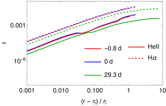
Figure 1: Comparison of the optical-depth radial profiles between the Helium and Hydrogen emission lines obtained by the CLOUDY modeling. The relative radius, $r-r_{l}$, is normalized by the wind inner radius, $r_{l}$. The different colors denote the different time epochs. The solid and dashed lines represent the optical depth of the helium (HeII) and hydrogen (H$\alpha$) emission lines, respectively.

III Disk-wind model

This section briefly describes the disk-wind model (see the appendix A for the details) for fitting the observed continuum spectrum to get values of physical parameters of iPTF16fnl. This model assumes a steady-state, slim disk with an outflow that constitutes the atmosphere [25]. Because the mass accretion rate exceeds the Eddington rate in the slim disk model, the intense radiation pressure induces an outflow [21, 43, 44]. The mass conservation law results in that the sum of the mass accretion rate ($\dot{M}_{\rm a}$) and mass outflow rate ($\dot{M}_{\rm out}$) equals the mass fallback rate of the disrupted stellar debris ($\dot{M}_{\rm fb}$), i.e., $\dot{M}_{\rm a}+\dot{M}_{\rm out}=\dot{M}_{\rm fb}$, where

$$\dot{M}_{\rm fb}=\frac{1}{3}\frac{M_{\star}}{t_{\rm m}}\left(\frac{t_{\rm m}+t}{t_{\rm m}}\right)^{-5/3},$$ (4)

and the period of the most tightly bound debris is given by

$$t_{\rm m}=7.85~{}{\rm days}\,\left(\frac{M_{\bullet}}{10^{6}M_{\odot}}\right)^{1/2}\left(\frac{M_{\star}}{M_{\odot}}\right)^{1/5}\left(\frac{k}{3}\right)^{-3/2}$$ (5)

with the radius of star $R_{\star}=R_{\odot}(M_{\star}/M_{\odot})^{0.8}$ [45]. Here, $k$ is the tidal spin-up factor to take into account the spin-up of a star due to the tidal torque by the black hole [46, 47]. The $k=1$ means the tidal torque is neglected, whereas $k=3$ indicates that the tidal torque spins up the star to its maximum rotational velocity where the centrifugal force exceeds the stellar self-gravity leading to stellar disruption [48]. In our calculation, the time origin $t=0$ corresponds to the fallback time of the most tightly bound debris.

We also assume the mass accretion rate and mass outflow rate are

$$\dot{M}_{\rm out} = f_{0}\,\dot{M}_{\rm fb},$$ (6)

$$\dot{M}_{\rm a} = (1-f_{0})\dot{M}_{\rm fb},$$ (7)

respectively, where $f_{0}$ is given by [5]

$$f_{0}(\eta)={\rm Max}\left[\frac{2}{\pi}{\rm Tan^{-1}}\left\{\frac{1}{4.5}\left(\eta\frac{\dot{M}_{\rm fb}c^{2}}{L_{\rm Edd}}-1\right)\right\},~{}0\right]$$ (8)

and $\eta$ is the radiative efficiency:

$$\eta = \frac{L_{\rm b}}{\dot{M}_{\rm a}c^{2}}$$ (9)

$$= \frac{3R_{\rm S}}{2}\int_{R_{\rm in}}^{R_{\rm out}}\frac{f_{R}}{R^{2}}\left[\frac{1}{2}+\right.$$

$$\left.\sqrt{\frac{1}{4}+\frac{3}{2}f_{R}\left(\frac{R_{\rm S}}{R}\right)^{2}\left(\frac{\dot{M}_{\rm a}}{L_{\rm Edd}/c^{2}}\right)^{2}}~{}\right]^{-1}\,{\text{d}}R,$$

where we use equations (12) and (14) for the derivation, $R_{\rm S}=2GM_{\bullet}/c^{2}$ is the Schwarzschild radius, $f_{R}=1-\sqrt{R_{\rm in}/R}$, $R_{\rm in}$ is the disk inner radius taken to be innermost stable circular orbit of non-spinning black hole, i.e. $R_{\rm in}=3R_{\rm S}$. Note that $\eta$ is not constant for the super-Eddington phase and varies with mass accretion rate.

There are several unknown parameters: black hole mass $M_{\bullet}$, stellar mass $M_{\star}$, wind’s inner radius $r_{l}$, and velocity $v_{\rm w}$. The stellar debris circularizes to form an accretion disk, but the circularization time for the debris is unknown yet very much. Therefore, we also introduce a time parameter $\Delta t$ in the mass fallback rate, which delineates the shift in time $t$ to describe the ambiguity in the starting time of disk accretion after the innermost debris returns to the pericenter. Fitting the disk-wind model to the observed spectral continuum makes it possible to estimate the values of these five unknown parameters directly. The other quantities, such as density, temperatures, and radius of the photosphere, are obtained with these parameters. We will do them in the next section.

III.1 Estimation of five parameters and disk-wind structure

This section estimates the five basic physical quantities and parameters by comparing the observed photometry data and the disk-wind model using the likelihood analysis. Subsequently, those values are used to explore the time evolution of the disk and wind emissions. First, we obtain the photometry data of iPTF16fnl from https://cdsarc.cds.unistra.fr/viz-bin/cat/J/ApJ/844/46#/browse. The host galaxy contaminates the Swift photometry and has very little flux in the Swift UV bands, but the flux dominates in the U, B, and V bands [27]. In our calculation, we neglect Swift U, B, and V bands and instead use the Swift UVW1, UVM2, and UVW2 bands along with the u, g, r, and i bands. To get a continuum with statistically sufficient points, we need to select such observations in different bands that each observed time is nearly equal; at least, the difference in an observed time width of the respective epochs is within a day. In our case, we successfully collected 12 observational epochs, where the difference in the observed time width is $0.7$ days at maximum.

The likelihood at an epoch $i$ is given by $\mathcal{L}_{i}=(\prod_{n=1}^{n=N}\sqrt{2\pi}\sigma_{\rm i,n})^{-1}\exp(-\chi_{i}^{2}/2)$, where $N$ is total number observational points in the epoch $i$, $\sigma_{\rm i,n}$ is the observed uncertainty of the $n$th observation in $i$th epoch, and $\chi_{i}^{2}$ is given by $\chi_{i}^{2}=\sum_{n=1}^{n=N}\left[L^{\rm w}(\nu_{\rm i,n})-L_{\rm i,n}{\rm(obs)}\right]^{2}/\sigma_{\rm i,n}^{2}$. The $L^{\rm w}(\nu_{\rm i,n})$ is the spectral luminosity given by equation (26) for frequency $\nu$ corresponding to $n$th observation and $L_{\rm i,n}{\rm(obs)}$ is the observed luminosity. Since we have 12 epochs of observations, the total likelihood is $\mathcal{L}=\prod_{i=1}^{i=12}\mathcal{L}_{i}$, which results in total $\chi^{2}$ given by

$$\chi^{2}=\sum_{i=1}^{i=12}\chi_{i}^{2}=\sum_{i=1}^{i=12}\sum_{n=1}^{n=N}\frac{\left[L^{\rm w}(\nu_{\rm i,n})-L_{\rm i,n}{\rm(obs)}\right]^{2}}{\sigma_{\rm i,n}^{2}}.$$ (10)

We perform a $\chi^{2}$ minimization simultaneously on all observational data points to obtain the best-fitting parameters: black hole mass, stellar mass, wind inner radius, and wind velocity. With the obtained best-fit parameters, we calculate the Fisher-Information matrix by taking the second derivative of log-likelihood with respect to the free parameters. The inverse of the Fisher matrix represents the covariance matrix, and the square root of diagonal elements of the covariance matrix is the standard error of the parameters.

The resultant five parameters are summarized as follows: $M_{\bullet}=(6.73\pm 0.44)\times 10^{5}M_{\odot}$, $M_{\star}=2.59\pm 0.17M_{\odot}$, $r_{l}=(2.24\pm 0.183)\times 10^{13}~{}{\rm cm}$, $v_{\rm w}=7447.43\pm 183.9~{}{\rm km~{}s^{-1}}$, and $\Delta t=13.25\pm 0.66~{}{\rm days}$. Note that the wind velocity is close to the full-width half maximum (FWHM) of the HeII ($8500\pm 1500~{}{\rm km~{}s^{-1}}$) and H$\alpha$ ($6000\pm 600~{}{\rm km~{}s^{-1}}$) lines at the late time of the observations (see Figure 9 in 27). For the five parameters, we make a test of a relative likelihood: $\bar{\mathcal{L}}=\mathcal{L}/\mathcal{L}_{p}$, where $\mathcal{L}_{p}$ is the likelihood at the obtained parameters. Figure 2 depicts the relative likelihood contours for each parameter. It is noted from the figure that the five parameters lie within 90% of the peak likelihood $\mathcal{L}_{p}$, indicating that those estimated values are statistically well-constrained. Figure 3 makes a comparison between the theoretical spectra with the five parameters and the observed spectra on respective epochs. It is noted from the figure that the theoretical spectra agree well with the observed ones.

According to equations (8) and (9) with equation (7), $f_{0}$ and $\eta$ are a function of time and a complicated dependence on each other. Two panels of Figure 4 depict the solutions for $f_{0}$ and $\eta$, respectively. It is noted from the figure that $f_{0}$ decreases with time, while $\eta$ is almost constant to be a value between $0.01$ and $0.02$ over the observational time.

Figure 5 depicts the wind mass outflow rate and the mass accretion rate of the disk. The Eddington accretion rate,

$$\dot{M}_{\rm Edd}=\frac{1}{\eta}\frac{L_{\rm Edd}}{c^{2}},$$ (11)

normalizes both rates. It is noted from the figure that the mass outflow rate is higher than the mass accretion rate and also decreases with time because of $\dot{M}_{\rm out}=f_{0}\dot{M}_{\rm fb}$. Since $f_{0}$ decreases as the mass fallback rate declines (see equation 4), the time evolution of the mass outflow rate deviates from the $t^{-5/3}$ law of the mass fallback rate. In contrast, the figure shows that the mass accretion rate is almost constant to be $\dot{M}_{\rm a}\approx 2.9\dot{M}_{\rm Edd}$ over time. This is because the increment in $1-f_{0}$ is comparable to the decline in $\dot{M}_{\rm fb}$ for a given mass accretion rate $\dot{M}_{\rm a}=(1-f_{0})\dot{M}_{\rm fb}$, in other words, the effects of those two terms cancel each other out. The constancy of the mass accretion rate is consistent with the steady-state slim disk model.

Figure 6 demonstrates the photospheric radius and temperature of the wind estimated using equations (24) and (25), respectively. It is not trivial to see their time dependency from those equations. However, considering the outflow is expanding with $\dot{M}_{\rm out}\propto t^{-5/3}$ at the constant velocity, the wind density decreases with time, resulting in the photospheric radius is predicted to be smaller with time. Note that the range of the photospheric radius agrees with the blackbody radius ($\sim(0.3-2)\times 10^{14}~{}{\rm cm}$) obtained by Blagorodonova et al. (2017). In contrast, the photosphere temperature increases with time and lies in the range $T_{\rm ph}\in\{1.5,~{}5\}\times 10^{4}~{}{\rm K}$. The increase in the photosphere temperature is slight at late times. The blackbody temperature of the photosphere that Blagorodnova et al. [27] provided is $\sim 2\times 10^{4}~{}{\rm K}$. This is also in good agreement with our photospheric temperature.

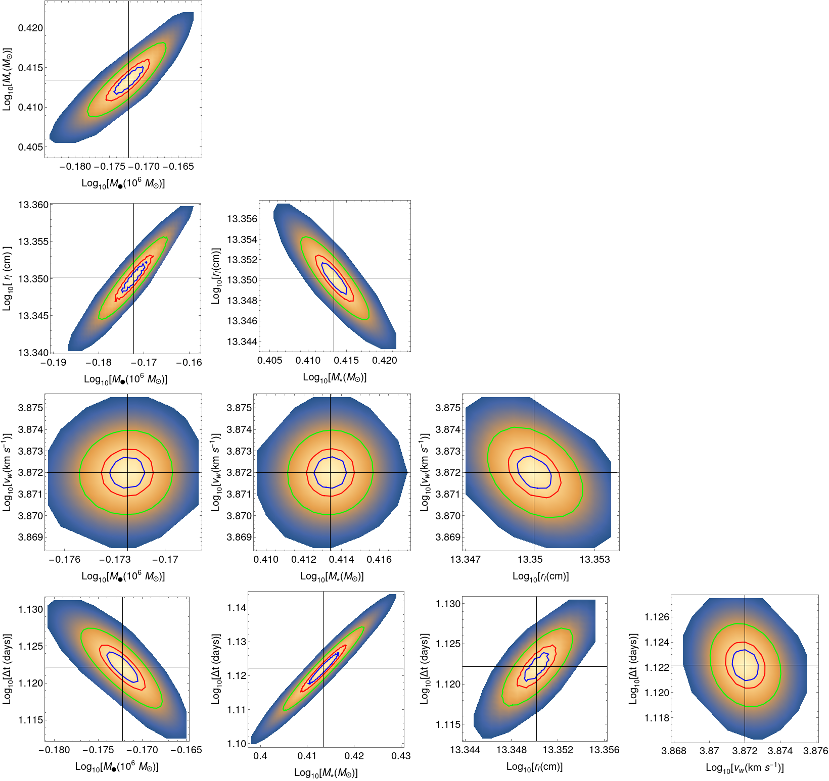
Figure 2: Density contours of the relative likelihood $\bar{\mathcal{L}}=\mathcal{L}/\mathcal{L}_{p}$, where $\mathcal{L}_{p}$ is the likelihood of each parameter, for the five parameters. Here, $\bar{\mathcal{L}}$ is taken to be greater than 0.1. The solid black crossed line delineates $\mathcal{L}_{p}$ of each parameter in each plot. The blue, red, and green circle lines represent the relative likelihood $\bar{\mathcal{L}}=$ $90\%$, $80\%$, and $50\%$, respectively. See section III.1.

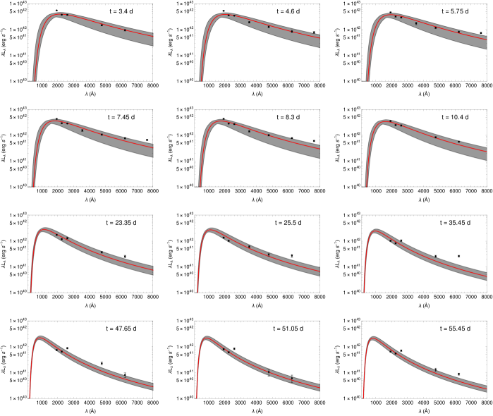
Figure 3: Continuum spectra of iPTF16fnl. The black-filled circles with error bars and the red solid line indicate the observational data and theoretical spectra with the five parameters (see equation 26 for the detail), respectively. The gray-shaded region represents the error range of the theoretical spectrum caused by the five parameters. The corresponding observational epochs are shown at the top right of each panel. See section III.1.

Figure 4: Time evolution of the fraction of mass outflow to fallback rates ($f_{0}$) and the radiative efficiency ($\eta$) connecting between the bolometric luminosity and mass accretion rate. The upper and lower panels display the time evolution of $f_{0}$ and $\eta$, respectively. In both panels, while the black circles indicate $f_{0}$ or $\eta$, which are estimated by equations (8) and (9) with the mean value of the five parameters, the vertical error bars represent the error range caused by the standard deviation of the five parameters.

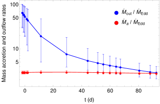
Figure 5: Time dependence of the wind mass outflow rate and disk accretion rate. Both rates are normalized by the Eddington accretion rate. The blue and red lines connected between each filled circle with lines display the mass outflow and accretion rates, respectively. The filled circles delineate the mean value of the five parameters, whereas the error bar per circle corresponds to the standard deviation of the five parameters.

Figure 6: Time evolution of the photospheric radius and the corresponding thermal temperature. Both $r_{\rm ph}$ and $T_{\rm ph}$ are estimated by equation (24) and (25). Panel (a) denotes the time dependence of $r_{\rm ph}$, whereas panel (b) depicts that of $T_{\rm ph}$. In panel (a), the black dashed line represents the wind’s inner radius $r_{l}$. In both panels, the black circles indicate the value estimated using the mean value of the five parameters. The vertical lines represent the error range caused by the standard deviation of the five parameters.

Figure 7: Light curve of the luminosity at the trapping radius (see equation 22). The black-filled circles indicate the luminosity estimated using the mean value of the five parameters. The vertical line per circle represents the error bar corresponding to the standard deviation of the five parameters.

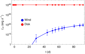
Figure 8: Light curves of X-ray emissions from the disk and wind. The wind X-ray luminosity is calculated at the photospheric radius (see equation 28), while the disk X-ray luminosity is estimated by equation (15). The red- and blue-filled circles indicate the disk and wind X-ray luminosities, respectively, calculated using the five parameters’ mean values. The vertical line per circle represents the error bar corresponding to the standard deviation of the five parameters. Note that the error bars of the disk X-ray luminosity are too small to see in the plot; instead, see the error range in Table 4.

Figure 7 shows the light variation of the wind luminosity given by equation (22) in the diffusion regime of the wind. It is noted that the wind luminosity decreases with time. The peak luminosity is $\sim 1.96\times 10^{43}~{}{\rm erg~{}s^{-1}}$, which agrees with peak bolometric luminosity ($\sim 10^{43}~{}{\rm erg~{}s^{-1}}$) estimated by Blagorodonova et al. (2017) based on a single temperature blackbody model.

Table 4 shows the disk bolometric and X-ray luminosities, which are estimated by equations (14) and (15), respectively. The disk bolometric luminosity, $L_{\rm b}\sim 9.08\times 10^{44}~{}{\rm erg~{}s^{-1}}$, is one order of magnitude higher than the Eddington luminosity, $L_{\rm Edd}=(9.95\pm 0.64)\times 10^{43}~{}{\rm erg~{}s^{-1}}$ with $M_{\bullet}=(6.73\pm 0.44)\times 10^{5}\,M_{\odot}$. This suggests most of the photons emitted from the disk are scattered and absorbed in the media of the outflowing wind so that the detectable photons are emitted at the photosphere of the wind. This results in that the disk bolometric luminosity is reduced to $\lesssim 10^{43}~{}{\rm erg~{}s^{-1}}$ by about three orders of magnitude and observed in the OUV wave bands. In contrast, the X-ray photons are radiated from the sufficiently inner part of the disk. In fact, using equation (12), the peak value of the effective disk temperature is $\sim 4.7\times 10^{5}~{}{\rm K}$, which is about one order of magnitude higher than the photosphere temperature in the wind. As seen in Table 4, the disk X-ray luminosity is estimated to be $L_{\rm X}\sim 10^{40}~{}{\rm erg~{}s^{-1}}$. Figure 8 compares the X-ray light curves of disk and wind emissions, where the wind X-ray emission originates from the photosphere of the wind. It is clear from the figure that the disk X-ray luminosity is much higher than the wind X-ray luminosity, which is calculated by equation (28). As it turns out, the disk X-ray luminosity is low enough to be consistent with the observed X-ray luminosity, $L_{\rm X}\sim 2.4^{+1.9}_{-1.1}\times 10^{39}~{}{\rm erg~{}s^{-1}}$, that Blagorodonova et al. (2017) estimated by stacking all the XRT data over the observation period together (58 ks of total exposure time).

Finally, let us compare the wind densities between CLOUDY and disk-wind models. As seen in Tables 1 and 5, the inner radius estimated from CLOUDY modeling is larger than $r_{\rm l}$, which is calculated from the disk-wind model. Both models assume the mass density to be $\rho\propto r^{-2}$. We compare the wind density estimated from disk-wind and CLOUDY models at the inner radius obtained by CLOUDY. From equation 2, the number density depends on $x$, which is the number density ratio of He over H. Table 5 displays the wind number densities estimated based on the disk-wind model for $x=0.1$ and $x=0.15$, respectively. We note that they correspond to the number densities from the CLOUDY modeling within the error limits.

Table 4: The disk bolometric luminosity and spectral luminosity of the X-ray bands (0.3-10 keV) at ten observational times. The super and subscripts indicate the upper and lower limits of the error range, which corresponds to the standard deviation of the five parameters. The first, second, and third columns represent the observational time, disk bolometric luminosity ($L_{\rm b}$), and spectral X-ray luminosity ($L_{\rm X}$), respectively.

$t~{}{\rm(days)}$	$L_{\rm b}~{}{\rm(10^{44}~{}erg~{}s^{-1})}$	$L_{\rm X}~{}{\rm(10^{40}~{}erg~{}s^{-1})}$
-1.9	$9.081^{+0.24}_{-0.19}$	$1.857^{+0.63}_{-0.63}$
-0.8	$9.093^{+0.23}_{-0.19}$	$1.86^{+0.63}_{-0.63}$
0.0	$9.102^{+0.23}_{-0.20}$	$1.861^{+0.63}_{-0.63}$
1.4	$9.119^{+0.24}_{-0.20}$	$1.863^{+0.64}_{-0.63}$
11.3	$9.246^{+0.21}_{-0.22}$	$1.883^{+0.65}_{-0.66}$
29.3	$9.252^{+0.20}_{-0.19}$	$1.883^{+0.61}_{-0.63}$
44.2	$9.131^{+0.21}_{-0.19}$	$1.865^{+0.63}_{-0.65}$
51.3	$9.065^{+0.21}_{-0.19}$	$1.855^{+0.63}_{-0.65}$
55.2	$4.027^{+0.21}_{-0.19}$	$1.849^{+0.64}_{-0.66}$
88.2	$2.765^{+0.20}_{-0.18}$	$1.795^{+0.67}_{-0.69}$

Table 5: Comparison of the wind number density estimated at $r_{\rm l}=2.51\times 10^{14}~{}{\rm cm}$ between disk-wind model and CLOUDY modeling. The first, second, and third columns represent the observational time, CLOUDY number density, and disk-wind model number density, respectively. For the number density of the disk-wind model, two values of $x$ are adopted.

	CLOUDY	Disk-wind
$t~{}{\rm(days)}$	$\log_{\rm 10}(n_{l}~{}{\rm(cm^{-3})})$	$\log_{\rm 10}(n_{l}~{}{\rm(cm^{-3})})$
		($x=0.1$)	($x=0.15$)
-0.8	10.40	11.55${}^{+1.13}_{-1.11}$	11.49${}^{+1.06}_{-1.05}$
0.0	10.45	11.52${}^{+1.18}_{-1.17}$	11.46${}^{+1.04}_{-1.05}$
29.3	10.20	10.77${}^{+1.2}_{-1.3}$	10.71${}^{+1.2}_{-1.4}$

IV Discussion

iPTF16fnl is an optically discovered low luminosity TDE, and the emission dominates in the UV/optical bands without observationally significant X-ray emission. The host of iPTF16fnl is a post-starburst galaxy with a host velocity dispersion of $89\pm 1~{}{\rm km~{}s^{-1}}$, which were estimated from the CaII $\lambda\lambda$8544,8664 absorption lines. While the black hole mass inferred from the $M_{\bullet}-\sigma$ relation [49] is $(2.138\pm 1.87)\times 10^{6}M_{\odot}$ [27], our model provides the black hole mass to be $M_{\bullet}=(6.73\pm 0.44)\times 10^{5}M_{\odot}$, which agrees with the previous estimate within its error limit. The age of the host galaxy is $650\pm 300~{}{\rm Myr}$ with the metallicity of $Z=0.18$, which nearly equals the solar metallicity $Z_{\odot}=0.2$ [27], suggesting that the host galaxy should have more young main-sequence stars. The elemental abundances in the atmosphere that our CLOUDY modeling provides support this speculation. In that way, our method is useful in probing the nature of the disrupted star.

Our CLOUDY and disk-wind models have obtained the stellar mass of $M_{\star}=2.59\pm 0.17M_{\odot}$. In contrast, the MosFIT model applied to iPTF16fnl provides a stellar mass $M_{\star}=0.101^{+0.008}_{-0.004}M_{\odot}$ [50]. Their evaluated mass is significantly smaller than ours, mainly because the MosFIT model considers no detailed geometry and radiative processes of the wind. Moreover, the MosFIT model assumes constant radiative efficiency and that the photospheric radius and temperature follow the power law of the mass fallback rate, which is the function of the stellar and black hole masses. On the other hand, the CLOUDY modeling demonstrates that the wind is clumpy with a filling factor of 0.8, for the $f=1$ assumption results in more discrepancy in the He II $\lambda$ 4686 line. In addition, from our disk-wind model, the photospheric radius and temperature depend on the wind’s inner radius, mass fallback rate, and radiative efficiency, which is not constant (see equations 9, 24, and 25). The significant deviation of the stellar mass between ours and the MosFit model [50] demonstrates the importance of considering the detailed wind geometry and radiative processes for stellar mass estimation.

Kochanek [51] used Modules for Experiments in Stellar Astrophysics (MESA) model to study the time evolution of the element abundances within the star, assuming the star has the solar metallicity at the initial time. Since the Sun’s helium and other elements fractions are significantly smaller than hydrogen, the helium-to-hydrogen number ratio is set to be $\sim 0.09$ at the initial time. For a stellar mass of $2\,M_{\odot}$, he showed that the helium abundance increases by $\sim 1.12\times{\rm initial~{}helium~{}abundance}$ after a stellar evolution time of 1 Gyr. The nitrogen abundance increases by $\sim 1.6\times{\rm initial~{}nitrogen~{}abundance}$, whereas the carbon abundance decreases. The increment in helium abundance is small. Since the host galaxy has an age of 650 $\pm$ 300 Myr with a metallicity of 0.18, we can expect a low increment in the helium abundance within the star if its metallicity at the initial time is close to the solar metallicity. This complements our CLOUDY estimation of a small helium-to-hydrogen number ratio, indicating that the disrupted star has a low helium abundance.

In our disk-wind model, the radiative efficiency $\eta$ varies with time due to the time-dependent mass fallback rate, as shown in equation (9). The proportionality coefficient $f_{0}$ goes to zero if $\dot{M}_{\rm fb}\leq\dot{M}_{\rm Edd}$, indicating no outflow so that the radiative efficiency is constant in time because $f_{0}$ is independent of the mass fallback rate. Moreover, our calculation demonstrates that $0.01\lesssim\eta\lesssim 0.02$, indicating that the disk is radiatively inefficient. Figure 5 depicts that the mass outflow rate decreases with time rapidly whereas the mass accretion rate has little time variation. Considering that the ratio of mass accretion to outflow rates is given by $\dot{M}_{\rm out}/\dot{M}_{\rm a}=f_{0}/(1-f_{0})$, we obtain the condition, by using equation (8), that $\dot{M}_{\rm fb}<5.5~{}\dot{M}_{\rm Edd}$ when $\dot{M}_{\rm out}$ is lower than $\dot{M}_{\rm a}$. Combining equations (4) and (11) find $t\sim 96~{}{\rm days}$ for $\dot{M}_{\rm fb}=5.5~{}\dot{M}_{\rm Edd}$. The significantly low mass outflow rate at such late times makes the photosphere radius lower, resulting in lower thermal luminosity.

We have assumed that there is no dynamical interaction with ambient matter around the SMBH in our disk-wind model. More realistically, however, the interaction between the ambient mass and the outflow can occur and consequently create a shocked region from which non-thermal radiations, such as radio emission, are emitted. In fact, several radio-emitting TDEs, even without a relativistic jet, have been observed so far [52]. To explore some mechanism for radio emission from radio-emitting, non-jetted TDE AT2019dsg [53], the theoretical work with a thin shell approximation has recently been done by Hayasaki and Yamazaki [54]. Constructing a unified model to reproduce observational thermal and non-thermal emissions from TDEs is also our future task.

The observations of iPTF16fnl around the peak luminosity demonstrate the FWHM of the helium line to be $\sim 14000\pm 3000\,{\rm km~{}s^{-1}}$, whereas the hydrogen line has an FWHM of $\sim 10000\pm 500~{}{\rm km~{}s^{-1}}$. Moreover, at late times, the FWHM reduces to $\sim 8500\pm 1500\,{\rm km~{}s^{-1}}$ for helium HeII line and $6000\pm 600~{}{\rm km~{}s^{-1}}$ for hydrogen H$\alpha$ line [27]. On the other hand, CLOUDY modeling provides that the FWHM on 29.3 days is $\sim 7500$ km s^-1 and $\sim 4200$ km s^-1 for the HeII and H$\alpha$ lines, respectively. We find that the FWHM of H$\alpha$ is clearly underestimated at late times although the HeII line agrees with the observations. However, note that the CLOUDY-modeled line luminosities agree with the observations, as described in Section II.2. Those findings suggest that the discrepancy of the FWHM of H$\alpha$ between the observation and CLOUDY modeling originates from the assumption that the motion of wind gas is steady. Realistically, the gas in the wind can accelerate due to the radially declining black hole gravity and the radiation force from photons. Therefore, we need to relax our steady-state assumption and apply time-dependent CLOUDY modeling to explore the FHWM discrepancy problem.

The center of spectral lines appears constant within the scatter for the first 90 days. The HeII line seems marginally blue-shifted with a velocity of $-700\pm 700~{}{\rm km~{}s^{-1}}$. However, this shift in line velocity lies within the FWHM. The H$\alpha$ line is consistent with the reference wavelength. This suggests the spectrum of iPTF16fnl is symmetric about the central wavelength of the spectral line. Our disk-wind model assumes a spherical distribution extending up to a large distance such that the wind outer radius $r_{\rm w,o}\gg r_{l}$ and the wind velocity is constant at all the radii. This simple assumption is appropriate for TDEs showing symmetric line profiles. In future work, we will consider a time-varying wind velocity and/or a non-spherical wind geometry to explain asymmetric spectral line profiles.

V Summary

iPTF16fnl is a low redshift and optically low luminosity TDE with no significant X-ray observations, indicating the presence of an atmosphere that obscures the disk radiation and emits in UV/optical bands. The observed line signatures demonstrate that the Helium spectral lines dominate over the hydrogen lines at early times, and the luminosity ratio of helium to hydrogen lines decreases with time. Our paper aims to elucidate the physical properties of the atmosphere necessary for the observed spectrum continuum and line luminosity. We have estimated five unknown physical parameters by fitting the steady-state slim disk with a spherical wind model (i.e., disk-wind model) to the spectrum continuum at ten observed time epochs. Moreover, we have studied why the helium line dominates over the hydrogen line by comparing the predicted lines by CLOUDY modeling with the observational spectral lines at three observed time epochs. Our key findings are summarized as follows:

1. We find the black hole mass is $M_{\bullet}=(6.73\pm 0.44)\times 10^{5}M_{\odot}$, the stellar mass is $M_{\star}=(2.59\pm 0.17)M_{\odot}$, the wind inner radius is $r_{l}=(2.24\pm 0.183)\times 10^{13}~{}{\rm cm}$, the wind velocity is $v_{\rm w}=7447.43\pm 183.9~{}{\rm km~{}s^{-1}}$, and the disk formation time is $\Delta t=13.25\pm 0.66~{}{\rm days}$. Note that the time origin of our model is the time when debris with the most tightly bound orbit returns to the pericenter.

2. In our disk-wind model, the radiative efficiency depends on the black hole mass and the mass accretion rate, indicating that the bolometric luminosity is not simply proportional to the mass accretion rate (see equation 9). We find the radiative efficiency to be $0.01\lesssim\eta\lesssim 0.02$ over the observational time, resulting in the disk being radiatively inefficient. The resultant X-ray luminosity is estimated to be $\sim 10^{40}\,{\rm erg\,s^{-1}}$ over the observational time, which is consistent with the observed X-ray luminosity.

3. The mass outflow rate dominates the mass accretion rate at early times, but the mass outflow rate declines rapidly compared to the mass accretion rate. The significant decay of the mass outflow rate reduces the wind density so that the photosphere radius decreases with time. We confirm the photospheric radius agrees with the blackbody radius estimated by Blagorodonova (2017).

4. The photosphere temperature increases with time from $\sim 15000~{}{\rm K}$ to $\sim 50000~{}{\rm K}$. The peak bolometric luminosity at the photosphere ($\sim 1.96\times 10^{43}~{}{\rm erg~{}s^{-1}}$) is in good agreement with the observed OUV luminosity ($\sim 10^{43}~{}{\rm erg~{}s^{-1}}$). In contrast, the disk luminosity in soft-X-ray wavebands is low enough to support the dominance of optical/UV observations.

5. The CLOUDY modeling shows that the medium is generally inhomogeneous and clumpy. We estimate the filling factor to be 0.8, indicating that the gas occupies $80\%$ of the atmosphere as clumps while the remaining $20\%$ is a vacuum.

6. The CLOUDY modeling finds that the helium-to-hydrogen number ratio, $x$, lies between 0.1 and 0.15. The low metallicity of the host galaxy supports this range of $x$. The low value of $x$, which is comparable to $x\sim 0.1$ for the sun, suggests the disrupted star originally is a main-sequence star. The CLOUDY modeling also demonstrates that the optical depth for the hydrogen emission line is two orders of magnitude higher than the helium emission line. Considering the helium abundance is $10\%$ to $15\%$ of the hydrogen, we conclude that the dominance of the helium emission line over the hydrogen emission line is due to the optical depth effect.

VI acknowledgments

GS acknowledges WOS-A grant from the Department of Science and Technology (SR/WOS-A/PM-2/2021). Two authors have been supported by the Basic Science Research Program through the National Research Foundation of Korea (NRF) funded by the Ministry of Education (2016R1A5A1013277 to K.H. and 2020R1A2C1007219 to K.H. and M.T.)

VII Data Availability

Simulations in this paper made use of freely downloadable code CLOUDY (https://www.nublado.org, C17.02). The photometry data for the continuum is available at https://cdsarc.cds.unistra.fr/viz-bin/cat/J/ApJ/844/46#/browse. The model-generated data are available on request.

Appendix A Disk wind model details

In this section, we present the disk-wind model in detail. We consider a steady-state, radiation-pressure dominant, slim dis model with a super-Eddington accretion rate. The strong radiation pressure induces an outflow [21, 43, 44]. In the slim disk model, the advection energy cooling is essential for the thermal stability of the disk with radiation pressure, reducing the amount of viscous heating flux radiated and the scale height of a slim disk is $H\sim R$ [55, 21], where $R$ is the disk radius at the disk mid-plane. In a steady-state super-Eddington disk with an outflow, the mass conservation law gives equations (7) and (7). These equations represent $f_{0}$ as a key parameter to decide the evolution of both rates. Dotan and Shaviv [56] numerically simulated $f_{0}$ at the outer radius for a steady disk and showed that $f_{0}$ is approximated into empirical relation shown as equation (8). Although Strubbe and Quataert [21] assumed $f_{0}$ to be a constant, our model demonstrates that $f_{0}$ is not a constant because $\eta$ is also not constant, as seen in equations (8) and (9). The radiative flux from a super-Eddington disk with radiation pressure is given by [21] as

$$\sigma T_{\rm eff}^{4}=\frac{3GM_{\bullet}\dot{M}_{\rm a}f_{R}}{8\pi R^{3}}\times\\ \left[\frac{1}{2}+\sqrt{\frac{1}{4}+\frac{3}{2}f_{R}\left(\frac{\dot{M}_{\rm a}}{L_{\rm Edd}/c^{2}}\right)^{2}\left(\frac{R}{R_{\rm S}}\right)^{-2}}\right]^{-1},$$ (12)

where $\sigma$ is the Stefan-Boltzmann constant. $R_{\rm S}=2GM_{\bullet}/c^{2}$ is the Schwarzschild radius, $f_{R}=1-\sqrt{R_{\rm in}/R}$, and $R_{\rm in}$ is the disk inner radius taken to be innermost stable circular orbit of non-spinning black hole, i.e. $R_{\rm in}=3R_{\rm S}$. A similar formula as the above equation for the radiative to advection cooling rate for a general relativistic slim disk model with radiation pressure was constructed by Mageshwaran and Hayasaki [57]. The observed flux from the disk is given by [55]

$$F=\frac{\cos\theta_{\rm los}}{D_{\rm L}^{2}}\int_{\nu_{\rm l}}^{\nu_{\rm h}}\int_{R_{\rm in}}^{R_{\rm out}}B(T_{\rm eff},~{}\nu)2\pi R\,{\text{d}}R\,{\text{d}}\nu,$$ (13)

where $R_{\rm out}$ is the disk outer radius, $B(T_{\rm eff},~{}\nu)$ is the blackbody Planck function, $\nu$ is the frequency, $\nu_{\rm l}$ and $\nu_{\rm h}$ are the lower and upper frequency respectively, $D_{\rm L}$ is the luminosity distance of the source to the observer and $\theta_{\rm los}$ is the is the angle between observer line-of-sight and disk normal vector. Adopting $\theta_{\rm los}=0^{\circ}$ for equation (13), we obtain the observed luminosity as

$$L = 4\pi D_{\rm L}^{2}F$$

$$= 8\pi^{2}\int_{\nu_{\rm l}}^{\nu_{\rm h}}\int_{R_{\rm in}}^{R_{\rm out}}B(T_{\rm eff},~{}\nu)R\,{\text{d}}R\,{\text{d}}\nu.$$

The bolometric luminosity is obtained by applying $\nu_{\rm l}=0$ and $\nu_{\rm h}=\infty$ to the above equation as

$$L_{\rm b}=8\pi\int_{R_{\rm in}}^{R_{\rm out}}\sigma T_{\rm eff}^{4}R\,{\text{d}}R.$$ (14)

The X-ray luminosity with the energy range 0.3-10 keV is estimated to be

$$L_{\rm X}=8\pi^{2}\cos\theta_{\rm los}\int_{\nu_{\rm l,X}}^{\nu_{\rm h,X}}\int_{R_{\rm in}}^{R_{\rm out}}B(T_{\rm eff},~{}\nu)R\,{\text{d}}R\,{\text{d}}\nu,$$ (15)

where the corresponding frequency range is from $\nu_{\rm l,X}=7.2\times 10^{16}\,{\rm Hz}$ to $\nu_{\rm h,X}=2.4\times 10^{18}$ Hz.

We assume that the wind is blowing spherically from the disk with the constant velocity $v_{\rm w}$ and mass outflow rate $\dot{M}_{\rm out}$. The radial density profile of the wind is then given by

$$\rho(r)=\frac{\dot{M}_{\rm out}}{4\pi r^{2}v_{\rm w}},$$ (16)

where $\dot{M}_{\rm out}=f_{0}\dot{M}_{\rm fb}$ (see equation 7). We also assume that the wind is launched at the inner radius of the wind, $r_{\rm l}$ and the outer radius of the wind $r_{\rm w,o}$ is much larger than the inner radius, i.e., $r_{\rm w,o}\gg r_{l}$. The optical depth $\tau$ with an opacity dominated by electron scattering is given by

$$\tau_{\rm es}(r)=\int_{r}^{r_{\rm w,o}}\kappa_{\rm es}\rho(r)\,{\text{d}}r\approx\kappa_{\rm es}\frac{\dot{M}_{\rm out}}{4\pi v_{\rm w}r}.$$ (17)

Considering the kinetic energy density of the wind, $(1/2)\rho(r)v_{\rm w}^{2}$, is in equilibrium with the internal energy density dominated by the radiation, $aT_{l}^{4}$, [21], we obtain the temperature $T_{l}$ at the inner radius of the wind as

$$T_{l}=\left(\frac{\dot{M}_{\rm out}v_{\rm w}}{8\pi r_{l}^{2}a}\right)^{1/4},$$ (18)

where $a$ is the radiation constant.

If the photon diffusion time is longer than the dynamical time of the wind, the photons are trapped and coupled with the matter. By equating the photon diffusion timescale, $t_{\rm diff}=\tau_{\rm es}(r)r/c$, with the dynamical time of the wind, $t_{\rm dyn}=(r-r_{l})/v_{\rm w}$, we obtain the photon trapping radius as

$$r_{\rm tr}=r_{l}+\frac{\kappa_{\rm es}\dot{M}_{\rm out}}{4\pi c}.$$ (19)

For $r<r_{\rm tr}$, the photons are advected without escaping outside so that the temperature evolves adiabatically. Since the adiabatic temperature is given by $T\propto\rho(r)^{1/3}\propto r^{-2/3}$, the temperature at the trapping radius is given by

$$T_{\rm tr}=T_{l}\left(\frac{r_{\rm tr}}{r_{l}}\right)^{-2/3}.$$ (20)

For $r>r_{\rm tr}$, the photons diffuse in the wind at a power:

$$L_{\rm w}=-\frac{4\pi r^{2}ac}{3\kappa_{\rm es}\rho(r)}\frac{\partial T^{4}}{\partial r}.$$ (21)

Considering the luminosity is nearly constant in the diffusive regime [24], the temperature evolves as $T\propto r^{-3/4}$. Substituting equations (16) to (20) into equation (21) with $T\propto{r^{-3/4}}$ gives the luminosity at the trapping radius as

$$L_{\rm ph}=\frac{2\pi c}{\kappa_{\rm es}}v_{\rm w}^{2}r_{l}\left(\frac{r_{\rm tr}}{r_{l}}\right)^{1/3}.$$ (22)

In the diffusive region, apart from electron scattering, the absorption of photons by electrons can also be a source of opacity. Thus, total opacity is given by $\kappa_{\rm eff}\approx\sqrt{3\kappa_{\rm es}\kappa_{a}}$, where the absorption opacity is taken to be the Kramers opacity, $\kappa_{a}=\kappa_{0}\rho T^{-7/2}~{}{\rm cm^{2}~{}g^{-1}}$. Such a color radius that the optical depth is unity, which is obtained by imposing $\tau_{\rm es}(r=r_{\rm cl})=1$ on equation (17), is given by [24].

$$r_{\rm cl}=\left(\frac{16}{11}\right)^{16/11}\left(3\kappa_{\rm es}\kappa_{0}\right)^{8/11}\left(\frac{\dot{M}_{\rm out}}{4\pi v_{\rm w}}\right)^{24/11}r_{\rm tr}^{-21/11}T_{\rm tr}^{-28/11}.$$ (23)

The photospheric radius is given by

$$r_{\rm ph}={\rm Max[}r_{\rm tr},~{}r_{\rm cl}{\rm]}\approx r_{\rm tr}$$ (24)

for appropriate parameters. So, we confirm that equation (22) corresponds to the luminosity at the photosphere. The photospheric temperature is then given by

$$T_{\rm ph}=\left(\frac{L_{\rm ph}}{4\pi r_{\rm ph}^{2}\sigma}\right)^{1/4},$$ (25)

where where we use equation (22) for the derivation. Assuming a blackbody emission from the photosphere, we obtain the effective luminosity at a given frequency as [58]

$$L^{\rm w}(\nu)=\nu L_{\nu,\rm ph}=\nu~{}4\pi r_{\rm ph}^{2}\frac{2h\nu^{3}}{c^{2}}\left[\exp\Big{(}\frac{h\nu}{k_{B}T_{\rm ph}}\Big{)}-1\right]^{-1}$$ (26)

with the spectral luminosity at the photosphere:

$$L_{\nu,\rm ph}\equiv 4\pi r_{\rm ph}^{2}\frac{2h\nu^{3}}{c^{2}}\left[\exp\Big{(}\frac{h\nu}{k_{B}T_{\rm ph}}\Big{)}-1\right]^{-1}.$$ (27)

The X-ray luminosity at the photosphere in the range of $0.3-10$ keV is calculated by

$$L_{X,\rm ph} = \int_{\nu_{\rm l,X}}^{\nu_{\rm h,X}}L_{\nu,\rm ph}\,d\nu$$

$$= \frac{8\pi hr_{\rm ph}^{2}}{c^{2}}\int_{\nu_{\rm l,X}}^{\nu_{\rm h,X}}\nu^{3}\left[\exp\Big{(}\frac{h\nu}{k_{B}T_{\rm ph}}\Big{)}-1\right]^{-1}\,d\nu,$$

(28)

where the values of $\nu_{\rm l,X}$ and $\nu_{\rm h,X}$ are seen below equation (15).

References

- Frank and Rees [1976] J. Frank and M. J. Rees, Effects of massive central black holes on dense stellar systems, Mon. Not. Roy. Astron. Soc. 176, 633 (1976).
- Rees [1988] M. J. Rees, Tidal disruption of stars by black holes of 10 to the 6th-10 to the 8th solar masses in nearby galaxies, Nature (London) 333, 523 (1988).
- Guillochon and Ramirez-Ruiz [2013] J. Guillochon and E. Ramirez-Ruiz, Hydrodynamical Simulations to Determine the Feeding Rate of Black Holes by the Tidal Disruption of Stars: The Importance of the Impact Parameter and Stellar Structure, Astrophys. J. 767, 25 (2013), arXiv:1206.2350 [astro-ph.HE] .
- Lodato et al. [2009] G. Lodato, A. R. King, and J. E. Pringle, Stellar disruption by a supermassive black hole: is the light curve really proportional to t-5/3?, Mon. Not. Roy. Astron. Soc. 392, 332 (2009), arXiv:0810.1288 .
- Mageshwaran and Mangalam [2015] T. Mageshwaran and A. Mangalam, Stellar and Gas Dynamical Model for Tidal Disruption Events in a Quiescent Galaxy, Astrophys. J. 814, 141 (2015), arXiv:1510.07828 .
- Golightly et al. [2019] E. C. A. Golightly, E. R. Coughlin, and C. J. Nixon, Tidal Disruption Events: The Role of Stellar Spin, Astrophys. J. 872, 163 (2019), arXiv:1901.03717 [astro-ph.HE] .
- Hayasaki et al. [2018] K. Hayasaki, S. Zhong, S. Li, P. Berczik, and R. Spurzem, Classification of Tidal Disruption Events Based on Stellar Orbital Properties, Astrophys. J. 855, 129 (2018), arXiv:1802.06798 [astro-ph.HE] .
- Park and Hayasaki [2020] G. Park and K. Hayasaki, Tidal Disruption Flares from Stars on Marginally Bound and Unbound Orbits, Astrophys. J. 900, 3 (2020), arXiv:2001.04548 [astro-ph.HE] .
- Zhong et al. [2023] S. Zhong, K. Hayasaki, S. Li, P. Berczik, and R. Spurzem, Exploring the Origin of Stars on Bound and Unbound Orbits Causing Tidal Disruption Events, Astrophys. J. 959, 19 (2023), arXiv:2011.09400 [astro-ph.HE] .
- Cufari et al. [2022] M. Cufari, E. R. Coughlin, and C. J. Nixon, The Eccentric Nature of Eccentric Tidal Disruption Events, Astrophys. J. 924, 34 (2022), arXiv:2110.11374 [astro-ph.HE] .
- Hayasaki et al. [2013] K. Hayasaki, N. Stone, and A. Loeb, Finite, intense accretion bursts from tidal disruption of stars on bound orbits, Mon. Not. Roy. Astron. Soc. 434, 909 (2013), arXiv:1210.1333 [astro-ph.HE] .
- Hayasaki et al. [2016] K. Hayasaki, N. Stone, and A. Loeb, Circularization of tidally disrupted stars around spinning supermassive black holes, Mon. Not. Roy. Astron. Soc. 461, 3760 (2016), arXiv:1501.05207 [astro-ph.HE] .
- Bonnerot et al. [2016] C. Bonnerot, E. M. Rossi, G. Lodato, and D. J. Price, Disc formation from tidal disruptions of stars on eccentric orbits by Schwarzschild black holes, Mon. Not. Roy. Astron. Soc. 455, 2253 (2016), arXiv:1501.04635 [astro-ph.HE] .
- Bonnerot and Lu [2020] C. Bonnerot and W. Lu, Simulating disc formation in tidal disruption events, Monthly Notices of the Royal Astronomical Society 495, 1374 (2020), aDS Bibcode: 2020MNRAS.495.1374B.
- Lu and Bonnerot [2020] W. Lu and C. Bonnerot, Self-intersection of the fallback stream in tidal disruption events, Monthly Notices of the Royal Astronomical Society 492, 686 (2020), aDS Bibcode: 2020MNRAS.492..686L.
- Holoien et al. [2016a] T. W.-S. Holoien, C. S. Kochanek, J. L. Prieto, K. Z. Stanek, S. Dong, B. J. Shappee, D. Grupe, J. S. Brown, U. Basu, J. F. Beacom, D. Bersier, J. Brimacombe, A. B. Danilet, E. Falco, Z. Guo, J. Jose, G. J. Herczeg, F. Long, G. Pojmanski, G. V. Simonian, D. M. Szczygieł, T. A. Thompson, J. R. Thorstensen, R. M. Wagner, and P. R. Woźniak, Six months of multiwavelength follow-up of the tidal disruption candidate ASASSN-14li and implied TDE rates from ASAS-SN, Mon. Not. Roy. Astron. Soc. 455, 2918 (2016a), arXiv:1507.01598 [astro-ph.HE] .
- Saxton et al. [2014] R. D. Saxton, A. M. Read, S. Komossa, P. Rodriguez-Pascual, G. Miniutti, P. Dobbie, P. Esquej, M. Colless, and K. W. Bannister, An X-ray and UV flare from the galaxy XMMSL1 J061927.1-655311, Astron. & Astrophys. 572, A1 (2014), arXiv:1410.1500 [astro-ph.HE] .
- Maksym et al. [2013] W. P. Maksym, M. P. Ulmer, M. C. Eracleous, L. Guennou, and L. C. Ho, A tidal flare candidate in Abell 1795, Mon. Not. Roy. Astron. Soc. 435, 1904 (2013), arXiv:1307.6556 [astro-ph.HE] .
- Esquej et al. [2007] P. Esquej, R. D. Saxton, M. J. Freyberg, A. M. Read, B. Altieri, M. Sanchez-Portal, and G. Hasinger, Candidate tidal disruption events from the XMM-Newton slew survey, Astron. & Astrophys. 462, L49 (2007), astro-ph/0612340 .
- Dai et al. [2018] L. Dai, J. C. McKinney, N. Roth, E. Ramirez-Ruiz, and M. C. Miller, A Unified Model for Tidal Disruption Events, Astrophys. J. Lett. 859, L20 (2018), arXiv:1803.03265 [astro-ph.HE] .
- Strubbe and Quataert [2009] L. E. Strubbe and E. Quataert, Optical flares from the tidal disruption of stars by massive black holes, Mon. Not. Roy. Astron. Soc. 400, 2070 (2009), arXiv:0905.3735 [astro-ph.CO] .
- Piro and Lu [2020] A. L. Piro and W. Lu, Wind-reprocessed Transients, Astrophys. J. 894, 2 (2020), arXiv:2001.08770 [astro-ph.HE] .
- Roth et al. [2020] N. Roth, E. M. Rossi, J. Krolik, T. Piran, B. Mockler, and D. Kasen, Radiative Emission Mechanisms, Space Sci. Rev. 216, 114 (2020), arXiv:2008.01117 [astro-ph.HE] .
- Uno and Maeda [2020] K. Uno and K. Maeda, A Wind-driven Model: Application to Peculiar Transients AT2018cow and iPTF14hls, Astrophys. J. 897, 156 (2020), arXiv:2003.05795 [astro-ph.HE] .
- Mageshwaran et al. [2023] T. Mageshwaran, G. Shaw, and S. Bhattacharyya, Probing the tidal disruption event iPTF16axa with CLOUDY and disc-wind models, Mon. Not. Roy. Astron. Soc. 518, 5693 (2023), arXiv:2211.14458 [astro-ph.HE] .
- Holoien et al. [2016b] T. W.-S. Holoien, C. S. Kochanek, J. L. Prieto, D. Grupe, P. Chen, D. Godoy-Rivera, K. Z. Stanek, B. J. Shappee, S. Dong, J. S. Brown, U. Basu, J. F. Beacom, D. Bersier, J. Brimacombe, E. K. Carlson, E. Falco, E. Johnston, B. F. Madore, G. Pojmanski, and M. Seibert, ASASSN-15oi: a rapidly evolving, luminous tidal disruption event at 216 Mpc, Mon. Not. Roy. Astron. Soc. 463, 3813 (2016b), arXiv:1602.01088 [astro-ph.HE] .
- Blagorodnova et al. [2017] N. Blagorodnova, S. Gezari, T. Hung, S. R. Kulkarni, S. B. Cenko, D. R. Pasham, L. Yan, I. Arcavi, S. Ben-Ami, B. D. Bue, T. Cantwell, Y. Cao, A. J. Castro-Tirado, R. Fender, C. Fremling, A. Gal-Yam, A. Y. Q. Ho, A. Horesh, G. Hosseinzadeh, M. M. Kasliwal, A. K. H. Kong, R. R. Laher, G. Leloudas, R. Lunnan, F. J. Masci, K. Mooley, J. D. Neill, P. Nugent, M. Powell, A. F. Valeev, P. M. Vreeswijk, R. Walters, and P. Wozniak, iPTF16fnl: A Faint and Fast Tidal Disruption Event in an E+A Galaxy, Astrophys. J. 844, 46 (2017), arXiv:1703.00965 [astro-ph.HE] .
- Hung et al. [2017] T. Hung, S. Gezari, N. Blagorodnova, N. Roth, S. B. Cenko, S. R. Kulkarni, A. Horesh, I. Arcavi, C. McCully, L. Yan, R. Lunnan, C. Fremling, Y. Cao, P. E. Nugent, and P. Wozniak, Revisiting Optical Tidal Disruption Events with iPTF16axa, Astrophys. J. 842, 29 (2017), arXiv:1703.01299 [astro-ph.HE] .
- Roth et al. [2016] N. Roth, D. Kasen, J. Guillochon, and E. Ramirez-Ruiz, The X-Ray through Optical Fluxes and Line Strengths of Tidal Disruption Events, Astrophys. J. 827, 3 (2016), arXiv:1510.08454 [astro-ph.HE] .
- Strubbe and Murray [2015] L. E. Strubbe and N. Murray, Insights into tidal disruption of stars from PS1-10jh, Mon. Not. Roy. Astron. Soc. 454, 2321 (2015), arXiv:1509.04277 [astro-ph.HE] .
- Gezari et al. [2016] S. Gezari, T. Hung, N. Blagorodnova, J. D. Neill, L. Yan, S. Kulkarni, S. B. Cenko, I. Arcavi, G. Hosseinzadeh, A. Horesh, A. Gal-Yam, G. Leloudas, R. Walters, S. Ben-Ami, Y. Cao, A. Miller, F. Masci, and P. Nugent, iPTF16fnl: Likely Tidal Disruption Event at 65 Mpc, The Astronomer’s Telegram 9433, 1 (2016).
- Brown et al. [2018] J. S. Brown, C. S. Kochanek, T. W. S. Holoien, K. Z. Stanek, K. Auchettl, B. J. Shappee, J. L. Prieto, N. Morrell, E. Falco, J. Strader, L. Chomiuk, R. Post, J. Villanueva, S., S. Mathur, S. Dong, P. Chen, and S. Bose, The ultraviolet spectroscopic evolution of the low-luminosity tidal disruption event iPTF16fnl, Mon. Not. Roy. Astron. Soc. 473, 1130 (2018), arXiv:1704.02321 [astro-ph.HE] .
- Ferland et al. [2017] G. J. Ferland, M. Chatzikos, F. Guzmán, M. L. Lykins, P. A. M. van Hoof, R. J. R. Williams, N. P. Abel, N. R. Badnell, F. P. Keenan, R. L. Porter, and P. C. Stancil, The 2017 Release Cloudy, Revista Mexicana de Astronomía y Astrofísica 53, 385 (2017), arXiv:1705.10877 [astro-ph.GA] .
- Ferland et al. [2013] G. J. Ferland, R. L. Porter, P. A. M. van Hoof, R. J. R. Williams, N. P. Abel, M. L. Lykins, G. Shaw, W. J. Henney, and P. C. Stancil, The 2013 Release of Cloudy, Revista Mexicana de Astronomía y Astrofísica 49, 137 (2013), arXiv:1302.4485 [astro-ph.GA] .
- Shaw et al. [2022] G. Shaw, G. J. Ferland, and M. Chatzikos, Recent Updates to the Gas-phase Chemical Reactions and Molecular Lines in CLOUDY: Their Effects on Millimeter and Submillimeter Molecular Line Predictions, Astrophys. J. 934, 53 (2022), arXiv:2206.04606 [astro-ph.GA] .
- Pandey et al. [2022] R. Pandey, R. Das, G. Shaw, and S. Mondal, Photoionization Modeling of the Dusty Nova V1280 Scorpii, Astrophys. J. 925, 187 (2022), arXiv:2111.02380 [astro-ph.SR] .
- Mondal et al. [2019] A. Mondal, R. Das, G. Shaw, and S. Mondal, A photoionization model grid for novae: estimation of physical., Mon. Not. Roy. Astron. Soc. 483, 4884 (2019), arXiv:1811.06727 [astro-ph.SR] .
- Davies et al. [2020] R. Davies, D. Baron, T. Shimizu, H. Netzer, L. Burtscher, P. T. de Zeeuw, R. Genzel, E. K. S. Hicks, M. Koss, M. Y. Lin, D. Lutz, W. Maciejewski, F. Müller-Sánchez, G. Orban de Xivry, C. Ricci, R. Riffel, R. A. Riffel, D. Rosario, M. Schartmann, A. Schnorr-Müller, J. Shangguan, A. Sternberg, E. Sturm, T. Storchi-Bergmann, L. Tacconi, and S. Veilleux, Ionized outflows in local luminous AGN: what are the real densities and outflow rates?, Mon. Not. Roy. Astron. Soc. 498, 4150 (2020), arXiv:2003.06153 [astro-ph.GA] .
- Parkinson et al. [2020] E. J. Parkinson, C. Knigge, K. S. Long, J. H. Matthews, N. Higginbottom, S. A. Sim, and H. A. Hewitt, Accretion disc winds in tidal disruption events: ultraviolet spectral lines as orientation indicators, Mon. Not. Roy. Astron. Soc. 494, 4914 (2020), arXiv:2004.07727 [astro-ph.HE] .
- Ferland [2006] G. J. Ferland, Hazy, A Brief Introduction to Cloudy 06.02 (2006).
- Grevesse et al. [2010] N. Grevesse, M. Asplund, A. J. Sauval, and P. Scott, The chemical composition of the Sun, Astrophys. Space Sci. 328, 179 (2010).
- Grevesse and Sauval [1998] N. Grevesse and A. J. Sauval, Standard Solar Composition, Space Sci. Rev. 85, 161 (1998).
- Cao and Gu [2015] X. Cao and W.-M. Gu, Limits on luminosity and mass accretion rate of a radiation-pressure-dominated accretion disc, Mon. Not. Roy. Astron. Soc. 448, 3514 (2015), arXiv:1502.02892 [astro-ph.HE] .
- Feng et al. [2019] J. Feng, X. Cao, W.-M. Gu, and R.-Y. Ma, A Global Solution to a Slim Accretion Disk with Radiation-driven Outflows, Astrophys. J. 885, 93 (2019), arXiv:1909.07559 [astro-ph.HE] .
- Kippenhahn and Weigert [1994] R. Kippenhahn and A. Weigert, Stellar Structure and Evolution, XVI, 468 pp. 192 figs.. Springer-Verlag Berlin Heidelberg New York. Also Astronomy and Astrophysics Library (Springer-Verlag press, Berlin Heidelberg New York, 1994).
- Alexander and Kumar [2001] T. Alexander and P. Kumar, Tidal Spin-up of Stars in Dense Stellar Cusps around Massive Black Holes, Astrophys. J. 549, 948 (2001), astro-ph/0004240 .
- Mageshwaran and Bhattacharyya [2020] T. Mageshwaran and S. Bhattacharyya, Relativistic accretion disc in tidal disruption events, Mon. Not. Roy. Astron. Soc. 496, 1784 (2020), arXiv:2006.02764 [astro-ph.HE] .
- Li et al. [2002] L.-X. Li, R. Narayan, and K. Menou, The Giant X-Ray Flare of NGC 5905: Tidal Disruption of a Star, a Brown Dwarf, or a Planet?, Astrophys. J. 576, 753 (2002), arXiv:astro-ph/0203191 [astro-ph] .
- McConnell and Ma [2013] N. J. McConnell and C.-P. Ma, Revisiting the Scaling Relations of Black Hole Masses and Host Galaxy Properties, Astrophys. J. 764, 184 (2013), arXiv:1211.2816 .
- Mockler et al. [2019] B. Mockler, J. Guillochon, and E. Ramirez-Ruiz, Weighing Black Holes Using Tidal Disruption Events, Astrophys. J. 872, 151 (2019), arXiv:1801.08221 [astro-ph.HE] .
- Kochanek [2016] C. S. Kochanek, Abundance anomalies in tidal disruption events, Mon. Not. Roy. Astron. Soc. 458, 127 (2016), arXiv:1512.03065 [astro-ph.HE] .
- Alexander et al. [2020] K. D. Alexander, S. van Velzen, A. Horesh, and B. A. Zauderer, Radio Properties of Tidal Disruption Events, Space Sci Rev 216, 81 (2020).
- Cendes et al. [2021] Y. Cendes, K. D. Alexander, E. Berger, T. Eftekhari, P. K. G. Williams, and R. Chornock, Radio Observations of an Ordinary Outflow from the Tidal Disruption Event AT2019dsg, The Astrophysical Journal 919, 127 (2021), aDS Bibcode: 2021ApJ…919..127C.
- Hayasaki and Yamazaki [2023] K. Hayasaki and R. Yamazaki, Disk Wind-Driven Expanding Radio-emitting Shell in Tidal Disruption Events, Astrophys. J. 954, 5 (2023), arXiv:2305.02619 [astro-ph.HE] .
- Frank et al. [2002] J. Frank, A. King, and D. J. Raine, Accretion Power in Astrophysics, by Juhan Frank and Andrew King and Derek Raine, pp. 398. ISBN 0521620538. Cambridge, UK: Cambridge University Press, February 2002. (Cambridge University Press, Cambridge, UK, 2002) p. 398.
- Dotan and Shaviv [2011] C. Dotan and N. J. Shaviv, Super-Eddington slim accretion discs with winds, Mon. Not. Roy. Astron. Soc. 413, 1623 (2011), arXiv:1004.1797 [astro-ph.HE] .
- Mageshwaran and Hayasaki [2023] T. Mageshwaran and K. Hayasaki, Impact of scale-height derivative on general relativistic slim disks in tidal disruption events, Phys. Rev. D 108, 043021 (2023), arXiv:2305.09970 [astro-ph.HE] .
- Strubbe and Quataert [2011] L. E. Strubbe and E. Quataert, Spectroscopic signatures of the tidal disruption of stars by massive black holes, Mon. Not. Roy. Astron. Soc. 415, 168 (2011), arXiv:1008.4131 [astro-ph.CO] .