Local certification of unitary operations and von Neumann measurements

Abstract

In this work, we analyze the local certification of unitary quantum channels and von Neumann measurements, which is a natural extension of quantum hypothesis testing. A particular case of a quantum channel and von Neumann measurement, operating on two systems corresponding to product states at the input, is considered. The goal is to minimize the probability of the type II error, given a specified maximum probability of the type I error, considering assistance through entanglement. We introduce a new mathematical structure $q$-product numerical range, which is a natural generalization of the $q$-numerical range, used to obtain result, when dealing with one system. In our findings, we employ the $q$-product numerical range as a pivotal tool, leveraging its properties to derive our results and minimize the probability of type II error under the constraint of type I error probability. We show a fundamental dependency: for local certification, the tensor product structure inherently manifests, necessitating the transition from $q$-numerical range to $q$-product numerical range.

I Introduction

The mathematical explanation of quantum computers’ modus operandi involves the use of quantum operations and channels. This paper focuses on the local certification of unitary operations and von Neumann measurements, which is crucial for enhancing quantum computing applications, developing quantum algorithms and error correction strategies. This certification is useful for benchmarking quantum devices, thus steering the progression of quantum algorithm design.

In quantum information theory, a well-known problem is the discrimination of states and quantum channels, as solved by Helstrom Helstrom (1970). This problem involves distinguishing, which state or channel from a given pair we are dealing with, based on a prepared measurement. It plays a crucial role in the understanding and manipulation of quantum systems. The next step is certification, a process in which we want to confirm, whether a given hypothesis about the state, channel or measurement is true or false; for this purpose, we compare it with an alternative hypothesis. Certification ensures the integrity and reliability of quantum operations, making it an essential component in quantum computing and communication.

Certification is closely related to statistical hypothesis testing, which is a fundamental concept in statistical decision theory. For more information about hypothesis testing, refer to  Emmert-Streib and Dehmer (2019). We consider a system with two hypotheses: the null hypothesis ($H_{0}$) and the alternative hypothesis ($H_{1}$). The null hypothesis intuitively corresponds to a promise about the system given by its creator. By performing a test, we decide which hypothesis to accept as true. A type I error occurs, if we reject the null hypothesis when it is true. This probability is called the level of significance. On the other hand, a type II error occurs when we accept the null hypothesis, even though it is false. We want to minimize the type II error with the assumed level of significance. This approach is commonly referred to as certification.

It turns out that the concept of the numerical range of a matrix and various related extensions is useful in such issues. The numerical range provides insights into the spectral and structural properties of matrices, making it a useful tool in quantum mechanics. Basic information about such sets and their use can be found in Gawron et al. (2010).

II Preliminaries

In this section, we elucidate the foundational principles underlying the certification processes under consideration. For the sake of generality, we consider scenarios, where assistance through entanglement is possible.

II.1 Operational scenario

In the certification of a unitary channel, two parties, Alice and Bob, have access to a quantum channel with two inputs and two outputs. Each can prepare a quantum state at the input and measure one of two states at the output. Based on the results (classical labels) of their measurements, they decide, using classical communication, which channel they are dealing with. In the case where a single party controls both inputs and outputs, the certification result is expressed as a distance from zero to the set of $q$-numerical range Lewandowska et al. (2021a). When two independent parties are involved, and the input and output states are product states, the certification result differs.

In the realm of von Neumann measurements, the operational framework is analogous, but with a pivotal distinction: the output is classical. After performing a joint measurement on their respective quantum states, a classical label $i$ is produced. This label, known to both Alice and Bob, serves as the cornerstone for the ensuing certification. Both parties then measure their auxiliary channels, guided by the known label $i$, to ascertain whether the joint measurement was null of the alternative hypothesis.

The forthcoming results will enable a comparative analysis between single-party and two parties’ certification scenarios. The setup schematic fort the two-party case is illustrated in Figs. 1.

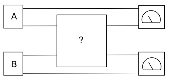
Figure 1: Schematic of the operational scenario for channel certification.

II.2 Notation

In this work, we will encounter two families of well-known quantum channels. In order to set notation, we mention them here briefly. The first family are the unitary channels, which will be denoted

$$\Psi_{U}(\rho)=U\rho U^{\dagger},$$ (1)

as an input state $\rho$ and a unitary matrix $U$.

The second family are von Neumann measurements, which are a special case of positive operator-valued measures (POVMs). In a finite-dimensional case, a POVM can be represented by a set of positive semi-definite operators $P=\{E_{m}\}_{m}$, such that $\sum_{m}E_{m}=\mathbb{I}$ and for a given state $\rho$ the probability of obtaining the measurement outcome $m$ is $p_{m}=\Tr\rho E_{m}$. Von Neumann’s measurements fulfil the additional requirement that all matrices $E_{m}$ are rank-one projectors. Hence, for a von Neumann measurement acting on a state of dimension, $d$ there are exactly $d$ matrices $E_{m}$ which are pairwise orthogonal. This simple observation allows us to parametrize a $d$ dimensional von Neumann measurement using a unitary matrix $U$

$$P_{U}=\{U\outerproduct{i}{i}U^{\dagger}\}_{i=1}^{d}.$$ (2)

As a shorthand notation, we will write $\ket{u_{i}}\mathrel{\vbox{\hbox{\scriptsize.}\hbox{\scriptsize.}}}=U\ket{i}$. We can associate a measure-and-prepare channel with a von Neumann measurement

$$P_{U}(\rho)=\sum_{i=1}^{d}\bra{u_{i}}\rho\ket{u_{i}}\outerproduct{i}{i}.$$ (3)

II.3 Numerical ranges of a matrix

In the context of certifying unitary states and channels, the numerical range and the $q$-numerical range play a pivotal role. The numerical range of a square matrix $X$ of size $d$, is defined as a subset of the complex plane:

$$W(X)=\{\bra{\psi}X\ket{\psi}:\innerproduct{\psi}{\psi}=1\},$$ (4)

where $X$ is some square matrix. The set $W(X)$ is compact and convex, an in depth discussion of its properties can be found in Fiedler (1981). Use of this structure in the context of quantum states is described in Dunkl et al. (2011).

The set $q$-numerical range is defined as:

$$\begin{split}W_{q}(X)&=\{\bra{\psi}X\ket{\phi}:\innerproduct{\psi}{\phi}=q,\\ &\phantom{{}={}}\innerproduct{\psi}{\psi}=1,\innerproduct{\phi}{\phi}=1\},\end{split}$$ (5)

where $q$ is a complex number. The fundamental properties of such sets, along with a method for generating them, can be found in Li and Nakazato (1998). In Appendix A we present an easy way to produce vectors of given scalar product.

Based on these considerations, we can introduce the notions of product numerical ranges. First, let us define the product numerical range:

$$\begin{split}W^{\otimes}(X)&=\{(\bra{\psi_{1}}\otimes\bra{\psi_{2}})X(\ket{\psi_{2}}\otimes\ket{\psi_{1}}):\\ &\phantom{{}={}}\innerproduct{\psi_{1}}{\psi_{1}}=1,\innerproduct{\psi_{2}}{\psi_{2}}=1\}.\end{split}$$ (6)

The core properties of this object are described in Puchała et al. (2011). Additionally, we introduce a new structure, which to the best of our knowledge, hasn’t been defined in literature yet. However, based on the previous definitions, it represents a natural extension of the $q$-numerical range. The product $q$-numerical range is defined as:

$$\begin{split}W_{q}^{\otimes}(X)&=\{(\bra{\psi_{1}}\otimes\bra{\psi_{2}})X(\ket{\phi_{2}}\otimes\ket{\phi_{1}}),\\ &\phantom{{}={}}\innerproduct{\psi_{1}}{\phi_{1}}\innerproduct{\psi_{2}}{\phi_{2}}=q,\text{ and for }i=1,2\\ &\phantom{{}={}}\innerproduct{\psi_{i}}{\psi_{i}}=1,\innerproduct{\phi_{i}}{\phi_{i}}=1\}.\end{split}$$ (7)

II.4 Examples of product $q$-numerical ranges

The main result of this study is described using the product $q$-numerical range; thus, we will focus on this structure. We examine sets generated for an operator acting in a complex space of dimension $d=4$. For presentation, we chose the matrix $U$ of type:

$$U(\theta)=V(\theta)DV^{\dagger}(\theta),$$ (8)

where $D$ is a diagonal matrix containing the eigenvalues, and V is a unitary matrix depending on one parameter

$$V(\theta)=\begin{pmatrix}\cos(\theta)&0&0&\sin(\theta)\\ 0&\frac{1}{\sqrt{2}}&\frac{1}{\sqrt{2}}&0\\ 0&\frac{1}{\sqrt{2}}&\frac{-1}{\sqrt{2}}&0\\ -\sin(\theta)&0&0&\cos(\theta)\end{pmatrix}$$ (9)

The product state appearing in the definition of product numerical range can be equated with the product of two qubits. The numerical range and the $q$-numerical range has an essential property: their plot is a convex set. However, this property is lost for their product counterparts. Example representations of the product $q$-numerical range are presented in Figures 2, 3.

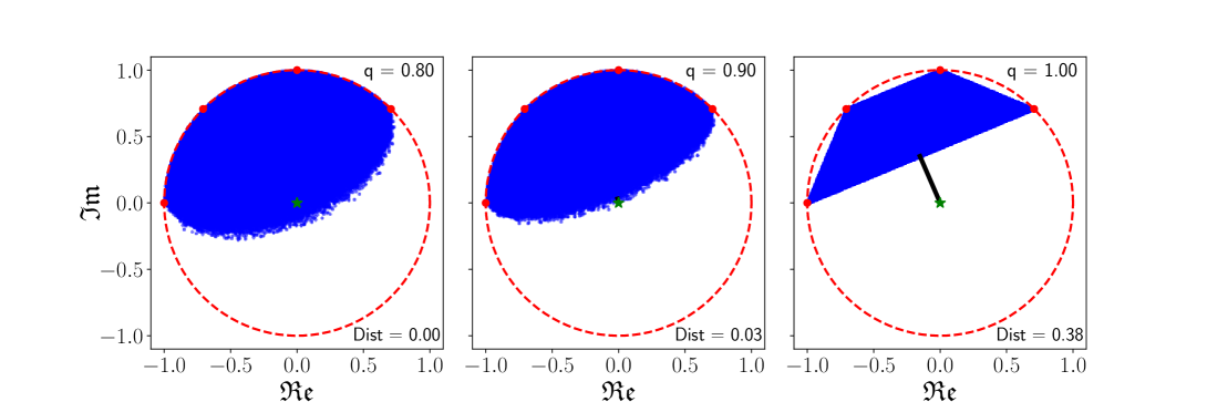
Figure 2: $q$-numerical range of the matrix $U\left(\frac{\pi}{8}\right)$ from Eq. (8) with distance from the origin. The red dots are the eigenvalues of $U\left(\frac{\pi}{8}\right)$.

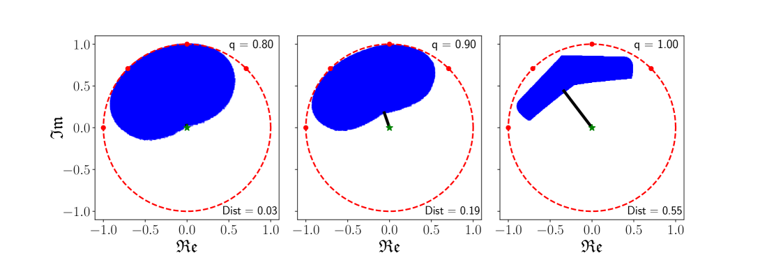
Figure 3: Product $q$-numerical range of the matrix $U\left(\frac{\pi}{8}\right)$ from Eq. (8) with distance from the origin. The red dots are the eigenvalues of $U\left(\frac{\pi}{8}\right)$.

III Main results

We considered the problem of certifying unknown quantum operations by two parties, Alice and Bob. In our case, the unknown operation will be either a unitary channel or a von Neumann measurement. Each of the parties involved can prepare an arbitrary input state. Our goal is to determine or set a limit on the probability of a type II error in hypothesis testing.

• $H_{0}$: The operation is $\Phi_{0}$.

• $H_{1}$: The operation is $\Phi_{1}$.

In our case we assume without loss of generality that $\Phi_{0}=\Psi_{\mathbb{I}}$ ($\Phi_{0}=P_{\mathbb{I}}$) and $\Phi_{1}=\Psi_{U}$ ($\Phi_{1}=P_{U}$) for the case of certification of unitary channels (von Neumann measurements).

As per Fig. 1 each of the parties can prepare a general, possibly entangled input state, whose part will be subjected to the certified operation. Then, each party can perform a measurement on their entire system. The measurement is assumed to be binary and, in the case of measurement, certification may be conditioned on the obtained output. Hence, the measurement available is $\left\{\Omega_{1}\otimes\Omega_{2},\mathbb{I}-\Omega_{1}\otimes\Omega_{2}\right\}$. If, as a result, the label corresponding to $\Omega_{1}\otimes\Omega_{2}$ is obtained, we accept the null hypothesis, otherwise we reject it. In our setting, we assumed, without loss of generality, that the parties do not reject a hypothesis $H_{0}$, if they both obtain a given outcome and reject it otherwise. Thus, we arrive at the following formulas for the probabilities of type I and type II errors:

$$\begin{split}p_{I}(\Omega_{1}\otimes\Omega_{2},\ket{\psi_{1}}\otimes\ket{\psi_{2}})=&\mathrm{Tr}\left((1-\Omega_{1}\otimes\Omega_{2})(\Phi_{0}\otimes\mathbb{I})(\ket{\psi_{1}}\otimes\ket{\psi_{2}}\bra{\psi_{2}}\otimes\bra{\psi_{1}})\right)=\\ =&1-\mathrm{Tr}\left(\Omega_{1}\otimes\Omega_{2}(\Phi_{0}\otimes\mathbb{I})(\ket{\psi_{1}}\otimes\ket{\psi_{2}}\bra{\psi_{2}}\otimes\bra{\psi_{1}})\right).\end{split}$$ (10)

$$p_{II}(\Omega_{1}\otimes\Omega_{2},\ket{\psi_{1}}\otimes\ket{\psi_{2}})=\mathrm{Tr}\left(\Omega_{1}\otimes\Omega_{2}(\Phi_{1}\otimes\mathbb{I})(\ket{\psi_{1}}\otimes\ket{\psi_{2}}\bra{\psi_{2}}\otimes\bra{\psi_{1}})\right).$$ (11)

Certification requires minimizing $p_{II}$ the subject under the condition $p_{I}\leq\delta$, where $\delta$ is the desired significance level:

$$p_{II}=\min_{\ket{\psi_{1}}\otimes\ket{\psi_{2}}}\min_{(\Omega_{1}\otimes\Omega_{2}:p_{I}(\Omega_{1}\otimes\Omega_{2},\ket{\psi_{1}}\otimes\ket{\psi_{2}})\leq\delta)}p_{II}(\Omega_{1}\otimes\Omega_{2},\ket{\psi_{1}}\otimes\ket{\psi_{2}}).$$ (12)

The first minimum ensures the appropriate significance level, while the second ensures that parties A and B operate optimally. Therefore, one should find the optimal $\ket{\psi_{0}}=\ket{\psi_{1}}\otimes\ket{\psi_{2}}$ and $\Omega_{0}=\Omega_{1}\otimes\Omega_{2}$ that satisfy:

$$\mathrm{Tr}\left(\Omega_{0}(\Phi_{0}\otimes\mathbb{I})(\ket{\psi_{0}}\bra{\psi_{0}})\right)\geq 1-\delta.$$ (13)

III.1 Unitary channel certification

Given two available unitary channels, without loss of generality, one can assume that one of them is the identity. Therefore, the channels have the form $\Psi_{\mathbb{I}},\Psi_{U}$. The remainder of this section is devoted to proving the following theorem. This result shows the relation between two-party certification and the product $q$-numerical range.

Theorem 1.

Consider the problem of two-point local certification of quantum channels with hypotheses given by:

$$\begin{split}H_{0}&=\Psi_{\mathbb{I}}\otimes\mathbb{I};\\ H_{1}&=\Psi_{U}\otimes\mathbb{I},\end{split}$$ (14)

where the systems are as in Fig. 1. Taking the most powerful test with product measurement, the probability of the type II error yields

$$p_{II}=\min\limits_{q\geq\sqrt{1-\delta}}(W_{q}^{\otimes}(U\otimes\mathbb{I}))^{2}.$$ (15)

Proof.

The possibility of choosing pure effects $\Omega_{1}$ and $\Omega_{2}$ follows from simple convex analysis. Note that if we fix $\Omega_{1}$ we encounter the standard certification scenario, and in this case, it is known that one can choose pure effect $\Omega_{2}=\ket{\omega_{2}}\bra{\omega_{2}}$, see e.g.  Lewandowska et al. (2021b). By repeating this procedure, we see that one can always choose a pure effect for both parties to obtain the optimal certification scheme. Similarly, we can show, that parties can restrict themselves to using only pure input states. Hence, the measurements are both product and von Neumann in nature, they can be represented as:

$$\Omega_{1}\otimes\Omega_{2}=\ket{\omega_{1}}\bra{\omega_{1}}\otimes\ket{\omega_{2}}\bra{\omega_{2}}.$$ (16)

The condition for the type I error is then formulated as:

$$p_{I}(\Omega_{1}\otimes\Omega_{2},\ket{\psi_{1}}\otimes\ket{\psi_{2}})\\ =\mathrm{Tr}\left(1-\Omega_{1}\otimes\Omega_{2}(\Psi_{\mathbb{I}}\otimes\mathbb{I})\ket{\psi_{1}}\bra{\psi_{1}}\otimes\ket{\psi_{2}}\bra{\psi_{2}}\right)\\ =1-\left|\innerproduct{\omega_{1}}{\psi_{1}}\innerproduct{\omega_{2}}{\psi_{2}}\right|^{2}\leq\delta.$$ (17)

The final form of the condition under which we minimize is given by:

$$\left|\innerproduct{\omega_{1}}{\psi_{1}^{R}}\innerproduct{\omega_{2}}{\psi_{2}^{R}}\right|^{2}\geq 1-\delta.$$ (18)

Hence, the condition for optimizing the type II error is:

$$\begin{split}p_{II}&=\min_{\ket{\psi_{1}^{R}}\otimes\ket{\psi_{2}^{R}}}\min_{(\Omega_{1}\otimes\Omega_{2}):p_{I}((\Omega_{1}\otimes\Omega_{2}),\ket{\psi_{1}^{R}}\otimes\ket{\psi_{2}^{R}})\leq\delta}\mathrm{Tr}\left(\Omega_{1}\otimes\Omega_{2}(\Phi_{U}\otimes\mathbb{I})(\ket{\psi_{1}^{R}}\bra{\psi_{1}^{R}})\otimes\ket{\psi_{2}^{R}}\bra{\psi_{2}^{R}}\right)=\\ &=\min_{\ket{\psi_{1}^{R}},\ket{\psi_{2}^{R}},\ket{\omega_{1}},\ket{\omega_{2}}:\left|\innerproduct{\omega_{1}}{\psi_{1}^{R}}\innerproduct{\omega_{2}}{\psi_{2}^{R}}\right|^{2}\geq 1-\delta}\mathrm{Tr}\left(\ket{\omega_{1}}\bra{\omega_{1}}\otimes\ket{\omega_{2}}\bra{\omega_{2}}(U\otimes 1)(\ket{\psi_{1}^{R}}\bra{\psi_{1}^{R}}\otimes\ket{\psi_{2}^{R}})\bra{\psi_{2}^{R}}\right)=\\ &=\min_{\ket{\psi_{1}^{R}},\ket{\psi_{2}^{R}},\ket{\omega_{1}},\ket{\omega_{2}}:\left|\innerproduct{\omega_{1}}{\psi_{1}^{R}}\innerproduct{\omega_{2}}{\psi_{2}^{R}}\right|\geq\sqrt{1-\delta}}|\bra{\psi_{1}^{R}}\otimes\bra{\psi_{2}^{R}}U\otimes 1\ket{\omega_{1}}\otimes\ket{\omega_{2}}|^{2}.\end{split}$$ (19)

Then, the result 15 is straightforward. ∎

For $q$-numerical range, the following two properties hold Duan et al. (2009):

$$\min{W_{q^{\prime}}(X)}\geq\min{\frac{q^{\prime}}{q}W_{q}(X)},\hskip 14.22636ptq<q^{\prime}\in\mathbb{R}.$$ (20)

$$W_{q}(X)=W_{q}(X\otimes\mathbb{I}).$$ (21)

Numerical simulations of dimension $d=8$ suggest that these properties also hold for the set of product numerical $q$-range. Based on this conjecture, we could replace the inequality sign with equality in equation (15). Furthermore, the extension by identity could be removed and Eq. (15) could be rewritten as

$$p_{II}=\min\limits_{q=\sqrt{1-\delta}}(W_{q}^{\otimes}(U))^{2}.$$ (22)

taking equality instead of inequality is also an intuitively expected result, as increasing the maximum type I error should reduce the type II error. If this were not the case, somewhere beyond zero, there would be an area where increasing the maximum type II error would not result in a reduction in type I error. For further details, refer to the visualizations in Appendix B.

III.2 Von Neumann measurement certification

In this section, we extend the framework of quantum measurement certification to focus on the local certification of von Neumann measurements. Drawing upon the foundational principles introduced in Lewandowska et al. (2021b), our primary objective is to certify a specific measurement, denoted as $P_{\mathbb{I}}$, under the alternative hypothesis $P_{U}$. Again, without loss of generality, we assume that one measurement can be performed in the computational basis. In alignment with the original work, we leverage the measure-and-prepare channel paradigm to facilitate the certification process. This approach allows us to associate each quantum measurement with a corresponding measure-and-prepare channel, thereby providing a robust framework for local certification.

We summarize our findings with the following theorem:

Theorem 2.

Consider the problem of two-point local certification of von Neuman measurements with hypotheses given by:

$$\begin{split}H_{0}&=P_{\mathbb{I}}\otimes\mathbb{I};\\ H_{1}&=P_{U}\otimes\mathbb{I},\end{split}$$ (23)

For the most powerful test, the probability of the type II error can be bounded by:

$$p_{II}\geq\max_{E\in DU_{d}}(\min_{q\geq\sqrt{1-\delta}}(W^{\otimes}_{q}((UE)^{\dagger}\otimes\mathbb{I}))^{2}.$$ (24)

Proof.

Start from the observation that each von Neumann measurement $P_{U}$, can be expressed as $\Delta\circ\Phi_{{(UE)}^{{\dagger}}}$. Here, $\Delta$ is the completely dephasing channel $\Delta(X)=\sum_{i}\bra{i}X\ket{i}\outerproduct{i}{i}$, $E$ is a diagonal unitary matrix Lewandowska et al. (2021a).

By utilizing the inequality delivered in Lemma 1 in Lewandowska et al. (2021a), followed by the result from the local channel certification [Eq. (III.1)] we obtain:

$$\begin{split}p_{II}&\geq\min_{\ket{\psi_{1}^{R}}\otimes\ket{\psi_{2}^{R}}}\min_{(\Omega_{1}\otimes\Omega_{2}):p_{I}((\Omega_{1}\otimes\Omega_{2}),\ket{\psi_{1}^{R}}\otimes\ket{\psi_{2}^{R}})\leq\delta}\mathrm{Tr}\left(\Omega_{1}\otimes\Omega_{2}(\Phi_{(UE)^{\dagger}}\otimes\mathbb{I})(\ket{\psi_{1}^{R}}\bra{\psi_{1}^{R}})\otimes\ket{\psi_{2}^{R}}\bra{\psi_{2}^{R}}\right)=\\ &=\min_{q\geq\sqrt{1-\delta}}(W^{\otimes}_{q}((UE)^{\dagger}\otimes\mathbb{I}))^{2}\end{split}$$ (25)

Maximizing over $E$ leads to the lower bound of the form (24). ∎

IV Summary

In this work, we considered a scenario in which two parties with access to a common channel undertake its certification. After using the channel, they each make a separate measurement on their respective systems. To analyze this approach, we introduced a product version of the $q$-numerical range and examined certain properties expressed by formulas (20), (21). We focused our studies on two classes of channels to be certified: unitary channels and von Neumann measurements. In case of unitary channels, we showed that this problem can be reduced to optimization on the product $q$-numerical range. In the case of von Neumann measurements we showed that we gain partial information, specifically on lower bound of type II error.

Appendix A Algorithm for generating vectors with given scalar product

A significant component of the research on product $q$-numerical ranges is the capability to generate them numerically, enabling the analysis of examples. In the section, we provide an example algorithm that produces normalized vectors with a scalar product equal to $q$. Using well-established methods, we randomly choose a unitary matrix of the desired dimension. We pick the first two columns of this matrix, $\ket{u_{1}}$, $\ket{u_{2}}$. We aim to find a normalized vector $\ket{z}$ such that $\innerproduct{u_{1}}{z}=q$. Let us define,

$$\ket{z}=\frac{(\ket{u_{2}}+a\ket{u_{1}})}{\sqrt{1+|a|^{2}}},$$ (26)

From the condition above, we obtain the condition

$$a=\frac{q}{1-q^{2}}.$$ (27)

When $q=1$, we set $\ket{z}=\ket{u_{1}}$.

Appendix B Product $q$-numerical range visualization

The following figures illustrate the product $q$-numerical range of a unitary matrix $U$ defined in Eq. (8) parameterized by $\theta$ for various values of $q$.

The same result was obtained after adding an auxiliary identity channel to the simulation. Those results support the hypothesis that the result for channel certification 15 can be simplified by removing inequality for $q$ and entanglement assistance.

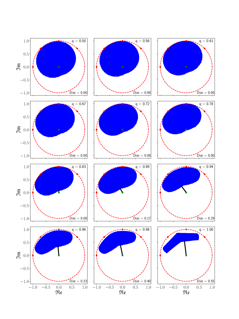
Figure 4: Product $q$-numerical range of the matrix $U\left(\frac{\pi}{8}\right)$ from Eq. (8) for ten values of $q$ from interval $[0.5,1]$. The range is represented in the complex plane, highlighting the non-convexity and the dependence on the parameter $q$. Each plot is accompanied by a calculated distance from the origin, indicating the minimum error probability in quantum hypothesis testing for the corresponding $q$ value. The non-convexity of these sets is a direct consequence of the product structure.

References

- Helstrom (1970) C. W. Helstrom, Journal of Statistical Physics 1, 231 (1970).
- Emmert-Streib and Dehmer (2019) F. Emmert-Streib and M. Dehmer, Machine Learning and Knowledge Extraction 1, 945 (2019).
- Gawron et al. (2010) P. Gawron, Z. Puchała, J. A. Miszczak, Ł. Skowronek, and K. Życzkowski, Journal of Mathematical Physics 51, 102204 (2010).
- Lewandowska et al. (2021a) P. Lewandowska, A. Krawiec, R. Kukulski, Ł. Pawela, and Z. Puchała, Scientific reports 11, 1 (2021a).
- Fiedler (1981) M. Fiedler, Linear Algebra and its Applications 37, 81 (1981).
- Dunkl et al. (2011) C. F. Dunkl, P. Gawron, J. A. Holbrook, J. A. Miszczak, Z. Puchała, and K. Życzkowski, Journal of Physics A: Mathematical and Theoretical 44, 335301 (2011).
- Li and Nakazato (1998) C.-K. Li and H. Nakazato, Linear and Multilinear Algebra 43, 385 (1998).
- Puchała et al. (2011) Z. Puchała, P. Gawron, J. A. Miszczak, Ł. Skowronek, M.-D. Choi, and K. Życzkowski, Linear Algebra and its Applications 434, 327 (2011).
- Lewandowska et al. (2021b) P. Lewandowska, A. Krawiec, R. Kukulski, Ł. Pawela, and Z. Puchała, Scientific Reports 11 (2021b), 10.1038/s41598-021-81325-1.
- Duan et al. (2009) R. Duan, Y. Feng, and M. Ying, Physical Review Letters 103, 210501 (2009).