On Density Functional Theory models for one-dimensional homogeneous materials
Abstract.
This paper studies DFT models for homogeneous 1D materials in the 3D space. It follows our previous work about DFT models for homogeneous 2D materials in 3D. We show how to reduce the problem from a 3D energy functional to a 2D energy functional. The kinetic energy is treated as in [7, 8] by diagonilizing admissible states, and writing the kinetic energy as the infimum of a modified kinetic energy functional on reduced states. Besides, we treat here the Hartree interaction term in 2D, and show how to properly define the mean-field potential, through Riesz potential. We then show the well posdness of the reduced model and present some numerical illustrations.
1. Introduction
In recent years, low-dimensional materials, such as 2D sheets, 1D nanowires and quantum dots have become of great importance in condensed matter physics due to their distinctive features, which are relevant in many applications [6, 19, 22, 3, 9, 1, 26]. In order to investigate their electronic properties, such as electron’s mobility and band gap, Density Functional Theory (DFT) calculations are often used [4, 24, 11, 18, 20, 25]. Our objective is to prove and study DFT models for low-dimensional systems in order to allow low computational cost. In [2], the Thoma-Fermi-von Weisäcker model for 1D and 2D materials is derived by means of thermodynamic limit procedure. The works [7, 8] have initiated the study of DFT models for low dimensional materials that are homogeneous, and we were particularly interested in 2D materials embedded in the 3D space. In this paper, we focus on one–dimensional materials that have an atomic length in two dimensions of the space, and a crystalline structure in the remaining dimension.
In [7], 2D materials are considered with a nuclear charge distribution of the form
that depends only on the orthogonal direction . The electrons are described by one body density matrices that satisfy Pauli principle . As the problem is convex, share the same symmetry as ,
| (1.1) |
where is the translation operator along the first two variables. Note that the density associated to a satisfying (1.1) depends only on the third variable and the trace per unit surface of can be defined by . In the reduced Hartree-Fock (rHF) model, the energy of the system is of the form
where denotes the the Laplacian operator on , and is the 1D Hartree interaction. One main result of [7] is a thorough discussion of this term and the definition of the mean-field potential (see [7, Proposition 3.3]). We prove that this problem is equivalent to a one-dimensional problem set on operators acting on , which are positive , but which no longer need to satisfy Pauli principle. Instead, an additional term appears in the energy: the three-dimensional kinetic energy is replaced by a one-dimensional kinetic energy of the form
Although we restrict ourselves to the reduced Hartree-Fock model for simplicity, similar derivations can be performed for general Kohn–Sham models and one can consider models of the form
In [8], we have considered a uniform magnetic field which is perpendicular to the 2D material axis. The reduction here is obtained considering operators commuting with magnetic translations. We first provide a decomposition of such operators and then state the equivalent one-dimensional problem in which the kinetic energy per unit surface has been repalaced by
where denotes the three-dimensional Landau operator, the magnetic field strenghten, and a suitable piecewise linear function, see for instance [8, Theorem 3.1].
In the present paper, we consider homogeneous 1D materials, i.e. nuclear charge distributions of the form
that do not depend on the third variable , the axis of the material. As we consider convex models, we assume that the electronic density matrices follow the same symmetries
| (1.2) |
where denotes the translation operator by the vector . Again, states satisfying the symmetry (1.2) have densities that depend only on and and the trace per unit length of can be defined by . In the reduced Hartree-Fock model, the energy of the system is
| (1.3) |
where is the 2D Hartree interaction. Formally, the interaction term is defined by
| (1.4) |
This definition is only valid for functions that decay fast enough at infinity. Besides, it is unclear whether this bilinear form is bounded from below or not. One key result of this paper is a regularization of this expression adapted to neutral systems; and a definition of the corresponding mean-field potential (see Section 2).
For the kinetic part, following the same arguments as in [7], we prove that this problem is equivalent to a two-dimensional problem, where the three-dimensional kinetic energy is replaced by a two-dimensional kinetic energy of the form
defined on . The reduced 2D rHF energy then reads
| (1.5) |
We show that this problem of minimizing the energy (1.5) over a suitable set of admissible states admits a unique minimizer, called ground state. We also derive the self-consistent equation that this ground state needs to satisfy.
Finally, we perform numerical simulations on the simpler Thomas–Fermi model, where the kinetic energy is expressed as an explicit functional of the density . This allows us to exhibit the properties of the regularized 2D Hartree interaction with respect to the classical expression (1.4).
This article is organized as follow. Section 2 is devoted to the regularization of the 2D Hartree interaction and the definition of the corresponding mean-field potential. In Section 3, we show how to reduce the 3D problem (1.3) into the 2D model (1.5), that we study in Section 4. Finally, in Section 5, we consider the orbital free Thomas-Fermi model as a semi–classical limit of the rHF model in order to perform elementary numerical illustrations.
Acknowledgments. The research leading to these results has received funding from OCP grant AS70 “Towards phosphorene based materials and devices”. S. Lahbabi thanks the CEREMADE for hosting her during the final writing of this article.
2. 2D Hartree interaction
For 1D crystals, the Hartree interaction kernel has been derived in [2] by means of thermodynamic limit procedure. It is given by
and the Hartree interaction energy is formally given by
where . For functions which do not depend on the third variable , this interaction reduces to
| (2.1) |
The integral in (2.1) is only valid for functions decaying fast enough and the map is not convex in general. The aim of this section is to give a regularization of this expression suitable for neutral charge distributions, which, in our context, will be . We therefore adopt the following definition
| (2.2) |
where and belong to the following Coulomb space
We have denoted by the Fourier transform in defined by . We note that the integrability of over implies that
which means that elements of are neutral distributions. Conversely, for neutral distributions that decay fast enough, and coincide.
Lemma 2.1.
If is such that and , then
The proof of this lemma can be found in [5].
For , let us introduce as
Thanks to Parseval identity, one can rewrite the interaction as
An explicit expression of , for , is given through the Riesz potential as follows (see for instance [23, Chapter V]).
Lemma 2.2.
Let . Then,
| (2.3) |
The integral in (2.3) is absolutely convergent whenever , for some (see for instance [23, Theorem 1 of Chapter V]). Furthermore, if and . Then,
| (2.4) |
for a suitable constant which is independent of .
We turn now to the definition of a mean-field potential associated to a charge distribution . It needs to satisfy
and
in a weak sense. One would consider . However, the integral in (2.3) is not necessarily convergent in the critical case of . We suggest an alternative way to define the potential , for through a modification of the Riesz potential suggested in [13]. Let us define the following two functions
where
In the following proposition, we define and state some properties of the modified Riesz potential. For the proof and further details, we refer to [13, Corollary 3.23].
Proposition 2.3.
For , define
| (2.5) |
One has the following
-
a)
and are well-defined, i.e., the integrals in (2.5) are convergent.
-
b)
There exist two real numbers and such that
(2.6)
As a consequence of Proposition 2.3, we have , for . Now, for , we define the mean field potential as
| (2.7) |
The following theorem is one of the main results of the paper and it allows to rewrite the potential energy in terms of the mean–field potential .
Theorem 2.4.
Let . Then
| (2.8) |
and satisfies
| (2.9) |
in a distributional sense.
Proof.
Let us first prove (2.8) for in the Schwartz space of fast decaying functions . Since , for . Then, one can write
| (2.10) |
In order to apply Fubini theorem and change the order of the integrals in the above double intgrals, we have to check the absolute integrability. Regarding the first term, one can note that is in , thanks to (2.6), and so is . Therefore, one has
| (2.11) |
Taking into the account that the estimate in (2.6) holds true if one substitutes the kernel defining by its absolute value (see for instance [13, Theorem 3.19]), then the last double intergal of (2) is absolutely convergent as well. Thus,
| (2.12) |
By adding (2.11) et (2.12), we obtain
Now, let . Then, and . By density of the Schwartz space , one can find with such that in and in . Hence, one obtains (2.8), for , by letting .
We move now to the proof of (2.9). If one denotes by the distributional brakets, then, for ,
One knows that satisfies . Thus, by the previous result
∎
3. Model reduction
In this section, we show that the 3D reduced Hartree Fock model for homogeneous 1D crystal is equivalent to a 2D model. Other DFT models can be handled similarly. We recall that the nuclear charge distribution satisfies
| (3.1) |
We assume that the charge per unit length is finite, that is,
In Hartree–Fock type models, the state of electrons is described by a bounded self–adjoint operator satisfying Pauli exclusion principle . In our particular case, the system has the following features.
-
•
It is equidistributed in one direction of the three–dimensional space,
-
•
it is confined in the remaining two directions with a finite number of particles.
The electronic states share the aforementioned invariance as follows
| (3.2) |
where denotes the translation operator by the vector (). The 3D rHF energy of a state in
is
where we have denoted by the space of self–adjoint, locally trace class operators acting on , and is the regularized 2D Hartree interaction introduced in the previous section. We now define the 2D energy functional for a state in
| (3.3) |
where we have denoted by the space of self–adjoint, trace class operators acting on , by
| (3.4) |
The main result of the section is the following theorem.
Theorem 3.1.
The ground state energies
and
| (3.5) |
are equal and the minimizers of both energies share the same densities, which does not depend on .
The proof of theorem (3.1) follows the same line as the one of [7, Theorem 2.8]. We highlight here some arguments in the 2D case.
Diagonalization of admissible states. We start by showing that states in can be diagonalized. Let us introduce the partial Fourier transform
where refers to the Fourier transform in . According to the Floquet–Bloch decomposition (see [21, Section XIII–16]), for any there exists a unique family of self–adjoint operators on , called the fibers of , such that
| (3.6) |
that is, for any ,
We point out that, if , then its fibers satisfy Pauli principle . The following proposition links other properties of to those of its fibers.
Proposition 3.2.
Let and suppose that is locally trace class. One has
-
•
admits an integral kernel and
(3.7) where, for every , is the integral kernel of .
-
•
Let denote the density of , given by for all . Then,
where refers to the density of .
In particular, does not depend on the third variable . -
•
The trace per unit length of is given by
Proof.
Diagonalization of the kinetic energy Let . Let such that is smooth enough for any . Straightforward computation yields
Hence, the kinetic energy per unit length of can be written
Reduced states Now, we map any admissible state to a reduced 2D state as follows
We notice that elements of , unlike those of , are compact operators. We have the following result.
Proposition 3.3.
The map is onto. Furthermore, for any ,
Proof.
Let . One can write , with an orthonormal family in and such that . We construct satisfying through its fibers . Let us define, for any , as
where, for any , will be determined later. One has and . Thus, . Moreover, . Therefore,
Finally, with the choice , one obtains , which proves the claim. ∎
Reduction of the kinetic energy We now rewrite the kinetic energy as a functional of elements of .
Theorem 3.4.
Let . Then,
| (3.8) |
Proof.
Remark 3.5.
A consequence of Theorem 3.4 is that for a representable charge density , one could associate the kinetic energy functional as follows
| (3.10) |
Finding an explicit expression for the above functional is highly challenging. It is only possible to associate a lower bound to this energy as follows
| (3.11) |
for an appropriate constant . This is a consequence of the Lieb–Thirring inequality, see for instance [15, 16] and [7, Appendix A] (see Section 5.1). In particular, this yields that , once the kinetic enegry of is finite. Actually, the two dimensional Lieb–Thiring inequality applied to implies that and the Hoffman-Ostenhof inequality claims that , see [10].
4. Well-posdness of the reduced model
This section is devoted to the analysis of the reduced two-dimensional problem (3.5). In particular, we prove well-posdness and show that the ground state satisfies a self-consistent equation.
Theorem 4.1.
Assume that . Then the energy in (3.4) admits a unique minimizer in . Furthermore, one has
| (4.1) |
where , for and should be unterstood in terms of functional calculus for the self–adjoint operator .
Proof.
The proof of this theorem follows the same lines as the one of [7, Theorem 2.8]. We detail here the main arguments in our 2D case. Existence and uniqueness of the minimizer. The set is convex and the functional is convex and positive. Then, the existence of a minimizer is reduced to the lower semi-continuity of . Let let be a minimizing sequence of and denote by . One has
where is a positive constant. In particular, and are bounded sequences in the Schatten space of trace class operators and is bounded in the Schatten space of cubic trace class operators . Hence, taking into the account that is closed, there exists such that
and
By the Lieb-Thirring inequality [15], is bounded in . Thus, converges weakly in . Moreover, its weak limit is . Indeed, for any function one has
where stands for the multiplication operator by in , and the convergence is obtained by the fact that is a compact operator. Besides, , for all . Hence,
Let us prove that . Let be a test function in the Schwartz space such that . By Parseval’s identity, one gets
Letting go to , and noting that , we obtain
This actually identifies with . Summarizing, one has and
which proves that is actually a minimizer of . The uniqueness comes from the strict convexity of .
Proof of the Euler Lagrange equation. Let denote the minimizer of , its density and the mean-field potential. Let and . One has and . Besides,
Thus,
Hence, dividing by and letting , one obtains
Proceeding as in [7, Sect. 4.3.2] and [8, Proposition 3.8], set and . Therefore, , for all . This implies that is bounded from below and
Set the bottom of the spectrum of . Then, . Next, let us expand as follows , where for any with , and . One has , for any such that . That is
Hence, belongs to the point spectrum of . Conversely, if such that , then is an eigenvalue of . This yields . Note that is a compact perturbation of ; thus they share the same essential spectrum. It follows that cannot have essential spectrum below . ∎
5. Numerical simulation
5.1. Thomas-Fermi model
We perform numerical illustrations on the simple Thomas-Fermi model, which can be seen as a semi–classical limit of the rHF model. The kinetic energy in this model reads
Therefore, for a given , we define the Thomas-Fermi energy per unit length as
for every , where
We point out that Thomas–Fermi model and its derivatives are widely considered in the literature, see [17, 12, 2]. The functional is stricltly convex and has a unique minimizer that satisifes the following self–consistent equation
| (5.1) |
with the Fermi level of the system is such that .
We emphasize that we still use our expression for the potential energy and the mean–field potential in (2.7) which is involved in the self–consistent equation (5.1). We next show a numerical solution to (5.1). We also contrast the outcomes from this equation with the non-regularized reduced energy in which the Coulomb energy and potential are
| (5.2) |
and
| (5.3) |
5.2. Numerical schemes
Python is used to carry out the numerical simulation. The two-dimensional functions are evaluated on a two-dimensional grid representing , with discretization points (we took and ). The various integrals inolved in the total energy are then approximated using quadrature techniques; we used the two-dimensional trapezoid rule.
We use two different methods in the regularized and non-regularized case. In the latter, the total energy is approximated using a numerical integration method. The constraints of the model are simply the positivity of the density along with the neutrality condition . The resulting discretized problem is thus a finite-dimensional optimization problem on (the approximated values of the density on the grid points) subject to linear constraints. This problem is solved numerically in Python using the predefined function minimize from Scipy library. In the regularized case, we apply an iterative process to solve equation (5.1) as follow: at each iteration , we evaluate the potential using (2.7) and we compute solution to
| (5.4) |
Note that, since is a non-decreasing function of , a simple dichotomy can be used to compute efficiently . We then update the density by setting
| (5.5) |
where is optimized to minimize the Thomas-Fermi energy (we use again the Python predefined function minimize). The algorithm is terminated when a tolerance is reached between two successively evaluated energies. We used .
For the approximation of the regularized energy by trapezoid rule, we use the formula (2.8) involving the potential, which is valid since is neutral, instead of the one involving the Fourier transform.
5.3. Numerical results
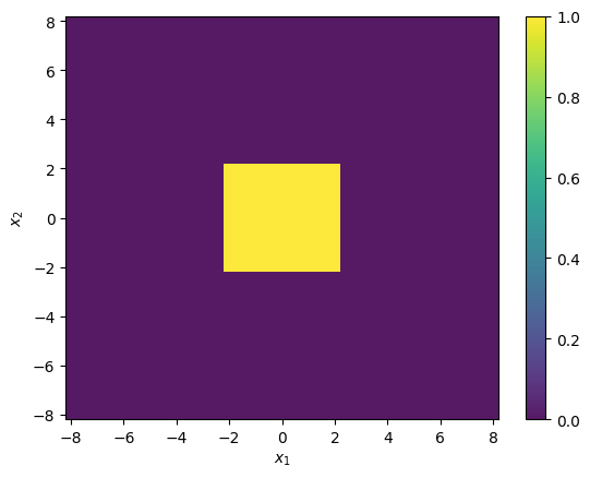
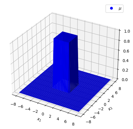
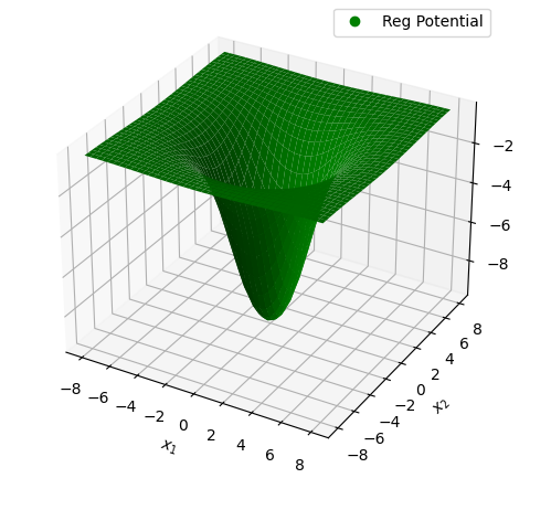
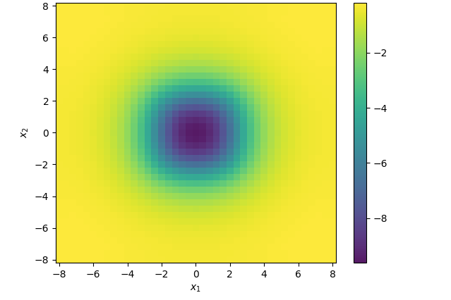
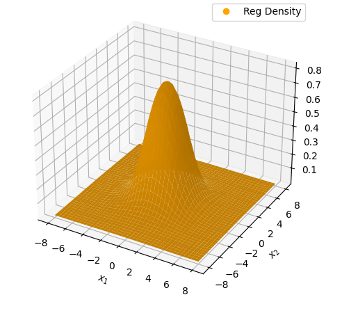
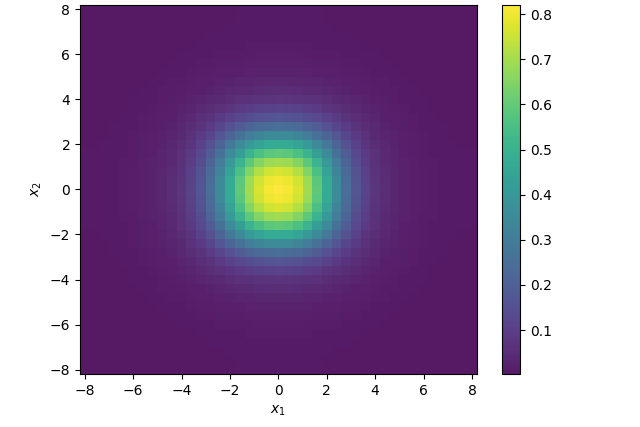
We present here the numerical results obtained for our test case, which corresponds to a homogeneous charged nanowire localized in a given square
| (5.6) |
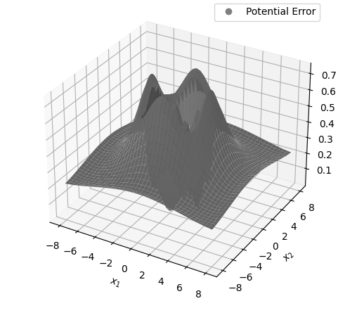
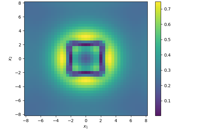
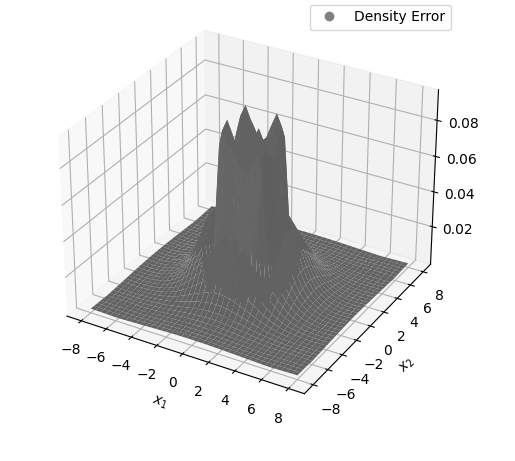
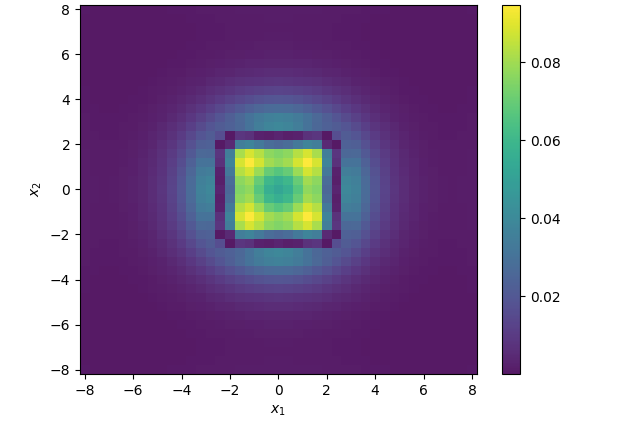
We note that we take . We start by plotting in Figure 1. Then, Figures 2 and 3 show the results for the non-regularized and regularized models, respectively. The two models’ combined results are fairly close. Figure 4 shows the error between the two models. We are able to say the following. The difference between the two densities appears to be almost zero far from the nanowire. The relative error is of order between potentials and of order between densities in the material’s vicinity. Ultimately, there is a error between the two ground states energies in the two models.
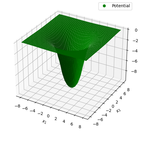

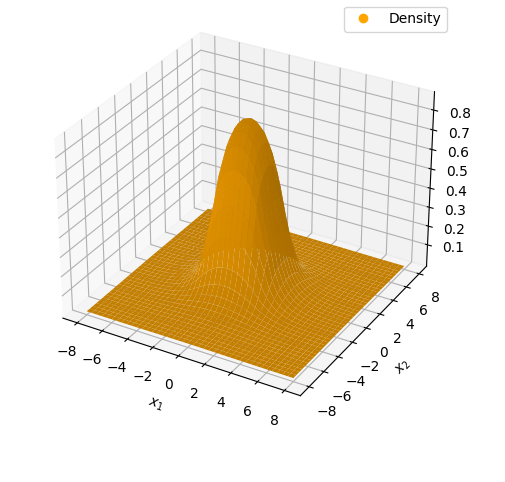

From a computational view point, the regularized model ends in 1902s with 13 iterations versus 2025s for the non-regularized model. Moreover, the energy obtained by the regularized model is lower than that of the non-regularized model (83,11 versus 89,46). More in-depth study remains to be done with finer grids and other test cases, but this first simple test allows to see the interest of the regularized model with respect to the non-regularized model, where there are no theoretical results for the existence and uniqueness of the minimizer.
References
- [1] A. A. Balandin, F. Kargar, T. T. Salguero, and R. K. Lake, One-dimensional van der waals quantum materials, Materials Today, 55 (2022), pp. 74–91.
- [2] X. Blanc and C. Bris, Thomas-Fermi type theories for polymers and thin films, Advances in Differential Equations, 5 (2000).
- [3] V. Chaudhary, P. Neugebauer, O. Mounkachi, S. Lahbabi, and A. EL Fatimy, Phosphorene - an emerging two-dimensional material: recent advances in synthesis, functionalization, and applications, 2D Materials, 9 (2022).
- [4] Y. Dai, W. Wei, Y. Ma, and C. Niu, Calculations and Simulations of Low-Dimensional Materials: Tailoring Properties for Applications, John Wiley & Sons, 2022.
- [5] L. Frerick, J. Müller, and T. Thomaser, A Fourier integral formula for logarithmic energy, ArXiv preprint, https://arxiv.org/abs/2209.05439, (2022).
- [6] A. Geim and I. Grigorieva, Van der Waals heterostructures, Nature, 499 (2013), pp. 419–425.
- [7] D. Gontier, S. Lahbabi, and A. Maichine, Density functional theory for two-dimensional homogeneous materials, Communication in Mathematical Physics, 388 (2021), pp. 1475–1505.
- [8] D. Gontier, S. Lahbabi, and A. Maichine, Density functional theory for two-dimensional homogeneous materials with magnetic fields, Journal of Functional Analysis, 285 (2023), p. 110100.
- [9] D. Gupta, V. Chauhan, and R. Kumar, A comprehensive review on synthesis and applications of molybdenum disulfide (mos2) material: Past and recent developments, Inorganic Chemistry Communications, 121 (2020), p. 108200.
- [10] M. Hoffmann-Ostenhof and T. Hoffmann-Ostenhof, "Schrödinger inequalities" and asymptotic behavior of the electron density of atoms and molecules, Phys. Rev. A, 16 (1977), pp. 1782–1785.
- [11] F. Hussain, D. Muhammad Imran, and H. U. Janjua, Density Functional Theory (DFT) Study of Novel 2D and 3D Materials, 07 2017, pp. 269–284.
- [12] P.-L. L. Isabelle Catto, Claude Le Bris, The Mathematical Theory of Thermodynamic Limits: Thomas–Fermi Type Models, Oxford Mathematical Monographs, Oxford University Press, USA, 1998.
- [13] T. Kurokawa, Riesz potentials, higher Riesz transforms and Beppo Levi spaces, Hiroshima Mathematical Journal, 18 (1988), pp. 541 – 597.
- [14] E. Lieb and Loss, Analysis, vol. 14 of Graduate studies in mathematics, American Mathematical Society, 2nd ed., 2001.
- [15] E. Lieb and W. Thirring, Bound on kinetic energy of fermions which proves stability of matter, Phys. Rev. Lett., 35 (1975), pp. 687–689.
- [16] , Inequalities for the moments of the eigenvalues of the Schrödinger hamiltonian and their relation to Sobolev inequalities, Studies in Mathematical Physics, Princeton University Press, 1976, pp. 269–303.
- [17] E. H. Lieb and B. Simon, The Thomas-Fermi theory of atoms, molecules and solids, Advances in Mathematics, 23 (1977), pp. 22–116.
- [18] H. Moustafa, Computational properties of one-dimensional materials, (2023).
- [19] Paras, K. Yadav, P. Kumar, D. R. Teja, S. Chakraborty, M. Chakraborty, S. S. Mohapatra, A. Sahoo, M. M. Chou, C.-T. Liang, et al., A review on low-dimensional nanomaterials: Nanofabrication, characterization and applications, Nanomaterials, 13 (2022), p. 160.
- [20] A. Patra, S. Jana, P. Samal, F. Tran, L. Kalantari, J. Doumont, and P. Blaha, Efficient band structure calculation of two-dimensional materials from semilocal density functionals, The Journal of Physical Chemistry C, 125,20 (2021), pp. 11206–11215.
- [21] M. Reed and B. Simon, Methods of Modern Mathematical Physics. Analysis of Operators, vol. IV, Academic Press, 1978.
- [22] J. Saha and A. Dutta, A review of graphene: Material synthesis from biomass sources, Waste and Biomass Valorization, 13 (2022).
- [23] E. M. Stein, Singular Integrals and Differentiability Properties of Functions, vol. 30 of Princeton Mathematical Series, Princeton University Press, 1970.
- [24] Q. Tang, Z. Zhou, and Z. Chen, Innovation and discovery of graphene-like materials via density-functional theory computations, WIREs Comput Mol Sci, 5 (2015).
- [25] H. Toffoli, S. Erkoç, and D. Toffoli, Modeling of nanostructures, (2012).
- [26] Z. Wang, T. Hu, R. Liang, and M. Wei, Application of zero-dimensional nanomaterials in biosensing, Frontiers in chemistry, 8 (2020), p. 320.