Quantum Weyl-Heisenberg antiferromagnet

Abstract

Beginning from the conventional square-lattice nearest-neighbor antiferromagnetic Heisenberg model, we allow the $J_{x}$ and $J_{y}$ couplings to be anisotropic, with their values depending on the bond orientation. The emergence of anisotropic, bond-dependent, couplings should be expected to occur naturally in most antiferromagnetic compounds which undergo structural transitions that reduce the point-group symmetry at lower temperature. Using the spin-wave approximation, we study the model in several parameter regimes by diagonalizing the reduced Hamiltonian exactly, and computing the edge spectrum and Berry connection vector, which show clear evidence of localized topological charges. We discover phases that exhibit Weyl-type spin-wave dispersion, characterized by pairs of degenerate points and edge states, as well as phases supporting lines of degeneracy. We also identify a parameter regime in which there is an exotic state hosting gapless linear spin-wave dispersions with different longitudinal and transverse spin-wave velocities.

I Introduction

More than three decades ago, Anderson proposed [1] that the large-amplitude quantum-spin fluctuations, present in the ground-state of the lowest-possible spin, the spin-1/2, Heisenberg antiferromagnet on the low-dimensional lattice, the square lattice, destroy the Néel order, and that the new emerging state of matter could be the foundation of the superconductivity observed in the cuprates. Subsequent work showed that the idea was not applicable to the spin-1/2 square lattice Heisenberg antiferromagnet [2]. However, Anderson’s proposal for the resonating-valence-bond state, whose original inception dates back nearly half a century [3], served as the ignition of a new field of research in “quantum magnetism”, aimed at realizing the quantum-spin liquid state. Most ensuing attempts to realize such states have focused on low-spin low-dimensionality systems, but they have departed from bi-partite lattices in an effort to introduce geometric frustration or frustrating interactions.

In the meantime, topology has emerged as a means of characterizing electronic structure [4], introducing new concepts and descriptions for condensed matter systems, such as the topological insulator [5, 6], the topological superconductor [7] and the Weyl semi-metal [8, 9]. Importing these ideas from topology into the field of quantum magnetism is a compelling pursuit for various reasons, including technological applications. For example, quantum spins may be used as the degrees of freedom in spintronics-magnonics applications [10] and in many proposals for quantum computing devices that require long coherence time-scales. Such long life-times are expected to be a fundamental property of topological quantum-spin states because of their inherently robust nature.

There are various ways to construct quantum-spin models furnishing topological characteristics. In this work, we focus on a model that exhibits quantum-spin Weyl behavior, an idea that has been explored in the literature in the context of various models. Quantum-spin Weyl behavior has been found in a pyrochlore antiferromagnet where a local spin anisotropic coupling [11, 12], allowed by the symmetry group, led to the emergence of Weyl magnons. Weyl magnons have also been discussed in the case of Honeycomb lattice ferromagnets [13] such as in CsI₃  [14]. Tunable topological magnon phases in triangular-honeycomb lattices have been studied [15] and also predicted [16] in layered ferrimagnets, where they arise as a result of spin-orbit coupling. Rather recently, an anomalous thermal Hall effect in the insulating van der Waals magnet VI₃ was observed [10], its existence attributed to topological magnons. Furthermore, it has been shown [17] that the addition of a second nearest-neighbor Dzyaloshinskii–Moriya interaction to the isotropic Heisenberg interaction can create Weyl magnons. Topological magnetic excitations have also been discussed [18] in the context of the Kitaev-Heisenberg model. Lastly, the general topological features of such bosonic models have also been discussed in the literature  [19].

In the present paper, we propose that such exotic, difficult-to-realize, models are not necessary to observe quantum-spin Weyl behavior. In fact, as we will show, this behavior is present in a slight (and known) modification of the familiar, garden-variety, spin-1/2 Heisenberg XYZ antiferromagnet on the square lattice! Beginning from the conventional square-lattice XYZ antiferromagnetic Heisenberg model, we introduce anisotropic couplings $J_{x}$ and $J_{y}$ whose values depend on the bond orientation. Within the spin-wave approximation, the effective bosonic model exhibits a Weyl-type spin-wave dispersion with edge states. The model is first investigated analytically, followed by a numerical investigation [20, 21] of the edge spectrum and Berry connection vector in various parameter regimes, which show clear evidence of localized topological charges. In short, we demonstrate that breaking the inversion symmetry introduces various interesting topological excitations of Weyl-boson character with topologically non-trivial edge states carrying topological charge.

Finally, we argue that such Weyl-magnon behavior, in perhaps the most basic model of magnetism, i.e., the nearest-neighbor Heisenberg antiferromagnet, with no additional terms, should be ubiquitous. We discuss how to experimentally realize such square-lattice quantum magnets endowed with the topological excitations and edge-states found here.

The paper is organized as follows. In the following section we introduce and analyze our model. In Sec. III we present our results and in Sec. IV we discuss our conclusions and how to realize the proposed behavior experimentally.

II Model

The Hamiltonian for the familiar $XYZ$ quantum Heisenberg antiferromagnet can be written as:

$$\hat{H}=\sum_{\alpha,\langle ij\rangle}J_{\alpha}(\boldsymbol{\delta}_{ij})\hat{S}^{\alpha}_{i}\hat{S}^{\alpha}_{j}-h\sum_{i=1}^{N}\hat{S}^{z}_{i},$$ (1)

where $\alpha=x,y,z$, $\boldsymbol{\delta}_{ij}$ is the vector connecting the nearest-neighbors $ij$, and $N$ is the number of sites. We will assume $J_{z}\geq J_{x},J_{y}$, and that there is $(\pi,\pi)$ antiferromagnetic order along the $z$ internal-spin direction. We define,

$$J_{\pm}(\boldsymbol{\delta}_{ij}) \equiv {{J_{x}(\boldsymbol{\delta}_{ij})\pm J_{y}(\boldsymbol{\delta}_{ij})}\over 2},$$ (2)

and introduce the spin-ladder operators,

$$\hat{S}^{x}_{i}={{\hat{S}^{+}_{i}+\hat{S}^{-}_{j}}\over 2},\hskip 14.45377pt\hat{S}^{y}_{i}={{\hat{S}^{+}_{i}-\hat{S}^{-}_{j}}\over{2i}},$$ (3)

with which the Hamiltonian can be rewritten in the following form:

$$\hat{H} = \sum_{{\bf R}\in A,\boldsymbol{\delta}}\left\{J_{z}\hat{S}^{z}_{\bf R}\hat{S}^{z}_{\bf R+\boldsymbol{\delta}}+{{1}\over 2}J_{+}(\boldsymbol{\delta})(\hat{S}^{+}_{\bf R}\hat{S}^{-}_{\bf R+\boldsymbol{\delta}}+\hat{S}^{-}_{\bf R}\hat{S}^{+}_{\bf R+\boldsymbol{\delta}})\right.$$ (4)

$$+ \left.{{1}\over 2}J_{-}(\boldsymbol{\delta})(\hat{S}^{+}_{\bf R}\hat{S}^{+}_{\bf R+\boldsymbol{\delta}}+\hat{S}^{-}_{\bf R}\hat{S}^{-}_{\bf R+\boldsymbol{\delta}})\right\}-h\sum_{i=1}^{N}\hat{S}^{z}_{i},$$

where we have introduced two sublattices, $A$ and $B$. The sum over $\bf R$ only includes sites on the $A$ sublattice, and the vector ${\boldsymbol{\delta}}=\pm a\hat{x},\pm a\hat{y}$ connects sites on the $A$ sublattice to sites on the $B$ sublattice. The sums over $\bf R$ and ${\boldsymbol{\delta}}$ therefore include all sites of the lattice.

Next, we carry out the well-known [2] substitution of the spin operators in terms of boson operators, $\hat{a}_{\bf{R}}$ ($\hat{a}_{\bf{R}}^{\dagger}$) and $\hat{b}_{\bf R}$ ($\hat{b}_{\bf R}^{\dagger}$) that destroy (create) spin fluctuations on the $A$ and $B$ sublattice respectively. Then, by expanding the Hamiltonian and keeping terms up to quadratic order in these boson operators we obtain:

$$\hat{H}_{LSW} = -{2N}S^{2}J_{z}+\varepsilon_{A}\sum_{{\bf R}\in A}^{N}\hat{a}^{\dagger}_{\bf R}\hat{a}_{\bf R}+\varepsilon_{B}\sum_{{\bf R}\in B}^{N}\hat{b}^{\dagger}_{\bf R}\hat{b}_{\bf R}$$ (5)

$$+ {J_{+}}S\sum_{{\bf R}\in A,\boldsymbol{\delta}}(\hat{a}_{\bf R}\hat{b}_{{\bf R}+\boldsymbol{\delta}}+\hat{a}^{\dagger}_{\bf R}\hat{b}^{\dagger}_{{\bf R}+\boldsymbol{\delta}})$$

$$+ S\sum_{{\bf R}\in A,\alpha}\left[v_{\alpha}(\hat{a}^{\dagger}_{\bf R}\hat{b}_{{\bf R}+\hat{\alpha}a}+\hat{a}_{\bf R}\hat{b}^{\dagger}_{{\bf R}+\hat{\alpha}a})\right.$$

$$\quad\quad+w_{\alpha}\left.(\hat{a}^{\dagger}_{\bf R}\hat{b}_{{\bf R}-\hat{\alpha}a}+\hat{a}_{\bf R}\hat{b}^{\dagger}_{{\bf R}-\hat{\alpha}a})\right],$$

where $\alpha=x,y$, the spin $S=1/2$, and we have taken $J_{z}$ and $J_{+}$ to be directionally-independent, i.e. $J_{z}(\boldsymbol{\delta})=J_{z}$, $J_{+}(\boldsymbol{\delta})=J_{+}$, and let $J_{-}(a\hat{x})=v_{x}$, $J_{-}(-a\hat{x})=w_{x}$, $J_{-}(a\hat{y})=v_{y}$, and $J_{-}(-a\hat{y})=w_{y}$. In addition we have defined, $\varepsilon_{A}\equiv 4SJ_{z}+h$, and $\varepsilon_{B}\equiv 4SJ_{z}-h$. An illustration of the terms of the Hamiltonian is shown in Fig.  1.

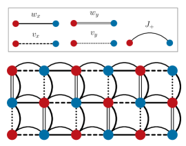
Figure 1: Illustration of lattice with coupling terms. Sublattice $A$ is denoted by the red circles, and sublattice $B$ by the blue circles. The box above the illustration indicates the line style corresponding to each coupling.

In momentum space we have,

$$\hat{H}_{\textrm{LSW}} =-{2N}S^{2}J_{z}+\varepsilon_{A}\sum_{\mathbf{k}}{\tilde{a}}^{\dagger}_{\mathbf{k}}{\tilde{a}}_{\mathbf{k}}+\varepsilon_{B}\sum_{\mathbf{k}}{\tilde{b}}^{\dagger}_{\mathbf{k}}{\tilde{b}}_{\mathbf{k}}$$

$$+4S{J_{+}}\sum_{\mathbf{k}}\gamma(\mathbf{k})({\tilde{a}}_{\mathbf{k}}{\tilde{b}}_{-\mathbf{k}}+{\tilde{a}}^{\dagger}_{\mathbf{k}}{\tilde{b}}^{\dagger}_{-\mathbf{k}})]$$

$$+S\sum_{\alpha,\mathbf{k}}(v_{\alpha}e^{ik_{\alpha}a}+w_{\alpha}e^{-ik_{\alpha}a}){\tilde{a}}^{\dagger}_{\mathbf{k}}{\tilde{b}}_{\mathbf{k}}+h.c.,$$ (6)

where $\gamma(\mathbf{k})\equiv{1\over 2}(\cos(k_{x}a)+\cos(k_{y}a))$. In matrix form we have,

$$\hat{H}_{\textrm{LSW}}=\frac{1}{2}\sum_{\mathbf{k}}\begin{pmatrix}\tilde{a}^{\dagger}_{\mathbf{k}}&\tilde{b}^{\dagger}_{\mathbf{k}}&\tilde{a}_{\mathbf{-k}}&\tilde{b}_{\mathbf{-k}}\end{pmatrix}\mathcal{H}(\mathbf{k})\begin{pmatrix}\tilde{a}_{\mathbf{k}}\\ \tilde{b}_{\mathbf{k}}\\ \tilde{a}^{\dagger}_{\mathbf{-k}}\\ \tilde{b}^{\dagger}_{\mathbf{-k}}\end{pmatrix},$$ (7)

where,

$$\mathcal{H}(\mathbf{k})=\begin{pmatrix}\varepsilon_{A}&&V(\mathbf{k})&&0&&\Delta(\mathbf{k})\\ V^{*}(\mathbf{k})&&\varepsilon_{B}&&\Delta(\mathbf{k})&&0\\ 0&&\Delta(\mathbf{k})&&\varepsilon_{A}&&V(\mathbf{k})\\ \Delta(\mathbf{k})&&0&&V^{*}(\mathbf{k})&&\varepsilon_{B}\end{pmatrix},$$ (8)

with $\Delta(\mathbf{k})\equiv 4SJ_{+}\gamma(\bf k)$, and $V(\mathbf{k})\equiv S[v_{x}e^{ik_{x}a}+w_{x}e^{-ik_{x}a}+v_{y}e^{ik_{y}a}+w_{y}e^{-ik_{y}a}]$.

As a simple illustration of the Weyl character of the model we consider the case of $\Delta(\mathbf{k})=0$ and $h=0$ (i.e. $\varepsilon_{A}=\varepsilon_{B}\equiv\varepsilon$). In this limit, the Hamiltonian in Eq. (8) is composed of two identical $2\times 2$ blocks. This $2\times 2$ matrix can be written in the form $\varepsilon\mathbb{I}+\boldsymbol{\tau}\cdot{\bf h}({\bf k})$, where $\boldsymbol{\tau}$ is a vector of the Pauli matrices in the pseudo-spin basis and,

$${\bf h}({\bf k})\equiv\begin{pmatrix}V_{R}(\mathbf{k})\\ V_{I}(\mathbf{k})\\ 0\end{pmatrix},$$ (9)

where $V_{R}(\mathbf{k})$ and $V_{I}(\mathbf{k})$ are the real an imaginary parts of $V(\mathbf{k})$, respectively. The term $\varepsilon\mathbb{I}$ is a constant that shifts the overall energy of the system, but does not affect its topology, therefore we omit it from the following. If we take as a particular example the case of $v_{x}=w_{x}$ and $v_{y}=-w_{y}$, and expand near the nodal points, retaining terms below second order in $\mathbf{k}$ we obtain,

$$\boldsymbol{\tau}\cdot{\bf h}({\bf k})\approx\alpha_{x}\Delta k_{x}\tau_{x}+\alpha_{y}\Delta k_{y}\tau_{y},$$ (10)

where $\alpha_{x}=-2v_{x}a$ and $\alpha_{y}=2v_{y}a$ are constants, and $\Delta k_{x}\equiv(k_{x}-k^{0}_{x})$, $\Delta k_{y}\equiv(k_{y}-k^{0}_{y})$, where $(k^{0}_{x},k^{0}_{y})$ is the momentum of the nodal point. Eq. (10) has the explicit form of the Weyl Hamiltonian.

In order to diagonalize this Hamiltonian we seek a transformation, $\mathbb{T}(\mathbf{k})$, commonly referred to as a paraunitary transformation [22] that preserves the bosonic commutation relations:

$$\begin{pmatrix}\tilde{a}^{\dagger}_{\mathbf{k}}&\tilde{b}^{\dagger}_{\mathbf{k}}&\tilde{a}_{\mathbf{-k}}&\tilde{b}_{\mathbf{-k}}\end{pmatrix}=\begin{pmatrix}\alpha^{\dagger}_{\mathbf{k}}&\beta^{\dagger}_{\mathbf{k}}&\alpha_{\mathbf{-k}}&\beta_{\mathbf{-k}}\end{pmatrix}\mathbb{T}_{\mathbf{k}}.$$ (11)

This constraint implies the following for the Hamiltonian matrix,

$$\mathbb{T}^{\dagger}(\mathbf{k})\mathcal{H}(\mathbf{k})\mathbb{T}(\mathbf{k})=\mathbb{E}(\mathbf{k}),$$ (12)

where $\mathbb{E}(\mathbf{k})$ is a diagonal matrix of the energy eigenvalues and,

$$\mathbb{T}^{\dagger}(\mathbf{k})\tau_{z}\mathbb{T}(\mathbf{k})=\mathbb{T}(\mathbf{k})\tau_{z}\mathbb{T}^{\dagger}(\mathbf{k})=\tau_{z},$$ (13)

where $\tau_{z}=\text{diag}\{1,1,-1,-1\}$. The matrix,

$$\tilde{\mathcal{H}}(\mathbf{k}) \equiv\mathbb{T}^{\dagger}(\mathbf{k})\mathcal{H}(\mathbf{k})\mathbb{T}(\mathbf{k}),$$

$$=\begin{pmatrix}\varepsilon_{A}&&V(\mathbf{k})&&0&&\Delta(\mathbf{k})\\ V^{*}(\mathbf{k})&&\varepsilon_{B}&&\Delta(\mathbf{k})&&0\\ 0&&-\Delta(\mathbf{k})&&-\varepsilon_{A}&&-V(\mathbf{k})\\ -\Delta(\mathbf{k})&&0&&-V^{*}(\mathbf{k})&&-\varepsilon_{B}\end{pmatrix},$$ (14)

can be diagonalized by a unitary transformation, which yields the spin-wave dispersions. In the case of periodic boundary conditions the eigenenergies can be obtained analytically and expressed as:

$$\omega^{\pm}(\mathbf{k}) =\sqrt{{{\varepsilon^{2}_{A}+\varepsilon^{2}_{B}}\over 2}+|V(\mathbf{k})|^{2}-|\Delta(\mathbf{k})|^{2}\pm\sqrt{Z(\mathbf{k})}}$$ (15)

$$Z(\mathbf{k}) \equiv\left[{{(\varepsilon_{A}-\varepsilon_{B})^{2}}\over 2}+2|V(\mathbf{k})|^{2}\right]\left[{{(\varepsilon_{A}+\varepsilon_{B})^{2}}\over 2}-2|\Delta(\mathbf{k})|^{2}\right]$$

$$\quad+4|\Delta(\mathbf{k})|^{2}V^{2}_{R}(\mathbf{k}).$$ (16)

III Results

As alluded to above, the presence of anisotropic couplings in this model can lead to band structures with topological character, including Weyl points and lines of degeneracy. The condition for these band touching points is given by the following:

$$V_{R}^{2}(\mathbf{k})\varepsilon^{2}+V_{I}^{2}(\mathbf{k})(\varepsilon^{2}-\Delta^{2})=0.$$ (17)

In the following we take $h=0$, which means $\varepsilon_{A}=\varepsilon_{B}\equiv\varepsilon$. We note that the system is gapped when $h\neq 0$, but we focus here on the parameter regime that supports Weyl physics. Because we have chosen the $z$-axis to be along the direction of the antiferromagnetic order, we assume that $J_{z}\geq J_{+}$. This implies that the term $(\varepsilon^{2}-\Delta^{2})$ is always positive, which means that Eq. (17) can only be satisfied when $V(\mathbf{k})=0$. In terms of the real and imaginary parts of $V(\mathbf{k})$ we have:

$$(v_{x}+w_{x})\cos(k_{x}a)+(v_{y}+w_{y})\cos(k_{y}a) =0,$$ (18)

$$(v_{x}-w_{x})\sin(k_{x}a)+(v_{y}-w_{y})\sin(k_{y}a) =0.$$ (19)

The above system of equations can be solved by isolating $\cos(k_{x}a)$ (or $\cos(k_{y}a)$) in Eq. (18) and substituting into Eq. (19), or alternatively by isolating $\sin(k_{x}a)$ (or $\sin(k_{y}a)$) in Eq. (19) and substituting into Eq. (18). This general solution involves a division by $v_{x}+w_{x}$ (or $v_{y}+w_{y}$), or $v_{x}-w_{x}$ (or $v_{y}-w_{y}$), respectively. This division is not well-defined when any of these coefficients is equal to zero, therefore these cases must be treated separately. We give the solutions for these cases (1-6) in Table 1.

Cases 1, 2, 4, and 5 correspond to solutions with Weyl points, while the remaining cases correspond to solutions where the spin-wave dispersions are degenerate along a line in momentum-space. In the remainder of this section we will illustrate examples of these cases. Note that all parameters and energies are given in units of $J_{z}$.

Case	Parameters	Solutions
1	$v_{y}=w_{y}$, $v_{x}\neq w_{x}$	$k_{x}=0,{{\pi}\over a},k_{y}a=\cos^{-1}\left(\mp{{v_{x}+w_{x}}\over{2v_{y}}}\right)$
2	$v_{x}=w_{x}$, $v_{y}\neq w_{y}$	$k_{x}a=\cos^{-1}\left(\mp{{v_{y}+w_{y}}\over{2v_{x}}}\right),k_{y}=0,{{\pi}\over a}$
3	$v_{x}=w_{x}$, $v_{y}=w_{y}$	$\cos(k_{x}a)=-\frac{v_{y}}{v_{x}}\cos(k_{y}a)$
4	$v_{y}=-w_{y}$, $v_{x}\neq-w_{x}$	$k_{x}=\pm{{\pi}\over{2a}},k_{y}a=\sin^{-1}\left(-\frac{v_{x}-w_{x}}{2v_{y}}\right)$
5	$v_{x}=-w_{x}$, $v_{y}\neq-w_{y}$	$k_{y}=\pm{{\pi}\over{2a}},k_{x}a=\sin^{-1}\left(-\frac{v_{y}-w_{y}}{2v_{x}}\right)$
6	$v_{x}=-w_{x}$, $v_{y}=-w_{y}$	$\sin(k_{x}a)=-\frac{v_{y}}{v_{x}}\sin(k_{y}a)$
7	$\alpha=1$, $\beta=1$	$k_{y}a=\pm\pi+k_{x}a$
8	$\alpha=1$, $\beta=-1$	$k_{y}a=\pm\pi-k_{x}a$
9	$\alpha=-1$, $\beta=1$	$k_{y}=-k_{x}$
10	$\alpha=-1$, $\beta=-1$	$k_{y}=k_{x}$

Table 1: Solutions to Eqs. (18), (19) for various parameter choices.

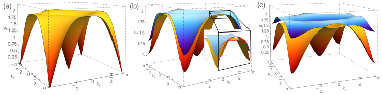
Figure 2: Spin-wave dispersion for (a) $v_{x}=w_{x}=v_{y}=w_{y}=0.0$, $J_{+}=1.0$, (b) $v_{x}=0.05$, $w_{x}=0.025$, $v_{y}=0.05$, $w_{y}=0.05$, $J_{+}=0.8$, (c) $v_{x}=0.2$, $w_{x}=0.05$, $v_{y}=0.2$, $w_{y}=0.2$, $J_{+}=0.8$. The inset of (b) highlights a pair of degenerate points that emerge with the introduction of anisotropic couplings. Another pair of degenerate points along the $k_{x}$-axis is not visible in the figure.

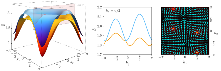
Figure 3: (left) Spin-wave dispersion for $v_{x}=0.1$, $w_{x}=0.05$, $v_{y}=0.1,w_{y}=-0.1$, $J_{+}=0.8$. (center) Cut along $k_{x}=\pi/2$ (indicated by red region in left panel). (right) Berry connection vector. The direction is indicated by the arrows while the color plot shows the magnitude.

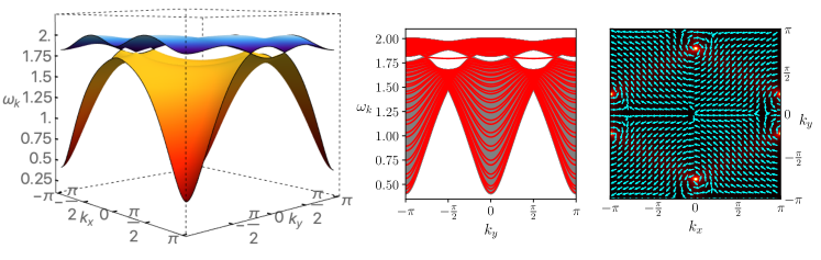
Figure 4: (left) Spin-wave dispersion for $v_{x}=0.364$, $w_{x}=0.0455$, $v_{y}=0.273,w_{y}=0.273$, $J_{+}=0.723$. (center) Edge spectrum, bulk shown in gray. (right) Berry connection vector. The direction is indicated by the arrows while the color plot shows the magnitude.

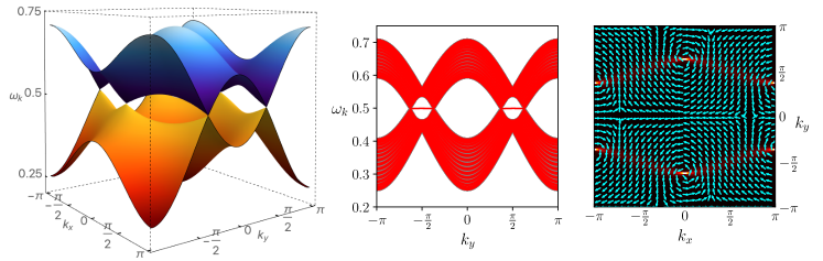
Figure 5: (left) Spin-wave dispersion for $v_{x}=0.4$, $w_{x}=0.1$, $v_{y}=w_{y}=0.625$, $J_{+}=0.25$. (center) Edge spectrum, bulk shown in gray. (right) Berry connection vector. The direction is indicated by the arrows while the color plot shows the magnitude.

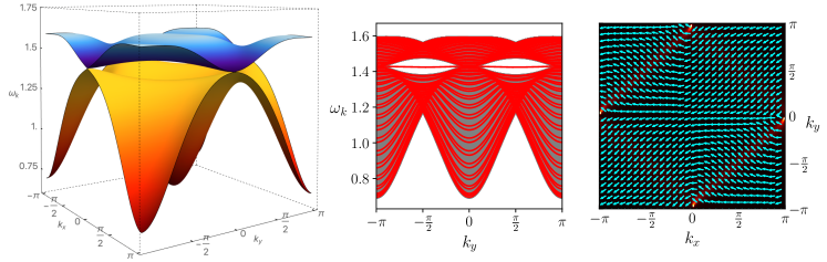
Figure 6: (left) Spin-wave dispersion for $v_{x}=0.357$, $w_{x}=0.143$, $v_{y}=0.286$, $w_{y}=0.214$, $J_{+}=0.571$. (center) Edge spectrum, bulk shown in gray. (right) Berry connection vector. The direction is indicated by the arrows while the color plot shows the magnitude.

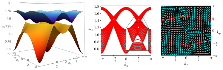
Figure 7: (left) Spin-wave dispersion for $v_{x}=0.214$, $w_{x}=0.071$, $v_{y}=0.571$, $w_{y}=0.5$, $J_{+}=0.571$. (center) Edge spectrum, bulk shown in gray. (right) Berry connection vector. The direction is indicated by the arrows while the color plot shows the magnitude.

In addition to the cases highlighted above (1-6 in Table 1), we note four additional special cases. First, if none of the cases 1-6 occur, then the coefficients $v_{x}\pm w_{x}\neq 0$ and $v_{y}\pm w_{y}\neq 0$, so we can rewrite Eqs. (18) as,

$$\cos(k_{x}a)= -\alpha\cos(k_{y}a),$$ (20)

$$\sin(k_{x}a)= -\beta\sin(k_{y}a),$$ (21)

where we have defined,

$$\beta\equiv \,{{v_{y}-w_{y}}\over{v_{x}-w_{x}}},$$ (23)

$$\alpha\equiv \,{{v_{y}+w_{y}}\over{v_{x}+w_{x}}}.$$ (24)

The solutions corresponding to the four combinations of $\alpha=\pm 1$, $\beta=\pm 1$, which represent lines of degeneracy, are given as cases 7-10 in Table 1.

When none of these ten special cases occurs, i.e, when $|v_{y}|\neq|w_{y}|$ and $|v_{x}|\neq|w_{x}|$, and $\alpha\neq 1$ (and $\beta\neq 1$), the general solution to the system of Eqs. (18), (19) gives the momenta at which Weyl-points occur:

$$k_{x}a =\cos^{-1}[\mp\alpha\Lambda]$$ (25)

$$k_{y}a =\cos^{-1}[\pm\Lambda],$$ (26)

where $\Lambda\equiv\sqrt{(\beta^{2}-1)/(\beta^{2}-\alpha^{2})}$.

Having classified the various phases exhibiting topological features, including Weyl points and lines of degeneracy, we proceed by presenting examples of the band structure, edge spectrum, and Berry connection (defined as $\mathbf{A}=-i\langle\psi_{0}|\boldsymbol{\nabla}_{\mathbf{k}}|\psi_{0}\rangle$, where $|\psi_{0}\rangle$ is the ground state), for these different states.

III.1 Solutions with Weyl-points

We begin by considering cases 1, 2, 4, and 5 of Table 1, as well as the general case given by Eqs. (25), (26), all of which yield spin-wave spectra with Weyl points.

We first present the case of isotropic coupling ($J_{+}=J_{z}=1.0$, with all other parameters equal to zero), which corresponds to the well-known nearest-neighbor antiferromagnetic Heisenberg model on the square-lattice, in order to provide a comparison for the spin-wave dispersions for the cases with anisotropic couplings. Fig. 2(a) shows the spin-wave dispersion for the isotropic case, which displays the well-known linear momentum dependence near $\mathbf{k}=0$ and at $\mathbf{k}=(\pm\pi/a,\pm\pi/a)$. In this case, the bands associated with $\omega^{+}$ and $\omega^{-}$ are degenerate. The introduction of coupling terms between the two sublattices ($v_{\alpha},w_{\alpha}$) breaks this degeneracy. If $J_{+}<J_{z}$ a gap opens at $\Gamma$ (and $(\pm\pi/a,\pm\pi/a)$), which can lead to non-trivial topological band structures.

Figs. 2(b)-(c) illustrate the presence of pairs of Weyl-point solutions, given by case 1 of Table 1, for small values of $v_{x},v_{y},w_{x},w_{y}$, i.e., for small deviations from the isotropic limit. Note that case 2 is equivalent to case 1 with the $x$ and $y$ axes interchanged. Both of these cases represent situations where the inversion symmetry is broken in either the $x$ or $y$ direction.

Fig. 3 shows an example of case 4. Notice that there are two pairs of Weyl points at the location given in Table 1, which are seen as singularities of the Berry-connection vector shown in Fig 3(c). Case 5 is obtained from case 4 by interchanging the $x$ and $y$ axes.

We continue by exploring several different parameter sets, with larger deviations from the isotropic limit, that display unique topological features. Fig. 4 and Fig. 5 give the calculated spin-wave dispersion (left), edge spectrum superimposed on the bulk states, which are projected as a gray background ribbon (center), and the Berry connection vector (right). To compute the edge spectrum we treat a system with semi-open boundary conditions that has $N_{x}=50$ layers along the $x$-direction and is periodic along the $y$-direction. In both cases, there are edge states that connect the bulk Weyl points in the lower (upper) half of the Brillouin zone at $k_{x}=0$ to those in the lower (upper) half of the Brillouin zone at $k_{x}=\pi$. The right panel demonstrates that there is a $2\pi$ counter-clockwise and a $2\pi$ clockwise rotation of the Berry connection vector as we travel around the positive and negative pseudo-helicity Weyl point, respectively.

Fig. 6 again shows the calculated spin-wave dispersion, the edge spectrum superimposed on the bulk states, and the Berry connection vector (using the same notations as in Fig. 4) for a special case of parameters which gives $\alpha=1$ but $\beta\neq\pm 1$, meaning degenerate points exist at $k_{x}=0$, $k_{y}a=\pm\pi$ and vice versa. In this case, we find a quadratic dispersion at the gapless band touching point. In this parameter regime, when $\alpha>1$ there are two pairs of Weyl points that merge at $k_{x}=0$, $k_{y}a=\pm\pi$ and $k_{x}a=\pm\pi$, $k_{y}=0$ as $\alpha\rightarrow 1$, yielding the quadratic band touching point we observe. For $\alpha<1$ there is no solution to Eqs. (20),(21), so the system is gapped.

Fig. 7 illustrates a situation where the anisotropy is large and as a result the edge-state has significant dispersion along the $\mathbf{k}$ direction parallel to the edge (in this case $k_{y}$). This case is similar to that shown in Fig. 5, however here $v_{y}\neq w_{y}$, which causes the Weyl points to shift away from $k_{x}=\pm\pi$ and $k_{x}=0$, and leads to a dispersive edge-state.

III.2 Solutions with lines of degeneracy

In this subsection we consider parameter sets that lead to solutions with lines of degeneracy; these correspond to cases 3, and 6-10 of Table 1.

Fig. 8(a) illustrates case 3 of Table 1, while Fig. 8(c) presents an example of case 7, where $\alpha=1$ and $\beta=1$, in which case, there is a pair of lines of degeneracy at $k_{y}=\pm\pi+k_{x}$. Figs. 8(b),(d) show the spin-wave dispersions along the path in the Brillouin zone indicated in the inset of Fig. 8(b), which crosses the lines of degeneracy in several locations.

Finally, we consider cases 10 and 6 of Table 1, which also correspond to lines of degeneracy. Fig. 9(a) is an example of case 10 where $\alpha=\beta=-1$, which results in a line of degeneracy at $k_{y}=k_{x}$. Fig. 9(c) is an example of case 6 where the couplings $v_{x}$ and $v_{y}$ in the $+x$ and $+y$ directions respectively are opposite to those in the $-x$ and $-y$ directions. Note that in both of these cases the global degeneracy present in the isotropic limit is broken. Moreover, the spin-wave dispersions are linear near $\mathbf{k}=0$ and $\mathbf{k}=(\pm\pi/a,\pm\pi/a)$, suggesting a pair of spin waves with different velocities along the longitudinal and transverse directions. This behavior is evident in Figs. 9(b),(d), which show the spin-wave dispersions along the path in the Brillouin zone indicated in the inset of Fig. 9(b).

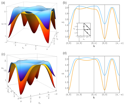
Figure 8: (a) Spin-wave dispersion for $v_{x}=0.1$, $w_{x}=0.1$, $v_{y}=0.05$, $w_{y}=0.05$, $J_{+}=0.8$. (b) Path through Brillouin zone (as shown in inset) for parameters in (a). (c) Spin-wave dispersion for $v_{x}=0.1$, $w_{x}=0.05$, $v_{y}=0.1$, $w_{y}=0.05$, $J_{+}=0.8$. (d) Path through Brillouin zone for parameters in (c).

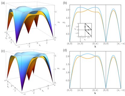
Figure 9: (a) Spin-wave dispersion for $v_{x}=0.1$, $w_{x}=0.05$, $v_{y}=-0.1$, $w_{y}=-0.05$, $J_{+}=1.0$. (b) Path through Brillouin zone (as shown in inset) for parameters in (a). (c) Spin-wave dispersion for $v_{x}=0.1$, $w_{x}=-0.1$, $v_{y}=0.05$, $w_{y}=-0.05$, $J_{+}=1.0$. (d) Path through Brillouin zone for parameters in (c)

IV Conclusion

In the present work, we have considered a slight modification of the familiar isotropic Heisenberg antiferromagnet on a square lattice, a model that is believed to describe a variety of non-geometrically frustrated spin systems, either as is, or as the foundation of Hamiltonians that describe a vast set of magnetic systems.

We have discovered that by allowing the $J_{x}$ and $J_{y}$ coupling constants to differ from $J_{z}$, so that their values become slightly different for different orientations of the nearest-neighbor bonds, thereby breaking the inversion symmetry of the lattice, the model can host interesting magnetic excitations with fascinating topological character.

We are able to analytically solve the modified model, within the spin-wave approximation, i.e., by taking into account the role of quantum-spin fluctuations around a Néel ordered state. The magnetic Bravais-lattice unit-cell remains the same as in the simpler case of the antiferromagnetic order, however, because our model breaks inversion symmetry, the degeneracy of the magnon dispersion is lifted and we obtain a pair of magnon dispersions which can cross at lines of degeneracy, or form singular pairs of Weyl points with opposite topological charge associated with a pseudo-helicity. In order to characterize the topological nature of these singularities, we have calculated the edge spectrum and the field of the Berry connection vector. We find that the model can host pairs of Weyl-magnon states with opposite topological charge connected by Weyl-arc edge states. In addition, we find parameter regimes characterized by lines of degeneracy.

Given that the nearest-neighbor Heisenberg antiferromagnet finds ubiquitous application in various magnetic materials, our findings may be easily realizable in nature. In fact, the slight modifications between the $x$-$y$ and $z$ components of the Hamiltonian discussed in this work are expected to be necessary to describe the magnetic excitations of a wide variety of two-dimensional antiferromagnets. In general, such anisotropic couplings should be expected when the antiferromagnet undergoes structural transition at lower temperature to phases of lower symmetry, such as orthorhombic or monoclinic structures. In a similar fashion, Peierls distortion can lead to different values for the $J_{-}$ coupling in the forward and backward bonds along a given direction, due to differences in bond length caused by the distortion. The parent compounds of the cuprate superconductors, for example La₂CuO₄, undergo a tetragonal to orthorhombic transition at lower temperature. In the orthorhombic phase, the structural distortions of the 2D Cu-O lattice should modify the couplings in such a way that this or other parent compounds of the family of oxides could host some of the states found in the present work.

In addition, continual progress in the field of ultra-cold atoms suggests that our model could be artificially engineered in optical lattices, where the conventional version of such a model has already been simulated [23, 24].

References

- Anderson [1987] P. W. Anderson, The Resonating Valence Bond State in La2CuO4 and Superconductivity, Science 235, 1196 (1987).
- Manousakis [1991] E. Manousakis, The spin-½ Heisenberg antiferromagnet on a square lattice and its application to the cuprous oxides, Rev. Mod. Phys. 63, 1 (1991).
- Anderson [1973] P. Anderson, Resonating valence bonds: A new kind of insulator?, Materials Research Bulletin 8, 153 (1973).
- Hasan and Kane [2010] M. Z. Hasan and C. L. Kane, Colloquium: Topological insulators, Rev. Mod. Phys. 82, 3045 (2010).
- Bernevig et al. [2006] B. A. Bernevig, T. L. Hughes, and S.-C. Zhang, Quantum Spin Hall Effect and Topological Phase Transition in HgTe Quantum Wells, Science 314, 1757 (2006).
- Fu et al. [2007] L. Fu, C. L. Kane, and E. J. Mele, Topological Insulators in Three Dimensions, Phys. Rev. Lett. 98, 106803 (2007).
- Bernevig and Hughes [2013] B. A. Bernevig and T. L. Hughes, Topological insulators and topological superconductors (Princeton University Press, Princeton, 2013).
- Armitage et al. [2018] N. P. Armitage, E. J. Mele, and A. Vishwanath, Weyl and Dirac semimetals in three-dimensional solids, Rev. Mod. Phys. 90, 015001 (2018).
- Wan et al. [2011] X. Wan, A. M. Turner, A. Vishwanath, and S. Y. Savrasov, Topological semimetal and Fermi-arc surface states in the electronic structure of pyrochlore iridates, Phys. Rev. B 83, 205101 (2011).
- Zhang et al. [2021] H. Zhang, C. Xu, C. Carnahan, M. Sretenovic, N. Suri, D. Xiao, and X. Ke, Anomalous Thermal Hall Effect in an Insulating van der Waals Magnet, Phys. Rev. Lett. 127, 247202 (2021).
- Li et al. [2016] F.-Y. Li, Y.-D. Li, Y. B. Kim, L. Balents, Y. Yu, and G. Chen, Weyl magnons in breathing pyrochlore antiferromagnets, Nature Communications 7, 12691 (2016).
- Jian and Nie [2018] S.-K. Jian and W. Nie, Weyl magnons in pyrochlore antiferromagnets with an all-in-all-out order, Phys. Rev. B 97, 115162 (2018).
- Li and Nevidomskyy [2021] S. Li and A. H. Nevidomskyy, Topological Weyl magnons and thermal Hall effect in layered honeycomb ferromagnets, Phys. Rev. B 104, 104419 (2021).
- Chen et al. [2018] L. Chen, J.-H. Chung, B. Gao, T. Chen, M. B. Stone, A. I. Kolesnikov, Q. Huang, and P. Dai, Topological Spin Excitations in Honeycomb Ferromagnet , Phys. Rev. X 8, 041028 (2018).
- Zhang and Yao [2023] M.-H. Zhang and D.-X. Yao, Topological magnons on the triangular kagome lattice, Phys. Rev. B 107, 024408 (2023).
- Liu et al. [2023] J. Liu, L. Wang, and K. Shen, Tunable topological magnon phases in layered ferrimagnets, Phys. Rev. B 107, 174404 (2023).
- McClarty [2022] P. A. McClarty, Topological Magnons: A Review, Annual Review of Condensed Matter Physics 13, 171 (2022).
- Joshi [2018] D. G. Joshi, Topological excitations in the ferromagnetic Kitaev-Heisenberg model, Phys. Rev. B 98, 060405 (2018).
- Xu et al. [2020] Q.-R. Xu, V. P. Flynn, A. Alase, E. Cobanera, L. Viola, and G. Ortiz, Squaring the fermion: The threefold way and the fate of zero modes, Phys. Rev. B 102, 125127 (2020).
- Rosenberg and Manousakis [2022] P. Rosenberg and E. Manousakis, Topological superconductivity in a two-dimensional Weyl SSH model, Phys. Rev. B 106, 054511 (2022).
- Rosenberg and Manousakis [2021] P. Rosenberg and E. Manousakis, Weyl nodal-ring semimetallic behavior and topological superconductivity in crystalline forms of Su-Schrieffer-Heeger chains, Phys. Rev. B 104, 134511 (2021).
- Colpa [1978] J. Colpa, Diagonalization of the quadratic boson hamiltonian, Physica A: Statistical Mechanics and its Applications 93, 327 (1978).
- Simon et al. [2011] J. Simon, W. S. Bakr, R. Ma, M. E. Tai, P. M. Preiss, and M. Greiner, Quantum simulation of antiferromagnetic spin chains in an optical lattice, Nature 472, 307 (2011).
- Brown et al. [2017] P. T. Brown, D. Mitra, E. Guardado-Sanchez, P. Schauß, S. S. Kondov, E. Khatami, T. Paiva, N. Trivedi, D. A. Huse, and W. S. Bakr, Spin-imbalance in a 2D Fermi-Hubbard system, Science 357, 1385 (2017).