100-fold improvement in relaxed eddy accumulation flux estimates through error diffusion

Abstract

Measurements of atmosphere-surface exchange are largely limited by the availability of fast-response gas analyzers; this limitation hampers our understanding of the role of terrestrial ecosystems in atmospheric chemistry and global change. Current micrometeorological methods, compatible with slow-response gas analyzers, are difficult to implement or rely on empirical parameters that introduce large systematic errors.

Here, we develop a new micrometeorological method, optimized for slow-response gas analyzers, that directly measures exchange rates of different atmospheric constituents with minimal requirements. The new method requires only sampling air at a constant rate and directing it into one of two reservoirs, depending on the direction of the vertical wind velocity. An integral component of this technique is an error diffusion algorithm that minimizes the biases in the measured fluxes and achieves direct flux estimates.

We demonstrate that the new method achieves accuracy within 0.1% of state-of-the-art eddy covariance measurements and its utility in maximizing the signal-to-noise ratios of measured scalars. Our new method provides a simple and reliable way to address complex environmental questions and offers a promising avenue for advancing our understanding of ecological systems and atmospheric chemistry.

Keywords Micrometeorology  $\cdot$ Flux measurements  $\cdot$ Eddy covariance  $\cdot$ Relaxed eddy accumulation  $\cdot$ Conditional sampling

1 Introduction

Surface exchange rates, or fluxes, of different atmospheric constituents are key metrics for investigating and understanding the interactions between the atmosphere and the biosphere (Baldocchi, 2020). The uncertainty over the distribution of atmospheric species emissions and losses at Earth’s surface poses a major limitation to our understanding of atmospheric chemistry and the role of the terrestrial surface in global climate (Arneth et al., 2010). Flux studies provide valuable insights into the cycling of trace elements like $\mathrm{CO_{2}}$, monitor the emission and disposition of pollutants for public health and air quality research, and contribute to better representation of different atmospheric constituents in climate models (Scholes et al., 2003; Fowler et al., 2009).

Micrometeorological methods are employed to measure atmospheric exchange in the lower atmosphere near the surface, where transport is predominantly turbulent, causing gases to diffuse rapidly to and from the surface. The flux is determined as the average product of the vertical wind velocity ($w$) and the scalar density ($c$). The direct calculation of this flux, achieved by assessing the covariance of $w$ and $c$ using the eddy covariance method, is widely recognized as the most direct and reliable way for measuring atmospheric fluxes at the scale of plant canopies (Dabberdt et al., 1993; Hicks and Baldocchi, 2020).

Atmospheric exchanges occur over various spatial and temporal scales, requiring high-frequency measurements (above 10 Hz) of wind velocity and scalar concentration to capture all flux-carrying motions. This high sampling requirement has limited the eddy covariance method to few atmospheric constituents, like water vapor and carbon dioxide, which have fast-response gas analyzers. Yet, many constituents critical to atmospheric chemistry and ecosystem dynamics, such as stable isotopes, nitrogen oxides, and volatile organic compounds, only have slow-response analyzers. For these, several alternative micrometeorological methods compatible with slower analyzers have been developed (Rinne et al., 2021). The true eddy accumulation (TEA) method realizes the product between $w$ and $c$ by accumulating air samples with mass proportional to the vertical wind velocity, enabling the direct measurement of the flux from the accumulated mass difference (Desjardins, 1977; Hicks and McMillen, 1984). However, the precise and fast control of air mass flow rate at the necessary dynamic range required for TEA implementation presents a significant challenge. This has limited te number of successful implementations of the TEA method and has prevented its widespread adoption (Siebicke and Emad, 2019). A simplification of the eddy accumulation method was proposed by (Businger and Oncley, 1990), which draws parallels to flux gradient methods by linking flux with the difference between updraft and downdraft concentrations. Unlike TEA, the relaxed eddy accumulation method (REA) does not require proportional mass flow control; instead, air samples are collected at a constant flow rate into updraft and downdraft reservoirs depending on vertical wind direction. The flux in REA is found as the product of the difference between accumulated scalar concentrations ($\Delta C$), wind standard deviation $(\sigma_{w})$, and an empirical coefficient $\beta$. The interpretation and determination of the empirical coefficient $\beta$ have remained the primary questions concerning the REA method (Baker, 2000; Katul et al., 2018; Vogl et al., 2021). While the theoretical value of $\beta$ derived assuming a Gaussian distribution for wind and scalar is $\beta\approx 0.63$ (Wyngaard and Moeng, 1992), observed average values of $\beta$ typically range between 0.47 and 0.63 and exhibit substantial run-to-run variability (Gao, 1995; Katul et al., 1996; Tsai et al., 2012; Grelle and Keck, 2021). These variations are attributed to diverse stability conditions, scalars, and site-specific factors (Sakabe et al., 2014; Ammann and Meixner, 2002). The absence of a reliable method for estimating or parametrizing $\beta$ has made it a major source of uncertainty in REA flux measurements, potentially introducing biases of up to 20% of the flux (Oncley et al., 1993; Gao, 1995).

Despite the high measurement uncertainty associated with $\beta$ variability, the REA method remains widely used for atmospheric exchange measurements due to its simple implementation requirements and its ability to increase scalar signal-to-noise ratios by excluding lower wind speeds using a deadband. REA has been applied to measure the fluxes of a wide array of atmospheric constituents. These include stable isotopes, hydrocarbons, methane, volatile organic compounds, ammonia, sulfate, nitrous oxide, mercury, aerosol numbers and dry deposition, halocarbon fluxes, peroxyacetyl nitrate, sodium chloride particle, and benthic solute fluxes in aquatic environments (Beverland et al., 1996; Haapanala et al., 2006; Bowling et al., 1999; Zhu et al., 1999; Pattey et al., 1999; Ciccioli et al., 2003; Matsuda et al., 2015; Hensen et al., 2009; Grelle and Keck, 2021; Skov et al., 2006; Meyers et al., 2006; Osterwalder et al., 2016; Held et al., 2008; GröNholm et al., 2007; Hornsby et al., 2009; Ren et al., 2011; Moravek et al., 2014; Meskhidze et al., 2018; Calabro-Souza et al., 2023; Riederer et al., 2014).

In this paper, we propose a new direct eddy accumulation method that combines the simple requirements of relaxed eddy accumulation with the accuracy and robustness of the conventional eddy covariance technique. The new method employs error diffusion to achieve reliable and direct flux estimates with minimal bias, typically less than 0.1% of the reference flux from eddy covariance, without the need for empirical estimation coefficients. We begin with a novel theoretical derivation for conditional sampling, where we formulate sample accumulation as a quantization problem and introduce an error diffusion algorithm to randomize the quantization error. This is followed by a detailed examination of the signal and noise shaping properties of error diffusion. We derive an expression for the error in our method and discuss how error diffusion effectively minimizes the quantization error. Finally, we test the performance of our method with numerical simulations. We explore the ideal parameters for quantization and discuss implementation details.

2 Theory

2.1 Derivation of quantized eddy accumulation

In the following, we derive the generalized equation for conditional sampling. We consider the flux of an atmospheric constituent $c$, such as $\mathrm{CO_{2}}$

$$F=\overline{wc}=\overline{w^{\prime}c^{\prime}}+\bar{w}\bar{c}$$ (1)

Here, $w$ represents the vertical wind velocity ($\mathrm{m}\,\mathrm{s}^{-1}$), and $c$ represents the molar density ($\mathrm{mol}\,\mathrm{m}^{-3}$) of the scalar in question. Overlines indicate averaging that follows Reynolds averaging rules, while the primes indicate deviations from the mean. The previous equation can be derived from conservation laws. For a detailed discussion of surface flux equations, refer to Finnigan et al. (2003) and Foken et al. (2012). The definition in Eq. 1 is chosen as eddy accumulation methods measure, by definition, the term $\overline{wc}$. The term $\bar{w}\bar{c}$ is typically biased due to inaccuracies in $w$ (Emad and Siebicke, 2023a). Depending on the used concentration index, the separation into turbulent and systematic transport, as well as estimating physical $\bar{w}$ still applies similar to EC measurements (Kowalski, 2017; Kowalski et al., 2021). However, these aspects do not change the subsequent analysis.

We apply a quantizer function $Q(w)$ to restrict the possible values of $w$ to a finite, discrete set. To ensure high flexibility and ease of implementation in flux measurements, we consider a non-uniform quantizer with three levels: $(-w_{f},\,0,\,+w_{f})$. These quantization levels do not need to be uniformly spaced. The quantizer function compares measured wind speeds with a quantization threshold, denoted as $q_{t}$. If the measured wind speed exceeds this threshold, the quantized value of $w$ becomes the full scale value $w_{f}$ or $-w_{f}$ depending on its direction. The quantizer function is expressed as

$$Q(w,~{}q_{t},~{}w_{f})=\begin{cases}\mathrm{sign}(w)\,w_{f},&\text{if}\,|w|>q_{t}\\ 0,&\text{if}\,|w|\leq q_{t}\end{cases}$$ (2)

We define the quantization error $\varepsilon_{q}$ as the difference between the true value of $w$ and the quantized output

$${\varepsilon}_{q}=w-w_{q}$$ (3)

Consequently, the flux can be written as the sum of the flux of the quantized wind signal and the flux of the quantization error

$$\overline{w\,c}=\overline{c(w_{q}+\varepsilon_{q})}=\overline{w_{q}\,c}+\overline{\varepsilon_{q}\,c}.$$ (4)

We can further express the flux of the quantized wind as the conditional expectation of the random variable $c\,w_{q}$, based on a variable $I$ that partitions the probability space into finite, non-overlapping partitions. This approach forms the foundation of our analysis.

$$F_{qea}=\overline{c\,w_{q}|I}+\overline{\varepsilon_{q}\,c}.$$ (5)

The previous equation shows that the flux estimate derived from a quantized wind signal is biased by the covariance between the quantization error and scalar concentration. This bias arises because the quantization error is not random but deterministic and correlated with both the original wind speed and the scalar concentration. To minimize this error, we propose a solution by reintroducing the quantization error into the signal through a feedback loop. This process is similar to introducing pseudorandom noise to the signal, a technique known as dithering by error diffusion (Knox, 1999). Similar approaches are commonly employed in image and audio processing applications to enhance the perceptual quality of quantized signals (Kite et al., 1997; Escbbach et al., 2003). In this approach, with each new wind measurement, we subtract the quantization error of the previous measurement from the new measurement before quantizing it.

$$w_{q}[n]=Q\left(w[n]-{\varepsilon_{q}}[n-1]\right)$$ (6)

2.2 Analysis of error diffusion

The first step of quantization and error diffusion is forming the modified input. This is achieved by subtracting "diffused" past error terms from the input. The diffusion is represented by the linear weighting filter, denoted as $h$, which includes only past errors and, as such, is causal

$$u(n)=x(n)-\sum_{k\in\mathcal{O}}h(k)e(n-k),$$ (7)

Here, $u(n)$ represents the modified input, $x(n)$ corresponds to the input of the system, and $\mathcal{O}$ is the causal support set that does not include 0, signifying that it only includes past errors.

In the second step, the output of the system $y(n)$ is calculated by applying the quantization function $Q(.)$ to the modified input.

$$y(n)=Q(u(n))$$ (8)

The quantizer error $e(n)$ is defined as the difference between the output, $y(n)$ , and the modified input

$$e(n)=y(n)-u(n),$$ (9)

we substitute Eq. 7 into Eq. 9, we find

$$e(n)=y(n)-x(n)+\sum_{k\in\mathcal{O}}h(k)e(n-k)$$ (10)

The previous equation highlights the recursive character of error diffusion, where the error at any given moment in time depends on the entire past history. We apply the $z$-transform to Eq. 10 and rearrange it as follows:

$$Y(z)-X(z)=(1-H(z))E(z)$$ (11)

Here, $H(z)=\sum h(k)z^{k}$, is the filter applied to past errors in the frequency domain. Considering that $G(z)=Y(z)-X(z)$ represents the total quantization error, which corresponds to the output of the noise transfer function, we find the transfer function describing the frequency shaping of the noise by rearranging the previous equation to be

$$\frac{G(z)}{E(z)}=1-H(z)$$ (12)

Equation 11 indicates that the total quantization error $(\varepsilon_{q})$, defined as the difference between the system output and its input, consists of two errors one of them is a filtered version of the other. The first error component is the quantizer error $E(z),$ which we defined as the difference between the output and the modified input. The second error component is the filtered quantizer error, which we call the diffusion error $E(z)H(z)$.

Error diffusion can be viewed as an error minimization process. It aims to reduce the difference between the input and the output by adjusting the weights of a linear filter (Escbbach et al., 2003). In our specific application, $H(z)$ is constrained to be causal, the unit delay filter, denoted as $H(z)=z^{-1}$, emerges as the optimal solution for minimizing the correlation of the quantization error with the scalar. This filter allows all frequencies to pass unattenuated and introduces a linear phase shift, which, in this case, results in a one-sample delay of the input. The previous equation with H(z) as the unit delay filter indicates that the mean of the output is equal to the mean of the input. This equality is due to the filter coefficients summing to one, therefore at dc, $H(1)=1$. As our primary interest lies not in the quantization error itself, but rather in its correlation with the scalar concentration $c$, we can write the quantization error covariance term as

$$\overline{\varepsilon_{q}^{\prime}\,c^{\prime}}=\overline{e^{\prime}c^{\prime}}-\overline{(h*e)^{\prime}c^{\prime}},$$ (13)

where $*$ indicates convolution. Given that the diffusion error represents a one-sample delayed version of $e(n)$ and based on the definition of the cross-covariance function between $e$ and $c$, denoted as $R_{ec}(n)$, we can express the error covariance as:

$$\overline{\varepsilon_{q}^{\prime}\,c^{\prime}}=R_{ec}(0)-R_{ec}(1)$$ (14)

In general, $e$ is typically assumed to be white noise for a uniform quantizer. However since $e$ is formed deterministically from $w$, it exhibits a weak correlation with $w$ in particular if the quantizer is non-uniform. Modeling the quantizer directly can be challenging due to its nonlinearity. Nevertheless, it was shown that the quantizer can be approximated by a linear gain (Kite et al., 2000). Therefore, we can establish a linear relationship between the cross-covariance functions $R_{ec}$ and $R_{cw},$ expressed as $R_{ec}=KR_{wc},$ with $K$ being an empirical coefficient determined through a least square approach. We further assume that the covariance function $R_{wc}$ is exponential such that $R_{ec}(\tau)=\exp{(-\tau/T_{i})}$ where $T_{i}$ is the integral time scale. This allows us to derive the expression for the relative error in the flux as shown in Eq. 17.

It is important to note that the analysis presented constitutes a simplified approximation for a general understanding of error behavior. While the exponential covariance assumption may not always precisely hold, it remains a close approximation in practice. This is attributed to the consistent autocorrelation of $e$, with our primary focus being its behavior concerning a single delayed sample.

2.3 Simulation data and parameters

We used a high-frequency dataset of eddy covariance (EC) measurements, collected from an ideal flat agricultural field at the Thünen Institute in Braunschweig, Germany (52.30° N, 10.45° E), as the primary input for our simulation. For a detailed site description and instrumentation, please refer to (Emad and Siebicke, 2023b). The high-frequency dataset covered 12 days, from July 11, 2020, to July 25, 2020, with 606 30-minute averaging intervals. We used 3D wind velocity data measured by a sonic anemometer (uSonic-3 Class A, Metek GmbH, Germany) and gas concentration measurements for $\mathrm{CO_{2}}$ and $\mathrm{H_{2}O}$ using an open-path infra-red gas analyzer (LI-7500A, LI-COR Biosciences GmbH, Germany).

Using this dataset, we simulated flux measurements for three variables: $\mathrm{CO_{2}}$, $\mathrm{H_{2}O}$, and air temperature (Ts). Our simulation included the newly developed quantized eddy accumulation method and three relaxed eddy accumulation method variants, serving as baselines for performance benchmarking under the same constraints. The simulation aimed to assess the performance of the quantized eddy accumulation method with error diffusion and determine its optimal parameters for various objectives. The performance evaluation had two primary aims: first, to separate errors into systematic and random components, and second, to evaluate the quality of these errors, specifically checking for any correlations with flux values, time of day, or atmospheric stability.

To establish a performance baseline for the REA method, we calculated the average of the current state-of-the-art conditional sampling methods under the constrain of a constant air flow rate. Since there were no clear recommendations for calculating $\beta$ under different scalar and atmospheric conditions, we followed three recommended REA treatments from the literature to estimate the value of $\beta$ (Vogl et al., 2021). These treatments included a constant $\beta$ estimated as the median of $\beta$ calculated from air temperature ($\beta_{ts-median}$), as well as $\beta$ calculated from vertical wind velocity statistics using two dynamic deadband settings, namely, $0.5\sigma_{w}$ and $0.9\sigma_{w}$ (Baker, 2000). The baseline performance of REA was determined by averaging these three variants. Quantized eddy accumulation with error diffusion was simulated with a wide range of parameters. For performance comparison with REA variants, we specifically selected the parameter pair ($q_{t}=2,q_{\text{full}}=4$)

3 Results and Discussion

3.1 Quantized eddy accumulation with error diffusion

We found that relaxed eddy accumulation is equivalent to measuring the flux using a 1-bit quantized wind velocity within each wind direction. The emergence of $\beta$ is a result of the unaccounted flux portion transported by quantization errors. To minimize quantization errors, we developed an error diffusion algorithm that randomizes these errors, effectively reducing the flux biases to zero. As a result, we achieve highly accurate flux estimates without the need for the empirical coefficient $\beta$.

We have developed a novel approach that integrates various conditional sampling methods, such as relaxed eddy accumulation and its variants, into a single framework. The flux $\overline{cw}$ is expressed in this framework as:

$$\overline{cw}=\overline{c~{}Q(w)|I}=\overline{c\,w_{q}|I}+\overline{c\,\varepsilon_{q}},$$ (15)

where $w$ represents the vertical wind velocity, and $c$ denotes the concentration of a scalar of interest. The key insight of this framework is the quantization of wind velocity, which enables discretization of continuous wind velocities into a limited number of levels. A result of quantization, $w$ is decomposed into the quantized wind speed ($w_{q}$) and the quantization error ($\varepsilon_{q}$). The term $\overline{cw_{q}|I}$ denotes the conditional expectation of $cw_{q}$ with the partitioning variable $I$, and $\overline{c\varepsilon_{q}}$ accounts for the correlation between the quantization error and scalar concentration. Therefore, Eq. (15) indicates that the total flux $\overline{cw}$ is composed of two components: the flux associated with quantized wind speed ($\overline{cw_{q}|I}$) and the flux attributable to the quantization error ($\overline{c\epsilon_{q}}$).

In this framework, the conventional REA method arises when setting the conditioning variable $I$ to $\mathrm{sign}(w)$ and quantizing wind speed into two discrete levels that correspond to the means of updraft and downdraft wind: $\overline{w^{\uparrow}}$ and $\overline{w^{\downarrow}}$. Our framework reveals that $\beta$ is fundamentally linked to the flux carried with quantization errors arising from non-optimal quantization. This connection provides an explanation for the difficulty in estimating $\beta$ as it involves a part of the joint probability distribution that extends beyond the quantization boundaries and remains unobserved in our measurements. This framework not only aids in interpreting $\beta$ but also suggests that error reduction can be achieved through improvements in the quantization process, such as refining quantization boundaries and values.

While previous efforts mainly focused on improving $\beta$ estimates, framing this issue as a measurement of a quantized signal provides an innovative alternative. It allows us to exploit the noise shaping properties of error diffusion to enhance the representativeness of the quantized signal and reduce the correlation of the error with the scalar. Building upon this understanding, we have developed an error diffusion algorithm that effectively eliminates the correlation between the quantization error and the scalar, driving its expected value close to zero. The application of error diffusion to quantized wind signals has substantially reduced flux errors, rendering empirical $\beta$ unnecessary. We refer to this variant of eddy accumulation as quantized eddy accumulation (QEA) with error diffusion.

Algorithm 1 Quantized Eddy Accumulation With Error Diffusion

0:  vertical wind speed array $w$, quantization threshold $q\_threshold$, and wind quantized full scale value $w\_full$

1:  $N\leftarrow\text{length}(w)$

2:  $residual\_error\_up\leftarrow 0$

3:  $residual\_error\_down\leftarrow 0$

4:  for $i=1$ to $N$ do

5:     if $w[i]>0$ then

6:        $w_{mod}\leftarrow w-residual\_error\_up$

7:        $w_{q}[i]\leftarrow Q(w_{mod},~{}q\_threshold,~{}w\_full)$

8:        $residual\_error\_up\leftarrow w_{q}[i]-w_{mod}$

9:     else

10:        $w_{mod}\leftarrow w-residual\_error\_down$

11:        $w_{q}[i]\leftarrow Q(w_{mod},~{}q\_threshold,~{}w\_full)$

12:        $residual\_error\_down\leftarrow w_{q}[i]-w_{mod}$

13:     end if

14:  end for

15:  return  $w_{q}$

Our error diffusion algorithm, described in Algorithm 1, requires only a constant airflow rate for air sampling and the channelling of this airflow into either updraft or downdraft reservoirs depending on the sign of quantized wind. The quantization error in this algorithm is incorporated in a feedback loop with the measured vertical wind velocity before quantizing it into three discrete levels corresponding to updraft, downdraft, and no sampling. The error diffusion algorithm is seen as an error minimization mechanism, as pseudorandom noise is introduced into the signal to reduce the error correlation with the scalar.

The quantization of wind, similar to employing a deadband in REA, serves the purpose of filtering out low wind speed that are associated with weak scalar concentration. Increasing the quantization threshold enhances the difference in accumulated concentrations between updraft and downdraft reservoirs, thereby improving the signal-to-noise ratio. This concentration enhancement is especially useful when measuring atmospheric constituents with low flux. Importantly, this concentration enhancement does not introduce additional uncertainty due to error diffusion.

In summary, our new method provides a simple and reliable way to directly measure atmospheric exchange. It stands as the only method capable of increasing the signal-to-noise ratio without compromising measurement accuracy. The error diffusion algorithm eliminates the need for the empirical coefficient $\beta$, aligning our method with eddy covariance and true eddy accumulation.

3.2 Analysis of Error Diffusion

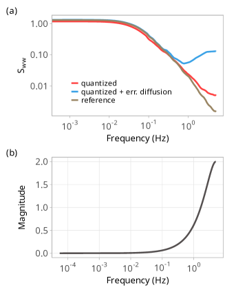
Figure 1: Spectral Analysis of Error Diffusion. (a) Normalized power spectral density of vertical wind velocity over a 30-minute period at midday in summer. The ’reference’ curve represents the original spectrum, while the ’quantized’ and ’quantized + error diffusion’ curves illustrate the effects of quantization and subsequent error diffusion on the signal. The noise shaping behavior is evidenced by the deviation of the ’quantized’ and ’quantized + error diffusion’ curves from the ’reference’, particularly in the higher frequency range. (b) Magnitude response of the noise transfer function, displaying the high-pass characteristics of the $G(z)=1-{z^{-1}}$ filter, with a steady increase in magnitude with frequency, demonstrating the noise shaping effect on the spectral content of the processed signal.

The analysis of error diffusion reveals that the quantizer noise is pushed towards the higher end of the spectrum, as shown in Figure 1. Consequently, the spectrum of the quantization error exhibits characteristics resembling blue noise, with a significant concentration of power in the high-frequency range. Examining the system response in the $z$-domain, we find that the noise transfer function of error diffusion can be expressed as:

$$NTF(z)=1-H(z),$$ (16)

where $H(z)$ represents a linear filter that is applied to past errors and which we considered as the unit delay filter ($1/z$) for our application. The noise transfer function $NTF(z)=1-{z^{-1}}$ exhibits a frequency response that amplifies higher frequencies, as indicated by the magnitude plot in Fig. 1. The gain increases linearly with frequency, peaking at twice the input signal’s amplitude at the Nyquist frequency. This characteristic introduces additional energy into the system at higher frequencies, effectively shaping the noise spectrum by attenuating lower frequencies while amplifying higher ones, which is beneficial in flux measurements as the noise at higher frequencies is typically more tolerable.

The analysis of the system has demonstrated that error diffusion is mean preserving; the mean output signal equals the mean of the input as the filter coefficients sum to unity. Furthermore, our analysis of error diffusion indicates that the total quantization error comprises two components, one of which is a filtered version of the other. We investigated the correlation of the quantization error with the scalar concentration by assuming a linear gain model of the quantizer and an exponential covariance function. This led us to derive an expression for the relative error in the flux:

$$\frac{\overline{\varepsilon_{q}^{\prime}\,c^{\prime}}}{\overline{c^{\prime}\,w^{\prime}}}=K(1-\exp(-\frac{1}{f_{s}\,T_{i}})),$$ (17)

where $T_{i}$ is the integral time scale, $f_{s}$ is the sampling frequency, and $K$ is an empirical coefficient that relates the error to the original signal. Values of $K$ were found to be generally below $0.1$, therefore for a typical range of $T_{i}$ values between $5$ to $10$ seconds and a sampling frequency of 10 Hz, we find the error described above to remain below $0.2\%$ of the flux.

3.3 Performance evaluation of error diffusion

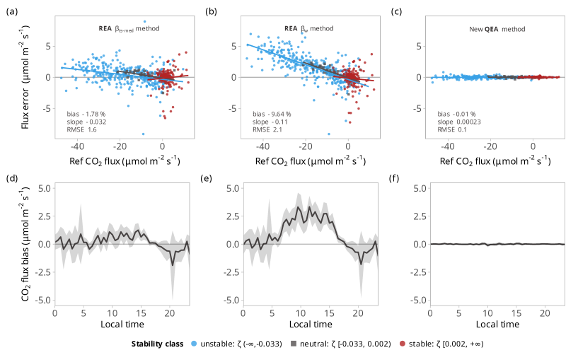
Figure 2: Performance Evaluation of Quantized Eddy Accumulation. (a)-(c) Scatter plots displaying the comparison between two established relaxed eddy accumulation (REA) methodologies ($\beta_{\text{ts-med}}$ and $\beta_{w}$) versus the novel quantized eddy accumulation (QEA) method with error diffusion. Flux errors for $\mathrm{CO_{2}}$ are presented as the discrepancy relative to eddy covariance reference flux measurements, differentiated by atmospheric stability classes: unstable (blue), neutral (red), and stable (beige). These categories illustrate the error’s sensitivity to atmospheric stability. Each method’s performance is quantified through bias (mean error), slope, and root mean square error (RMSE) statistics. (d)-(f) Diurnal profiles of $\mathrm{CO_{2}}$ flux biases for each method, with a 95% confidence interval shaded region generated via bootstrapping. This demonstrates the temporal variability of biases throughout the day, and underscores the QEA method’s robustness, as evidenced by its consistent closeness to the reference data, signifying minimal systemic error.

Table 1: Comparative performance evaluation of quantized eddy accumulation (QEA) with error diffusion versus conventional relaxed eddy accumulation (REA) methods for CO₂, H₂O, and $\theta$ (air temperature) fluxes. Performance metrics include error slope (dimensionless), error intercept (units of flux), error relative mean (dimensionless), and Root Mean Square Error (RMSE, units of flux). The ’Average improvement ratio’ highlights the mean enhancement QEA provides over REA variants, calculated as the ratio of REA’s average metric across all scalars to the QEA’s corresponding metric, demonstrating significant error reduction by QEA.

Variable	Method	Error slope	Error intercept	Error relative mean	RMSE
$\mathrm{CO_{2}}$	QEA with error diffusion	$2.3\times 10^{-4}$	$3.5\times 10^{-3}$	$-1.3\times 10^{-4}$	0.1194
	REA $(\mathrm{db}~{}{0.5\sigma})$ $\beta_{\mathrm{ts-median}}$	-0.0321	-0.1369	-0.0178	1.5865
	REA $(\mathrm{db}~{}{0.5\sigma})$ $\beta_{w}$	-0.1096	-0.1258	-0.0964	2.3173
	REA $(\mathrm{db}~{}{0.9\sigma})$ $\beta_{w}$	0.0111	-0.1873	0.0307	1.4876
H2O	QEA with error diffusion	$-9.6\times 10^{-5}$	$1\times 10^{-4}$	$-7.3\times 10^{-6}$	0.0169
	REA $(\mathrm{db}~{}{0.5\sigma})$ $\beta_{\mathrm{ts-median}}$	-0.0383	-0.0011	-0.0392	0.1236
	REA $(\mathrm{db}~{}{0.5\sigma})$ $\beta_{w}$	-0.1172	0.0009	-0.1163	0.2315
	REA $(\mathrm{db}~{}{0.9\sigma})$ $\beta_{w}$	0.0207	-0.0086	0.0133	0.1012
$\theta$	QEA with error diffusion	$-9.4\times 10^{-5}$	$6.1\times 10^{-6}$	$4.3\times 10^{-5}$	0.0004
	REA $(\mathrm{db}~{}{0.5\sigma})$ $\beta_{w}$	-0.0731	0.0002	-0.0695	0.0074
	REA $(\mathrm{db}~{}{0.9\sigma})$ $\beta_{w}$	0.0097	0.0003	0.0162	0.0041
	Average improvement ratio	422	38	3291	13

Our assessment of the newly developed error diffusion algorithm indicates a substantial enhancement in accuracy over conventional relaxed eddy accumulation methods. A simulation-based analysis revealed that systematic biases of QEA with error diffusion —quantified as the slopes of the error against flux values—were consistently below 0.1% of the reference eddy covariance fluxes. These biases are significantly lower than the average 5% bias found with the commonly used REA techniques, as shown in Figure 2.

Additionally, the QEA method introduced minimal random errors. The root mean square error (RMSE) for carbon dioxide $\mathrm{CO_{2}}$ flux measurements was about 0.11 $\mathrm{\mu\,mol\,m^{-2}\,s^{-1}}$, and for water vapor, it was about 0.02 $\mathrm{m\,mol\,m^{-2}\,s^{-1}}$, both significantly lower than those from REA methods by an order of magnitude. Importantly, the accuracy of QEA was not influenced by the time of day or atmospheric stability, unlike the REA methods, as shown in Figure 2. These findings, along with several other error metrics, are summarized in Table 1, demonstrating that QEA outperforms REA across all examined conditions.

With its reduced error rates, QEA offers a performance comparable to eddy covariance method and serves as an important new tool for studying surface-atmosphere exchanges, especially for constituents with very small fluxes previously too challenging to measure.

3.4 Optimal quantization parameters

Figure 3: Evaluation of Parameter Space for Systematic Bias and Error Variability in $\mathrm{CO_{2}}$ Flux Measurements. Panel (a) displays a heatmap that illustrates the systematic bias, represented by the slope of the linear fit, as a function of the quantization threshold and full-scale value. The color intensity corresponds to the magnitude of the systematic bias, with distinct color gradations marking predefined slope values. A white dashed line at a full-scale value of 2.3 indicates the boundary where systematic bias exceeds 1%. Panel (b) presents a heatmap of the maximum relative Root Mean Square Error (RMSE) to Standard Deviation (SD) expressed as a percentage, which indicates error variability. These metrics are calculated based on simulations utilizing the entire dataset.

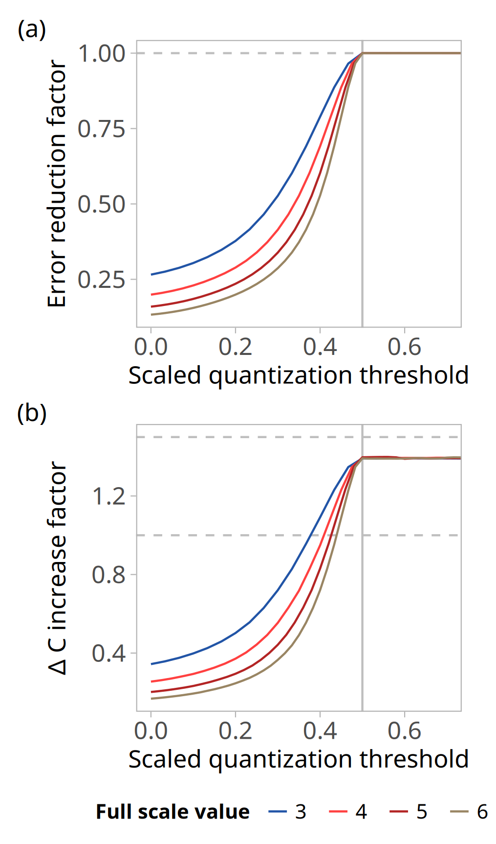
Figure 4: Error Reduction and $\Delta C$ Increase of Error Diffusion. (a) Error reduction factor against scaled quantization threshold, for full-scale values 3-6, illustrating the impact of quantization on mean vertical wind velocity error. (b) $\Delta C$ increase factor, representing the concentration difference between updraft and downdraft as ratio to $\Delta C$ with a quantization threshold of zero, plotted over the scaled quantization threshold. Horizontal lines at y=1 and y=1.5 serve as benchmarks. The scaled quantization threshold is the quantization threshold normalized to the full-scale value

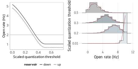
Figure 5: Valve Switching Dynamics. The left panel illustrates the relationship between the scaled quantization threshold and the average valve switching rate (Hz), distinguishing between reservoirs (’down’, solid line) and (’up’, dashed line). The right panel presents the distribution of valve switch events across different rates and for four distinct scaled quantization thresholds.

The developed error diffusion algorithm has two parameters: the quantization threshold ($q_{\text{threshold}}$) and the quantized full-scale value ($q_{\text{full}}$). The choice of these parameters allows for minimizing the flux error, maximizing the concentration difference in accumulation reservoirs ($\Delta C$), reducing the error due to nonzero mean vertical wind velocity, and controlling the switching rates of the sampling valves.

The main objective of the evaluation presented here was to establish optimal ranges for the quantizer parameters that optimize for the above goals. These goals were assessed through numerical simulations for three different scalars over a broad range of parameters. Simulation results indicated that, for all scalars, the flux error remained consistently low across a wide range of $q_{\text{threshold}}$ and $q_{\text{full}}$ combinations, as shown in Figure 3. Generally, the error stayed below 1% for almost any combination of parameters, provided that the full-scale value was greater than $2.4\sigma_{w}$. Notably, a large number of parameter combinations resulted in errors smaller than 0.1%. The variance of errors showed similar trends, with the Root Mean Square Error (RMSE) typically being lower for parameter combinations that minimized systematic errors.

Adjusting the quantization threshold can improve the Signal-to-Noise Ratio (SNR) by increasing the difference in concentration $\Delta C$ between the two accumulation reservoirs, as illustrated in Figure 4. The key factor is the ratio between the quantization threshold and the quantized full scale value, referred to as the scaled quantization threshold. Values greater than 0.5 can enhance $\Delta C$ by up to 150%, akin to introducing a deadband in REA measurements, which leads to the selective accumulation of eddies with concentrations far from the mean. However, unlike REA, selecting a quantization threshold at this level does not reduce the accuracy of flux measurements (Oncley et al., 1993; Pattey et al., 1993). Increasing the scaled quantization threshold has the opposite effect on errors related to non-zero mean vertical wind velocity. An increase in $\Delta C$ coincides with a decrease in wind variance (and thus, $\overline{|w|}$), which has been demonstrated to correlate with the magnitude of the flux error under conditions where the mean wind is not zero (Emad and Siebicke, 2023a). A scaled quantization threshold below 0.5 is effective in decreasing these wind-related errors as illustrated in Figure 4. A threshold set to zero can remove the influence of non-zero mean vertical wind velocity entirely, which is a unique advantage of QEA over TEA and REA.

Additionally, adjusting the scaled quantization threshold affects how often sampling valves switch and the accumulated sample volumes. Higher thresholds lead to less frequent switching; for example, with a threshold of 0.5, the updraft and downdraft valves switch on average once per second, as shown in Figure 5.

3.5 Implementation and flux calculation

The simplest form of quantized eddy accumulation with error diffusion is achieved using two reservoirs that accumulate air at a constant flow rate, similar to the requirements of the relaxed eddy accumulation method. We discuss the specifics of such an implementation here.

For this partitioning approach, the conditioning variable $I$ is the direction of vertical wind velocity, given by $I=\mathrm{sign}(w)$. However, this variable can also be used to facilitate further partitioning to carry sample accumulation on shorter time intervals which gives more implementation flexibility (Emad and Siebicke, 2023b). We consider the simple case of partitioning based on the sign of $w$, equation 15 becomes

$$F_{q}=\overline{w_{q}c}=\overline{c^{\uparrow}w_{q}^{\uparrow}}~{}p^{\uparrow}+\overline{c^{\downarrow}w_{q}^{\downarrow}}~{}p^{\downarrow}$$ (18)

The quantization of $w$ is achieved with three levels of quantization ($-w_{f}$, 0, and $w_{f}$), where $w_{f}$ is the quantized full scale level. This process is analogous to a 1-bit quantization of each updraft and downdraft wind speeds.

The choice of the quantization threshold ($q_{t}$) and the quantizer’s full scale setting ($w_{f}$) plays a crucial role in error control, signal-to-noise ratio (SNR) enhancement, and reduction of residual vertical wind velocity. Setting $q_{t}$ to zero allows for an unbiased estimation of $\bar{c}$, as it leads to $\overline{c^{\uparrow}w_{q}^{\uparrow}}=\overline{c^{\uparrow}}~{}\overline{w_{q}^{\downarrow}}$. This choice effectively eliminates errors associated with non-vanishing mean wind velocity, providing an advantage over traditional eddy accumulation methods.

Referring to Figure 3, we can identify the optimal quantization parameters $q_{t}$ and $w_{f}$. For instance, setting $q_{t}$ to $2.5\sigma_{w}$ and the full-scale value to $4\sigma_{w}$ predict an average error under $0.1\%$. Since these depend on the unknown $\sigma_{w}$ of the averaging interval, an estimate from the preceding interval can be used. The heatmap illustrates that the error diffusion is robust to slight variations in $\sigma_{w}$ which supports the use of past data to define the parameters of the current averaging interval. The chosen example parameters suggest nearly a 1.4-fold increase in $\Delta C$ and an average valve switching rate of about 2 Hz as seen from figures 4 and 5

In a typical implementation of this method, real-time vertical wind velocity is acquired and then adjusted through an online planar fit to align the coordinates to the streamline coordinates, as described in (Siebicke and Emad, 2019). We recommend subtracting the mean wind of the previous interval to minimize residual $\bar{w}$ and achieve a more symmetric distribution around zero. Subsequently, the wind speed is modified using the previous quantization error and then quantized. The process of quantization and error diffusion is detailed in Algorithm 1. If the quantized $w$ is non-zero, the flow is directed into the corresponding reservoir. The accumulated volume in each reservoir at the end of the averaging interval is calculated as $V=An_{q}T_{s}$, where $A$ represents a flow scaling factor and $T_{s}$ is the sampling interval. It is important to emphasize that the requirement for flow consistency applies only within each averaging interval and reservoir. Therefore, variations in flow are permissible between updraft and downdraft and across different averaging intervals. After the end of the averaging interval, typically spanning 30 minutes to 1 hour, the flux is computed based on the following equation

$$F_{\text{total}}=\overline{c^{\uparrow}}~{}\overline{w_{q}^{\uparrow}}\frac{n_{q}^{\uparrow}}{n}+\overline{c^{\downarrow}}~{}\overline{w_{q}^{\downarrow}}\frac{n_{q}^{\downarrow}}{n}-\bar{c}~{}\overline{w_{q}}+\overline{w_{q\epsilon}c},$$ (19)

where $\overline{c^{\uparrow}}$ and $\overline{c^{\downarrow}}$ represent the average scalar concentrations in updraft and downdraft reservoirs, while ${n_{q}^{\uparrow}}$ and ${n_{q}^{\downarrow}}$ indicate the counts of occurrences with the quantized wind direction as updraft and downdraft, respectively. The variable $n$ represents the total number of vertical wind velocity samples within the averaging interval. Since the measured quantities here are means rather than fluctuations, eddy accumulation methods are more robust to frequency losses due to the analyzer response and typically will not require spectral corrections (Emad, 2023).

Equation 19 involves the term $\bar{c}~{}\bar{w_{q}}$, which requires the knowledge of the scalar concentration within the averaging interval $\overline{c}$ to account for it. Estimating this term poses a common challenge in eddy accumulation methods and arises due to the presence of a biased non-vanishing mean vertical wind velocity (Emad and Siebicke, 2023a). The root of this issue is that samples are accumulated in real-time without full knowledge of wind statistics throughout the averaging interval, which means we cannot ensure that $\bar{w}$ is zero. The quantized vertical wind velocity, $\overline{w_{q}}$, should equal the actual vertical wind velocity, $\overline{w}$, because quantization with error diffusion preserves the mean, as demonstrated earlier. The error associated with nonzero $\overline{w}$ in QEA can be addressed in three ways:

i) Similar to traditional EA methods, an estimate of $\overline{c}$ can be derived from available quantities by averaging $c^{\uparrow}$ and $c^{\downarrow}$ with proper weights. ii) QEA offers an advantage over conventional EA methods. By setting $q_{t}=0$, we can calculate $\overline{c}$ from measurements. This, however, may reduce $\Delta C$, as shown in Fig. 4. Still, it can be justified if the analytical instrument is sufficiently accurate. iii) Under stationary conditions, the error associated with a non-zero mean vertical wind velocity ($\bar{w}$) is limited to the ratio $\bar{w}/\overline{|w|}$ (Emad and Siebicke, 2023a). Therefore, error diffusion presents a novel opportunity to minimize this error by amplifying the wind’s variance, which subsequently raises the mean absolute wind velocity ($\overline{|w|}$). This strategy effectively mitigates the error related to a non-zero $\overline{w}$, as demonstrated in Figure 4.

Therefore, In QEA method, the total flux, $F_{\text{total}}$, is expressed as the product of the base flux, $F_{\text{1}}$, and a correction factor, $A_{\bar{w}}$, to account for non-zero mean wind in in addition to the quantization error component, $F_{\text{error}}$:

$$F_{\text{total}}=F_{\text{1}}\cdot A_{\bar{w}}+F_{\text{error}}$$

The base flux, $F_{\text{1}}$, is derived from measurable quantities:

$$F_{\text{1}}=\overline{c^{\uparrow}}~{}\overline{w_{q}^{\uparrow}}\frac{n_{q}^{\uparrow}}{n}+\overline{c^{\downarrow}}~{}\overline{w_{q}^{\downarrow}}\frac{n_{q}^{\downarrow}}{n}-\left(\overline{c^{\uparrow}}~{}\frac{n_{q}^{\uparrow}}{n_{q}}+\overline{c^{\downarrow}}~{}\frac{n_{q}^{\downarrow}}{n_{q}}\right)~{}\overline{w_{q}}$$ (20)

Here, $n_{q}$ is the count of occurrences where $w_{q}\neq 0$ and $n$ is the total event count.

The correction factor, $A_{\bar{w}}$, adjusts for the discrepancy between the measured average concentration, $\bar{c}$, and its true value, with higher wind variability leading to reduced error:

$$A_{\bar{w}}=\frac{1}{1-\alpha_{\text{c}}\frac{\overline{w_{q}}}{\overline{|w_{q}|}}},$$ (21)

where $a_{c}$ is the atmospheric transport asymmetry coefficient and can be estimated analytically or empirically (Emad and Siebicke, 2023a). Lastly, $F_{\text{error}}$ represents the minor quantization error previously discussed, typically less than 0.1% of the flux.

4 Conclusions

In this paper, we presented the Quantized Eddy Accumulation (QEA) method with error diffusion, a new direct micrometeorological method with minimal implementation requirements. We formulated the problem of conditional sampling at a constant flow rate as measuring the flux with a quantized wind signal. An error diffusion algorithm was developed, where the quantization errors are fed back into the signal, thus driving the flux bias due to quantization errors to zero. By eliminating the need for the empirical coefficient $\beta$, the new method aligns as a direct method with EC and TEA, and offers the distinct advantage of enhancing the signal-to-noise ratio without compromising accuracy.

Our analysis and numerical simulations demonstrated that QEA consistently kept errors below 0.1% of the flux across a wide range of quantization parameters and atmospheric conditions. The new method offers a simple and reliable way for precise flux measurements of challenging atmospheric constituents and has the potential to advance our understanding of atmospheric chemistry and earth science.

Data and code availability
Data and code used to generate the results and an example implementation are available at
https://github.com/anasem/quantized-eddy-accumulation

Acknowledgements
The author acknowledges with gratitude the support of the Bioclimatology group, led by Alexander Knohl at the University of Göttingen. The author thanks Lukas Siebicke for his guidance and valuable discussions on conditional sampling methods.

This work was partially funded by the Leibniz Association (Leibniz Collaborative Excellence Project ISO-SCALE), the Ministry of Lower Saxony for Science and Culture (MWK), and the Deutsche Forschungsgemeinschaft (INST 186/1118-1 FUGG).

References

- Baldocchi [2020] Dennis D. Baldocchi. How eddy covariance flux measurements have contributed to our understanding of Global Change Biology. Global Change Biology, 26(1):242–260, 2020. ISSN 1365-2486. doi:10.1111/gcb.14807.
- Arneth et al. [2010] A. Arneth, S. P. Harrison, S. Zaehle, K. Tsigaridis, S. Menon, P. J. Bartlein, J. Feichter, A. Korhola, M. Kulmala, D. O’Donnell, G. Schurgers, S. Sorvari, and T. Vesala. Terrestrial biogeochemical feedbacks in the climate system. Nature Geoscience, 3(8):525–532, August 2010. ISSN 1752-0908. doi:10.1038/ngeo905.
- Scholes et al. [2003] Mary Scholes, Patricia Matrai, Meinrat Andreae, Keith Smith, Martin Manning, Paulo Artaxo, Leonard Barrie, Timothy Bates, James Butler, Paolo Ciccioli, Stanislaw Cieslik, Robert Delmas, Frank Dentener, Robert Duce, David Erickson Iii, Ian Galbally, Alex Guenther, Ruprecht Jaenicke, Bernd Jähne, Anthony Kettle, Ronald Kiene, Jean-Pierre Lacaux, Peter Liss, G. Malin, Pamela Matson, Arvin Mosier, Heinz-Ulrich Neue, Hans Paerl, Ulrich Platt, Patricia Quinn, Wolfgang Seiler, and Ray Weiss. Biosphere-atmosphere interactions. In Atmospheric Chemistry in a Changing World. An Integration and Synthesis of a Decade of Tropospheric Chemistry Research, Series Global Change, the IGBP Series, pages 19–71. 2003. doi:10.1007/978-3-642-18984-5_2.
- Fowler et al. [2009] D. Fowler, K. Pilegaard, M. A. Sutton, P. Ambus, M. Raivonen, J. Duyzer, D. Simpson, H. Fagerli, S. Fuzzi, J. K. Schjoerring, C. Granier, A. Neftel, I. S. A. Isaksen, P. Laj, M. Maione, P. S. Monks, J. Burkhardt, U. Daemmgen, J. Neirynck, E. Personne, R. Wichink-Kruit, K. Butterbach-Bahl, C. Flechard, J. P. Tuovinen, M. Coyle, G. Gerosa, B. Loubet, N. Altimir, L. Gruenhage, C. Ammann, S. Cieslik, E. Paoletti, T. N. Mikkelsen, H. Ro-Poulsen, P. Cellier, J. N. Cape, L. Horváth, F. Loreto, Ü. Niinemets, P. I. Palmer, J. Rinne, P. Misztal, E. Nemitz, D. Nilsson, S. Pryor, M. W. Gallagher, T. Vesala, U. Skiba, N. Brüggemann, S. Zechmeister-Boltenstern, J. Williams, C. O’Dowd, M. C. Facchini, G. de Leeuw, A. Flossman, N. Chaumerliac, and J. W. Erisman. Atmospheric composition change: Ecosystems–Atmosphere interactions. Atmospheric Environment, 43(33):5193–5267, October 2009. ISSN 1352-2310. doi:10.1016/j.atmosenv.2009.07.068.
- Dabberdt et al. [1993] W. F. Dabberdt, D. H. Lenschow, T. W. Horst, P. R. Zimmerman, S. P. Oncley, and A. C. Delany. Atmosphere-Surface Exchange Measurements. Science, 260(5113):1472–1481, June 1993. ISSN 0036-8075, 1095-9203. doi:10.1126/science.260.5113.1472.
- Hicks and Baldocchi [2020] Bruce B. Hicks and Dennis D. Baldocchi. Measurement of Fluxes Over Land: Capabilities, Origins, and Remaining Challenges. Boundary-Layer Meteorology, 177(2):365–394, June 2020. ISSN 1573-1472. doi:10.1007/s10546-020-00531-y.
- Rinne et al. [2021] Janne Rinne, Christof Ammann, Elizabeth Pattey, Kyaw Tha Paw U, and Raymond L. Desjardins. Alternative Turbulent Trace Gas Flux Measurement Methods. In Thomas Foken, editor, Springer Handbook of Atmospheric Measurements, Springer Handbooks, pages 1505–1530. Springer International Publishing, Cham, 2021. ISBN 978-3-030-52171-4. doi:10.1007/978-3-030-52171-4_56.
- Desjardins [1977] R. L. Desjardins. Description and evaluation of a sensible heat flux detector. Boundary-Layer Meteorology, 11(2):147–154, March 1977. ISSN 1573-1472. doi:10.1007/BF02166801.
- Hicks and McMillen [1984] B. B. Hicks and R. T. McMillen. A Simulation of the Eddy Accumulation Method for Measuring Pollutant Fluxes. Journal of Climate and Applied Meteorology, 23(4):637–643, April 1984. ISSN 0733-3021. doi:10.1175/1520-0450(1984)023<0637:ASOTEA>2.0.CO;2.
- Siebicke and Emad [2019] Lukas Siebicke and Anas Emad. True eddy accumulation trace gas flux measurements: Proof of concept. Atmospheric Measurement Techniques, 12(8):4393–4420, August 2019. ISSN 1867-1381. doi:10.5194/amt-12-4393-2019.
- Businger and Oncley [1990] Joost A. Businger and Steven P. Oncley. Flux Measurement with Conditional Sampling. Journal of Atmospheric and Oceanic Technology, 7(2):349–352, April 1990. ISSN 0739-0572. doi:10.1175/1520-0426(1990)007<0349:FMWCS>2.0.CO;2.
- Baker [2000] John M Baker. Conditional sampling revisited. Agricultural and Forest Meteorology, 104(1):59–65, July 2000. ISSN 0168-1923. doi:10.1016/S0168-1923(00)00147-7.
- Katul et al. [2018] G. Katul, O. Peltola, T. Grönholm, S. Launiainen, I. Mammarella, and T. Vesala. Ejective and Sweeping Motions Above a Peatland and Their Role in Relaxed-Eddy-Accumulation Measurements and Turbulent Transport Modelling. Boundary-Layer Meteorology, 2018. doi:10.1007/s10546-018-0372-4.
- Vogl et al. [2021] Teresa Vogl, Amy Hrdina, and Christoph K. Thomas. Choosing an optimal factor for relaxed eddy accumulation applications across vegetated and non-vegetated surfaces. Biogeosciences, 18(18):5097–5115, September 2021. ISSN 1726-4170. doi:10.5194/bg-18-5097-2021.
- Wyngaard and Moeng [1992] John C. Wyngaard and Chin-Hoh Moeng. Parameterizing turbulent diffusion through the joint probability density. Boundary-Layer Meteorology, 60(1):1–13, July 1992. ISSN 1573-1472. doi:10.1007/BF00122059.
- Gao [1995] W. Gao. The vertical change of coefficient b, used in the relaxed eddy accumulation method for flux measurement above and within a forest canopy. Atmospheric Environment, 29(17):2339–2347, September 1995. ISSN 1352-2310. doi:10.1016/1352-2310(95)00147-Q.
- Katul et al. [1996] Gabriel G. Katul, Peter L. Finkelstein, John F. Clarke, and Thomas G. Ellestad. An Investigation of the Conditional Sampling Method Used to Estimate Fluxes of Active, Reactive, and Passive Scalars. Journal of Applied Meteorology and Climatology, 35(10):1835–1845, October 1996. ISSN 1520-0450, 0894-8763. doi:10.1175/1520-0450(1996)035<1835:AIOTCS>2.0.CO;2.
- Tsai et al. [2012] Jeng-Lin Tsai, Ben-Jei Tsuang, Pei-Hsuan Kuo, Chia-Ying Tu, Chi-Ling Chen, Ming-Tung Hsueh, Cheng-Shang Lee, Ming-Hwi Yao, and Mei-Li Hsueh. Evaluation of the relaxed eddy accumulation coefficient at various wetland ecosystems. Atmospheric Environment, 60:336–347, December 2012. ISSN 1352-2310. doi:10.1016/j.atmosenv.2012.06.081.
- Grelle and Keck [2021] Achim Grelle and Hannes Keck. Affordable relaxed eddy accumulation system to measure fluxes of H2O, CO2, CH4 and N2O from ecosystems. Agricultural and Forest Meteorology, 307:108514, September 2021. ISSN 0168-1923. doi:10.1016/j.agrformet.2021.108514.
- Sakabe et al. [2014] Ayaka Sakabe, Masahito Ueyama, Yoshiko Kosugi, Ken Hamotani, Takashi Hirano, and Ryuichi Hirata. Is the empirical coefficient b for the relaxed eddy accumulation method constant? Journal of Atmospheric Chemistry, 71(1):79–94, March 2014. ISSN 1573-0662. doi:10.1007/s10874-014-9282-0.
- Ammann and Meixner [2002] C. Ammann and F. Meixner. Stability dependence of the relaxed eddy accumulation coefficient for various scalar quantities. Journal of Geophysical Research: Atmospheres, 107(D8):ACL7–1–ACL7–9, 2002. ISSN 2156-2202. doi:10.1029/2001JD000649.
- Oncley et al. [1993] Steven P. Oncley, Anthony C. Delany, Thomas W. Horst, and Pieter P. Tans. Verification of flux measurement using relaxed eddy accumulation. Atmospheric Environment. Part A. General Topics, 27(15):2417–2426, October 1993. ISSN 0960-1686. doi:10.1016/0960-1686(93)90409-R.
- Beverland et al. [1996] I. J. Beverland, J. B. Moncrieff, D. H. ÓNéill, K. J. Hargreaves, and R. Milne. Measurement of methane and carbon dioxide fluxes from peatland ecosystems by the conditional-sampling technique. Quarterly Journal of the Royal Meteorological Society, 122(532):819–838, 1996. ISSN 1477-870X. doi:10.1002/qj.49712253203.
- Haapanala et al. [2006] S. Haapanala, J. Rinne, K.-H. Pystynen, H. Hellén, H. Hakola, and T. Riutta. Measurements of hydrocarbon emissions from a boreal fen using the REA technique. Biogeosciences, 3(1):103–112, March 2006. ISSN 1726-4170. doi:10.5194/bg-3-103-2006.
- Bowling et al. [1999] David R. Bowling, Dennis D. Baldocchi, and Russell K. Monson. Dynamics of isotopic exchange of carbon dioxide in a Tennessee deciduous forest. Global Biogeochemical Cycles, 13(4):903–922, 1999. ISSN 1944-9224. doi:10.1029/1999GB900072.
- Zhu et al. [1999] T. Zhu, D. Wang, R. L. Desjardins, and J. I. Macpherson. Aircraft-based volatile organic compounds flux measurements with relaxed eddy accumulation. Atmospheric Environment, 33(12):1969–1979, June 1999. ISSN 1352-2310. doi:10.1016/S1352-2310(98)00098-3.
- Pattey et al. [1999] E. Pattey, R. L. Desjardins, H. Westberg, B. Lamb, and T. Zhu. Measurement of Isoprene Emissions over a Black Spruce Stand Using a Tower-Based Relaxed Eddy-Accumulation System. Journal of Applied Meteorology, 38(7):870–877, July 1999. ISSN 0894-8763. doi:10.1175/1520-0450(1999)038<0870:MOIEOA>2.0.CO;2.
- Ciccioli et al. [2003] P. Ciccioli, E. Brancaleoni, M. Frattoni, S. Marta, A. Brachetti, M. Vitullo, G. Tirone, and R. Valentini. Relaxed eddy accumulation, a new technique for measuring emission and deposition fluxes of volatile organic compounds by capillary gas chromatography and mass spectrometry. Journal of Chromatography. A, 985(1-2):283–296, January 2003. ISSN 0021-9673. doi:10.1016/s0021-9673(02)01731-4.
- Matsuda et al. [2015] Kazuhide Matsuda, Ichiro Watanabe, Kou Mizukami, Satomi Ban, and Akira Takahashi. Dry deposition of PM2.5 sulfate above a hilly forest using relaxed eddy accumulation. Atmospheric Environment, 107:255–261, April 2015. ISSN 1352-2310. doi:10.1016/j.atmosenv.2015.02.050.
- Hensen et al. [2009] A. Hensen, E. Nemitz, M. J. Flynn, A. Blatter, S. K. Jones, L. L. Sørensen, B. Hensen, S. C. Pryor, B. Jensen, R. P. Otjes, J. Cobussen, B. Loubet, J. W. Erisman, M. W. Gallagher, A. Neftel, and M. A. Sutton. Inter-comparison of ammonia fluxes obtained using the Relaxed Eddy Accumulation technique. Biogeosciences, 6(11):2575–2588, November 2009. ISSN 1726-4170. doi:10.5194/bg-6-2575-2009.
- Skov et al. [2006] Henrik Skov, Steven B. Brooks, Michael E. Goodsite, Steve E. Lindberg, Tilden P. Meyers, Matthew S. Landis, Michael R. B. Larsen, Bjarne Jensen, Glen McConville, and Jesper Christensen. Fluxes of reactive gaseous mercury measured with a newly developed method using relaxed eddy accumulation. Atmospheric Environment, 40(28):5452–5463, September 2006. ISSN 1352-2310. doi:10.1016/j.atmosenv.2006.04.061.
- Meyers et al. [2006] T. P. Meyers, W. T. Luke, and J. J. Meisinger. Fluxes of ammonia and sulfate over maize using relaxed eddy accumulation. Agricultural and Forest Meteorology, 136(3):203–213, February 2006. ISSN 0168-1923. doi:10.1016/j.agrformet.2004.10.005.
- Osterwalder et al. [2016] S. Osterwalder, J. Fritsche, C. Alewell, M. Schmutz, M. B. Nilsson, G. Jocher, J. Sommar, J. Rinne, and K. Bishop. A dual-inlet, single detector relaxed eddy accumulation system for long-term measurement of mercury flux. Atmospheric Measurement Techniques, 9(2):509–524, February 2016. ISSN 1867-1381. doi:10.5194/amt-9-509-2016.
- Held et al. [2008] Andreas Held, Edward Patton, Luciana Rizzo, Jim Smith, Andrew Turnipseed, and Alex Guenther. Relaxed Eddy Accumulation Simulations of Aerosol Number Fluxes and Potential Proxy Scalars. Boundary-Layer Meteorology, 129(3):451–468, December 2008. ISSN 1573-1472. doi:10.1007/s10546-008-9327-5.
- GröNholm et al. [2007] Tiia GröNholm, Pasi P. Aalto, Vei Jo Hiltunen, Üllar Rannik, Janne Rinne, Lauri Laakso, Saara HyvöNen, Timo Vesala, and Markku Kulmala. Measurements of aerosol particle dry deposition velocity using the relaxed eddy accumulation technique. Tellus B: Chemical and Physical Meteorology, 59(3):381–386, January 2007. ISSN null. doi:10.1111/j.1600-0889.2007.00268.x.
- Hornsby et al. [2009] K. E. Hornsby, M. J. Flynn, J. R. Dorsey, M. W. Gallagher, R. Chance, C. E. Jones, and L. J. Carpenter. A Relaxed Eddy Accumulation (REA)-GC/MS system for the determination of halocarbon fluxes. Atmospheric Measurement Techniques, 2(2):437–448, August 2009. ISSN 1867-1381. doi:10.5194/amt-2-437-2009.
- Ren et al. [2011] X Ren, J E Sanders, A Rajendran, R J Weber, A H Goldstein, S E Pusede, E C Browne, K.-E Min, and R C Cohen. A relaxed eddy accumulation system for measuring vertical fluxes of nitrous acid. Atmos. Meas. Tech, 4:2093–2103, 2011. doi:10.5194/amt-4-2093-2011.
- Moravek et al. [2014] A. Moravek, T. Foken, and I. Trebs. Application of a GC-ECD for measurements of biosphere–atmosphere exchange fluxes of peroxyacetyl nitrate using the relaxed eddy accumulation and gradient method. Atmospheric Measurement Techniques, 7(7):2097–2119, July 2014. ISSN 1867-1381. doi:10.5194/amt-7-2097-2014.
- Meskhidze et al. [2018] N. Meskhidze, T. M. Royalty, B. N. Phillips, K. W. Dawson, M. D. Petters, R. Reed, J. P. Weinstein, D. A. Hook, and R. W. Wiener. Continuous flow hygroscopicity-resolved relaxed eddy accumulation (Hy-Res REA) method of measuring size-resolved sodium chloride particle fluxes. Aerosol Science and Technology, 52(4):433–450, April 2018. ISSN 0278-6826. doi:10.1080/02786826.2017.1423174.
- Calabro-Souza et al. [2023] Guilherme Calabro-Souza, Andreas Lorke, Christian Noss, Philippe Dubois, Mohamed Saad, Celia Ramos-Sanchez, Brigitte Vinçon-Leite, Régis Moilleron, Magali Jodeau, and Bruno J. Lemaire. A New Technique for Resolving Benthic Solute Fluxes: Evaluation of Conditional Sampling Using Aquatic Relaxed Eddy Accumulation. Earth and Space Science, 10(9):e2023EA003041, 2023. ISSN 2333-5084. doi:10.1029/2023EA003041.
- Riederer et al. [2014] M. Riederer, J. Hübner, J. Ruppert, W. A. Brand, and T. Foken. Prerequisites for application of hyperbolic relaxed eddy accumulation on managed grasslands and alternative net ecosystem exchange flux partitioning. Atmospheric Measurement Techniques, 7(12):4237–4250, December 2014. ISSN 1867-1381. doi:10.5194/amt-7-4237-2014.
- Finnigan et al. [2003] J. J. Finnigan, R. Clement, Y. Malhi, R. Leuning, and H.A. Cleugh. A Re-Evaluation of Long-Term Flux Measurement Techniques Part I: Averaging and Coordinate Rotation. Boundary-Layer Meteorology, 107(1):1–48, April 2003. ISSN 1573-1472. doi:10.1023/A:1021554900225.
- Foken et al. [2012] Thomas Foken, Marc Aubinet, and Ray Leuning. The Eddy Covariance Method. In Marc Aubinet, Timo Vesala, and Dario Papale, editors, Eddy Covariance: A Practical Guide to Measurement and Data Analysis, Springer Atmospheric Sciences, pages 1–19. Springer Netherlands, Dordrecht, 2012. ISBN 978-94-007-2351-1. doi:10.1007/978-94-007-2351-1_1.
- Emad and Siebicke [2023a] Anas Emad and Lukas Siebicke. True eddy accumulation – Part 1: Solutions to the problem of non-vanishing mean vertical wind velocity. Atmospheric Measurement Techniques, 16(1):29–40, January 2023a. ISSN 1867-1381. doi:10.5194/amt-16-29-2023.
- Kowalski [2017] Andrew S. Kowalski. The boundary condition for vertical velocity and its interdependence with surface gas exchange. Atmospheric Chemistry and Physics, 17(13):8177–8187, July 2017. ISSN 1680-7316. doi:10.5194/acp-17-8177-2017.
- Kowalski et al. [2021] Andrew S. Kowalski, Penélope Serrano-Ortiz, Gabriela Miranda-García, and Gerardo Fratini. Disentangling Turbulent Gas Diffusion from Non-diffusive Transport in the Boundary Layer. Boundary-Layer Meteorology, 179(3):347–367, June 2021. ISSN 1573-1472. doi:10.1007/s10546-021-00605-5.
- Knox [1999] Keith T. Knox. Evolution of error diffusion. Journal of Electronic Imaging, 8(4):422–429, October 1999. ISSN 1017-9909, 1560-229X. doi:10.1117/1.482710.
- Kite et al. [1997] T.D. Kite, B.L. Evans, A.C. Bovik, and T.L. Sculley. Digital halftoning as 2-D delta-sigma modulation. In Proceedings of International Conference on Image Processing, volume 1, pages 799–802 vol.1, October 1997. doi:10.1109/ICIP.1997.648084.
- Escbbach et al. [2003] R. Escbbach, Z. Fan, K.T. Knox, and G. Marcu. Threshold modulation and stability in error diffusion. IEEE Signal Processing Magazine, 20(4):39–50, July 2003. ISSN 1558-0792. doi:10.1109/MSP.2003.1215230.
- Kite et al. [2000] T. D. Kite, B. L. Evans, and A. C. Bovik. Modeling and quality assessment of halftoning by error diffusion. IEEE transactions on image processing: a publication of the IEEE Signal Processing Society, 9(5):909–922, 2000. ISSN 1057-7149. doi:10.1109/83.841536.
- Emad and Siebicke [2023b] Anas Emad and Lukas Siebicke. True eddy accumulation – Part 2: Theory and experiment of the short-time eddy accumulation method. Atmospheric Measurement Techniques, 16(1):41–55, January 2023b. ISSN 1867-1381. doi:10.5194/amt-16-41-2023.
- Pattey et al. [1993] E. Pattey, R. L. Desjardins, and P. Rochette. Accuracy of the relaxed eddy-accumulation technique, evaluated using CO2 flux measurements. Boundary-Layer Meteorology, 66(4):341–355, December 1993. ISSN 1573-1472. doi:10.1007/BF00712728.
- Emad [2023] Anas Emad. Optimal Frequency-Response Corrections for Eddy Covariance Flux Measurements Using the Wiener Deconvolution Method. Boundary-Layer Meteorology, 188(1):29–53, July 2023. ISSN 1573-1472. doi:10.1007/s10546-023-00799-w.