Model-aware reinforcement learning for high-performance Bayesian experimental design in quantum metrology

Abstract

Quantum sensors offer control flexibility during estimation by allowing manipulation by the experimenter across various parameters. For each sensing platform, pinpointing the optimal controls to enhance the sensor’s precision remains a challenging task. While an analytical solution might be out of reach, machine learning offers a promising avenue for many systems of interest, especially given the capabilities of contemporary hardware. We have introduced a versatile procedure capable of optimizing a wide range of problems in quantum metrology and estimation by combining model-aware reinforcement learning (RL) with Bayesian estimation based on particle filtering. To achieve this, we had to address the challenge of incorporating the many non-differentiable steps of the estimation in the training process, such as measurements and the resampling of the particle filter. Model-aware RL is a gradient-based method, where the derivatives of the sensor’s precision are obtained through automatic differentiation (AD) in the simulation of the experiment. Our approach is suitable for optimizing both non-adaptive and adaptive strategies, using neural networks or other agents. We provide an implementation of this technique in the form of a Python library called qsensoropt, alongside several pre-made applications for relevant physical platforms, namely NV centers, photonic circuits, and optical cavities. This library will be released soon on PyPI. Leveraging our method, we’ve achieved results for many examples that surpass the current state-of-the-art in experimental design. In addition to Bayesian estimation, leveraging model-aware RL, it is also possible to find optimal controls for the minimization of the Cramér-Rao bound, based on Fisher information.

I Introduction

In recent times, the synergy between Machine Learning and quantum information has gained increasing attention. These two technological domains can be mutually beneficial in multiple ways. On one hand, quantum technologies, especially quantum computers, have the potential to address classic Machine Learning challenges, like classification and sampling, with both classical and quantum data [1, 2, 3]. Conversely, traditional Machine Learning can augment quantum information tasks such as state preparation [4, 5, 6, 7], optimal quantum feedback [8], error correction [9], device calibration [10, 11, 12, 13], characterization [14], and quantum tomography [15, 16, 17]. This work fits in the latter category, using model-aware reinforcement learning [18, 19, 20, 8] (RL) to find optimized adaptive and non-adaptive control strategies for application-relevant tasks of quantum metrology and estimation [21]. The problem we are solving is that of optimal experimental design [22], which has been already approached with ML techniques [23, 24, 25, 26, 27, 28]. It turns out that an estimation involves many non-differentiable steps, such as simulating the measurement and resampling from the posterior distribution. This could potentially invalidate the application of model-aware RL. To address this issue, we propose an original combination of several techniques, including importance sampling, adding the log-likelihood of the sampled variables to the loss [8], employing the reparametrization trick, and incorporating the Scibior and Wood correction [29]. Given a certain physical platform and metrological task, the set of tunable parameters in the experiment is identified. Then, an agent learns to optimally control them to minimize the error metric, through a gradient descent optimization procedure, based on the backpropagation of the derivatives through all the history of the estimation. The agent in question can be a small neural network, a decision tree, or a simple list of trainable controls that are sequentially applied. We abstracted this procedure, decoupled it from the particular sensor and physical platform, and packaged it in the qsensoropt library, which will soon be available on PyPI, which can be used as a Swiss army knife for the optimization of quantum sensors. We demonstrate the broad applicability of our methodology by optimising a range of different examples on the nitrogen-vacancy (NV) center platform [30, 31], for single and multiparameter metrology, including both DC [32] and AC magnetometry, decoherence estimation [33], and hyperfine coupling characterization [34]. For the photonic circuits, we studied multiphase discrimination, the agnostic Dolinar receiver [35], and coherent states classification, both it the case the states are classically known and in the case in which they must be learnt from a quantum training set. In the domain of frequentist estimation, we studied the sensing of the detuning frequency in a driven optical cavity [36]. In this work only the applications to DC magnetometry and to the Dolinar receiver are presented, while the rest will be published in a future work [37]. Our findings indicate that model-aware RL outperforms traditional control strategies in multiple scenarios, beating also model-free RL. This work paves the way for researchers to speed up the search for optimal controls in quantum sensors, potentially hastening the advent of their broad industrial application.

The literature contains prior works addressing challenges similar to those addressed by our approach, which can be categorized into the following four classes. The first class encompasses the competitor approaches for optimization in quantum metrology using gradient descent. Meyer et al. proposed a variational toolbox for the optimization of measurements and states in multiparameter metrology [38], but in contrast to our approach this doesn’t allow Bayesian estimation nor it considers adaptive strategies. A similar tool is QuantEstimation [39], which can’t use neural networks as agents for the control. The two libraries QInfer [40] and Optbayesexpt [41] can optimize the controls for a Bayesian experiment but only greedily, i.e. one measurement at a time, via an approximation of the information gain per measurement. In [32] Fiderer, Schuff, and Braun studies the application of model-free RL to the optimization of DC magnetometry. In [42] a quantum comb-based approach to the simultaneous optimization of states and measurement for one-shot Bayesian experiments is put forward. The second class are those works that review the optimal control algorithms for quantum metrology, which are mainly based on the optimization of the Fisher information [43, 44, 31, 45, 46, 47, 48, 49]. These either lack coverage on Bayesian estimation or on the use of neural networks, or are applicable only to some specific platforms (like NV centers). The third class encompasses those theoretical works that advocate for the necessity of optimal control in quantum metrology and more or less conceptually shape the working principles of our approach, although without putting forward any implementation [24, 25, 20, 50, 51]. The fourth class contains the applications of variational quantum circuits to specific platforms and tasks. These are in general non-adaptive (with one exception [52]) and can be Bayesian [53, 54, 55] or based on the quantum Fisher information [56, 57, 58].

Encoding of the probe

In quantum metrology, we have an environment or a process characterized by a fixed number of parameters $\boldsymbol{\theta}\in\Theta$. These parameters are unknown, and our objective is to estimate them. To achieve this, a quantum probe with known dynamics is made to interact with the environment or undergo the process of interest. Upon measuring the state of the probe, which now depends on $\boldsymbol{\theta}$, we can obtain information about these parameters, provided that the dynamics of the interactions are completely known. It follows that quantum probes are systems that are well characterized and easily manipulable, and often quite simple. See the Supplementary Information Appendix A for more information on the encoding of the probe. For optimizing the controls, the evolution of the probe and the extraction of the measurement outcomes are simulated, whereas in the application, this occurs on the actual sensor during the experiment.

Bayesian estimation and particle filter

In the domain of Bayesian estimation we start from a prior distribution $\pi(\boldsymbol{\theta})$ for the parameters $\boldsymbol{\theta}$ and update it step by step with the information coming from the measurements, thereby constructing the so called posterior distribution $P(\boldsymbol{\theta})$. We employ the particle filter method [59, 60, 61] (PF) to represent the posterior distribution as an ensemble of points $\{\boldsymbol{\theta}_{j}\}_{j=1}^{N}$ in the parameter space $\Theta$, with each point having an assigned weight $\{w_{j}\}_{j=1}^{N}$, with $N$ being the number of particles. Fundamentally, we are approximating the posterior distribution with a sum of $\delta$-functions, i.e.

$$P(\boldsymbol{\theta})\simeq\sum_{j=1}^{N}w_{j}^{t}\delta(\boldsymbol{\theta}-\boldsymbol{\theta}_{j})\;,$$ (1)

At the beginning the particles are sampled from $\pi(\boldsymbol{\theta})$ and the weights are initialized to $w_{j}=\frac{1}{N}$. The update of the posterior to account for new information becomes an update of the weights. From the PF, the estimator $\boldsymbol{\widehat{\theta}}\in\Theta$ for $\boldsymbol{\theta}$ is computed, which in our application is either the mean of the posterior or the most likely value for $\boldsymbol{\theta}$. In case the measurements on the quantum probe are weak (as opposed to projective), it is also necessary to keep track of the measurement backreaction for each possible value of the unknowns $\boldsymbol{\theta}$. For more details, refer to the Supplementary Information Appendix B.

Controlling agent

A “summary” of the information contained in the Bayesian posterior represented by the PF, such as the mean and covariance matrix of the distribution $P(\boldsymbol{\theta})$, is provided to an agent, like a neural network (NN). This agent then outputs the controls. It is essential for the agent to be specifically trained for the experiments it is intended to optimize. This means, for instance, that precise values of the decoherence rates and visibilities should be known and incorporated into the simulation, unless they are included among the parameters $\boldsymbol{\theta}$ to be estimated. In this manner, the knowledge on $\boldsymbol{\theta}$, gained through measurements, can be adaptively leveraged to control both the evolution and the measurements performed on the probe through the agent, with the aim of maximizing the final precision of the estimation. We envision carrying out experiments with a small trained agent programmed on fast hardware, like a Field Programmable Gate Array (FPGA), located in the proximity of the experiment.

The precision-resources paradigm

In our framework each measurement performed on the probe consumes some amount $r$ of a specific “resource”, which is costly in the context of the experiment and must be defined by the user, according to the limitation of the setup. Once the total available resources $R$ are depleted, the estimation is concluded, and the final value of the estimator $\boldsymbol{\widehat{\theta}}$ is computed. Some examples of resources are the total estimation time, used for the NV center platform, the average number of consumed photons, or the amplitude of a signal, like in the Dolinar receiver. For the optimization of the metrological task the definition of the resource is as important as the precision figure of merit. There is no right or wrong resource in an estimation task, it depends on the experimentalist’s choices and on their understanding of the laboratory limitations in the implementation of the task.

The measurement loop

[width=0.8]pipeline.svg

Figure 1: Schematic representation of the three steps of information flow within the measurement loop. The labels refer to the $(t+1)$-th iteration. In the first step (pink region of the figure), the summary information computed from the particle filter is fed into the agent (here represented as a NN) which determines the control parameters for both the evolution and the measurement of the probe in this iteration, collectively represented by the variable $x_{t+1}$. In the second step (green region) the parameters $\boldsymbol{\theta}$ are encoded in the probe state and the measurement is conducted, producing the outcome $y_{t+1}$. In the third step (yellow region) this outcome is input into the particle filter leading to the update of the Bayesian posterior distribution on the parameters $\boldsymbol{\theta}$ and on state of the probe (if applicable).

The metrological task is simulated as a loop of consecutive operations, which we call the measurement loop, represented in Fig. 1. Within this loop, for each iteration numbered from $t=0$ to $M-1$, a single measurement is performed. We proceed by describing the generic iteration of the loop (let it be the $t+1$-th iteration), which is comprised of three steps. As described in the caption of Fig. 1 we indicate with the symbol $x_{t+1}$ the controls produced by the agent for the evolution of the probe and its measurement, while under $y_{t+1}$ we understand the outcome of the measurement, both taken at the $t+1$-th iterations of the loop. The objects $\boldsymbol{x}_{t}:=(x_{0},x_{1},\ldots,x_{t})$ and $\boldsymbol{y}_{t}:=(y_{0},y_{1},\ldots,y_{t})$ are tuples that contains the controls and the measurement outcomes up to the time $t$. The distribution $P(\boldsymbol{\theta}|\boldsymbol{x}_{t},\boldsymbol{y}_{t})$ is the Bayesian posterior updated with the outcomes up to step $t$ of the measurement loop.

1. In the case of adaptive strategies, the choice of $x_{t+1}$ operated by the agent shall be represented without loss of generality via the mapping

   $$x_{t+1}=\mathcal{F}_{\boldsymbol{\lambda}}\{P(\boldsymbol{\theta}|\boldsymbol{x}_{t},\boldsymbol{y}_{t});\boldsymbol{y}_{t};R_{t};t\}\;,$$ (2)

   where, defining $r_{j}$ the resource consumption at the $j$-th step of the protocol, we compute the total resource consumed up to the $t$-th step as $R_{t}:=\sum_{j=0}^{t}r_{j}$. Non-adaptive strategies are described by maps $\mathcal{F}$ that carry no functional dependence upon $P(\boldsymbol{\theta}|\boldsymbol{x}_{t},\boldsymbol{y}_{t})$ or $\boldsymbol{y}_{t}$, i.e

   $$x_{t+1}=\mathcal{F}_{\boldsymbol{\lambda}}\{R_{t};t\}\;.$$ (3)

   The mapping $\mathcal{F}_{\boldsymbol{\lambda}}$ depends on the trainable variables of the strategy, collectively indicated with $\boldsymbol{\lambda}$, that are later optimized. These are the weights and biases for a NN. For the non-adaptive strategies of this work the agent is just a list of controls which are applied sequentially in the measurement loop, and $\boldsymbol{\lambda}=\boldsymbol{x}_{M-1}$. For all the examples the NN has by default $5$ hidden layers with $64$ neurons each, and the activation function is $\tanh$, which has been proved to be good for approximating smooth functions [62].

2. Suppose that the measurements are projective, and that the probe’s state is reinitialized after each iteration. Then the probability of observing the outcome $y_{t+1}$ at the $t+1$-th step is given by $p(y_{t+1}|x_{t+1},\boldsymbol{\theta})$, which is computed from the Born rule according to the known quantum dynamics of the probe that has been coded in the simulation. This probability, which we henceforth call the “model”, depends only on the controls $x_{t+1}$ and on the encoded parameters to estimate $\boldsymbol{\theta}$. At this second step of the measurement loop, the outcome $y_{t+1}$, which is a stochastic variable, is extracted from the model distribution, i.e.

   $$y_{t+1}\sim p(y_{t+1}|x_{t+1},\boldsymbol{\theta})\;.$$ (4)

   If the probe is subject to a weak measurement, then the outcome probability depends on the whole sequence of previous controls and outcomes, because of the measurement backreaction, i.e.

   $$y_{t+1}\sim p(y_{t+1}|\boldsymbol{x}_{t+1},\boldsymbol{y}_{t},\boldsymbol{\theta})\;.$$ (5)

3. The observation of $y_{t+1}$ is then incorporated into the posterior through the Bayes rule, i.e.

   $$P(\boldsymbol{\theta}|\boldsymbol{y}_{t+1},\boldsymbol{x}_{t+1})\propto p(y_{t+1}|x_{t+1},\boldsymbol{\theta})P(\boldsymbol{\theta}|\boldsymbol{x}_{t},\boldsymbol{y}_{t})\;.$$ (6)

   At the first iteration the prior $\pi(\boldsymbol{\theta})$ appears instead of the posterior. If the measurements are weak, then the model probability has the form reported in Eq. 5.

The stopping condition of the measurement loop can be trivial, i.e. we assign a maximum number of iterations $M$, or based on the amount of resources available, i.e. it can be a limit on $R_{t}$.

Training with model-aware reinforcement learning

The figure of merit for the precision depends on the type of metrological task. In the examples concerning the NV center platform, where the parameters $\boldsymbol{\theta}$ are continuous, the mean square error (MSE) is used, i.e. the loss for a single estimation is

$$\ell(\boldsymbol{\widehat{\theta}},\boldsymbol{\theta}):=\operatorname{tr}\left[G\cdot(\boldsymbol{\widehat{\theta}}-\boldsymbol{\theta})(\boldsymbol{\widehat{\theta}}-\boldsymbol{\theta})^{\intercal}\right]\;,$$ (7)

with $G\geq 0$ being a positive semidefinite weight matrix, and $\boldsymbol{\widehat{\theta}}$ being the mean of the posterior. The weight matrix $G$ controls which errors contribute to the loss $\ell(\boldsymbol{\widehat{\theta}},\boldsymbol{\theta})$ and how much. It discriminates therefore between parameters of interest and nuisances, with the latter having the corresponding entries in the $G$ matrix set to zero. In a discrete estimation task, illustrated later in this work for a photonic platform), both $\boldsymbol{\theta}$ and $\boldsymbol{\widehat{\theta}}$ are discrete, i.e. $\boldsymbol{\theta},\boldsymbol{\widehat{\theta}}\in\Theta=\{\boldsymbol{\theta}_{1},\boldsymbol{\theta}_{2},\ldots,\boldsymbol{\theta}_{k}\}$. Accordingly, the loss for a single instance of the task is expressed in terms of a Kronecker delta, i.e.

$$\ell(\boldsymbol{\widehat{\theta}},\boldsymbol{\theta}):=1-\delta(\boldsymbol{\widehat{\theta}},\boldsymbol{\theta})\;,$$ (8)

with

$$\boldsymbol{\widehat{\theta}}:=\arg\max_{\boldsymbol{\theta}}P(\boldsymbol{\theta}|\boldsymbol{x}_{t},\boldsymbol{y}_{t})\;,$$ (9)

being the maximum a posterior estimator. Optimizing the control strategy entails identifying the agent that minimizes the average loss $\mathbb{E}[\ell(\boldsymbol{\widehat{\theta}},\boldsymbol{\theta})]$, averaged over all possible choices of $\boldsymbol{\theta}$ and over all the stochastic processes involved in the estimation of $\boldsymbol{\theta}$, see the Supplementary Material Appendix D. Each potential agent is characterized by the values of a set of trainable variables, denoted as $\boldsymbol{\lambda}$, that influence the individual losses of the problem as well as the associated $\mathbb{E}[\ell(\boldsymbol{\widehat{\theta}},\boldsymbol{\theta})]$. The optimal strategy can hence be abstractly identified with the value $\boldsymbol{\lambda}^{\star}:=\mbox{argmin}_{\boldsymbol{\lambda}}\mathbb{E}[\ell(\boldsymbol{\widehat{\theta}},\boldsymbol{\theta})]$ that minimizes the average loss. The training of the agent is an iterative algorithm that aims to discover a strategy closely approximating the performance of such optimal $\boldsymbol{\lambda}^{\star}$ via a sequence $\text{TS}(1)$, $\text{TS}(2)$, $\cdots$, $\text{TS}(I)$ of recursive updates,

$$\boldsymbol{\lambda}_{0}\overset{\text{TS}(1)}{\longrightarrow}\boldsymbol{\lambda}_{1}\overset{\text{TS}(2)}{\longrightarrow}\cdots\overset{\text{TS}(I)}{\longrightarrow}\boldsymbol{\lambda}_{I}\simeq\boldsymbol{\lambda}^{\star}\;,$$ (10)

with $\boldsymbol{\lambda}_{0}$ being an initial educated guess. The construction of the learning trajectory Eq. 10 relies on the possibility of computing an estimation ${\cal L}(\boldsymbol{\lambda})$ of the average loss $\mathbb{E}[\ell(\boldsymbol{\widehat{\theta}},\boldsymbol{\theta})]$ associated with a generic agent $\boldsymbol{\lambda}$. This is typically done simulating in parallel $B$ estimations of randomly selected values $\boldsymbol{\theta}_{1}$, $\cdots$, $\boldsymbol{\theta}_{B}$ of the parameters $\boldsymbol{\theta}$. Accordingly we can then write

$${\cal L}(\boldsymbol{\lambda}):=\frac{1}{B}\sum_{k=1}^{B}\ell(\boldsymbol{\widehat{\theta}}_{k},\boldsymbol{\theta}_{k})\simeq\mathbb{E}[\ell(\boldsymbol{\widehat{\theta}},\boldsymbol{\theta})]\;,$$ (11)

where $\ell(\boldsymbol{\widehat{\theta}}_{k},\boldsymbol{\theta}_{k})$ represents the local loss of the $k$-th estimation which inherits a functional dependence upon $\boldsymbol{\lambda}$ from the multiple operations that the agent has to perform in order to recover ${\boldsymbol{\theta}_{k}}$. Exploiting such dependence we can compute the gradient $\mathcal{G}(\boldsymbol{\lambda}):=\frac{\mathop{\mathrm{d}\!}{}}{\mathop{\mathrm{d}\!}{}\boldsymbol{\lambda}}\mathcal{L}(\boldsymbol{\lambda})$ of ${\cal L}(\boldsymbol{\lambda})$ via automatic differentiation (AD), running in reverse through all the operations of the measurement loop. The upgrade of the agent parameters is performed at each training step with stochastic gradient descent through the formula

$$\boldsymbol{\lambda}_{i}\overset{\text{TS}(i+1)}{\longrightarrow}\boldsymbol{\lambda}_{i+1}=\boldsymbol{\lambda}_{i}-\alpha{\mathcal{G}}(\boldsymbol{\lambda}_{i})\;,$$ (12)

with $\alpha\in(10^{-4},10^{-1})$ being the learning rate. Actually, in the examples reported, the Adam [63] optimizer is used, which prescribes a more complicated update step, conceptually similar to Eq. 12. Also we use a learning rate decreasing with the training step $i$. Since the derivatives are propagated through the model for the sensor in Eq. 4, this training is a form of model-aware policy gradient reinforcement learning. The gradient descent training of $\boldsymbol{\lambda}$ will converge to a minimum of the loss, however, we don’t have any guarantee that it will be $\boldsymbol{\lambda}^{\star}$. Since the loss is defined in terms of the stochastic outcomes $\boldsymbol{y}_{t}$, special precautions are necessary to compute an unbiased estimator for its gradient [8], which involve the addition of the log-likelihood terms $\log p(y_{t+1}|\boldsymbol{x}_{t+1},\boldsymbol{y}_{t},\boldsymbol{\theta})$ to the loss. See the Supplementary Material Appendix D for details on the loss definition and on its gradient. When doing an estimation with a fixed number of measurements $M_{\text{max}}$ or a fixed maximal amount of resources $R_{\text{max}}$, choosing a loss $\mathcal{L}(\boldsymbol{\theta})$ that is sensitive only to the performances of the estimator $\boldsymbol{\theta}$ at the very end of the simulations doesn’t necessarily produce the optimal strategies for $M<M_{\text{max}}$, $R<R_{\text{max}}$. The simplest solution would be to repeat the optimization for each smaller $R_{\text{max}}$ we want to characterize. There is, however, a way to find an approximate solution $\forall R\leq R_{\text{max}}$, which requires just a training that optimizes the cumulative loss instead of Eq. 11, i.e.

$$\mathcal{L}_{\text{cum}}(\boldsymbol{\lambda}):=\frac{1}{M_{\text{max}}B}\sum_{t=0}^{M_{\text{max}}-1}\sum_{k=1}^{B}\ell(\boldsymbol{\widehat{\theta}}_{k,t},\boldsymbol{\theta}_{k})\;.$$ (13)

This loss has the effect to pressure the agent to learn a strategy that is optimal $\forall\,R\leq R_{\text{max}}$, and it has been used in the examples on the NV center platform. A further version of the loss is the logarithmic loss, which prescribes the use of the logarithm of the average loss on the batch instead of the average loss in Eq. 13. See Section D.4 for more details.

Differentiability of the particle filter

The main ingredient of our approach is the combination of particle filter Bayes updates with model-based reinforcement learning. This represents a challenge, since PF updates involve steps where it is not immediately obvious how they could be made differentiable for gradient computation. As the estimation proceeds, the weights of the PF get concentrated on few particles only. To optimize the memory usage we implement a resampling procedure, that, when called, extracts a new sets of particles $\{\boldsymbol{\theta}_{j}^{\prime}\}_{j=1}^{N}$ according to the posterior $P(\boldsymbol{\theta})$ and resets the weights to $w_{j}^{\prime}=\frac{1}{N}$. This resampling procedure consists of three steps that can be toggled on and off at will. These are: the resampling from the posterior $P(\boldsymbol{\theta})$, the perturbation of the newly extracted particles, and the proposal of new particles. We have optimally combined them through a trial-and-error procedure, see Supplementary Information Section B.3. All these steps involve the extraction of discrete stochastic variables, an operation that in principle is not differentiable and would completely impede the propagation of the gradient later needed for reinforcement learning. While the last two steps can be trivially made differentiable with the reparametrization trick (see Supplementary Information Section C.1), for circumventing the issue of resampling the discrete PF ensemble, we could modify the loss by adding the log-likelihood of the stochastic outcomes as we do for the measurements. However, for a large number of particles $N$, this would affect negatively the variance of the estimated gradient in the simulations. Instead, we use importance sampling to extract the new particles from a distribution $Q(\boldsymbol{\theta})$ different from the posterior and we set the new weights proportional to the factor $\frac{P(\boldsymbol{\theta})}{Q(\boldsymbol{\theta})}$, so that the PF always represents the posterior [64]. In this way the gradient can propagate through a resampling event via the term $P(\boldsymbol{\theta})$ in the weights. Along with the importance sampling we have implemented correction introduced by Ścibior and Wood [29] to get differentiable resampling, and we proved its efficacy for the mean square error loss, see Supplementary Information Section C.2. This correction is complementary to importance sampling and its effect is to add to the loss the least possible numbers of log-likelihood terms for particle extraction events, so not to compromise the stability of the training. The Bayes rule, being just the product of the model probability and the previous posterior, is trivially differentiable.

II Results

In this section we present two application of this technique, to static field magnetometry with NV center and to quantum communication with the Dolinar receiver.

DC magnetometry with NV centers

The nitrogen-vacancy (NV) centre in diamond is a point defect that enables initialisation, detection and control of its electronic spin, featuring very long quantum coherence time, even at room temperature. As such, it has been used in applications such as magnetometry, thermometry, and stress sensing [65, 66, 30, 67, 68]. The electronic spin is sensitive to magnetic fields; for example static fields determine the electron Larmour frequency, which can be measured as an accumulated phase by a Ramsey experiment. This experiments are realizes by applying two $\pi/2$ pulse to the spin, followed by illumination with green light and detection of the photoluminescence. A single measurement has a binary outcome, yielding $\pm 1$ with probabilities

$$p(\pm 1|\omega,T_{2}^{\star},\tau):=\frac{1}{2}\pm\frac{1}{2}e^{-\tau/T_{2}^{\star}}\cos\left(\omega\tau\right)\;.$$ (14)

The free evolution time $\tau$ is controlled by a trainable agent, while $\omega:=\gamma B$ represents the unknown precession frequency to be estimated, which is proportional to the static magnetic field $B$ with $\gamma\simeq 28\,\text{MHz}/\text{mT}$. The parameter $T_{2}^{\star}$ denotes the transverse relaxation time, serving as the time scale for the dephasing induced by magnetic noise. The optimization of the NV center as a magnetometer has been extensively studied in the literature with analytical tools [69, 70], with numerics [71, 72, 73, 74, 75, 76, 77, 78, 79, 80, 81, 82, 83], and with Machine Learning [84, 32, 85]. We conducted multiple estimations over the same parameter ranges chosen in the work of Fiderer et al. [32], in order to allow an easy comparison of the results. The prior for the frequency $\omega$ is uniform in $(0,1)\,\text{MHz}$. Fig. 2 compares the performances of the optimized adaptive (NN) and non-adaptive strategies against the Particle Guess Heuristic (PGH) [86], which is a commonly referenced strategy in the literature. Additionally, we introduced a variant of the $\sigma^{-1}$ strategy [70], named $\sigma^{-1}\&T^{-1}$, which accounts for the finite coherence time. According to the $\sigma^{-1}\&T^{-1}$ strategy, the next evolution time $\tau$ is computed from the covariance matrix $\Sigma$ of the current posterior distribution as $\tau=\left[\text{tr}(\Sigma)^{\frac{1}{2}}+1/T_{2}^{\star}\right]^{-1}$. For computing the controls of the PGH strategy, two particles $\boldsymbol{\theta}_{1}$ and $\boldsymbol{\theta}_{2}$ are drawn from the particle filter; the evolution time is then computed as $\tau=\left(||\boldsymbol{\theta}_{1}-\boldsymbol{\theta}_{2}||_{2}+\varepsilon\right)^{-1}$ with $\varepsilon:=10^{-5}\,\mu\text{s}^{-1}$.

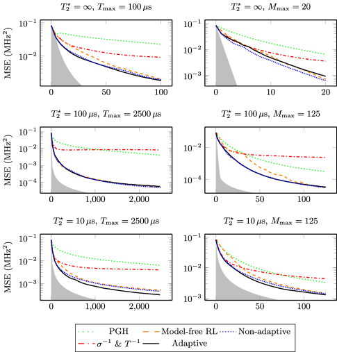
Figure 2: These plots refer to static field magnetometry with an NV center, executed in different conditions. The MSE on $\omega$ is plotted as a function of the total number of consumed resources, which are either the maximum number of measurements $M_{\text{max}}$ or the maximum total free evolution time of the probe, i.e. $T_{\text{max}}\geq\sum_{t=0}^{M-1}\tau_{k}$. The adaptive (NN) and non-adaptive strategies are optimized using model-aware RL. The description of the $\sigma^{-1}\&T^{-1}$ and PGH strategies can be found in the main text. With the label “Model-free RL” we denote the performances obtained in [32] with model-free RL, which are never better than the non-adaptive strategy optimized with our techniques. The shaded grey area represent the (non-tight) ultimate precision bound, computed either from the Cramér-Rao bound or from a bit-counting arguments, see the Supplementary Information Section G.3. The title of each plot contains the transverse relaxation time $T_{2}^{\star}$, which is the time scale of the dephasing noise, along with the maximum amount of resources used in the simulations. The number of particle in the PF was $N=480$ for the first and third rows, and $N=1024$ (left) and $N=1536$ (right) for the second row, which are significantly smaller numbers than the ones used in [32]. The weights and biases of the NN have been initialized randomly, while the initial $\tau$ for the non-adaptive approach is a deterministic linear ramp increasing after each measurement.

For each plot, the best between our optimized adaptive and non-adaptive strategies, outperforms all the other approaches, as illustrated in Fig. 2. There are two comparisons to be made: on one hand we have the optimized adaptive vs. the non-adaptive strategies, which are both original results of this work; on the other hand we have model-free vs model-aware RL, where application of the latter to NV center magnetometry has been studied in [32]. We shall start with the first comparison. Notably, the optimal results for extended coherence times ($T_{2}^{\star}=100\,\mu\text{s},\infty$) are achieved using non-adaptive strategies, which offer several practical advantages in the experimental implementation. Primarily, since the controls are fixed offline before the experiment, there’s no requirement for real-time feedback via rapid electronics. Furthermore, there’s also no need to update the Bayesian posterior on the fly given the absence of adaptivity. Instead, the measurement outcomes can be processed offline, post-measurement, using more powerful hardware. This would significantly reduce online memory usage as there’s no need for real-time updates to the particle filter. In the third row of Fig. 2 we see a gap between the performances of “Adaptive” and “Non-adaptive”, and in [37] we give more examples of the adaptivity being useful. Regarding the second comparison of model-aware and model-free RL, we observe that no strategy trained with model-free RL can beat even the non-adaptive strategy, which means that the results of [32], although close to ours, cannot prove that the NN has been trained to exploit adaptivity, and that it hasn’t simply learned an optimal non-adaptive sequence of measurement times $\tau$. Beside this, we notice that our “Adaptive” strategy and the “Model-free” approach give results that are closer toward the end of the estimation, while they differ for intermediate times. This is due to our use of the cumulative loss. In the simulation with $T_{2}^{\star}=\infty,\,M_{\text{max}}=20$, the NN strategy performs worse than the non-adaptive one because it remains stuck in a local minimum during the training. In Fig. 3 we reported five examples of optimal adaptive trajectories for the estimation of $\omega=0.2\,\text{MHz}$ referring to $T_{\text{2}}^{\star}=10$, together with the optimal non-adaptive strategy. We observe that multiple runs of the agent training will produce consistent performance but not necessarily the same optimized agent. In conclusion we want to put forward an explanation to why the adaptive control seems to give so little advantage with respect to the optimized non-adaptive strategy. For the adaptivity to be advantageous, the phase $\omega\tau$ must be known to some extent. As the error on $\omega$ goes down, the evolution time increases, so that the uncertainty on $\omega\tau$ doesn’t go to zero even after many measurements, which leaves very little room to adaptivity for improving the estimation precision.

Figure 3: Control strategies for the estimation of $\omega$ in DC magnetometry. For the time limited estimation (on the left) five example trajectories produced by the NN are plotted for $\omega=0.2\,\text{MHz}$. On the right, the optimal non-adaptive strategy for the measurement-limited estimation is presented. This prescribes a growing $\tau$ with a random pattern superimposed.

Agnostic Dolinar receiver

Consider the challenge of distinguishing between two known coherent states, $\left|-\alpha\right\rangle$ and $\left|\alpha\right\rangle$, where $\alpha\in\mathbb{R}$ and $\alpha>0$, using a single copy of the signal $\left|\pm\alpha\right\rangle$. The Dolinar receiver optimally addresses this problem through linear optics and photon counting [87, 88, 89, 90, 91, 92, 93]. For this device multiple Machine Learning approaches can be found in the literature [94, 95]. In some recent studies [35, 96], a variant of this device was introduced which doesn’t require a local oscillator (LO) on the receiver side, which must be in phase with the sender’s laser. This is the agnostic Dolinar receiver, in which in place of the LO, $n$ copies of $\left|\alpha\right\rangle$, called the reference states, are sent to the receiver from the sender, alongside the signal $\left|\pm\alpha\right\rangle$. We furthermore assume that classical knowledge about the state $\left|\alpha\right\rangle$ is missing, i.e. $\alpha$ is an unknown parameter of the estimation. In Fig. 4 we represent schematically this device, which leverages the states $\left|\alpha\right\rangle^{\otimes n}$ to perform the discrimination task on the sign of the signal $\left|\pm\alpha\right\rangle$. The signal $\left|\pm\alpha\right\rangle$ enters from the left and is sequentially combined with one of the reference states $\left|\alpha\right\rangle$ on a programmable beam splitter with adjustable reflectivity $\theta_{i}$. At each beam splitter, one of the two ports undergoes measurement by a photon-counter, while the residual signal $\left|\psi_{i}\right\rangle$ from the other port is fed forward to the subsequent beam splitter. The photon counting result is used to update the Bayesian posterior on $\alpha$ and on the signal’s sign, from which the reflectivity for the upcoming beam splitter is determined via a NN. In this task, which is a combination of estimation and discrimination, there are two undetermined parameters: one continuous, i.e. the signal’s amplitude $\alpha\in\mathbb{R}$, and one discrete, i.e. the signal’s sign. The receiver’s performance is assessed based on the error probability in the task of signal classification, with the loss being the one in Eq. 8, while the amplitude $\alpha$ is a nuisance parameter. See [37] for the details about the loss and the input to the NN.

[width=0.9]apparatus_scheme.svg

Figure 4: Schematic representation of the agnostic Dolinar receiver: each thick diagonal line symbolizes a beam splitter with programmable reflectivity $\theta_{i}$. Each “D” device denotes a photon-counter. On the left side of the figure, the building block of this apparatus is illustrated. Here, the input state at step $i$, named $\left|\psi_{i}\right\rangle$, is combined with one of the $n$ training states $\left|\alpha\right\rangle$. One of the two ports undergoes measurement via photon-counting. At the device’s end the second output port is also measured, ensuring no information is left unused.

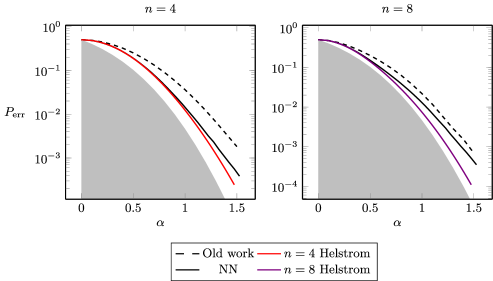
Figure 5: Comparison of error probabilities for various strategies with different numbers of copies of $\left|\alpha\right\rangle$, specifically $n=4$ and $n=8$. The shaded gray area is the region excluded by the Helstrom bound [97, 98], which is the lowest error probability theoretically achievable when assuming having an infinite number of reference states ($n=\infty$) at disposal. The solid red and violet lines are the Helstrom bound calculated for a finite number of copies of $\left|\alpha\right\rangle$ [35], respectively $n=4$ and $n=8$. For the details on the computation of the Helstrom bound see [37]. The black dashed line showcases the lowest error found in the old work [35], without Machine Learning, while the black solid line is the performance achieved using the NN. The performances of the optimal non-adaptive strategies haven’t been reported since they can’t rival the ones of the NN. For both the training and the performances evaluation we used $N=512$ particles. The weights and biases of the NN have been initialized randomly.

The simulation results are presented in Fig. 5. We compared the performances of our adaptive procedure with the current state-of-the-art solution for this problem [35]. In each scenario, we achieved superior results with the NN. Notably, we nearly reached the theoretical bound in our primary area of interest, relevant for long-distance communications, i.e. the full quantum limit with $\alpha\lesssim 1$, and a small number of reference states (specifically, $n=4$). For large $\alpha$, the error probability is already very small and we are in the classical limit.

Choice of the hyperparameters

In this section, we briefly comment on the choice of hyperparameters for the examples reported here. These include the batchsize $B$, the number of particles in the PF $N$, and the initial learning rate $\alpha_{0}$. They must be chosen according to the memory limitations of the computer during training. Specifically, we first empirically fix the number of particles to a value large enough to ensure that the discretization of the posterior does not compromise the precision of the estimation. This, in turn, determines the batchsize, i.e., the number of simulations that can be executed in parallel. The batchsize, along with the type of loss, then determines the initial learning rate. For example, in Fig. 2, we used $B=128$ and $\alpha_{0}=10^{-2}$ for the cumulative loss, as well as $B=1024$ and $\alpha_{0}=10^{-3}$ for the logarithmic loss. These values are used for the time and measurements-limited estimations respectively. The batchsize can also be “artificially” increased via gradient accumulation, which involves averaging the gradients from multiple executions of a batch of simulations for the update in Eq. 12. For the Dolinar receiver, we used $\alpha=10^{-2}$ and $B=4096$. Refer to Appendix E for more information.

III Discussion

Overall, our research highlights the benefits of merging Machine Learning with modern quantum technologies. We introduced a framework, complemented by a versatile library, capable of addressing a wide spectrum of quantum parameter estimation and metrology challenges both in the Bayesian and in the frequentist framework, applicable to a plethora of platforms. Our methods have the potential to accelerate the development of practical applications in quantum metrology. The capability to precisely estimate physical parameters through quantum systems could revolutionize numerous sectors, including biology, fundamental physics, and quantum communication. Through the tool of model-aware reinforcement learning, we aspire to catalyse progress in these domains, smoothing the shift of quantum-based metrology from proof-of-principle experiments to industrial applications. The technique of model-aware RL for agent optimization could be in principle applied to a wide range of problems in quantum information, including quantum error correction and entanglement distillation, which would require engineering other losses. The main obstacle of extending this approach in other fields of quantum information beyond metrology is, however, the exploding dimensionality of the quantum systems states that would need to be simulated.

IV Methods

The library qsensoropt has been implemented in Python 3 on the Tensorflow framework. All of the simulations have been done on the High-Performance Computing cluster of Scuola Normale Superiore. The simulations ran on an NVIDIA Tesla GPU with 32GB of dedicated VRAM. The training and evaluation of each strategy took $\mathcal{O}(1)$ hours.

V Data availability

All the data referenced in this work can be found in the GitLab repository, in the folders qsensoropt/examples/nv_center_dc and qsensoropt/examples/dolinar. The repository can be found at the URL https://gitlab.com/federico.belliardo/qsensoropt.

VI Code availability

The open source library qsensoropt can be found in the GitLab repository and can be installed with pip following the instruction in the README file. The repository can be found at the URL https://gitlab.com/federico.belliardo/qsensoropt.

VII Acknowledgments

We gratefully acknowledge the computational resources of the Center for High Performance Computing (CHPC) at SNS. F. B. thanks T. Shah for useful discussions. We aknowledge finantial support by MUR (Ministero dell’Istruzione, dell’Università e della Ricerca) through the following projects: PNRR MUR project PE0000023-NQSTI, PRIN 2017 Taming complexity via Quantum Strategies: a Hybrid Integrated Photonic approach (QU-SHIP) Id. 2017SRN-BRK. Lastly, this work was supported by the Open Access Publishing Fund of the Scuola Normale Superiore.

VIII Author Contributions

F. Belliardo conceived of the presented idea under the supervision of F. Marquardt and V. Giovannetti. Federico B. and Fabio Z. have programmed the library and performed the simulations, all the authors have discussed the results and contributed to the final manuscript, with F. Belliardo being the main contributor.

IX Competing interests statement

The authors declare no competing interests.

Appendix A Schematization of physical systems in qsensoropt

Encoding of the probe

Following the most common nomenclature in quantum metrology, we will define a quantum probe as a quantum system initialized in a reference state $\rho$. This probe is used to encode the $d$-dimensional vector of parameters $\boldsymbol{\theta}\in\Theta$ of interest, undergoing a controllable evolution, determined by the controls $x$, i.e. $\rho\to\rho_{x,\boldsymbol{\theta}}=\mathcal{E}_{x,\boldsymbol{\theta}}(\rho)$, where $\mathcal{E}_{x,\boldsymbol{\theta}}$ is a general LCPT map. A control is a tunable parameter that can be adjusted during the experiment, this could be for example the measurement duration, the detuning of the laser frequency driving a cavity, or a tunable phase in an interferometer. In a pictorial sense, the control parameters are all the buttons and knobs on the electronics of the experiment. A control can be continuous if it takes values in an interval, or discrete if it takes only a finite set of values (like on and off). The encoded parameters $\boldsymbol{\theta}$ can be a property of the environment, like a magnetic field acting on a spin in the NV center platform, or some degrees of freedom of the probe’s initial state, like the parameter $\alpha$ of a coherent state of light $\left|\alpha\right\rangle$ in the agnostic Dolinar receiver. The same scheme can also be seen as a communication protocol, where Alice sends the state $\rho_{\boldsymbol{\theta}}$ to Bob, which has to decode the $\boldsymbol{\theta}$ vector. We will for the sake of generality call the quantum system probe also in these cases. The idea is to perform a measurement on $\rho_{x,\boldsymbol{\theta}}$ to gain information about $\boldsymbol{\theta}$. An important distinction to be drawn here is that the term quantum parameter estimation refers in the literature to the situation in which we are given the encoded probe $\rho_{\boldsymbol{\theta}}$, in other words, we start from there and we can’t act on the encoding, as opposed to quantum metrology where we are given access to the encoding process $\mathcal{E}_{x,\boldsymbol{\theta}}$ and not only to the final result. The implicit idea in parameter estimation [99] is that the encoding has been carried out outside of the picture. Both in metrology and parameter estimation we assume that the encoding $\mathcal{E}_{x,\boldsymbol{\theta}}$ is applied many times or that we are given many copies of $\rho_{\boldsymbol{\theta}}$, so that we can collect some statistically relevant data by measuring all the copies, from which we infer the value of $\boldsymbol{\theta}$. Quantum metrology is a more general setting than parameter estimation and since the techniques developed here apply to quantum metrology they are also useful for parameter estimation. An example of parameter estimation would be receiving the radiation generated by a distribution of currents on a plane, which depends on the properties of the source, like the temperature for example [56]. In this scenario, the quantum probe is the radiation. Since the emission of the radiation happens by hypothesis in a far and inaccessible region, we don’t have direct access to the quantum channel that performs the encoding, but only to the encoded states, which is the state of the radiated field at detection. An example of a quantum metrological task is the estimation of the environmental magnetic field with a spin, for which we can choose the initial state and the duration of the interaction. A parameter can be continuous or discrete. Naturally continuous parameters are the magnetic field and the temperature, for example. Some examples of discrete parameters are the sign of a signal and the type of the interaction between two quantum systems [100]. When discrete parameters are present, we are in the domain of values discrimination. In a metrological task, we may have a mix of continuous and discrete parameters, like in the agnostic Dolinar receiver of Section II. A parameter can be a nuisance; which is an unknown parameter that needs to be estimated, on which we however do not evaluate the precision of the procedure because we are not directly interested in its value. An example of this is the fluctuating optical visibility of an interferometer when we are only interested in the phase. Estimating the nuisance parameters is often necessary/useful to estimate the parameters of interest.

Measurement on the probe

To obtain some information on $\boldsymbol{\theta}$ it is necessary to perform a measurement on the encoded probe $\rho_{x,\boldsymbol{\theta}}$, which will be represented by a POVM $\mathcal{M}:=\{M_{y}^{x}\}$, where $x$ are the control parameters and $y$ is the measurement outcome. For the purpose of keeping the notation simple we indicate with $x$ both the controls of the evolution and of the measurement. The probability of obtaining $y$ can be computed from the Born rule and it is

$$p(y|\boldsymbol{\theta},x):=\operatorname{tr}\left(M_{y}^{x}\rho_{\boldsymbol{\theta},x}\right)\;.$$ (15)

If the measurement is projective, then we end up in a known state and we have extracted the maximum possible amount of information from $\rho_{x,\boldsymbol{\theta}}$. The probe is then reinitialized in the reference state $\rho$, encoded, and measured again, with the outcome probability given by same expression in Eq. 15. If the measurement is weak (meaning non-projective), then there is still information on $\boldsymbol{\theta}$ encoded in the probe state and we do not reinitialize it. The probe may or may not undergo the evolution $\mathcal{E}_{x^{\prime},\boldsymbol{\theta}}$ again, possibly with different controls $x^{\prime}$. After that the probe is measured again using a different POVM $\mathcal{M}^{\prime}:=\{M^{x^{\prime}}_{y^{\prime}}\}$, leading to the outcome $y^{\prime}$. This procedure can be iterated multiple times, until a projective measurement is performed on the probe, and its state is reinitialized. For a weak measurement the Born rule prescribes an outcome probability that depends on the whole trajectory of previous controls and measurement outcomes. Let us indicate with $\boldsymbol{x}_{t}:=(x_{0},x_{1},\ldots,x_{t})$ and $\boldsymbol{y}_{t}:=(y_{0},y_{1},\ldots,y_{t})$ the tuples containing respectively the controls and outcomes up to the $t$-th iterations. The probability of obtaining $y_{t+1}$ at the $t+1$-th step is

$$p(y_{t+1}|\boldsymbol{x}_{t+1},\boldsymbol{y}_{t},\boldsymbol{\theta}):=\operatorname{tr}\left({M}_{y_{t+1}}^{x_{t+1}}\rho_{\boldsymbol{x}_{t},\boldsymbol{y}_{t},\boldsymbol{\theta}}\right)\;.$$ (16)

The case of a continuous measurement can be simulated by taking the appropriate limits, but it is beyond the scope of this work.

Appendix B Implementation of the particle filter

B.1 Bayesian update

If we perform at each step a projective measurement on the probe, then the probability of observing the outcome $y$, given the control $x$ and the true value $\boldsymbol{\theta}$ of the unknown parameters, is reported in Eq. 4. To recover the value of $\boldsymbol{\theta}$ we apply the principles of Bayesian estimation, that is, starting from the prior $\pi(\boldsymbol{\theta})$ on $\boldsymbol{\theta}$, we calculate the posterior probability distribution with the Bayes rule, i.e.

$$P(\boldsymbol{\theta}|x,y)=\frac{p(y|x,\boldsymbol{\theta})\pi(\boldsymbol{\theta})}{P(y)}=\frac{p(y|x,\boldsymbol{\theta})\pi(\boldsymbol{\theta})}{\int p(y|x,\boldsymbol{\theta})\pi(\boldsymbol{\theta})\mathop{\mathrm{d}\!}{}\boldsymbol{\theta}}\;.$$ (17)

The denominator is just the normalization required for $P(\boldsymbol{\theta}|x,y)$ to be a probability density. For a series of measurements we apply repeatedly the Bayes rule by using the posterior computed at the previous step as the prior of the next one. Given the tuple of controls $\boldsymbol{x}_{t+1}$ and of outcomes $\boldsymbol{y}_{t+1}$, we can compute the posterior at the $t+1$-th step from posterior at the $t$-th step with the formula

$$P(\boldsymbol{\theta}|\boldsymbol{x}_{t+1},\boldsymbol{y}_{t+1})=\frac{p(y_{t+1}|x_{t+1},\boldsymbol{\theta})P(\boldsymbol{\theta}|\boldsymbol{x}_{t},\boldsymbol{y}_{t})}{\int p(y_{t+1}|x_{t+1},\boldsymbol{\theta})P(\boldsymbol{\theta}|\boldsymbol{x}_{t},\boldsymbol{y}_{t})\mathop{\mathrm{d}\!}{}\boldsymbol{\theta}}\;.$$ (18)

Notice that for each measurement the probability of obtaining $y_{t+1}$ as a result is independent on the outcomes and controls up to that point and depends only on $x_{t+1}$. This is precisely because of the reinitialization of the probe after the projective measurements. In order to perform efficiently the Bayesian update on a computer we use the particle filter method (PF), that is, we represent the posterior distribution with a discrete set of points in the space $\Theta$ of the parameters, each with its own weight. Fundamentally this means, we approximate the posterior distribution with a sum of $\delta$-functions, i.e.

$$P(\boldsymbol{\theta}|\boldsymbol{x}_{t},\boldsymbol{y}_{t})\simeq\sum_{j=1}^{N}w_{j}^{t}\delta(\boldsymbol{\theta}-\boldsymbol{\theta}_{j})\;,$$ (19)

where the values $\{\boldsymbol{\theta}_{j}\}_{j=1}^{N}$ are called particles and $\{w_{j}^{t}\}_{j=1}^{N}$ are the weights at the step $t$. The values of the particles are to be sampled from the initial prior $\pi(\boldsymbol{\theta})$, while the weights are initialized uniformly on all the particles, i.e. $\omega_{j}^{0}:=\frac{1}{N}$. The weights depend on the step because of the Bayesian update of the posterior in Eq. 18, which on $w^{t}_{j}$ corresponds to the transformation

$$w_{j}^{t+1}=\frac{p(y_{t+1}|x_{t+1},\boldsymbol{\theta}_{j})w_{j}^{t}}{\sum_{j=1}^{N}p(y_{t+1}|x_{t+1},\boldsymbol{\theta}_{j})w_{j}^{t}}\;,$$ (20)

The particles $\{\boldsymbol{\theta}_{j}\}_{j=1}^{N}$ should also depend on the step $t$, in fact we will introduce a resampling procedure that when triggered generates a new set of particles, which therefore don’t necessarily remain unvaried along the estimation. Nevertheless for notational simplicity we avoid putting a time index on $\boldsymbol{\theta}_{j}$. We indicate to the set of particles and the weights with $\mathfrak{p}_{t}:=\{\boldsymbol{\theta}_{j},w_{j}^{t}\}_{j=1}^{N}$, which we call the PF ensemble.

B.2 Moments of the posterior

Computing the first moments of the posterior (the mean value and the covariance matrix) corresponds to simple linear algebra operations on the PF ensemble, i.e.

$$\boldsymbol{\widehat{\theta}}_{t}:=\int\boldsymbol{\theta}P(\boldsymbol{\theta}|\boldsymbol{x}_{t},\boldsymbol{y}_{t})\mathop{\mathrm{d}\!}{}\boldsymbol{\theta}\simeq\sum_{j=1}^{N}w_{j}^{t}\boldsymbol{\theta}_{j}\;,$$ (21)

and

$$\Sigma_{t}:=\int(\boldsymbol{\theta}-\boldsymbol{\widehat{\theta}}_{t})(\boldsymbol{\theta}-\boldsymbol{\widehat{\theta}}_{t})^{\intercal}P(\boldsymbol{\theta}|\boldsymbol{x}_{t},\boldsymbol{y}_{t})\mathop{\mathrm{d}\!}{}\boldsymbol{\theta}\simeq\sum_{j=1}^{N}w_{j}^{t}(\boldsymbol{\theta}_{j}-\boldsymbol{\widehat{\theta}}_{t})(\boldsymbol{\theta}_{j}-\boldsymbol{\widehat{\theta}}_{t})^{\intercal}\;.$$ (22)

The mean value of the posterior $\boldsymbol{\widehat{\theta}}$ is our estimator for all continuous parameters throughout the paper. As the estimation proceeds the weights typically concentrate on few particles, while all the others do not play any role in the estimation if not consuming memory. The precision is limited by the average distance between the points $\boldsymbol{\theta}_{j}$, which depends on the prior $\pi(\boldsymbol{\theta})$ and on the number of particles $N$. We see in the next section how the introduction of a resampling scheme can mitigate this issue by extracting a new set of particles $\{\boldsymbol{\theta}_{j}^{\prime}\}_{j=1}^{N}$ , which should be in the region where the posterior distribution is concentrated. This means that the density of particles in this region increases allowing for more resolution in distinguishing close values of $\boldsymbol{\theta}$. Throughout the paper we use the same symbols for the “theoretical” moments of the posterior (which are not accessible) and the approximation of these quantities computed from the PF. It will be clear from the contex which quantities we are referencing when.

B.3 Resampling scheme

While for a small number of unknown parameters we could still obtain good performances even if no resampling procedure is performed, it is essential for larger dimensions. Indeed the density of particles, i.e. the resolution in $\boldsymbol{\theta}$, after the initialization, is inversely proportional to the volume of the parameter space, which grows exponentially in the number $d$ of dimension of the $\Theta$ space. To solve this problem it is typical to perform during the estimation a resampling of the particles according to the posterior distribution, which is triggered by the condition

$$N_{\text{eff}}:=\frac{1}{\sum_{j=1}^{N}(w_{j}^{i})^{2}}<r_{t}N\;,$$ (23)

where $r_{t}$ is the resampling threshold that is kept fixed at $r_{t}=0.5$ in all the simulations of the paper. The left hand side of Eq. 23 is sometimes called the effective number of particles $N_{\text{eff}}$.

Soft resampling

The simplest resampling scheme prescribes the extraction of $N$ samples with repetitions from the set of indexes $J=\{1,\cdots,N\}$, each weighted with the corresponding $w_{j}$, $j\in J$. We will call $\phi(j):J\rightarrow J$ the map that gives the outcome of the $j$-th extraction event. The indexes $j\in J$ corresponding to the particles $\boldsymbol{\theta}_{j}$ that have large weights are extracted more frequently, while the particles with small weights tend to disappear. In our implementation we considered a slightly more general version of this procedure which goes under the name of soft resampling [64], that is, we mix the probability distribution represented by the weights $\{w_{j}\}_{j=1}^{N}$ with a uniform distribution on $\{\boldsymbol{\theta}_{j}\}_{j=1}^{N}$ by constructing the soft-weights $q_{j}$ defined as

$$q_{j}:=\alpha w_{j}+(1-\alpha)\frac{1}{N}\;,$$ (24)

where $\alpha\in[0,1]$ is a parameter characterizing the effectiveness of the resampling. With $\alpha=1$ we have the traditional procedure, while with $\alpha=0$ no actual resampling is performed, because we extract the new particles from a uniform distribution, just like at the beginning. With $\alpha=0$ the particles with low weights are not cut away from the ensemble but persist after the process. With an intermediate value of $\alpha$ (by default we set $\alpha=0.5$) only a fraction $\alpha$ of the particles are effective for the resampling, because the other fraction $(1-\alpha)$ is expected to be distributed uniformly. We call $\boldsymbol{\theta}_{j}^{\prime}$ the new particles extracted from $q_{j}$, i.e.

$$\boldsymbol{\theta}_{j}^{\prime}=\boldsymbol{\theta}_{\phi(j)}\;.$$ (25)

Their corresponding weights are chosen, so that the ensemble of the PF represents the same distribution as before the resampling. These are

$$w^{\prime}_{j}\propto\frac{w_{\phi(j)}}{q_{\phi(j)}}=\frac{w_{\phi(j)}}{\alpha w_{\phi(j)}+(1-\alpha)\frac{1}{N}}\;,$$ (26)

that still need to be normalized. With this choice for $w^{\prime}_{j}$ the PF represents the correct posterior even though the particles have been sampled from a different distribution. The probability density function represented by the PF is, roughly speaking, proportional to the product of the weights $w_{j}^{\prime}$ and the density of particles at the position $\boldsymbol{\theta}_{j}^{\prime}$, i.e. $q_{\phi(j)}$, which with our choice for $w_{j}^{\prime}$ is exactly $w_{\phi(j)}$, i.e. the weight of the particle $\boldsymbol{\theta}_{j}^{\prime}$ prior to the resampling step. In the next section we detail this relation. The reader that is interested in the successive steps of the resampling can however skip it. The soft resampling scheme, which is based on importance sampling [101], will be crucial in making the PF differentiable [102, 103]. We might want, in general, to perform a subsampling of the particles, that is, we sample from the distribution in Eq. 24 not $N$ but $\gamma N$ particles, with $0<\gamma\leq 1$. We will later in the resampling routine propose $(1-\gamma)N$ new particles that will help us in representing the posterior better, so that we have in total after the resampling step $N$ particles again. In this case the weights in Eq. 26 will be normalized as $w_{j}^{\prime}\rightarrow\frac{w_{j}^{\prime}}{\mathcal{C}}$, where $\mathcal{C}$ is such that

$$\frac{1}{\mathcal{C}}\sum_{j=1}^{\gamma N}w_{j}=\gamma\;,$$ (27)

By default we set $\gamma=0.99$, that is, only $1\%$ of the particles after the resampling are new.

Particle filters and importance sampling

In this section we review the core ideas underlying the functioning of a particle filter and the principle of importance sampling, as it is applied in our implementation of the soft resampling. Consider a distribution $P(\boldsymbol{\theta})$, from which we sample $N$ particles $\boldsymbol{\theta}_{j}$ with $j=1,\cdots,N$. Let us define an hypercube $\mathcal{C}$ of volume $\mathop{\mathrm{d}\!}{}\boldsymbol{\theta}$ centred around $\boldsymbol{\theta}$, and let us call $n(\boldsymbol{\theta},d^{N}\boldsymbol{\theta})$ the number of particles in the said hypercube, i.e.

$$n(\boldsymbol{\theta},\mathop{\mathrm{d}\!}{}\boldsymbol{\theta}):=\sum_{j=1}^{N}\chi_{\mathcal{C}}(\boldsymbol{\theta}_{j})\;$$ (28)

with $\chi_{\mathcal{C}}$ being the characteristic function of the hypercube. We can write

$$\frac{1}{N}n(\boldsymbol{\theta},d^{N}\boldsymbol{\theta})\rightarrow P(\boldsymbol{\theta})\mathop{\mathrm{d}\!}{}\boldsymbol{\theta}\quad\text{for}\;N\rightarrow\infty\;,$$ (29)

that is in the limit of large $N$ the fraction of particles in the hypercube tends to the probability in such volume element. In a PF we associate to each particle $\boldsymbol{\theta}_{i}$ a weight $w_{i}$ and we can define the total weight in the hypercube $\mathcal{C}$ as

$$P(\boldsymbol{\theta})\mathop{\mathrm{d}\!}{}\boldsymbol{\theta}\simeq w(\boldsymbol{\theta},d^{N}\boldsymbol{\theta}):=\sum_{j=1}^{N}w_{j}\chi_{\mathcal{C}}(\boldsymbol{\theta}_{j})\;.$$ (30)

This total weight is the probability distribution actually represented by the PF. In the limit of large $N$, for a smooth distribution, we can consider the weight a function of the point $w(\boldsymbol{\theta})$, which varies smoothly in space and is approximatively constant in the hypercube $\mathcal{C}$. This leads us to write

$$P(\boldsymbol{\theta})\mathop{\mathrm{d}\!}{}\boldsymbol{\theta}\simeq w(\boldsymbol{\theta})\sum_{j=1}^{N}\chi_{\mathcal{C}}(\boldsymbol{\theta}_{j})=w(\boldsymbol{\theta})n(\boldsymbol{\theta},\mathop{\mathrm{d}\!}{}\boldsymbol{\theta})\;.$$ (31)

This means that the distribution represented by the particle filter is proportional to the product of the weights and the density of the particles. This is however not the only way to represent $P(\boldsymbol{\theta})$. Suppose that for whatever reason we sample the particles $\boldsymbol{\theta}_{j}$ from $Q(\boldsymbol{\theta})$, but that we actually want to represent the distribution $P(\boldsymbol{\theta})$. Then we can multiply the weights $w_{j}=1/N$ of each particle $\boldsymbol{\theta}_{j}$ with the corrective factor $P(\boldsymbol{\theta}_{j})/Q(\boldsymbol{\theta}_{j})$, which remains approximately constant inside the region $\mathcal{C}$, i.e.

$$w(\boldsymbol{\theta},d^{N}\boldsymbol{\theta})=\frac{1}{N}\sum_{j=1}^{N}\frac{P(\boldsymbol{\theta}_{j})}{Q(\boldsymbol{\theta}_{j})}\chi_{\mathcal{C}}(\boldsymbol{\theta}_{j})\simeq\frac{P(\boldsymbol{\theta})}{Q(\boldsymbol{\theta})}\frac{1}{N}\sum_{j=1}^{N}\chi_{\mathcal{C}}(\boldsymbol{\theta}_{j})=\frac{P(\boldsymbol{\theta})}{Q(\boldsymbol{\theta})}\frac{n(\boldsymbol{\theta},d^{N}\boldsymbol{\theta})}{N}\;,$$ (32)

since now the particles are distributed spacially according to $Q(\boldsymbol{\theta})$ the density of particles will tend to $Q(\boldsymbol{\theta})$ for large $N$ that, according to Eq. 29, gives $w(\boldsymbol{\theta},d^{N}\boldsymbol{\theta})\rightarrow Q(\boldsymbol{\theta})$, therefore we have $w(\boldsymbol{\theta},d^{N}\boldsymbol{\theta})\simeq P(\boldsymbol{\theta})$. In the case of soft resampling the distribution $Q(\boldsymbol{\theta})$ is constructed from $P(\boldsymbol{\theta})$ as

$$Q(\boldsymbol{\theta})\mathop{\mathrm{d}\!}{}\boldsymbol{\theta}:=\left[\alpha w(\boldsymbol{\theta})+(1-\alpha)\frac{1}{N}\right]n(\boldsymbol{\theta},\mathop{\mathrm{d}\!}{}\boldsymbol{\theta})\;,$$ (33)

and the factor that multiplies the weights is $P(\boldsymbol{\theta})/Q(\boldsymbol{\theta})=w(\boldsymbol{\theta})/\left[\alpha w(\boldsymbol{\theta})+(1-\alpha)\frac{1}{N}\right]$. The factor used in Eq. 26 for the particle at $\boldsymbol{\theta}_{j}^{\prime}$ contains $w_{\phi}(j)$ , which is the weight at this point in the original distribution $P(\boldsymbol{\theta})$.

Gaussian perturbation

After the soft resampling we add a perturbation to the particles as proposed in [73], that is, we define

$$\boldsymbol{\theta}_{j}^{\prime\prime}:=\beta\boldsymbol{\theta}_{j}^{\prime}+(1-\beta)\boldsymbol{\widehat{\theta}}_{t}+\boldsymbol{\delta}\;,$$ (34)

where $\beta\in(0,1]$, $\boldsymbol{\widehat{\theta}}_{t}$ is the mean of the posterior approximated in Eq. 21 and $\boldsymbol{\delta}$ is a random variable distributed according to

$$\boldsymbol{\delta}\sim\mathcal{N}(0,(1-\beta^{2})\Sigma_{t})\;.$$ (35)

With this expression we move the particles toward the mean of the posterior, which is our estimator for $\boldsymbol{\theta}$ and at the same time we lift the degeneracy of the $\boldsymbol{\theta}_{j}^{\prime}$, that comes about because the particle $\boldsymbol{\theta}_{j}$ with high weights appear many times in the new particles ensemble. Were the degeneracy not removed, all these copies of the same particle wouldn’t contribute much to improve resolution of the PF. This holds true unless they are perturbed, at which point they can encode the small scale behaviour of the posterior. Because of the perturbation in Eq. 34 the PF does not represent anymore the posterior $P(\boldsymbol{\theta}|\boldsymbol{x}_{t},\boldsymbol{y}_{t})$ exactly. We now compute the probability distribution for $\boldsymbol{\theta}_{j}^{\prime\prime}$ after the perturbation step. The particles are distributed in the space according to the $q_{j}$ weights in Eq. 24 and we call this distribution $Q(\boldsymbol{\theta}^{\prime})$. Let us write Eq. 34 as $\boldsymbol{\theta}_{j}^{\prime\prime}=\beta\boldsymbol{\theta}_{j}^{\prime}+\boldsymbol{\delta}^{\prime}$ with

$$\boldsymbol{\delta}^{\prime}\sim\mathcal{N}((1-\beta)\boldsymbol{\widehat{\theta}}_{t},(1-\beta^{2})\Sigma_{t})\;,$$ (36)

being a perturbation with non-null mean value. Then the probability density for $\boldsymbol{\theta}_{j}^{\prime\prime}$ is the convolution of the probability of a particle being at position $\boldsymbol{\theta}^{\prime}$ and the probability of the noise causing a displacement $\boldsymbol{\delta}^{\prime}=\boldsymbol{\theta}^{\prime\prime}-\beta\boldsymbol{\theta}^{\prime}$, i.e.

$$\widetilde{Q}(\boldsymbol{\theta}^{\prime\prime})=\int Q(\boldsymbol{\theta}^{\prime})g_{\beta}(\boldsymbol{\theta}^{\prime\prime}-\beta\boldsymbol{\theta}^{\prime})\mathop{\mathrm{d}\!}{}\boldsymbol{\theta}^{\prime}=\sum_{j=1}^{\gamma N}q_{\phi(j)}g_{\beta}(\boldsymbol{\theta}^{\prime\prime}-\beta\boldsymbol{\theta}^{\prime}_{j})\;,$$ (37)

where $g_{\beta}$ is the Gaussian probability density associated to $\boldsymbol{\delta}^{\prime}$, i.e.

$$g_{\beta}(\boldsymbol{\theta}):=(2\pi)^{-\frac{\mathop{\mathrm{d}\!}{}}{2}}(1-\beta^{2})^{-\frac{1}{2}}\det(\Sigma_{t})^{-\frac{1}{2}}\exp\left[-\frac{1}{2(1-\beta^{2})}\left(\boldsymbol{\theta}-(1-\beta)\boldsymbol{\widehat{\theta}}_{t}\right)^{\intercal}\Sigma_{t}^{-1}\left(\boldsymbol{\theta}-(1-\beta)\boldsymbol{\widehat{\theta}}_{t}\right)\right]\;.$$ (38)

In Eq. 37 we also substituted the integral with a summation being the probability $Q(\boldsymbol{\theta}^{\prime})$ discrete. According to the principles of importance sampling the distribution represented by a PF is the product of the weights and the density of particles, which reads

$$\widetilde{P}(\boldsymbol{\theta}_{j})\propto\frac{P(\boldsymbol{\theta})}{Q(\boldsymbol{\theta})}\widetilde{Q}(\boldsymbol{\theta}_{j})\simeq P(\boldsymbol{\theta})\;,$$ (39)

In principle we could correct the distribution for this perturbation by computing exactly Eq. 37 and accounting for it in the weights $w_{j}^{\prime}$, in our implementation we don’t do it however, since it would be very small anyway.

New particles proposal

We still need to produce $(1-\gamma)N$ new particles and we do it by extracting them from the Gaussian distribution with the same two first moments of the PF ensemble, i.e.

$$\boldsymbol{\theta}_{j}^{{}^{\prime\prime}}\sim\mathcal{N}\left(\boldsymbol{\widehat{\theta}},\Sigma\right)\;,$$ (40)

for $j=\gamma N,\cdots,N$. The mean and the covariance matrix are defined in Eq. 21 and Eq. 22 respectively. This is done again to increase the density of particles in the region of high probability, but it works properly only for unimodal distributions. The weights of these new particles are set to $w_{j}^{\prime}=\frac{1}{N}$, so that their normalization is

$$\sum_{j=\gamma N}^{N}w^{\prime}_{j}=1-\gamma\;.$$ (41)

This extra particles and weights are concatenated directly to $\{\boldsymbol{\theta}_{j}^{\prime\prime}\}_{j=1}^{\gamma N}$ and $\{w_{j}^{\prime}\}_{j=1}^{\gamma N}$. We then rename the new weights and particles, i.e. $w_{j}^{\prime}\rightarrow w_{j}$ and $\boldsymbol{\theta}^{\prime\prime}_{j}\rightarrow\boldsymbol{\theta}_{j}$, and with that the resampling procedure is concluded. In doing the last step of proposing new particles we are mixing the distribution represented by the PF $P(\boldsymbol{\theta})$ as it comes out of the perturbation step in Eq. 39 with the distribution $g_{0}$ in Eq. 38. At the end the PF ensemble represents the distribution

$$P^{\prime}(\boldsymbol{\theta})=\gamma P(\boldsymbol{\theta})+(1-\gamma)g_{0}(\boldsymbol{\theta})\;.$$ (42)

Again we do not correct for this distortion, which could be done by modifying the weights properly.

Resampling of the batch

In order to compute the precision of the estimation, we need the results of many runs of the simulation, possibly executed in parallel on a GPU. In these circumstances the resampling is performed on all the instances of the estimation as soon as the condition Eq. 40 holds true for at least a fraction $f$ of the estimations in the batch, which by default is set to $f=0.98$. The premature resampling of an estimation run will have a quite strong detrimental effect on the goodness of the posterior represented by the PF, on the contrary a late resampling is much less probable to distort the distribution, this is the reason why we set $f$ so close to one, that is, we want to limit as much as possible the number of simulations that are prematurely resampled. With the current implementation at each step either all the simulations is the batch are resampled or none. An improvement to the PF would be to resample selectively only those runs that are in need of resampling, and leave the other untouched until they satisfy Eq. 40, so that whatever number of runs could be resampled at each step. The complete resampling cycle, including the extraction and the new particle and the importance sampling is represented in Fig. 6.

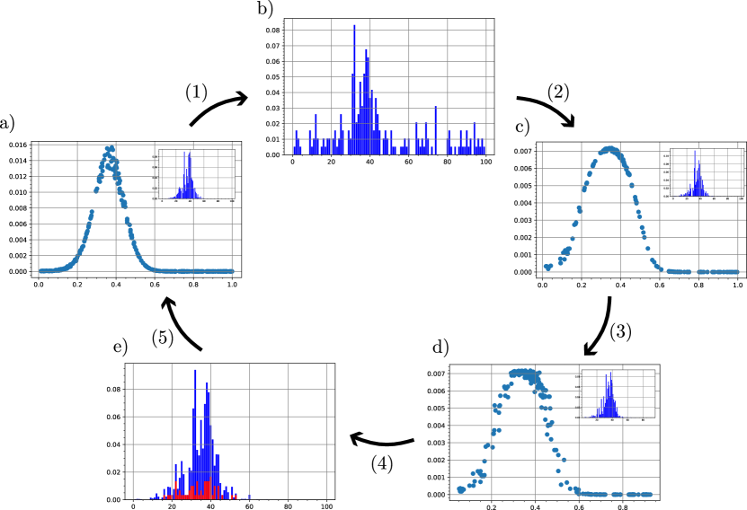
Figure 6: The ensemble of the PF before the resampling is represented in a), the scatter plot are the points $(\boldsymbol{\theta}_{j},w_{j})$. This plot doesn’t represent directly the posterior, because it doesn’t take into account the density of particles. In all the plots, the inserted histogram is the actual posterior represented by the PF. Once the condition Eq. 23 is satisfy the first step of the resampling is executed, which is the transformation (1) and corresponds to sampling with repetitions from Eq. 24, the plot b) is the spatial density of particles after this action. The scatter plot c) is the distribution of the PF after the weights have been corrected according to Eq. 26 (transformation (2)). (3) is the application of the Gaussian noise in Eq. 34 and (4) is the sampling of the extra proposed particles in Eq. 40. Plot e) is the distribution represented by the PF when the resampling routine is complete, where in red the contribution of the new particles is highlighted. At last (5) is the repeated application of the Bayes rule Eq. 20, following some new measurement on the probe, that leads to the ensemble of the PF being again in need of resampling. To emphasise the effect of each transformation we have set $\alpha=0.5,\beta=0.9,\gamma=0.8$. The total number of particles was $N=10^{3}$ and the effective number of particles in a), that is before the resampling, was $N_{\text{eff}}=93.8$. In the histograms the interval $[0,1]$ of the scatter plots has been mapped to $[0,100]$.

B.4 State particle filter

In this section we describe what happens when we are acting with weak (non-projective) measurements on the probe. In this case the probability to observe the outcome $y_{t+1}$ at the step $t+1$ depends on all the string of previous outcomes and controls, that is on the whole trajectory $\tau:=(\boldsymbol{x}_{t},\boldsymbol{y}_{t})$, as well as on the current control $x_{t+1}$. This means we must substitute $p(y_{t+1}|x_{t+1},vtheta)$ with $p(y_{t+1}|\boldsymbol{\theta},\boldsymbol{x}_{t+1},\boldsymbol{y}_{t})$ in Eq. 20. Since we avoid the reinitialization of the probe, its state depends on all the evolution history. With this change in the outcome probability all the formulas of the previous section remain valid. To compute $p(y_{t+1}|\boldsymbol{\theta},\boldsymbol{x}_{t+1},\boldsymbol{y}_{t})$, we need to keep track of the state of the probe. In order to do so we introduce the state particle filter. In this data structure we save for each particle $\boldsymbol{\theta}_{j}$ the state of probe had the system evolved under the action of $\mathcal{E}_{\boldsymbol{\theta}_{j},x}$, with the controls and the outcomes being the ones actually applied/observed in the evolution, we indicate this state with $\rho_{\boldsymbol{\theta}_{j},\tau_{t}}$. To this state we associate the weight $w_{j}$ of the particle $\boldsymbol{\theta}_{j}$. The state particle filter represents the posterior probability distribution for the state of the probe conditioned on the trajectory $\tau_{t}$. The expression for $\rho_{\boldsymbol{\theta}_{j},\tau_{t}}$ reads

$$\rho_{\boldsymbol{\theta}_{j},\tau_{t}}=\mathcal{M}_{y_{t}}^{x_{t}}\circ\mathcal{E}_{\boldsymbol{\theta}_{j},x_{t}}\circ\mathcal{M}_{y_{t-1}}^{x_{t-1}}\circ\mathcal{E}_{\boldsymbol{\theta}_{j},x_{t-1}}\circ\cdots\circ\mathcal{M}_{y_{1}}^{x_{1}}\circ\mathcal{E}_{\boldsymbol{\theta}_{j},x_{1}}(\rho)\;,$$ (43)

where

$$\mathcal{M}_{y_{t}}^{x_{t}}(\rho):=\frac{M_{y_{t}}^{x_{t}}\rho M_{y_{t}}^{x_{t}\dagger}}{\operatorname{tr}\left[M_{y_{t}}^{x_{t}}\rho M_{y_{t}}^{x_{t}\dagger}\right]}\;,$$ (44)

is the backreaction of the measurement on the state of the probe. The estimator for the probe state at the step $t$ is

$$\widehat{\rho}_{\tau_{t}}:=\sum_{j=1}^{N}w_{j}\rho_{\boldsymbol{\theta}_{j},\tau_{t}}\;,$$ (45)

that is, the mean of the state on the posterior distribution for the parameters. The estimator $\widehat{\rho}_{\tau_{t}}$ can then be fed to the agent, to contribute to the computation of the next control. When the resampling is performed on the PF ensemble we get a new set of particles $\boldsymbol{\theta}_{j}^{\prime}$ and their corresponding states must be also updated. This means we have to keep track of the vectors $\boldsymbol{x}_{t}$ and $\boldsymbol{y}_{t}$ in the simulations and recompute the evolution of the whole state particle filter from the beginning, so that we get $\rho_{\boldsymbol{\theta}_{j}^{\prime},\tau_{t}}$. From the computational point of view, the fact that we need these rather memory intensive structures of the PF and the state PF tells us that the optimization loop presented here can be applied only to rather small and simple quantum sensors.

B.5 Multimodal posterior distributions

The resampling procedure presented in the previous section has some limitation in dealing with multimodal distributions. In this case the mean of the posterior may lay in a region of relatively low probability between two peaks and the accumulation of particles in this region after a resampling would be detrimental to the precision of the estimation. From its own design it would be difficult to modify the PF so that it accounts for multiple maxima. The informations that we can easily extract from the PF are its moments and from them the actual positions of the maxima are not straightforward to obtain. Multimodal posterior distributions are however common in quantum metrology. For example in multiphase estimation, like the measurement of the hyperfine interaction in NV-${}^{13}C$. To promote the preservation of secondary features in the posterior distribution we can use multiple particle filter at once. In this situation a set of PFs, with different priors, are updated in parallel and only together represent the full Bayesian posterior. To reduce the memory requirement of such approach we could consider simple Gaussian distributions instead of full PFs. We start by approximating the prior distribution $\pi(\boldsymbol{\theta})$ with as a sum of $L$ Gaussians:

$$\pi(\boldsymbol{\theta})\simeq\sum_{l=1}^{L}w_{l}\mathcal{N}(\boldsymbol{\mu}_{l},\boldsymbol{\sigma}_{l})\;.$$ (46)

If the parameters $\boldsymbol{\mu}_{l},\boldsymbol{\sigma}_{l}$ are fixed then the Bayesian update step can be done by solving a linear regression problem to find the best new values for $\{w_{l}\}_{l=1}^{L}$ that represent the posterior. In this way the PF has however a limited resolution, determined by the initial Gaussian. If we also let $\boldsymbol{\mu}_{l},\boldsymbol{\sigma}_{l}$ change during the Bayesian update step, then we solve the problem of having limited resolution, but we now have to deal with a non-linear regression problem.

Appendix C Differentiability of the particle filter

In this section we discuss what happens when the resampling routine of the particle filter is switched on, and, in particular, what we need to do to assure that the gradient produced by the automatic differentiation is correct.

C.1 Differentiable PF through reparametrization and soft resampling

Differentiability of the soft resampling

As seen in Section D.3, the gradient can’t be propagated through randomly extracted variables, therefore when the categorical resampling is executed, the particles $\boldsymbol{\theta}_{j}^{\prime}$ in Eq. 25 don’t have any connection with the controls, i.e.

$$\frac{\mathop{\mathrm{d}\!}{}\boldsymbol{\theta}_{j}^{\prime}}{\mathop{\mathrm{d}\!}{}\boldsymbol{\lambda}}=0\;.$$ (47)

Similarly, the weights are reinitialized and loose every dependence on the history of the estimation. At the moment of taking the gradient we won’t be able to account for anything that happened before the last resampling. This means that the training routine optimizes the agent only for the later steps, although what has been learnt in this context may be useful also for the earlier measurements. The soft resampling with $\alpha<1$, introduced in Appendix B, is able to partially remove this obstacle. With this trick the dependence on $\boldsymbol{\lambda}$ is passed from the old weights to the new ones through Eq. 26. However, the gradient doesn’t backpropagate entirely but it is attenuated by the factor $1-\alpha$. The price to pay for propagating the gradient is that the $N$ particles are not all fully effective for the resampling, instead only a fraction $\alpha$ of them participate to it. As discussed in Section D.3, since we are extracting stochastic variables from the distribution in Eq. 24, we should also add the corresponding log-likelihood terms $\sum_{j}\log q_{\phi(j)}$ to the loss. However adding so many terms would increase too much the variance of the gradient. Either we don’t account for these log-likelihoods and we accept the gradient to have a bias, or we use the correction introduced in [29], that prescribes to substitute the definition of the new weights $w_{j}^{\prime}$ with an appropriate surrogate expressions. Introducing this correction is the default behaviour of our code but it can be applied only if the loss $\ell(\boldsymbol{\widehat{\theta}},\boldsymbol{\theta})$ is of a certain form. It can be proved that for the MSE defined in Eq. 7 this gives the correct gradient. See Section C.2 for a complete discussion.

Differentiability of the perturbation

The next transformation on the particles is the perturbation of Eq. 34. Again we would be unable to propagate the gradient through the perturbation $\boldsymbol{\delta}^{\prime}$, if we extracted it directly from the Gaussian $\mathcal{N}(\boldsymbol{\mu},\Sigma)$, with $\boldsymbol{\mu}=(1-\beta)\boldsymbol{\widehat{\theta}}_{t}$ and $\Sigma=(1-\beta^{2})\Sigma_{t}$. For this reason we apply the reparametrization trick and write

$$\boldsymbol{\delta}^{\prime}(\boldsymbol{y}_{t},\boldsymbol{\lambda})=\Sigma(\boldsymbol{y}_{t},\boldsymbol{\lambda})\boldsymbol{u}+\boldsymbol{\mu}(\boldsymbol{y}_{t},\boldsymbol{\lambda})\;,$$ (48)

where $\boldsymbol{u}$ is extracted from the multivariate standard Gaussian $\boldsymbol{u}\sim\mathcal{N}(0,\mathbbm{1})$. The perturbation is now a differentiable functions of $\boldsymbol{\lambda}$. For the extraction of $\boldsymbol{u}$ we do not need to add a corresponding log-likelihood term, as discussed in Section D.3, because its probability density function doesn’t depend on $\boldsymbol{\lambda}$.

Differentiability of the proposed particles

For the last step of the resampling, which consists in proposing new particles $\boldsymbol{\theta}_{j}^{\prime\prime}$, extracted from $\mathcal{N}(\boldsymbol{\widehat{\theta}}_{t},\Sigma_{t})$, we again exploit the reparametrization trick and write

$$\boldsymbol{\theta}_{j}^{\prime\prime}(\boldsymbol{y}_{t},\boldsymbol{\lambda})=\Sigma_{t}(\boldsymbol{y}_{t},\boldsymbol{\lambda})\boldsymbol{u}_{j}+\boldsymbol{\widehat{\theta}}_{t}(\boldsymbol{y}_{t},\boldsymbol{\lambda})\;,$$ (49)

which is again differentiable and doesn’t require a log-likelihood term.

Differentiability of the state particle filter

Regarding the differentiability of the state particle filter discussed in Section B.4, we observe that its elements are functions of $\boldsymbol{\lambda}$ through the trajectory $\tau_{t}(\boldsymbol{\lambda})=(\boldsymbol{x}_{t}(\boldsymbol{y}_{t},\boldsymbol{\lambda}),\boldsymbol{y}_{t})$:

$$\rho_{j}(\boldsymbol{\lambda}):=\rho_{\boldsymbol{\theta}_{j},\tau_{t}(\boldsymbol{\lambda})}\;.$$ (50)

Under the assumption that the encoding and the measurements appearing in Eq. 43 are differentiable we can propagate the gradient through the evolution of the probe in Eq. 43 . When the particles are resampled and the new states are computed, the dependence of the new state $\rho_{j}(\boldsymbol{\lambda})$ on the old weights of the PF, and therefore on $\boldsymbol{\lambda}$, persists through the measurement backreaction operators $\mathcal{M}_{x_{t}(\boldsymbol{\lambda})}^{y_{t}}$. A new dependence on $\boldsymbol{\lambda}$ appears in the evolution map $\mathcal{E}_{\boldsymbol{\theta}_{j}(\boldsymbol{\lambda}),x_{t}(\boldsymbol{\lambda})}$, coming from the new particles $\boldsymbol{\theta}_{j}(\boldsymbol{\lambda})$, so that we can write

$$\rho_{j}^{\prime}(\boldsymbol{\lambda}):=\rho_{\boldsymbol{\theta}_{j}(\boldsymbol{\lambda}),\tau_{t}(\boldsymbol{\lambda})}\;.$$ (51)

C.2 Differentiable PF through the correction of Ścibior and Wood

In [29] a correction was introduced to make the resampling procedure in a PF differentiable. This can be implemented in place of the soft resampling, or alongside with it. The default behaviour of our software is to perform the soft resampling with $\alpha=0.5$ alongside the Ścibor and Wood correction. With this choice only half of the gradient is backpropagated through soft resampling, the other half is done by the Ścibor and Wood correction. The former prescribes to modify the normalized weights $w_{j}^{\prime}$ of Eq. 26 to

$$\widetilde{w}_{j}^{\prime}\leftarrow w_{j}^{\prime}\frac{q_{\phi(j)}}{\text{sg}\left[q_{\phi(j)}\right]}\;,$$ (52)

where the meaning of the symbols is that of Section B.3. In this formula we are using the stop gradient operator $\text{sg}\left[\cdot\right]$, which is an instruction that tells the automatic differentiation frameworks not to compute the derivatives of the expression inside the operator. This correction has no effects in the forward pass, but produces additional gradient terms in the backward pass. We see in this section, that for a MSE loss the extra terms in the gradient appearing because of this surrogate expression are exactly the log-likelihoods that we would have to insert following the conclusions of Section D.3, although this observation can’t be extended to a generic loss. Let us start from the expression for the MSE, when one and only one resampling is performed in the whole experiment, at step $t$, i.e.

$$\Delta^{2}\boldsymbol{\widehat{\theta}}=\int\ell(\boldsymbol{\widehat{\theta}},\boldsymbol{\theta})P(\tau_{t+1:M-1}|\boldsymbol{\theta}_{j}^{\prime},\boldsymbol{\theta})\left(\prod_{j=1}^{N}P(\boldsymbol{\theta}_{j}^{\prime}|\tau_{0:t})\right)P(\tau_{0:t}|\boldsymbol{\theta})\pi(\boldsymbol{\theta})\mathop{\mathrm{d}\!}{}\tau_{M-1}\left(\prod_{j=1}^{N}\mathop{\mathrm{d}\!}{}\boldsymbol{\theta}_{j}^{\prime}\right)\mathop{\mathrm{d}\!}{}\boldsymbol{\theta}\;.$$ (53)

We assume for clarity that the perturbation and the extraction of the extra particles, in Eq. 48 and Eq. 49 respectively, are turned off, i.e. $\beta=\gamma=1$. The object $\tau_{\alpha:\beta}$ with $\alpha,\beta$ integers in $[0,M-1]$ is the trajectory between the steps $\alpha$ and $\beta$ (extrema included), i.e. $\tau_{\alpha:\beta}=(\boldsymbol{x}_{\alpha:\beta},\boldsymbol{y}_{\alpha:\beta})$ with $\boldsymbol{x}_{\alpha:\beta}=(x_{\alpha},x_{\alpha+1},\ldots,x_{\beta})$ and $\boldsymbol{y}_{\alpha:\beta}=(y_{\alpha},y_{\alpha+1},\ldots,y_{\beta})$. Reading Eq. 53 from right to left we encounter the probability densities for all the random variable extractions in chronological order. First the extraction of the true values $\boldsymbol{\theta}$ for the simulation instance, then the trajectory up to the resampling point, then the extraction of the new particles $\boldsymbol{\theta}_{j}^{\prime}$, and finally the measurements after the resampling, i.e. the trajectory after the $t$-th step until the end. This last probability depends also on the values of the new particles, through the posterior distribution momenta, that are passed to the agent that decides the next control. We now insert the expression for $\ell(\boldsymbol{\widehat{\theta}},\boldsymbol{\theta})$ found in Eq. 7 in Eq. 53. We postpone the computation of the trace to the end and expand the error matrix for the estimator in Eq. 21, i.e.

$$(\boldsymbol{\widehat{\theta}}-\boldsymbol{\theta})(\boldsymbol{\widehat{\theta}}-\boldsymbol{\theta})^{\intercal}=\sum_{i,j=1}^{N}w_{i}^{\prime}w_{j}^{\prime}{\boldsymbol{\theta}_{i}^{\prime}}\boldsymbol{\theta}_{j}^{\prime\intercal}-\boldsymbol{\theta}\left(\sum_{j=1}^{N}w_{j}^{\prime}\boldsymbol{\theta}_{j}^{\prime\intercal}\right)-\left(\sum_{j=1}^{N}w_{j}^{\prime}\boldsymbol{\theta}_{j}^{\prime}\right)\boldsymbol{\theta}^{\intercal}+\boldsymbol{\theta}\boldsymbol{\theta}^{\intercal}\;.$$ (54)

Each term in the first summation gives a contribution to $\Delta^{2}\boldsymbol{\widehat{\theta}}$ equal to

$$\int w_{i}^{\prime}w_{j}^{\prime}\boldsymbol{\theta}_{i}^{\prime}\boldsymbol{\theta}_{j}^{\prime\intercal}P(\tau_{t+1:M-1}|\boldsymbol{\theta})P(\boldsymbol{\theta}_{i}^{\prime}|\tau_{0:t})P(\boldsymbol{\theta}_{j}^{\prime}|\tau_{0:t})P(\tau_{0:t}|\boldsymbol{\theta})\pi(\boldsymbol{\theta})\mathop{\mathrm{d}\!}{}\tau_{M-1}\mathop{\mathrm{d}\!}{}\boldsymbol{\theta}_{i}^{\prime}\mathop{\mathrm{d}\!}{}\boldsymbol{\theta}_{j}^{\prime}\mathop{\mathrm{d}\!}{}\boldsymbol{\theta}\;,$$ (55)

where we neglect all the integrals on the variables $\boldsymbol{\theta}_{\alpha}^{\prime}$ with index $\alpha\neq i,j$, because they do not appear in the integrand. The gradient of this term with respect to $\boldsymbol{\lambda}$ gives rise to the usual likelihood terms for the measurement plus the following extra terms coming from the resampling:

$$\sum_{i,j}^{N}w_{i}^{\prime}w_{j}^{\prime}\boldsymbol{\theta}_{i}^{\prime}\boldsymbol{\theta}_{j}^{\prime\intercal}\left(\frac{\mathop{\mathrm{d}\!}{}\log P(\boldsymbol{\theta}_{i}^{\prime}|\tau_{0:t})}{\mathop{\mathrm{d}\!}{}\boldsymbol{\lambda}}+\frac{\mathop{\mathrm{d}\!}{}\log P(\boldsymbol{\theta}_{j}^{\prime}|\tau_{0:t})}{\mathop{\mathrm{d}\!}{}\boldsymbol{\lambda}}\right)\;,$$ (56)

for $i,j=1,\dots,N$. Similarly the linear terms in Eq. 54 give the following likelihood terms:

$$-\sum_{j=1}^{N}w_{j}^{\prime}\left(\boldsymbol{\theta}_{j}^{\prime}\boldsymbol{\theta}^{\intercal}+\boldsymbol{\theta}\boldsymbol{\theta}_{j}^{\prime\intercal}\right)\frac{\mathop{\mathrm{d}\!}{}\log P(\boldsymbol{\theta}_{j}^{\prime}|\tau_{0:t})}{\mathop{\mathrm{d}\!}{}\boldsymbol{\lambda}}\;,$$ (57)

plus the same terms with $\boldsymbol{\theta}_{j}^{\prime\intercal}$. There is no likelihood terms associated to the constant $\boldsymbol{\theta}\boldsymbol{\theta}^{\intercal}$ in Eq. 54. Now we shall see that deriving the surrogate expression gives the same terms in the gradient. Let us write the total derivative of the error matrix:

$$\frac{\mathop{\mathrm{d}\!}{}}{\mathop{\mathrm{d}\!}{}\boldsymbol{\lambda}}(\boldsymbol{\widehat{\theta}}-\boldsymbol{\theta})(\boldsymbol{\widehat{\theta}}-\boldsymbol{\theta})^{\intercal} = \frac{\mathop{\mathrm{d}\!}{}\boldsymbol{\widehat{\theta}}}{\mathop{\mathrm{d}\!}{}\boldsymbol{\lambda}}(\boldsymbol{\widehat{\theta}}-\boldsymbol{\theta})^{\intercal}+(\boldsymbol{\widehat{\theta}}-\boldsymbol{\theta})\frac{d\boldsymbol{\widehat{\theta}}^{\intercal}}{\mathop{\mathrm{d}\!}{}\boldsymbol{\lambda}}$$

$$= \left(\sum_{i=1}^{N}\frac{\mathop{\mathrm{d}\!}{}\widetilde{w}_{i}^{\prime}}{\mathop{\mathrm{d}\!}{}\boldsymbol{\lambda}}\boldsymbol{\theta}_{i}^{\prime}\right)\left(\sum_{j=1}^{N}{w}_{j}^{\prime}\boldsymbol{\theta}_{j}^{\prime}-\boldsymbol{\theta}\right)^{\intercal}+\left(\sum_{i=1}^{N}{w}_{i}^{\prime}\boldsymbol{\theta}_{i}^{\prime}-\boldsymbol{\theta}\right)\left(\sum_{j=1}^{N}\frac{\mathop{\mathrm{d}\!}{}\widetilde{w}_{j}^{\prime}}{\mathop{\mathrm{d}\!}{}\boldsymbol{\lambda}}\boldsymbol{\theta}_{j}^{\prime\intercal}\right)\;.$$

Where the derivative doesn’t act the weights $\widetilde{w}_{j}^{\prime}$ become $w_{j}^{\prime}$. From the definition of $\widetilde{w}_{j}^{\prime}$ in Eq. 52 we compute the derivative of the surrogate expression, that is

$$\frac{\mathop{\mathrm{d}\!}{}\widetilde{w}_{j}^{\prime}}{\mathop{\mathrm{d}\!}{}\boldsymbol{\lambda}}=\frac{dw_{j}^{\prime}}{\mathop{\mathrm{d}\!}{}\boldsymbol{\lambda}}+w_{j}^{\prime}\frac{\mathop{\mathrm{d}\!}{}\log q_{\phi(j)}}{\mathop{\mathrm{d}\!}{}\boldsymbol{\lambda}}\;.$$ (58)

We know keep track only of the extra likelihood terms coming from the surrogate part of the weights $\widetilde{w}_{j}^{\prime}$ and organize the terms according to the order in $\boldsymbol{\theta}_{j}^{\prime}$. We have the second order terms:

$$\sum_{i,j}^{N}w_{i}^{\prime}w_{j}^{\prime}\boldsymbol{\theta}_{i}^{\prime}\boldsymbol{\theta}_{j}^{\prime\intercal}\left(\frac{\mathop{\mathrm{d}\!}{}\log q_{\phi(i)}}{\mathop{\mathrm{d}\!}{}\boldsymbol{\lambda}}+\frac{\mathop{\mathrm{d}\!}{}\log q_{\phi(j)}}{\mathop{\mathrm{d}\!}{}\boldsymbol{\lambda}}\right)\;,$$ (59)

and the first order ones:

$$\sum_{j=1}^{N}w_{j}^{\prime}\left(\boldsymbol{\theta}_{j}^{\prime}\boldsymbol{\theta}^{\intercal}+\boldsymbol{\theta}\boldsymbol{\theta}_{j}^{\prime\intercal}\right)\frac{\mathop{\mathrm{d}\!}{}\log q_{\phi(j)}}{\mathop{\mathrm{d}\!}{}\boldsymbol{\lambda}}\;,$$ (60)

which correspond respectively to Eq. 56 and Eq. 57, once we realize that $P(\boldsymbol{\theta}_{j}^{\prime}|\tau_{0:t})=q_{\phi(j)}$. One of the advantages of this approach is the reduce variance of the gradient estimator, which would explode, where we to insert all the likelihood terms for the new particle extractions at the end of the estimation. The correction, however, doesn’t produce always the correct gradient for the loss, but only when $\ell(\boldsymbol{\widehat{\theta}},\boldsymbol{\theta})$ is a polynomial function of the weights $\widetilde{w}_{j}^{\prime}$. Consider the estimation of single parameter $\theta\in[0,2\pi)$, we might want to use a loss functions $l(\widehat{\theta},\theta)$ that respect the circular nature of the parameter, like

$$l(\widehat{\theta},\theta):=\sin(\widehat{\theta}-\theta)^{2}\;.$$ (61)

The gradient with respect to $\boldsymbol{\lambda}$, when the correction is implemented, is

$$\frac{\mathop{\mathrm{d}\!}{}}{\mathop{\mathrm{d}\!}{}\boldsymbol{\lambda}}l(\widehat{\theta},\theta) = 2\sin(\widehat{\theta}-\theta)\cos(\widehat{\theta}-\theta)\frac{\mathop{\mathrm{d}\!}{}\widehat{\theta}}{\mathop{\mathrm{d}\!}{}\boldsymbol{\lambda}}$$ (62)

$$= \sin(2\widehat{\theta}-2\theta)\sum_{j=1}^{N}\frac{\mathop{\mathrm{d}\!}{}\widetilde{w}_{j}^{\prime}}{\mathop{\mathrm{d}\!}{}\boldsymbol{\lambda}}\theta_{j}^{\prime}$$ (63)

$$= \sin(2\widehat{\theta}-2\theta)\sum_{j=1}^{N}\left(\frac{dw_{j}^{\prime}}{\mathop{\mathrm{d}\!}{}\boldsymbol{\lambda}}\theta_{j}^{\prime}+w_{j}^{\prime}\theta_{j}^{\prime}\frac{\mathop{\mathrm{d}\!}{}\log q_{\phi(j)}}{\mathop{\mathrm{d}\!}{}\boldsymbol{\lambda}}\right)\;,$$ (64)

so that the likelihood term in the gradient is

$$\sin(2\widehat{\theta}-2\theta)\sum_{j=1}^{N}w_{j}^{\prime}\theta_{j}^{\prime}\frac{\mathop{\mathrm{d}\!}{}\log q_{\phi(j)}}{\mathop{\mathrm{d}\!}{}\boldsymbol{\lambda}}\;,$$ (65)

while it should be

$$\sin(\widehat{\theta}-\theta)^{2}\sum_{j=1}^{N}\frac{\mathop{\mathrm{d}\!}{}\log q_{\phi(j)}}{\mathop{\mathrm{d}\!}{}\boldsymbol{\lambda}}\;.$$ (66)

Another example where the correction fails in the loss of Eq. 8. Let us take $\boldsymbol{\widehat{\theta}}$ to be the maximum likelihood estimator, then, since a small perturbation in the posterior distribution won’t change it we have

$$\frac{\mathop{\mathrm{d}\!}{}\boldsymbol{\widehat{\theta}}}{\mathop{\mathrm{d}\!}{}\boldsymbol{\lambda}}=\frac{\mathop{\mathrm{d}\!}{}\boldsymbol{\widehat{\theta}}}{\mathop{\mathrm{d}\!}{}w_{j}}\frac{\mathop{\mathrm{d}\!}{}w_{j}}{\mathop{\mathrm{d}\!}{}\lambda}=0\;,$$ (67)

therefore the correction is useless to backpropagate the gradient through the resampling step and we must rely only on the importance sampling. Incidentally we notice that the loss for Eq. 8 is a pure-likelihood expression, analogous to the loss in regular Policy Gradient RL.

Appendix D Computation and differentiation of the loss function

As in most optimization problems, the trainable variables of the agent are updated with a version of the stochastic gradient descent. In this section, we define the loss function for this training, compute its gradient, and comment on the computational resources required by the training.

D.1 Definition of the loss function

The two scalar losses that we used in this work are the MSE, defined in Eq. 7, used for continuous parameters, and the discrimination loss of Eq. 8, used for discrete parameters, that converges to the error probability when averaged. If the parameter to be estimated is a phase we might want to take as loss the circular variance [104]. In the following section we adopt the symbol $\ell(\boldsymbol{\widehat{\theta}},\boldsymbol{\theta})$ for the loss and keep the discussion completely general. We mention that this analysis would apply also to a more general class of losses, being functions of the of the PF ensemble, i.e. $\ell(\mathfrak{p},\boldsymbol{\theta})$, provided they are well-behaved as functions. The expected value of the loss on the trajectory is

$$\Delta^{2}\boldsymbol{\widehat{\theta}}_{\tau}:=\int\ell(\boldsymbol{\widehat{\theta}},\boldsymbol{\theta})P(\boldsymbol{\widehat{\theta}}|\tau_{M-1},\boldsymbol{\theta})\mathop{\mathrm{d}\!}{}\boldsymbol{\widehat{\theta}}\;,$$ (68)

with $\tau_{M-1}:=(\boldsymbol{x}_{M-1},\boldsymbol{y}_{M-1})$ indicating the complete trajectory. This definition presumes a stochastic dependence of the estimator $\boldsymbol{\widehat{\theta}}$ computed from the PF on the outcomes and the controls of the measurements, collectively denominated $\tau_{M-1}$. This is codified by the probability density $P(\boldsymbol{\widehat{\theta}}|\tau_{M-1},\boldsymbol{\theta})$. This stochasticity can be due to the resampling routine or, in general, to the construction of the estimator $\boldsymbol{\widehat{\theta}}$, which could entail the sampling from a distribution, which is however never the case in our examples. The quantity $\Delta^{2}\boldsymbol{\widehat{\theta}}_{\tau}$ refers to a single trajectory of the PF, the one indicated with $\tau_{M-1}$. We wish however to consider the average of the MSE over all the possible trajectories $\tau_{M-1}$ weighted appropriately. The expectation value over $\tau_{M-1}$ is expressed by the following operator

$$\mathbb{E}_{\tau}\left[\cdot\right]:=\int\cdot\,P(\boldsymbol{x}_{M-1},\boldsymbol{y}_{M-1}|\boldsymbol{\theta})\mathop{\mathrm{d}\!}{}\boldsymbol{x}_{M-1}\mathop{\mathrm{d}\!}{}\boldsymbol{y}_{M-1}\;,$$ (69)

which applied to Eq. 68 gives

$$\mathbb{E}_{\tau}\left[\Delta^{2}\boldsymbol{\widehat{\theta}}_{\tau}\right]=\int\ell(\boldsymbol{\widehat{\theta}},\boldsymbol{\theta})P(\boldsymbol{\widehat{\theta}}|\boldsymbol{\theta})\mathop{\mathrm{d}\!}{}\boldsymbol{\widehat{\theta}}\;,$$ (70)

where we have defined

$$P(\boldsymbol{\widehat{\theta}}|\boldsymbol{\theta}):=\int P(\boldsymbol{\widehat{\theta}}|\tau_{M-1},\boldsymbol{\theta})P(\tau_{M-1}|\boldsymbol{\theta})\mathop{\mathrm{d}\!}{}\boldsymbol{x}_{M-1}\mathop{\mathrm{d}\!}{}\boldsymbol{y}_{M-1}\;.$$ (71)

We also want to take the expectation value of $\boldsymbol{\widehat{\theta}}$ on the prior $\pi(\boldsymbol{\theta})$ through the operator

$$\mathbb{E}_{\boldsymbol{\theta}}\left[\cdot\right]:=\int\cdot\,\pi(\boldsymbol{\theta})\mathop{\mathrm{d}\!}{}\boldsymbol{\theta}\;,$$ (72)

which applied to $\mathbb{E}_{\tau}\left[\Delta^{2}\boldsymbol{\widehat{\theta}}_{\tau}\right]$ gives the figure of merit for the error

$$\Delta^{2}\boldsymbol{\widehat{\theta}}:=\mathbb{E}_{\boldsymbol{\theta}}\left[\mathbb{E}_{\tau}\left[\Delta^{2}\boldsymbol{\widehat{\theta}}_{\tau}\right]\right]=\int\ell(\boldsymbol{\widehat{\theta}},\boldsymbol{\theta})P(\boldsymbol{\widehat{\theta}})\mathop{\mathrm{d}\!}{}\boldsymbol{\widehat{\theta}}\;,$$ (73)

with

$$P(\boldsymbol{\widehat{\theta}}):=\int P(\boldsymbol{\widehat{\theta}}|\tau_{M-1})P(\tau_{M-1}|\boldsymbol{\theta})\pi(\boldsymbol{\theta})\mathop{\mathrm{d}\!}{}\boldsymbol{x}_{M-1}\mathop{\mathrm{d}\!}{}\boldsymbol{y}_{M-1}\mathop{\mathrm{d}\!}{}\boldsymbol{\theta}\;.$$ (74)

This is the probability density for the final estimator $\boldsymbol{\widehat{\theta}}$, given that the true value $\boldsymbol{\theta}$ is extracted from the prior $\pi(\boldsymbol{\theta})$ at the beginning and we average over the trajectory $\tau_{M-1}$ that is stochastically generated in the simulation, through the actions of the agent and the measurements. The expression in Eq. 73 suggests us a straightforward way to approximate the error from the numerical simulation (à la Monte Carlo), i.e.

$$\Delta^{2}\boldsymbol{\widehat{\theta}}\simeq\frac{1}{B}\sum_{k=1}^{B}\ell(\boldsymbol{\widehat{\theta}}_{k},\boldsymbol{\theta}_{k})\;,$$ (75)

where $\boldsymbol{\theta}_{k}$ is the true value of the parameters in the $k$-th simulation and $\boldsymbol{\widehat{\theta}}_{k}$ is the corresponding final estimator. By carrying out the complete estimation in a batch of $B$ simulated experiments, with each $\boldsymbol{\theta}_{k}$ extracted from $\pi(\boldsymbol{\theta})$, we are effectively sampling $\boldsymbol{\widehat{\theta}}$ from $P(\boldsymbol{\widehat{\theta}})$ so that by the law of large number we can approximate the expectation value of the loss function in Eq. 73 with the empirical mean on the batch. Each simulation in the batch follows its particular trajectory, which will be different from the ones of the other simulations, because the randomly extracted measurement outcomes are different. Notice that in distinction with the notation of the previous sections the subscript in Eq. 75 doesn’t refer to the step of the measurement cycle, but to the index of the simulation in the batch: the estimators $\boldsymbol{\widehat{\theta}}_{k}$ are always evaluated at the last step $t=M-1$. We call $B$ the batchsize of the simulation. The right-hand side of Eq. 75 will be the loss to be minimized by the training procedure. A natural question that arises here, is why aren’t we using the covariance matrix as estimated from the PF in the computation of the MSE? The answer is that the PF may be imprecise for the evaluation of the variance, in particular, it tends to underestimate it, because some tails of the distribution $P(\boldsymbol{\widehat{\theta}}|\tau_{M-1})$ may not be very well represented. We prefer to estimate the MSE empirically from the sampled $\boldsymbol{\widehat{\theta}}_{k}$, extracted from the true distribution $P(\boldsymbol{\widehat{\theta}})$, in order to avoid biases. The loss of Eq. 75 is the closest it can be to the precision we would observe in an experiment.

Definition of the loss for limited resources

In the previous paragraph we have implicitly assumed that the stopping condition of the estimation was based on the number of measurement $M$, i.e. we had a fixed number of measurement in each instance of the estimation. If, however, the resources are not simply related to the number of measurement steps, since each estimation in the batch follows its own trajectory, we may have different termination times, which correspond to the sensor employing a different number of measurement steps to consume all the available resources. In this section we introduce the notation $\boldsymbol{\widehat{\theta}}_{k,t}$, where the first subscript $k$ is the index in the batch, and the second $t$ is the measurement step. Whatever the nature of the resource chosen, to avoid having infinite loops we always fix a maximum number of measurement steps $M$ in the simulation, that should to be much larger than the expected number of iterations before the resources run out. At each step only the PF ensemble of those estimations which haven’t terminated yet are updated with the Bayes rule, all the others, which have already consumed the available amount of resources, remain “freezed”, since no measurement is performed and therefore no update is applied. Nevertheless all the quantities computed from the PF ensemble, e.g. $\boldsymbol{\widehat{\theta}}_{k,t}$ and $\Sigma_{k,t}$ are defined potentially for all the estimation steps $t=0,\cdots,M-1$. To put it simply if $t_{k}^{\star}$ was the index of the last measurement for the $k$-th estimation in the batch before it running out of resources, then $\boldsymbol{\widehat{\theta}}_{k,t}=\boldsymbol{\widehat{\theta}}_{t_{k}^{\star},k}$, $\Sigma_{k,t}=\Sigma_{t_{k}^{\star},k}$ for $t\geq t_{k}^{\star}$. In general, the PF ensemble remains the same if no new measurement outcomes are incorporated, i.e. $\mathfrak{p}_{k,t}=\mathfrak{p}_{t_{k}^{\star},k}$ for $t\geq t_{k}^{\star}$. The simplest stopping condition for the measurement cycle is now that all the $B$ estimations in the batch have concluded, but to reduce the simulation time we only ask for at least a fraction $\nu=0.98$ of estimations to have terminated. These would exclude those simulations that are taking too long to terminate. We define $M^{\prime}$ the realized number of iterations in the measurement loop determined by this condition, so that the loss in Eq. 75 becomes

$$\Delta^{2}\boldsymbol{\widehat{\theta}}\simeq\frac{1}{B^{\prime}}\sum_{k=1}^{B^{\prime}}\ell(\boldsymbol{\widehat{\theta}}_{k,M^{\prime}},\boldsymbol{\theta}_{k})\;,$$ (76)

where the summation is taken only on those $B^{\prime}=\lceil\nu B\rceil$ estimations in the batch that have terminated.

D.2 Dependence of the loss on the trainable variables

We go on by deriving from Eq. 73 an expression for the MSE, that is more directly related to the quantities simulated, under the hypotheses that the resampling has been turned off, i.e. $r_{t}=0$, and that the computation of $\boldsymbol{\widehat{\theta}}$ from the ensemble of the PF doesn’t require any stochastic operation. These are working hypotheses, which will allow to make useful observations and generalizations, whose domain of applications is however not limited by the said hypotheses. We begin observing that the controls $\boldsymbol{x}_{M-1}$ produced by the agent are deterministic functions of the ensemble of the PF, for example through the mean and the covariance matrix. Therefore, the weights of the PF are in turn deterministic functions of the measurement outcomes, as they are computed with Eq. 20, so that we can write the controls $\boldsymbol{x}_{t}$ and the estimator $\boldsymbol{\widehat{\theta}}_{t}$ at step $t$ as

$$\boldsymbol{x}_{t}=g_{1}(\boldsymbol{y}_{t-1},\boldsymbol{\lambda})\quad\text{and}\quad\boldsymbol{\widehat{\theta}}_{t}=g_{2}(\boldsymbol{y}_{t},\boldsymbol{\lambda})\;,$$ (77)

for two appropriate functions $g_{1}$ and $g_{2}$. Beside the outcomes both the controls and the estimators depend on the trainable variables of the agent, indicated with $\boldsymbol{\lambda}$, for the aforementioned reasons. Under these hypotheses the probabilities appearing in Eq. 74 can be rewritten as

$$P(\boldsymbol{x}_{M-1},\boldsymbol{y}_{M-1}|\boldsymbol{\theta})=\delta(\boldsymbol{x}_{M-1}-g_{1}(\boldsymbol{y}_{M-2},\boldsymbol{\lambda}))p(\boldsymbol{y}_{M-1}|\boldsymbol{\theta},\boldsymbol{\lambda})\;,\\$$ (78)

$$P(\boldsymbol{\widehat{\theta}}|\boldsymbol{x}_{M-1},\boldsymbol{y}_{M-1})=\delta(\boldsymbol{\widehat{\theta}}-g_{2}(\boldsymbol{y}_{M-1},\boldsymbol{\lambda}))\;.$$ (79)

Solving the integrals in $\mathop{\mathrm{d}\!}{}\boldsymbol{x}_{M-1}$ and in $\mathop{\mathrm{d}\!}{}\boldsymbol{\widehat{\theta}}$ in Eq. 73, we get the following expression for the MSE

$$\Delta^{2}\boldsymbol{\widehat{\theta}}=\int\ell(\boldsymbol{\widehat{\theta}}(\boldsymbol{y}_{M-1},\boldsymbol{\lambda}),\boldsymbol{\theta})p(\boldsymbol{y}_{M-1}|\boldsymbol{\theta},\boldsymbol{\lambda})\pi(\boldsymbol{\theta})\mathop{\mathrm{d}\!}{}\boldsymbol{y}_{M-1}\mathop{\mathrm{d}\!}{}\boldsymbol{\theta}\;.$$ (80)

This is an expectation value on the probability distribution of the tuple of outcomes $\boldsymbol{y}_{M-1}$. We introduce $\omega:=(\boldsymbol{y}_{M-1},\boldsymbol{\theta})$ and redefine the loss for the next sections as

$$\ell(\omega,\boldsymbol{\lambda}):=\ell(\boldsymbol{\widehat{\theta}}(\boldsymbol{y}_{M-1},\boldsymbol{\lambda}),\boldsymbol{\lambda})\;.$$ (81)

The object $\omega$ contains all the variables that depend on the specific instance of the simulation so that the empirical approximation of $\Delta^{2}\boldsymbol{\widehat{\theta}}$ from Eq. 80 is

$$\mathcal{L}(\boldsymbol{\lambda}):=\frac{1}{B}\sum_{k=1}^{B}\ell(\omega_{k},\boldsymbol{\lambda})\;,$$ (82)

with $\omega_{k}:=(\boldsymbol{y}_{k,M-1},\boldsymbol{\theta}_{k})$. The true values $\boldsymbol{\theta}_{k}$ are sampled from $\pi(\boldsymbol{\theta})$ at the beginning of the run. In case the agent is a NN the trainable variables are the weights and the biases, while for the non-adaptive strategy the variables are directly the tuple of all the controls, i.e. $\boldsymbol{\lambda}=(x_{1},x_{2},\ldots,x_{M-1})$. The average loss in Eq. 82 will be also named the scalar loss, in contrast to $\ell(\omega_{k},\boldsymbol{\lambda})$, which is the individual loss or the vector loss, since it has a free index $k$.

D.3 Gradient of the loss

The simulation of the quantum sensor, the particle filter, and the evaluation of the NN are implemented in the chosen automatic differentiation (AD) environment, i.e. TensorFlow (TF), so that at the end of the simulation we can take the gradient of the loss in Eq. 82 with respect to $\boldsymbol{\lambda}$ with no effort and obtain

$$\frac{\mathop{\mathrm{d}\!}{}\mathcal{L}(\boldsymbol{\lambda})}{\mathop{\mathrm{d}\!}{}\boldsymbol{\lambda}}=\frac{1}{B}\frac{\mathop{\mathrm{d}\!}{}}{\mathop{\mathrm{d}\!}{}\boldsymbol{\lambda}}\sum_{k=1}^{B}\ell(\omega_{k},\boldsymbol{\lambda})\;.$$ (83)

The automatic differentiation framework does all the derivatives automatically, that we would need to evaluate analytically or numerically otherwise. Even if the outcomes $\boldsymbol{y}_{k,M-1}$ are extracted from a probability distribution that depends on $\boldsymbol{\lambda}$, as it is because each of them is sampled from $p(y_{k,t+1}|\boldsymbol{x}_{k,t+1},\boldsymbol{y}_{t},\boldsymbol{\theta}_{k})$ and the controls $\boldsymbol{x}_{k,t+1}$ depend on $\boldsymbol{\lambda}$, in TF and other similar frameworks their derivatives with respect to $\boldsymbol{\lambda}$ are always null by construction, i.e.

$$\frac{\mathop{\mathrm{d}\!}{}}{\mathop{\mathrm{d}\!}{}\boldsymbol{\lambda}}y_{k,t+1}=0\;,$$ (84)

in other words, the gradient cannot propagate through the extraction of random variables. This is a consistent behaviour of automatic differentiation frameworks, and has to do with the fact that the sampled variables are considered constant tensors in the construction of the graph, on the same level as other numerical constants fixed by the programmer. We will show now, that much like in [8], the gradient of the loss produced by AD in Eq. 83 is not correct and will lead to a suboptimal training routine. Another term must be added that keeps track of the sampled variables during the evolution. To understand why this is so, let us start from the theoretical definition of $\Delta^{2}\boldsymbol{\widehat{\theta}}$ in Eq. 80 and take its gradient with respect to $\boldsymbol{\lambda}$. The two terms $p(\boldsymbol{y}_{M-1}|\boldsymbol{\theta},\boldsymbol{\lambda})$ and $\boldsymbol{\widehat{\theta}}(\boldsymbol{y}_{M-1},\boldsymbol{\lambda})$ both depend on $\boldsymbol{\lambda}$. The first one can be expanded as follows:

$$p(\boldsymbol{y}_{M-1}|\boldsymbol{\theta},\boldsymbol{\lambda})=\prod_{t=0}^{M-1}p(y_{t}|\boldsymbol{x}_{t},\boldsymbol{y}_{t-1},\boldsymbol{\theta})\;,$$ (85)

and the dependence on the controls $\boldsymbol{x}_{t}$ is a dependence on the trainable variables of the agent $\boldsymbol{\lambda}$. The second term $\boldsymbol{\widehat{\theta}}(\boldsymbol{y}_{M-1},\boldsymbol{\lambda})$ depends on $\boldsymbol{\lambda}$ through the PF weights, which are updated with the Bayes rule Eq. 20, that features the term $p(y_{t+1}|\boldsymbol{x}_{t+1},\boldsymbol{y}_{t},\boldsymbol{\theta})$, where again the controls $\boldsymbol{x}_{t+1}$ are $\boldsymbol{\lambda}$-dependent. The complete gradient of the right-hand term of Eq. 80 reads therefore

$$\int\frac{\mathop{\mathrm{d}\!}{}}{\mathop{\mathrm{d}\!}{}\boldsymbol{\lambda}}\ell(\boldsymbol{\widehat{\theta}}(\boldsymbol{y}_{M-1},\boldsymbol{\lambda}),\boldsymbol{\theta})p(\boldsymbol{y}_{M-1}|\boldsymbol{\theta},\boldsymbol{\lambda})\mathop{\mathrm{d}\!}{}\boldsymbol{y}_{M-1}+\int\ell(\boldsymbol{\widehat{\theta}}(\boldsymbol{y}_{M-1},\boldsymbol{\lambda}),\boldsymbol{\theta})\frac{\mathop{\mathrm{d}\!}{}p(\boldsymbol{y}_{M-1}|\boldsymbol{\theta},\boldsymbol{\lambda})}{\mathop{\mathrm{d}\!}{}\boldsymbol{\lambda}}\mathop{\mathrm{d}\!}{}\boldsymbol{y}_{M-1}\;.$$ (86)

The first term is in the form of an expectation value and can be straightforwardly approximated in a Monte Carlo simulation. It corresponds exactly to the naïve gradient of the loss in Eq. 83 computed by the AD framework. The second term can be written as

$$\int\ell(\boldsymbol{\widehat{\theta}}(\boldsymbol{y}_{M-1},\boldsymbol{\lambda}),\boldsymbol{\theta})\frac{\mathop{\mathrm{d}\!}{}\log p(\boldsymbol{y}_{M-1}|\boldsymbol{\theta},\boldsymbol{\lambda})}{\mathop{\mathrm{d}\!}{}\boldsymbol{\lambda}}p(\boldsymbol{y}_{M-1}|\boldsymbol{\theta},\boldsymbol{\lambda})\mathop{\mathrm{d}\!}{}\boldsymbol{y}_{M-1}\;,$$ (87)

which is now in the form of an expectation value on the trajectories of the simulation and can be evaluated simultaneously with the first term, provided we keep track of $\log p(\boldsymbol{y}_{M-1}|\boldsymbol{\theta},\boldsymbol{\lambda})$. This second contribution to the gradient can be approximated as

$$\frac{1}{B}\sum_{k=1}^{B}\ell(\omega_{k},\boldsymbol{\lambda})\frac{\mathop{\mathrm{d}\!}{}\log p(\boldsymbol{y}_{k,M-1}|\boldsymbol{\theta}_{k},\boldsymbol{\lambda})}{\mathop{\mathrm{d}\!}{}\boldsymbol{\lambda}}\;,$$ (88)

on a batch of $B$ simulations. The term $\log p(\boldsymbol{y}_{k,M-1}|\boldsymbol{\theta}_{k},\boldsymbol{\lambda})$ is the sum

$$\log p(\boldsymbol{y}_{k,M-1}|\boldsymbol{\theta}_{k},\boldsymbol{\lambda})=\sum_{t=0}^{M-1}\log p(y_{k,t}|\boldsymbol{y}_{k,t-1},\boldsymbol{\theta}_{k},\boldsymbol{\lambda})\;,$$ (89)

where we exchanged the dependence on $\boldsymbol{x}_{k,t}$ of the factors $p(y_{k,t}|\boldsymbol{x}_{k,t},\boldsymbol{y}_{k,t-1},\boldsymbol{\theta}_{k})$ for the dependence on $\boldsymbol{\lambda}$. This logarithm can be accumulated step by step in the simulation, after the extraction of each measurement outcome. Notice that for $B$ simulations in the batch, we have to compute $B$ cumulated probabilities, because each trajectory is different. In conclusion, the total gradient is

$$\frac{1}{B}\sum_{k=1}^{B}\left[\frac{\mathop{\mathrm{d}\!}{}}{\mathop{\mathrm{d}\!}{}\boldsymbol{\lambda}}\ell(\omega_{k},\boldsymbol{\lambda})+\ell(\omega_{k},\boldsymbol{\lambda})\frac{\mathop{\mathrm{d}\!}{}\log p(\boldsymbol{y}_{k,M-1}|\boldsymbol{\theta}_{k},\boldsymbol{\lambda})}{\mathop{\mathrm{d}\!}{}\boldsymbol{\lambda}}\right]\;.$$ (90)

By introducing the stop gradient operation we can write it in the convenient form

$$\frac{1}{B}\frac{\mathop{\mathrm{d}\!}{}}{\mathop{\mathrm{d}\!}{}\boldsymbol{\lambda}}\sum_{k=1}^{B}\{\ell(\omega_{k},\boldsymbol{\lambda})+\text{sg}\left[\ell(\omega_{k},\boldsymbol{\lambda}),\boldsymbol{\theta})\right]\log p(\boldsymbol{y}_{k,M-1}|\boldsymbol{\theta}_{k},\boldsymbol{\lambda})\}\;,$$ (91)

that requires only one gradient, which makes it more straightforward to implement in the AD framework. In this formula we are using the stop gradient operator $\text{sg}\left[\cdot\right]$, which is an instruction that tells the automatic differentiation frameworks not to compute the derivatives of the expression inside the operator. We are therefore naturally led to introducing the modified loss $\widetilde{\mathcal{L}}(\boldsymbol{\lambda})$, i.e.

$$\widetilde{\mathcal{L}}(\boldsymbol{\lambda}):=\frac{1}{B}\sum_{k=1}^{B}\widetilde{\ell}(\omega_{k},\boldsymbol{\lambda})\;,$$ (92)

with

$$\widetilde{\ell}(\omega_{k},\boldsymbol{\lambda}):=\ell(\omega_{k},\boldsymbol{\lambda})+\text{sg}\left[\ell(\omega_{k},\boldsymbol{\lambda})\right]\log p(\boldsymbol{y}_{k,M-1}|\boldsymbol{\theta}_{k},\boldsymbol{\lambda})\;.$$ (93)

which is the correct function to be minimized. For a resource limited estimation the modified loss is the average of the $B^{\prime}$ simulations that have terminated. In Section E.1 we comment on the gradient descent process, on the choice of the hyper-parameters, and the typical behaviour of the loss in the training. The second term of the gradient in Eq. 91 is similar to the loss of the Policy Gradient method in reinforcement learning [105] (RL), where the probabilities arise because of the stochastic extraction of the policy, while here the NN produces directly the action and the stochasticity comes from the measurement outcome extraction. The necessity of introducing such terms when dealing with the gradient of expressions involving non-reparametrizable random variables has been known in the Machine Learning literature for a while [106] and the expressions involving stop-gradient operators go under the name of surrogate expressions. However, the first time this has appeared in the physics literature is in [8], applied to quantum feedback. Had we neglected the log-likelihood term of Eq. 91 we would have introduced a bias in the gradient. Not adding the log-likelihood terms means not only a slower convergence in the training but possibly also converging to a worse minimum.

Log-likelihood terms in the loss

We can generalize and say that whatever extraction of random variables we perform during the simulation, we need to add a corresponding log-likelihood term, but only if the probability distribution from which they have been extracted depends on $\boldsymbol{\lambda}$, implicitly or explicitly. With growing number of extracted variables the variance of the gradient grows and if the batchsize is too small this can severely affect the training, then we might loose convergence and end up in a bad local minimum. If possible we advice to reparametrize the random variables and account for the backpropagation of the gradient in a more direct way. Depending on the quantum sensor we are simulating we might be able to implement the extraction of the measurement outcomes through a differentiable reparametrization. If we can write the measurement outcome $y_{t}$ as

$$y_{t}=g(u_{t},x_{t},\boldsymbol{\theta})\;,$$ (94)

where $u_{t}$ is a random variable extracted from a probability distribution independent on $\boldsymbol{\lambda}$, i.e. $\frac{\mathop{\mathrm{d}\!}{}}{\mathop{\mathrm{d}\!}{}\boldsymbol{\lambda}}p(u_{t})=0$, then we can omit the corresponding log-likelihood term in Eq. 91. The gradient propagates now directly through the measurement outcome, i.e.

$$\frac{\mathop{\mathrm{d}\!}{}}{\mathop{\mathrm{d}\!}{}\boldsymbol{\lambda}}y_{t}\neq 0\;,$$ (95)

and we can differentiate the loss in Eq. 82 as it is. The log-likelihood term would be $\log p(u_{t})$, which is independent on $\boldsymbol{\lambda}$. The reparametrization can however be applied only to continuous variables, see [8] for more details. In Appendix C we apply this technique in the resampling step of the particle filter.

Adding a baseline

We can also try to add a baseline to Eq. 91, as suggested in [107] for RL with Policy Gradient. This means modifying the gradient to

$$\frac{1}{B}\frac{\mathop{\mathrm{d}\!}{}}{\mathop{\mathrm{d}\!}{}\boldsymbol{\lambda}}\sum_{k=1}^{B}\left[\ell(\omega_{k},\boldsymbol{\lambda})+\text{sg}\left[\ell(\omega_{k},\boldsymbol{\lambda})-\mathcal{B}\right]\log p(\boldsymbol{y}_{k,M-1}|\boldsymbol{\theta}_{k},\boldsymbol{\lambda})\right]\;,$$ (96)

with the standard choice for the baseline $\mathcal{B}$ being

$$\mathcal{B}:=\frac{1}{B}\sum_{k=1}^{B}\ell(\omega_{k},\boldsymbol{\lambda})\;,$$ (97)

that is, inside the stop gradient we subtract to each loss in the batch the mean value of the loss on the batch. It is important for $\mathcal{B}$ to be a constant across the simulations indexed by $k$. We briefly see in the following that the introduction of $\mathcal{B}$ doesn’t change the expected value gradient, while it can be proved that it reduces the variance of the gradient [107]. Consider the following chain of equalities

$$0=\frac{\mathop{\mathrm{d}\!}{}}{\mathop{\mathrm{d}\!}{}\boldsymbol{\lambda}}\int p(\boldsymbol{y}_{M-1}|\boldsymbol{\theta},\boldsymbol{\lambda})\mathop{\mathrm{d}\!}{}\boldsymbol{y}_{M-1}=\int\frac{1}{p(\boldsymbol{y}_{M-1}|\boldsymbol{\theta},\boldsymbol{\lambda})}\frac{\mathop{\mathrm{d}\!}{}p(\boldsymbol{y}_{M-1}|\boldsymbol{\theta},\boldsymbol{\lambda})}{\mathop{\mathrm{d}\!}{}\boldsymbol{\lambda}}p(\boldsymbol{y}_{M-1}|\boldsymbol{\theta},\boldsymbol{\lambda})\mathop{\mathrm{d}\!}{}\boldsymbol{y}_{M-1}\;,$$ (98)

where the first one comes from the normalization of $p(\boldsymbol{y}_{M-1}|\boldsymbol{\theta}_{k},\boldsymbol{\lambda})$ and in the second we divided and multiplied for $p(\boldsymbol{y}_{M-1}|\boldsymbol{\theta}_{k},\boldsymbol{\lambda})$ upon swapping the integral and the derivate. The rightmost term of Eq. 98 is now in the form of an expectation value, that can be approximated by the following summation in the simulation:

$$\int\frac{1}{p(\boldsymbol{y}_{M-1}|\boldsymbol{\theta},\boldsymbol{\lambda})}\frac{\mathop{\mathrm{d}\!}{}p(\boldsymbol{y}_{M-1}|\boldsymbol{\theta},\boldsymbol{\lambda})}{\mathop{\mathrm{d}\!}{}\boldsymbol{\lambda}}p(\boldsymbol{y}_{M-1}|\boldsymbol{\theta},\boldsymbol{\lambda})\mathop{\mathrm{d}\!}{}\boldsymbol{y}_{M-1}\simeq\frac{1}{B}\sum_{k=1}^{B}\frac{1}{p(\boldsymbol{y}_{k,M-1}|\boldsymbol{\theta}_{k},\boldsymbol{\lambda})}\frac{\mathop{\mathrm{d}\!}{}p(\boldsymbol{y}_{k,M-1}|\boldsymbol{\theta}_{k},\boldsymbol{\lambda})}{\mathop{\mathrm{d}\!}{}\boldsymbol{\lambda}}\;.$$ (99)

Where the term in the right-hand summation is the derivative of the log-likelihood, so that we expect

$$\frac{\mathop{\mathrm{d}\!}{}}{\mathop{\mathrm{d}\!}{}\boldsymbol{\lambda}}\sum_{k=1}^{B}\log p(\boldsymbol{y}_{k,M-1}|\boldsymbol{\theta}_{k},\boldsymbol{\lambda})\simeq 0\;,$$ (100)

for large $B$. Adding the baseline in Eq. 97, means adding a terms proportional to the derivative of the log-likelihood, with the proportionality constant being $\mathcal{B}$, which has null expectation value.

Discrete control space

In this section we briefly comment on the case in which the control space is discrete, that is, $x_{t}$ can be chosen only among finitely many elements, i.e $x_{t}\in\chi=\{x_{1},x_{2},\ldots,x_{R}\}$. This happens for example in the experiment presented in [108], where the control parameter was the topological charge of the q-plate. In this case the agent produces a probability distribution on the set $\chi$ as outcome, just like in Policy Learning, and a random $x_{t}$ is extracted from this categorical distribution. In this scenario we need to revisit the Eq. 78 and Eq. 79, that now need to accommodate also for the probability of extracting a particular $x_{t}$:

$$P(\boldsymbol{x}_{M-1},\boldsymbol{y}_{M-1}|\boldsymbol{\theta})=\prod_{t=0}^{M-1}p(y_{t}|\boldsymbol{x}_{t},\boldsymbol{y}_{t-1},\boldsymbol{\theta})g(x_{t}|\boldsymbol{y}_{t-1},\boldsymbol{x}_{t-1},\boldsymbol{\lambda})\\$$ (101)

$$P(\boldsymbol{\widehat{\theta}}|\boldsymbol{x}_{M-1},\boldsymbol{y}_{M-1})=\delta(\boldsymbol{\widehat{\theta}}-g_{2}(\boldsymbol{y}_{M-1},\boldsymbol{x}_{M-1}))\;.$$ (102)

Substituting this expressions in Eq. 73 we get

$$\Delta^{2}\boldsymbol{\widehat{\theta}}=\int\ell(\boldsymbol{\widehat{\theta}}(\boldsymbol{y}_{M-1},\boldsymbol{x}_{M-1}),\boldsymbol{\theta})\prod_{t=0}^{M-1}p(y_{t}|\boldsymbol{x}_{t},\boldsymbol{y}_{t-1},\boldsymbol{\theta})g(x_{t}|\boldsymbol{y}_{t-1},\boldsymbol{x}_{t-1},\boldsymbol{\lambda})\mathop{\mathrm{d}\!}{}\boldsymbol{x}_{M-1}\mathop{\mathrm{d}\!}{}\boldsymbol{y}_{M-1}\;.$$ (103)

By repeating the derivation of the loss, considering that $p(y_{t}|\boldsymbol{x}_{t},\boldsymbol{y}_{t-1},\boldsymbol{\theta})$ doesn’t depend on $\boldsymbol{\lambda}$ anymore, the log-likelihood term of Eq. 91 becomes

$$\sum_{t=0}^{M-1}\text{sg}\left[\ell(\omega_{k},\boldsymbol{\lambda})\right]\log g(x_{k,t}|\boldsymbol{y}_{t-1,k},\boldsymbol{x}_{t-1,k},\boldsymbol{\lambda})\;.$$ (104)

Stochastic estimator

In all the applications of this work the estimator $\boldsymbol{\widehat{\theta}}$ is always a deterministic function of the PF ensemble. Even for the case of values discrimination, this is computed as the most likely hypothesis at the end of the experiment, which doesn’t require any sampling. A perfectly valid estimator for $\theta$ would be one sample extracted from the Bayesian posterior $P(\boldsymbol{\theta}|\boldsymbol{y}_{M-1},\boldsymbol{\lambda})$. Doing so requires adding a term to the log-likelihood term in the loss in Eq. 91, which now becomes

$$\sum_{t=0}^{M-1}\text{sg}\left[\ell(\omega_{k},\boldsymbol{\lambda})\right]\left[\log p(\boldsymbol{y}_{k,M-1}|\boldsymbol{\theta}_{k},\boldsymbol{\lambda})+\log P(\boldsymbol{\widehat{\theta}}_{k}|\boldsymbol{y}_{k,M-1},\boldsymbol{\lambda})\right]\;.$$ (105)

A differentiable expression for the posterior distribution at $\boldsymbol{\widehat{\theta}}$ might not be accessible if the parameters are continuous, but if they are discrete, the term $P(\boldsymbol{\widehat{\theta}}|\boldsymbol{y}_{M-1},\boldsymbol{\lambda})$ is just the weight corresponding to the discrete values $\boldsymbol{\widehat{\theta}}$.

D.4 Definition of the cumulative and logarithmic losses

When doing a simulation for a certain $M$, if we want the result of the training to give us the optimal strategy also for $M_{2}<M$ we can introduce the cumulative loss, that also takes into account the loss at intermediate steps. A naïve approach is to extend the MSE to all steps between $t=0$ and $t=M-1$, and write

$$\mathcal{L}_{\text{cum}}(\boldsymbol{\lambda}):=\frac{1}{MB}\sum_{t=0}^{M-1}\sum_{k=1}^{B}\ell(\boldsymbol{\widehat{\theta}}_{k,t},\boldsymbol{\theta}_{k})\;,$$ (106)

where $\boldsymbol{\widehat{\theta}}_{k,t}$ is the estimator at step $t$ of the $k$-th simulation. With this loss the agent is incentivized to make the estimator $\boldsymbol{\widehat{\theta}}$ converge to the value $\boldsymbol{\theta}$ as soon as possible. However the error on the first time steps of the estimation dominates the later errors in the summation, and this puts pressure on the agent to optimize the first steps of the procedure at the expense of the later precision. To solve this problem we divide each terms in the sum Eq. 106 by a function $\eta(\boldsymbol{\theta},t)$, i.e.

$$\mathcal{L}_{\text{cum}}(\boldsymbol{\lambda}):=\frac{1}{MB}\sum_{t=0}^{M-1}\sum_{k=1}^{B}\frac{\ell(\boldsymbol{\widehat{\theta}}_{k,t},\boldsymbol{\theta}_{k})}{\eta(\boldsymbol{\theta}_{k},t)}\;,$$ (107)

where $\eta(\boldsymbol{\theta}_{k},t)$ is the expected precision of the estimation at step $t$ given the true value $\boldsymbol{\theta}_{k}$, or an approximation to it, in the form of a lower bound for example, like the Cramér-Rao bound. This new loss measures the relative variation of the error from the reference value. Even if $\eta(\boldsymbol{\theta}_{k},t)$ is a rigorous lower bound on the MSE we can’t expect the inequality

$$\ell(\boldsymbol{\widehat{\theta}}_{k,t},\boldsymbol{\theta}_{k})\geq\eta(\boldsymbol{\theta}_{k},t)\;,$$ (108)

to hold exactly for every $t$ and $k$, as there will be fluctuations due to the finite batchsize. From the practical point of view this means that it is possible for the loss of some training steps to be $\mathcal{L}(\boldsymbol{\lambda})<1$, which doesn’t necessarily point toward a bug in the implementation of the training. With Eq. 107 we still incentivise the agent to be as fast as possible in reaching a good precision, and not wait until the end, because then it will be rewarded by the reduced loss for all the duration of the experiment. Another possibility to account fairly for the MSE at intermediate times is to take the logarithm of the mean error on the batch and write the cumulative loss as

$$\mathcal{L}_{\text{log}}(\boldsymbol{\lambda}):=\frac{1}{M}\sum_{t=0}^{M-1}\log\left[\frac{1}{B}\sum_{k=1}^{B}\ell(\boldsymbol{\widehat{\theta}}_{k,t},\boldsymbol{\theta}_{k})\right]\;.$$ (109)

The advantage of this approach is that it doesn’t require any prior known reference value for the error. Notice that this loss is not in the form of an expectation value of $\ell(\boldsymbol{\widehat{\theta}},\boldsymbol{\theta})$ over a batch.

D.5 Cumulative and logarithmic losses for a resource limited estimation

In this section we comment on the form taken by the cumulative and logarithmic losses in the case of a limited number of resources. Given $M^{\prime}$ the realized number of iterations of the measurement loop Eq. 107 becomes

$$\mathcal{L}_{\text{cum}}(\boldsymbol{\lambda}):=\frac{1}{M^{\prime}B}\sum_{t=0}^{M^{\prime}-1}\sum_{k=1}^{B}\frac{\ell(\boldsymbol{\widehat{\theta}}_{k,t},\boldsymbol{\theta}_{k})}{\eta(\boldsymbol{\theta}_{k},t)}\;,$$ (110)

notice, that at difference with Eq. 76 all the simulations in the batch are considerer, not only those $B^{\prime}$ that were already ended as the measurement loop stopped. If one estimation in the batch is ended prematurely with respect to all the other, with all the resources consumed to obtain a bad estimator for $\boldsymbol{\theta}$ this will have a huge weight in the loss, since the squared error will appear multiple times, until all the other estimations are ended. This means that an unwise use of the resources, which are consumed early to reach a poor result will be strongly penalized. One may think, that since the number of iterations $M^{\prime}$ is stochastic then teh cumulative loss is a form of “existential loss” which would put pressure on th agent to terminate with the smallest number of measurement step possible, this would be at odd with the actual goal of optimizing with fixed resources irrespective of the number of measurements, but indeed the loss is normalized according to $M^{\prime}$, so that having a short or a long cycle doesn’t matter for the computation of $\mathcal{L}(\boldsymbol{\lambda})$. Similarly to the cumulative loss, the logarithmic loss for an estimation with a limited number of resources can be expressed as

$$\mathcal{L}_{\text{log}}(\boldsymbol{\lambda}):=\frac{1}{M^{\prime}}\sum_{t=0}^{M^{\prime}-1}\log\left[\frac{1}{B}\sum_{k=1}^{B}\ell(\boldsymbol{\widehat{\theta}}_{k,t},\boldsymbol{\theta}_{k})\right]\;,$$ (111)

where again $M^{\prime}$ is the actual number of executed iterations of the loop.

D.6 Gradients of the cumulative and logarithmic losses

In this section we comment on the expression of the gradient of the cumulative and logarithmic losses, and of the role of the log-likelihood terms that we had inserted in Eq. 93. The modified cumulative loss, from which the AD framework can directly compute the gradient, reads

$$\widetilde{\mathcal{L}}_{\text{cum}}(\boldsymbol{\lambda}):=\frac{1}{MB}\sum_{k=1}^{B}\Big{\{}\sum_{t=0}^{M-1}\ell(\boldsymbol{\widehat{\theta}}_{k,t},\boldsymbol{\theta}_{k})+\text{sg}\left[\sum_{t=0}^{M-1}\ell(\boldsymbol{\widehat{\theta}}_{k,t},\boldsymbol{\theta}_{k})\right]\sum_{t=0}^{M-1}\log p(y_{k,t}|\boldsymbol{\theta}_{k},\boldsymbol{y}_{t-1,k},\boldsymbol{\lambda})\Big{\}}\;.$$ (112)

Given that the stop gradient operator is linear, we now make the important observation that the gradient of the log-likelihood terms in the form

$$\text{sg}\left[\ell(\boldsymbol{\widehat{\theta}}_{\alpha,k},\boldsymbol{\theta}_{k})\right]\log p(y_{\beta,k}|\boldsymbol{\theta}_{k},\boldsymbol{y}_{\beta-1,k},\boldsymbol{\lambda})\;.$$ (113)

with $\beta>\alpha$ have null expectation value on the batch of simulations, that is

$$\frac{1}{B}\sum_{k=1}^{B}\ell(\boldsymbol{\widehat{\theta}}_{\alpha,k},\boldsymbol{\theta}_{k})\frac{\mathop{\mathrm{d}\!}{}\log p(y_{\beta,k}|\boldsymbol{\theta}_{k},\boldsymbol{y}_{\beta-1,k},\boldsymbol{\lambda})}{\mathop{\mathrm{d}\!}{}\boldsymbol{\lambda}}\simeq 0\,,$$ (114)

The expression in Eq. 114 is an approximation of the true expectation value

$$\int\ell(\boldsymbol{\widehat{\theta}}_{\alpha},\boldsymbol{\theta})\frac{\mathop{\mathrm{d}\!}{}\log p(y_{\beta}|\boldsymbol{\theta},\boldsymbol{y}_{\beta-1},\boldsymbol{\lambda})}{\mathop{\mathrm{d}\!}{}\boldsymbol{\lambda}}\pi(\boldsymbol{\theta})\\ d\boldsymbol{\theta}\prod_{t=0}^{\beta}p(y_{t}|\boldsymbol{\theta},\boldsymbol{y}_{t-1},\boldsymbol{\lambda})\mathop{\mathrm{d}\!}{}y_{t}\;.$$ (115)

All the integral for $y_{t}$ for $t>\beta$ can be simplified in the above formula, since the integrand doesn’t depend on these variables. Let us first solve the integral for $\mathop{\mathrm{d}\!}{}y_{\beta}$. The loss term doesn’t depend on this variable, so that we can pull it out of the integral and write

$$\ell(\boldsymbol{\widehat{\theta}}_{\alpha},\boldsymbol{\theta})\int\frac{\mathop{\mathrm{d}\!}{}\log p(y_{\beta}|\boldsymbol{\theta}_{k},\boldsymbol{y}_{\beta-1},\boldsymbol{\lambda})}{\mathop{\mathrm{d}\!}{}\boldsymbol{\lambda}}p(y_{\beta}|\boldsymbol{\theta},\boldsymbol{y}_{t-1},\boldsymbol{\lambda})\mathop{\mathrm{d}\!}{}y_{\beta}\;,$$ (116)

which is equal to

$$\int\frac{\mathop{\mathrm{d}\!}{}p(y_{\beta}|\boldsymbol{\theta},\boldsymbol{y}_{t-1},\boldsymbol{\lambda})}{\mathop{\mathrm{d}\!}{}\boldsymbol{\lambda}}\mathop{\mathrm{d}\!}{}y_{\beta}\\ =\frac{\mathop{\mathrm{d}\!}{}}{\mathop{\mathrm{d}\!}{}\boldsymbol{\lambda}}\int p(y_{\beta}|\boldsymbol{\theta},\boldsymbol{y}_{t-1},\boldsymbol{\lambda})\mathop{\mathrm{d}\!}{}y_{\beta}=0\;.$$ (117)

Since the summation Eq. 114 tends to zero for large $B$, we can write the loss as following

$$\widetilde{\mathcal{L}}_{\text{cum}}(\boldsymbol{\lambda}):=\frac{1}{MB}\sum_{k=1}^{B}\Big{\{}\sum_{t=0}^{M-1}\ell(\boldsymbol{\widehat{\theta}}_{k,t},\boldsymbol{\theta}_{k})+\sum_{t=0}^{M-1}\text{sg}\left[\ell(\boldsymbol{\widehat{\theta}}_{k,t},\boldsymbol{\theta}_{k})\right]\log p(\boldsymbol{y}_{k,t}|\boldsymbol{\theta}_{k},\boldsymbol{\lambda})\Big{\}}\;.$$ (118)

which is the expression implemented in the library. Since we have removed some of the stochastic terms in the loss, which average to zero, but nevertheless contribute to the fluctuations, using expression Eq. 118 we expect to have reduced the variance of the gradient, just like we did with the correction of Ścibior and Wood for the particle resampling. From this derivation we learn that in general the log-likelihood terms of variables extracted in the future with respect to the terms they multiply can be simplified. Notice that in this derivation we haven’t assumed projective measurements, that would have meant $p(y_{t}|\boldsymbol{\theta}_{k},\boldsymbol{y}_{t-1},\boldsymbol{\lambda})=p(y_{t}|\boldsymbol{\theta}_{k},\boldsymbol{\lambda})$, instead our derivation works in the most general case of a weakly measured probe. We now turn to the gradient of the logarithm loss of Eq. 111. This is somewhat different from the previous cases since now the mean on the batch is inside the logarithm. The expectation value of the loss is

$$\frac{1}{M}\sum_{t=0}^{M-1}\log\left[\int\ell(\boldsymbol{\widehat{\theta}}_{t},\boldsymbol{\theta})p(\boldsymbol{y}_{t}|\boldsymbol{\theta},\boldsymbol{\lambda})\mathop{\mathrm{d}\!}{}\boldsymbol{y}_{t}\right]\;,$$ (119)

which has the following gradient

$$\frac{1}{M}\sum_{t=0}^{M-1}\frac{\int\frac{\mathop{\mathrm{d}\!}{}}{\mathop{\mathrm{d}\!}{}\boldsymbol{\lambda}}\ell(\boldsymbol{\widehat{\theta}}_{t},\boldsymbol{\theta})p(\boldsymbol{y}_{t}|\boldsymbol{\theta},\boldsymbol{\lambda})\mathop{\mathrm{d}\!}{}\boldsymbol{y}_{t}+\int\ell(\boldsymbol{\widehat{\theta}}_{t},\boldsymbol{\theta})\frac{\mathop{\mathrm{d}\!}{}\log p(\boldsymbol{y}_{t}|\boldsymbol{\theta},\boldsymbol{\lambda})}{\mathop{\mathrm{d}\!}{}\boldsymbol{\lambda}}p(\boldsymbol{y}_{t}|\boldsymbol{\theta},\boldsymbol{\lambda})\mathop{\mathrm{d}\!}{}\boldsymbol{y}_{t}}{\int\ell(\boldsymbol{\widehat{\theta}}_{t},\boldsymbol{\theta})p(\boldsymbol{y}_{t}|\boldsymbol{\theta},\boldsymbol{\lambda})\mathop{\mathrm{d}\!}{}y_{t}}\;.$$ (120)

This expression can be obtained on the batch of simulations with the modified loss

$$\widetilde{\mathcal{L}}_{\text{log}}(\boldsymbol{\lambda}):=\frac{1}{M}\sum_{t=0}^{M-1}\frac{\sum_{k=1}^{B}\ell(\boldsymbol{\widehat{\theta}}_{k,t},\boldsymbol{\theta}_{k})+\sum_{k=1}^{B}\text{sg}\left[\ell(\boldsymbol{\widehat{\theta}}_{k,t},\boldsymbol{\theta}_{k})\right]\log p(\boldsymbol{y}_{k,t}|\boldsymbol{\theta}_{k},\boldsymbol{\lambda})}{\text{sg}\left[\sum_{k=1}^{B}\ell(\boldsymbol{\widehat{\theta}}_{k,t},\boldsymbol{\theta}_{k})\right]}\;.$$ (121)

To get the results for the resources limited estimation we substitute $M$ with $M^{\prime}$ in the whole section.

Appendix E Details on the simulations

E.1 Tuning of the hyperparameters

We mentioned in the main text that the update of the agent’s trainable variables is not actually done through Eq. 12, but via a more sophisticated optimizator called Adam. We observed empirically that a decaying learning rate is beneficial when using the Adam optimizer. This is because the agent first learns the rough features of the optimal solution with a relatively large update step for the variables. Subsequently, with a smaller learning rate, the solution is fine tuned. The Adam optimized, however, already has an internal adaptive update step that is different for every variables, therefore the learning rate should be really only understood as a broad indication of the training speed given to the optimizer. In the original Adam paper [63] the authors consider a learning rate decaying with the inverse square root of the number of update steps. This was also our choice. Let us define $i=1,2,\cdots,I$ the index of the update step in the training process, then the learning rate at the $i$-th iteration of the gradient descent is

$$\alpha_{i}:=\frac{\alpha_{0}}{\sqrt{i}}\;.$$ (122)

We observe empirically, that the initial value of the learning rate $\alpha_{0}$ for a NN should depend on the batchsize $B$. For $B\sim\mathcal{O}(10^{3})$ we use $\alpha_{0}\sim\mathcal{O}(10^{-2})$, while for $B\sim\mathcal{O}(10^{2})$ a value of $\alpha_{0}\sim\mathcal{O}(10^{-3})$ is more appropriate. For the non-adaptive strategy we use an initial learning rate that is one order of magnitude larger than the one used for the NN at equal batchsize. The minimum number of training steps $I$ depend strongly on the application, but we observed in all our examples that it should of order $I\sim\mathcal{O}(10^{3}-10^{4})$ to reach convergence. We observed some universal feature in the behaviour of the loss as the training proceeds, which can be associated to three different phases in the training, see Fig. 7. First we have an initial phase of fast learning, which is the shortest one, coloured in pink, followed by the fine tuning phase in yellow and the plateau at the end, with the loss remaining on average constant. As a final note, we mention that when the resampling routine is active we might expect a slow-down of the simulation speed as the training session proceeds. This happens because as the agent is perfected and the loss is reduced, it is more probable that a resampling event is triggered (because the increasing precision means also more concentrated weights in the PF ensemble), which slows down the simulation. In other words, the amount of code that has to be executed in a run is not fixed a priori, but depends dynamically on the resampling condition that is checked at run-time.

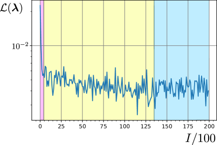
[Three phases of the training.]   [Implementations of the trainable variables.][width=8cm]variables_lambdas.svg

Figure 7: On the left picture the three phases of the learning process explained in Section E.1 are plotted. One tick on the $x$-axis corresponds to $500$ update steps. The agent first learns the rough form of the optimal strategy and later the fine details, before converging. On the right the three agents used in this work are represented, i.e a NN, a ternary decision tree, and a table containing the values of the controls $\boldsymbol{x}$, indexed by the measurement step $t$.

To end the section we briefly recap the three possible implementations that the trainable variables $\boldsymbol{\lambda}$ have taken in this work, see Fig. 7. In the case the agent is a NN $\boldsymbol{\lambda}$ are the weights and the biases of the network When the agent is a decision tree, the controls $x_{t}$ are associated to each node of the tree, and they are the $\boldsymbol{\lambda}$ variables. Finally, for a non-adaptive strategy, there is no adaptivity and the controls $\boldsymbol{x}$ are codified in a list, indexed by the measurement step $t$. In this case the controls and the training variables coincide, i.e. $\boldsymbol{\lambda}=\boldsymbol{x}_{M-1}$.

E.2 Fit of the precision

In this section we briefly comment on the way the precision plot are realized throughout the work. The definition of the resources doesn’t only impact the stopping condition of the measurement loop, but it defines how the performances of an agent are visualized, since by default we plot the mean loss as a function of the consumed resources. After having trained the agent we simulate many times the estimation and we keep track of the tuples $\mathcal{S}:=\{(R_{j},\mathcal{L}_{j})\}_{j=1}^{S}$ after each measurement step, containing the consumed resources $R_{t}$ and the loss $\mathcal{L}$. Since the experiment is a stochastic process we will collect a cloud of points from which a simple relation between the expected precision and the resources must be obtained, see Fig. 8.

[Clustering of the precision point cloud.][width=6cm]precision_average.svg   [Fit of the precision point cloud.][width=6cm]precision_nn.svg

Figure 8: On the left side we represent the precision plot where the cloud of points has been clustered to obtain the red crosses. On the right we use a NN to interpolate and get the average loss at a given value of the resources.

The first possibility is to divide the x-axis of the resources in intervals of size $\delta$, and compute the barycenters of all the points $(R_{j},\mathcal{L}_{j})$ falling in this interval, these would be the red crosses of Fig. 8. The second possibility is to fit this cloud of points with a NN. We set the training loss to be the MSE, i.e.

$$\mathcal{L}_{\text{fit}}:=\frac{1}{S}\sum_{j=1}^{S}\left[\mathcal{L}_{j}-f_{\text{NN}}(R_{j})\right]^{2}\;,$$ (123)

which, for a single value of the resource, i.e. $R_{j}=R\;\forall j$, would converge to $f_{\text{NN}}(R)=\frac{1}{S}\sum_{j=1}^{S}\mathcal{L}_{j}$, that is a NN will approximate the mean loss. This won’t be exactly true for a cloud of points, but with Eq. 123 we incentivise the NN to converge toward the average loss for every value of the resources. All the plots in this paper have been produced with the first method, choosing an appropriate $\delta$, except for those plots on the NV center platform with $T_{2}^{\star}=\infty$ and referring to the time-limited estimation. In the PGH line of the first plot in Fig. 2 there is a non-monotonicity for small $T$, that is a defect in the plot and an artifact on this way of interpolating with a NN.

E.3 Scaling of the time and memory requirements

Since the $B$ estimations in a batch can be performed in parallel we will benefit from the use of a GPU or a TPU (Tensor Processing Unit) in the training of the agent. The main difference between the CPU and the GPU is that a CPU has fewer ($\sim\mathcal{O}(10)$) faster cores, while a GPU has many ($\sim\mathcal{O}(10^{3})$) slower cores. With a large batchsize the use of hardware acceleration through a GPU will turn out to be essential and we will first examine the resource requirements of model-aware RL assuming that everything that can be parallelized has been is indeed executed in parallel. In this case the time requirement of the simulation is mainly influenced linearly by the number of measurements $M$ in the training loop, that have to be executed necessarily sequentially. The update of the PF and the computation of the distributions moments all require $\mathcal{O}(N)$ multiplications each but can be done in parallel, where $N$ is the number of particles. The memory requirement depends on the batchsize $B$ and the number of particles $N$ in the PF. Nevertheless because of the construction of the gradient, for which we need to keep in memory the results of all the intermediate computations, the number of measurements $M$ has also an almost linear influence on the required memory. Finally, the total time used in the training is also proportional to the number of update steps $I$. Each update step comprises the complete run of an estimation batch together with the evaluation of the gradient and the update of the controls. The size of the NN has little impact on the training time and memory. We can summarise the above considerations as

$$\text{Memory}\sim\mathcal{O}(BMN)\;,\quad\;\text{Time}_{\text{Par}}\sim\mathcal{O}(IM)\;.$$ (124)

Assuming that nothing can be parallelized (we have a single core) and therefore everything is sequential, if, as usual, the computational time in the CPU is dominated by the number of floating point multiplications, we instead have the time scaling

$$\text{Time}_{\text{Seq}}\sim\mathcal{O}(IBMN)\;,$$ (125)

while the memory requirement is unchanged. Neither a GPU nor a CPU will perfectly reproduce these theoretical scalings, because the GPU has a limited number of cores, but there is a tendency for a GPU to follow the scaling of $\text{Time}_{\text{Par}}$ and for a CPU $\text{Time}_{\text{Seq}}$. If the batchsize $B$ is very large (or the GPU not very powerful) the simulations in the batch can’t all be executed in parallel and $B$ starts to affect also the time requirements. If $B$ and $N$ are small a CPU may complete the training before a GPU, because of the smaller proportionality factor for the time requirement in Eq. 125 with respect to Eq. 124, due to the faster cores of the CPU. This analysis applies also to the training of a non-adaptive strategy, which is not resource-saving compared to the training of the NN. In the applications we expect our agent to run on a small controller near the sensor, where most definitely we won’t have access to a GPU and lots of memory, which anyway are required only in the training phase. In this situation we have no batch and only one iteration, i.e. $I=B=1$. Furthermore there is no extra $M$ in the memory requirement appearing because of the automatic differentiation, so that the resource scaling in the application will be

$$\text{Memory}\sim\mathcal{O}(dN+N)\;,\quad\;\text{Time}_{\text{Seq}}\sim\mathcal{O}(MN)\;,$$ (126)

where $d$ is the number of parameters. For an estimation limited by the resources instead of the number of measurements, $M$ must be intended as the average number of measurements employed for a fixed amount of resources. In general thanks to the resampling routine we can keep the number of particles fixed while increasing the precision arbitrarily. It is a good practise although to choose $N$ proportional to the number of parameters to estimate, i.e. $N\sim\mathcal{O}(d)$. In the applications the memory requirement of the NN, and the multiplications needed to evaluate it at each step contribute respectively with additional $\mathcal{O}(n_{l}n_{u})$ memory and $\mathcal{O}(n_{l}n_{u}^{2})$ time (per step), where $n_{l}$ is the number of layers and $n_{u}$ the number of units per layer, so that we have

$$\text{Memory}\sim\mathcal{O}(dN+N+n_{l}n_{u})\;,\quad\;\text{Time}_{\text{Seq}}\sim\mathcal{O}(MN+Mn_{l}n_{u}^{2})\;.$$ (127)

If the control is non-adaptive we don’t need this extra computations, and if the PF is removed from the picture (because we don’t need real time feedback) we have that the memory and time requirements trivialize, i.e they scale respectively as $\mathcal{O}(1)$ and $\mathcal{O}(M)$. Of course the total time of estimation would be influenced also by the time it takes to perform the physical measurement on the probe, but here we are referring only to the computational time.

Appendix F Optimal strategies for frequentist optimization

The qsensoropt library can also optimize the Cramér-Rao bound (based on the Fisher information matrix) for the local estimation of the parameters $\boldsymbol{\theta}$. This is frequentist inference instead of Bayesian inference, this last being the main topic of this work. The multiparameter Cramér-Rao bound (CR bound) is a lower bound on the Mean Square Error matrix of the frequentist estimator $\boldsymbol{\widehat{\theta}}$ at the position $\boldsymbol{\theta}$, expressed in terms of the FI matrix, i.e.

$$K:=\mathbb{E}\left[(\boldsymbol{\widehat{\theta}}-\boldsymbol{\theta})(\boldsymbol{\widehat{\theta}}-\boldsymbol{\theta})^{\intercal}\right]\geq F^{-1}(\boldsymbol{\theta})\;,$$ (128)

with

$$F_{ij}(\boldsymbol{\theta}):=\mathbb{E}_{y}\left[\frac{\partial\log p_{\boldsymbol{\theta}}(y)}{\partial\theta_{i}}\frac{\partial\log p_{\boldsymbol{\theta}}(y)}{\partial\theta_{j}}\right]\;.$$ (129)

This result sets the maximum achievable precision of an estimator around $\boldsymbol{\theta}$, in other words, it limits the ability to distinguish reliably two close values $\boldsymbol{\theta}$ and $\boldsymbol{\theta}+\delta\boldsymbol{\theta}$. The expectation value is taken on many realizations of the experiment, i.e. on the probability distribution of the trajectories for the outcomes and the controls. Let us introduce the tuple $\boldsymbol{x}$ and $\boldsymbol{y}$ containing respectively the entirety of the controls and the outcomes of the measurements done in the experiment, then the FI matrix has the following expression

$$F_{ij}(\boldsymbol{\theta}):=\mathbb{E}_{\boldsymbol{y}}\left[\frac{\partial\log p(\boldsymbol{y}|\boldsymbol{x},\boldsymbol{\theta})}{\partial\theta_{i}}\frac{\partial\log p(\boldsymbol{y}|\boldsymbol{x},\boldsymbol{\theta})}{\partial\theta_{j}}\right]\;,$$ (130)

being $p(\boldsymbol{y}|\boldsymbol{x},\boldsymbol{\theta})$ the probability of the observed trajectory of outcomes at the point $\boldsymbol{\theta}$. Notice that the expectation value is taken on the whole trajectory of the experiment. By contracting Eq. 128 with the weight matrix $G\geq 0$ we get the scalar version of the CR bound, i.e.

$$\text{tr}(G\cdot K)\geq\text{tr}(G\cdot F^{-1}):=\mathcal{L}(\boldsymbol{\lambda})\;,$$ (131)

where we have defined the loss to be optimized in the training, as a function of the trainable variables of the agent $\boldsymbol{\lambda}$. The gradient of the loss is

$$\frac{\partial\mathcal{L}}{\partial\boldsymbol{\lambda}}=\text{tr}\left(F^{-1}GF^{-1}\cdot\frac{\partial F}{\partial\boldsymbol{\lambda}}\right)\;.$$ (132)

The expectation value in the definition of $F$ is approximated in the simulation by averaging the product of the log-likelihoods derivatives on a batch of estimations, i.e.

$$F\simeq\widehat{F}=\frac{1}{B}\sum_{k=1}^{B}\frac{\partial\log p(\boldsymbol{y}_{k}|\boldsymbol{x}_{k},\boldsymbol{\theta})}{\partial\theta_{i}}\frac{\partial\log p(\boldsymbol{y}_{k}|\boldsymbol{x}_{k},\boldsymbol{\theta})}{\partial\theta_{j}}=\frac{1}{B}\sum_{k=1}^{B}f_{k}\;.$$ (133)

where $(\boldsymbol{x}_{k},\boldsymbol{y}_{k})$ is the trajectory of a particular realization of the experiment in the batch of simulations and $f_{k}$ is called the observed Fisher information. The unbiased gradient of the loss, that takes into account also the gradient of the probability distribution in the expectation value, can be computed as following

$$\frac{\partial\mathcal{L}}{\partial\boldsymbol{\lambda}}\simeq\frac{1}{B}\frac{\partial}{\partial\boldsymbol{\lambda}}\text{tr}\Big{\{}\text{sg}\left(\widehat{F}^{-1}G\widehat{F}^{-1}\right)\sum_{k=1}^{B}\left[f_{k}+\text{sg}(f_{k})\log p(\boldsymbol{x}_{k},\boldsymbol{y}_{k}|\boldsymbol{\theta})\right]\Big{\}}\;.$$ (134)

The $\text{sg}(\cdot)$ is the stop gradient operator, and the probability $p(\boldsymbol{x}_{k},\boldsymbol{y}_{k}|\boldsymbol{\theta})$ is the likelihood of the particular trajectory, that contains both the probability of the stochastic outcome and that of the control (in case it is stochastically generated). This is the gradient used in the update step of the stochastic gradient descent procedure for the optimization of frequentist estimation. We can also introduce the logarithmic loss, i.e.

$$\mathcal{L}_{\text{log}}(\boldsymbol{\lambda}):=\log\text{tr}(G\cdot F^{-1})\;,$$ (135)

which is particularly useful to stabilize the training when the FI spans multiple orders of magnitude. If we have a broad prior on $\boldsymbol{\theta}$, but we are stile interested in local estimation, we can introduce the average FI, i.e.

$$\mathcal{F}:=\int F(\boldsymbol{\theta})\pi(\boldsymbol{\theta})\mathop{\mathrm{d}\!}{}\boldsymbol{\theta}\;,$$ (136)

and optimize the loss

$$\mathcal{L}(\boldsymbol{\lambda}):=\text{tr}\left[G\cdot\mathcal{F}^{-1}\right]\leq\int\text{tr}\left[G\cdot F^{-1}(\boldsymbol{\theta})\right]\mathop{\mathrm{d}\!}{}\boldsymbol{\theta}\;,$$ (137)

which is a lower bound on the expectation value of the CR bound, because of the Jensen inequality applied to the matrix inverse. In the case of a single parameter the training would maximize the expected value of the Fisher information on the prior $\pi(\theta)$. It is possible to use a custom distribution $\widetilde{p}(y|x,\boldsymbol{\theta})$ for extracting the measurements outcomes instead of $p(y|x,\boldsymbol{\theta})$ by using importance sampling. In this case the FI matrix is computed as

$$F_{ij}(\boldsymbol{\theta})=\mathbb{E}_{\widetilde{p}}\left[\frac{\partial\log p(\boldsymbol{y}|\boldsymbol{x},\boldsymbol{\theta})}{\partial\theta_{i}}\frac{\partial\log p(\boldsymbol{y}|\boldsymbol{x},\boldsymbol{\theta})}{\partial\theta_{j}}\cdot\frac{p(\boldsymbol{y}|\boldsymbol{x},\boldsymbol{\theta})}{\widetilde{p}(\boldsymbol{y}|\boldsymbol{x},\boldsymbol{\theta},)}\right]\;,$$ (138)

which can be approximated on a batch as

$$F\simeq\frac{1}{B}\sum_{k=1}^{B}f_{k}\frac{p(\boldsymbol{y}_{k}|\boldsymbol{x}_{k},\boldsymbol{\theta})}{\widetilde{p}(\boldsymbol{y}_{k}|\boldsymbol{x}_{k},\boldsymbol{\theta})}\;,$$ (139)

with $f_{k}$ defined in Eq. 133. Also the gradient of $F$ is changed accordingly. Typically the distribution $\widetilde{p}$ is some perturbation of $p$, for example it can be obtained by mixing $p$ with a uniform distribution on the outcomes. The importance sampling is useful when some trajectories have vanishingly small probability of occurring according to the model $p$ but contribute significantly to the Fisher information. If these trajectories have some probability of occurring sampling with $\widetilde{p}$, then the estimator of the FI might be more accurate. The drawback is that the perturbed probability of the complete trajectory $\widetilde{p}(\boldsymbol{y}|\boldsymbol{x},\boldsymbol{\theta})$ might be too different from the real probability (because of the accumulation of the perturbation at each step), so that the simulation might entirely miss the region in the space of trajectories in which the system state moves, thus delivering a bad estimate of the FI and a bad control strategy, upon completion of the training. Whether or not the importance sampling can be beneficial to the optimization should be checked case by case. The derivative with respect to $\boldsymbol{\theta}$ in the definition of $f_{k}$ in Eq. 133 are computed through automatic differentiation. This means there there are two nested automatic differentiation environments, one for the parameter and one for the training variables of the agent.

Appendix G Precision lower bounds of the examples

In this section we apply the Bayesian Cramér-Rao bound to the estimation of various parameters on the NV center platform. This bounds will be based on the Fisher information [22], which we briefly define in the following. Refer to the literature for more details. Consider a stochastic variable $y$, which is extracted from a probability distribution $p_{\theta}(y)$, where $\theta$ is a parameter we want to estimate. This is a model for an experiment leading to a stochastic outcome. The information on $\theta$ available from $y$ can be measured by the Fisher information (FI), defined as

$$I(\theta):=\mathbb{E}_{y}\left[\left(\frac{\partial\log p_{\theta}(y)}{\partial\theta}\right)^{2}\right]\;,$$ (140)

where the expectation value is taken over the distribution $p_{\theta}(y)$. If the experiment allows to be controlled through the parameter $x$, then the outcome probability is $p_{\theta}(y|x)$ and the FI inherits such dependence, i.e. we write $I(\theta|x)$. If the control parameter $x$ is computed from a strategy $h$, which could be the Particle Guess Heuristic the a neural network, then we indicate it explicitly in the control $x_{h}$.

G.1 Bayesian Cramér-Rao bound

Given $\theta$ a single parameter to estimate, we call $I(\theta|\boldsymbol{x}_{h})$ the Fisher information of a sequence of measurements with controls $\boldsymbol{x}_{h}=(x_{0}^{h},x_{1}^{h},\cdots,x_{M-1}^{h})$, which are computed from a strategy $h$. The quantity $I(\theta|\boldsymbol{x}_{h})$, together with the Fisher information of the prior $\pi(\theta)$, i.e. $I(\pi)$, defines a lower bound on the precision $\Delta^{2}\widehat{\theta}$ of whatever estimator $\widehat{\theta}$, that contains the expectation value of $I(\theta|\boldsymbol{x}_{h})$ on $\pi(\theta)$, and is optimized on the strategy $h$. This lower bounds reads

$$\Delta^{2}\widehat{\theta}\geq\frac{1}{\sup_{h}\mathbb{E}_{\theta}\left[I(\theta|\boldsymbol{x}_{h})\right]+I(\pi)}\;.$$ (141)

This definition appears in the work of Fiderer et al. [32]. For the NV centers the controls are the evolution time $\tau$ and the phase $\varphi$, this last however doesn’t play any role in the computation of the lower bound, and it will be omitted in the following. The Fisher information of a sequence of measurements is always additive, even if the quantum probe is only measured weakly, but in dealing with projective measurements, as it is the case for NV center, the advantage is that the measurements are uncorrelated, and the same expression for the Fisher information applies to all of them, independently on the results of the previous measurements, i.e.

$$I(\theta|\boldsymbol{\tau})=\sum_{t=1}^{M}I(\theta|\tau_{t})\leq M\sup_{\tau}I(\theta|\tau)\;,$$ (142)

where $M$ is the total number of measurements. The optimization of the single measurement FI gives directly the precision bound for the measurement-limited estimation:

$$\Delta^{2}\widehat{\theta}\geq\frac{1}{\sup_{h}\mathbb{E}_{\theta}\left[I(\theta|\boldsymbol{\tau}_{h})\right]+I(\pi)}\geq\frac{1}{M\,\mathbb{E}_{\theta}\left[\sup_{\tau}I(\theta|\tau)\right]+I(\pi)}\;.$$ (143)

If the total evolution time is the limiting resource, then, the expression for the total FI is

$$I(\theta|\boldsymbol{\tau})=T\sum_{t=1}^{M}\frac{\tau_{t}}{T}\left[\frac{I(\theta|\tau_{t})}{\tau_{t}}\right]\leq T\sup_{\tau}\frac{I(\theta|\tau)}{\tau}\;,$$ (144)

with $\sum_{t=1}^{M}\tau_{t}=T$. In this expression the total FI is the weighted sum of the renormalized FI of each measurement, i.e. $\frac{I(\theta|\tau_{t})}{\tau_{t}}$, and can be manifestly upper bounded by concentrating all the weights on the supremum of the renormalized FI. This gives the lower bound for the precision of the time-limited estimation:

$$\Delta^{2}\widehat{\theta}\geq\frac{1}{\sup_{h}\mathbb{E}_{\theta}\left[I(\theta|\boldsymbol{\tau}_{h})\right]+I(\pi)}\geq\frac{1}{T\,\mathbb{E}_{\theta}\left[\sup_{\tau}\frac{I(\theta|\tau)}{\tau}\right]+I(\pi)}\;.$$ (145)

In the following we will apply this general observations to the derivation of the numerical bounds for DC magnetometry.

G.2 Evaluation of the Fisher information

Since the measurement outcome in the NV center is binary, we can compute the Fisher information for a parameter $\theta$, given the control $\tau$, as

$$I(\theta|\tau)=\mathbb{E}\left[\left(\frac{\partial\log p({\pm 1}|\theta,\tau)}{\partial\omega}\right)^{2}\right]=\frac{\left(\frac{\partial p}{\partial\theta}\right)^{2}}{p(1-p)}=\frac{\left(\frac{\partial p}{\partial\theta}\right)^{2}}{\frac{1}{4}-(p-\frac{1}{2})^{2}}\;,$$ (146)

where we have used the definition in Eq. 140, and where $p:=p(+1|\theta,\tau)$. For example, for a decoherence free estimation of the precession frequency $\omega$ we have $p:=\cos^{2}\left(\frac{\omega\tau}{2}\right)$, from which $\frac{\partial p}{\partial\theta}=\tau\sin(\frac{\omega\tau}{2})\cos(\frac{\omega\tau}{2})$, and finally $I(\omega|\tau)=\tau^{2}$.

G.3 DC magnetometry

The lower bounds on the estimation of the frequency $\omega$ are reported in Table 1, and are represented in Fig. 2 of Section II as the shaded grey area. The left column of this table contains the bounds for a finite number of measurements $M$, while right column refers to the estimation with a fixed total evolution time $T$. The first row refers to the estimation of $\omega$ with perfect coherence while the second row refers to the estimation of $\omega$ with a finite and know $T_{2}^{\star}$. The symbol $I(\omega)$ indicate the FI of the prior for the precession frequency $\omega$.

	Measurement		Time
$T_{2}=\infty$	$\frac{2^{-2(M+1)}}{3}$	147	$\frac{1}{T^{2}+I(\omega)}$	148
$T_{2}<\infty$	$\max\Big{\{}\frac{1}{\mu M(T_{2}^{\star})^{2}+I(\omega)},\frac{2^{-2(M+1)}}{3}\Big{\}}$	149	$\frac{1}{0.5\,TT_{2}^{\star}+I(\omega)}$	150

Table 1: Lower bounds for the precision of the frequency estimation in DC magnetometry on an NV center.

The numerical values of the quantities appearing in Table 1, for $\omega\in(0,1)\,\text{MHz}$ are: $\mu=0.1619$, $I(\omega)=12\,\mu\text{s}^{2}$. In the following we derive these four bounds.

• The Fisher information for the decoherence-free precession frequency $\omega$ is given by $I(\omega|\tau)=\tau^{2}$, so that $\sup_{\tau}I(\omega|\tau)=\infty$ and the analysis based on the Cramèr-Rao bound doesn’t gives a useful bound. Table 1 can be found by observing that each measurement gives at most one bit of information about the value of $\omega$, because the measurement has a binary outcomes [32]. This bound is applied also for $T_{2}^{\star}<\infty$ in addiction to the one coming from the Fisher information.

• With a finite decoherence time $T_{2}^{\star}<\infty$ the FI for the frequency $\omega$ is

  $$I(\omega|\tau,T_{2}^{\star})=\frac{\tau^{2}e^{-\frac{2\tau}{T_{2}^{\star}}}\cos^{2}\left(\frac{\omega\tau}{2}\right)\sin^{2}\left(\frac{\omega\tau}{2}\right)}{\left[e^{-\frac{\tau}{T_{2}^{\star}}}\cos^{2}\left(\frac{\omega\tau}{2}\right)+\frac{1-e^{-\frac{\tau}{T_{2}^{\star}}}}{2}\right]\left[e^{-\frac{\tau}{T_{2}^{\star}}}\sin^{2}\left(\frac{\omega\tau}{2}\right)+\frac{1-e^{-\frac{\tau}{T_{2}^{\star}}}}{2}\right]}\;,$$ (151)

  which, by defining $C:=\cos^{2}\left(\frac{\omega\tau}{2}\right)$, can be bounded in the following way

  $$I(\omega|\tau,T_{2}^{\star})=\frac{\tau^{2}e^{-\frac{2\tau}{T_{2}^{\star}}}C(1-C)}{\left[\frac{1}{4}-e^{-\frac{2\tau}{T_{2}^{\star}}}(C-\frac{1}{2})^{2}\right]}\leq\frac{\tau^{2}e^{-\frac{2\tau}{T_{2}^{\star}}}}{1-e^{-\frac{2\tau}{T_{2}^{\star}}}}=(T_{2}^{\star})^{2}\frac{x^{2}e^{-2x}}{1-e^{-2x}}\;,$$ (152)

  where $x=\frac{\tau}{T_{2}^{\star}}$. The maximization in $x\in\mathbb{R}_{+}$ gives $\sup_{\tau}I(\omega|\tau,T_{2}^{\star})=\mu(T_{2}^{\star})^{2}$ with $\mu=0.1619$. Inserting this expression in Eq. 143 gives the first term in the maximum of Table 1, the second term was explained in the previous point.

• Regarding the time-constrained lower bounds, for $T_{2}^{\star}=\infty$, the total FI is maximized by performing a single measurement of time duration $\tau=T$, which gives Table 1, through the application of Eq. 145.

• For $T_{2}^{\star}<\infty$ we have to maximize the normalized FI in $x\in\mathbb{R}_{+}$, i.e.

  $$\frac{I(\omega|\tau,T_{2}^{\star})}{\tau}\leq\frac{\tau e^{-\frac{2\tau}{T_{2}^{\star}}}}{1-e^{-\frac{2\tau}{T_{2}^{\star}}}}\leq T_{2}^{\star}\frac{xe^{-2x}}{1-e^{-2x}}\leq\frac{TT_{2}^{\star}}{2}\;,$$ (153)

  from which Table 1 follows from Eq. 145.

Appendix H Backward recursion method for the optimization of the strategy

In this section we set the stage to understand what function the agent must approximate by formulating the problem in terms of a backward recursion. In this section we will see how the optimal control could theoretically be derived in other ways, so that the training will appear less as an unintelligible black-box and more as the solution to a well-posed problem (though we won’t probably have uniqueness). The output of the agent at the $t+1$-th steps is $x_{t+1}$, that is, the control of the current evolutions and measurements. In the following we will define formally the function that the agent must learn to approximate, in doing this we will assume that the control $x$ of the quantum sensor is a continuos real variable. Consider an estimation with $M$ measurements, i.e. $t=0,1,\dots,M-1$. Let us focus on the last one only and recall the definition of the particle filter ensemble before after the last measure $M-1$, i.e. $\mathfrak{p}_{M}:=\{\boldsymbol{\theta}^{M-1}_{j},w^{M-1}_{j}\}_{j=1}^{N}$. Then we can write the ensemble of the PF at the final step $t=M-1$ as

$$\mathfrak{p}_{M}=\mathfrak{B}(\mathfrak{p}_{M-1},x_{M-1},y_{M-1})\;,$$ (154)

where $\mathfrak{B}$ encodes the application of the Bayes rule in Eq. 20. The ensemble $\mathfrak{p}_{M}$ inherits the stochasticity from the random measurement outcome $y_{M-1}$. Per definition $\mathfrak{p}_{0}$ is the initial PF ensemble that represents the prior $\pi(\boldsymbol{\theta})$. In Section D.1 we mentioned that the final loss is a scalar function $\ell(\mathfrak{p}_{M},\boldsymbol{\theta})$ of the final PF ensemble and of the true value $\boldsymbol{\theta}$, like the squared derivation of the estimator from the true value. The final loss can be expressed as $\ell(\mathfrak{B}(\mathfrak{p}_{M-1},x_{M-1},y_{M-1}),\boldsymbol{\theta})$ and it’s expectation value on $y_{M-1}$ (the expected loss), computed with the density in Eq. 15, reads

$$\overline{\ell}(\mathfrak{p}_{M-1},x_{M-1},\boldsymbol{\theta}):=\int\ell(\mathfrak{B}(\mathfrak{p}_{M-1},x_{M-1},y_{M-1}),\boldsymbol{\theta})p(y_{M-1}|x_{M-1},\boldsymbol{\theta})dy_{M-1}\;.$$ (155)

If the outcome probability, the prior and the loss are continuos functions we can also expect $\overline{\ell}(\mathfrak{p}_{M-1},x_{M-1},\boldsymbol{\theta})$ to be continuous in its parameters. Without aiming at full rigour, we say that the regularity properties of the probability densities are passed down to the expectation value. Now we look for the minimum of this function, which is realized by solving

$$\frac{\mathop{\mathrm{d}\!}{}\overline{\ell}(\mathfrak{p}_{M-1},x_{M-1}^{\star},\boldsymbol{\theta})}{\mathop{\mathrm{d}\!}{}x_{M-1}}=0\;.$$ (156)

This equation defines implicitly the optimal control $x_{M-1}^{\star}:=r_{M-1}(\mathfrak{p}_{M-1},\boldsymbol{\theta})$, where $x_{M-1}^{\star}$ realizes the absolute minimum of the expected loss. $r_{M-1}$ inherits some regularity property (at least locally) from $\overline{\ell}(\mathfrak{p}_{M-1},x_{M-1},\boldsymbol{\theta})$ thanks to the implicit function theorem. The control $x_{M-1}^{\star}$ can still have discontinuities in $\mathfrak{p}_{M-1}$ if the expected loss has multiple competing minima. The dependence on $\boldsymbol{\theta}$ is rather inconvenient, because it is unknown, but we can think of substituting $\boldsymbol{\theta}$ with its estimator $\boldsymbol{\widehat{\theta}}_{M-2}$ to get $x_{M-1}^{\star}=r_{M-1}(\mathfrak{p}_{M-1},\boldsymbol{\widehat{\theta}}_{M-2})$. We will however never do explicit optimizations with this approach, the introduction of Machine Learning in quantum metrology serves precisely to avoid these cumbersome computations. Until now we have only optimized the last control, but fortunately all these operations can be repeated with minor changes for the $t=M-2$ measurement step. Let us start from $\mathfrak{p}_{M-1}$ expressed as function of the ensemble $\mathfrak{p}_{M-2}$:

$$\mathfrak{p}_{M-1}=\mathfrak{B}(\mathfrak{p}_{M-2},x_{M-2},y_{M-2})\;,$$ (157)

we insert this expression in Eq. 154 to get

$$\mathfrak{p}_{M}=\mathfrak{B}(\mathfrak{B}(\mathfrak{p}_{M-2},x_{M-2},y_{M-2}),x_{M-1},y_{M-1})\;.$$ (158)

By substituting this in the loss $\ell(\mathfrak{p}_{M},\boldsymbol{\theta})$ we get $\ell(\mathfrak{B}(\mathfrak{B}(\mathfrak{p}_{M-2},x_{M-2},y_{M-2}),x_{M-1},y_{M-1}),\boldsymbol{\theta})$, but the optimal $x_{M-1}$ has been already computed as a function of the PF ensemble. Whatever control we suggest for the step $t=M-2$ it doesn’t change the optimal control at the following step. In other words whatever control $x_{M-2}$ gets applied, the optimal action for the last time step is always $x_{M-1}^{\star}$, we can therefore insert it in the loss at the step $M-2$, i.e.

$$\ell(\mathfrak{p}_{M-2},x_{M-2},y_{M-2},y_{M-1},\boldsymbol{\theta}):=\ell(\mathfrak{B}(\mathfrak{B}(\mathfrak{p}_{M-2},x_{M-2},y_{M-2}),r_{M-1}(\mathfrak{B}(\mathfrak{p}_{M-2},x_{M-2},y_{M-2}),\boldsymbol{\theta}),y_{M-1}),\boldsymbol{\theta})\;,$$ (159)

where we have also used the expression for $\mathfrak{p}_{M-1}$ of Eq. 157 in the definition of $x_{M-1}^{\star}$, and we have redefined the parameters of $\ell$. Again we take the expectation value on the measurement outcomes, i.e.

$$\overline{\ell}(\mathfrak{p}_{M-2},x_{M-2},\boldsymbol{\theta}):=\int\ell(\mathfrak{p}_{M-2},x_{M-2},y_{M-2},y_{M-1},\boldsymbol{\theta})p(y_{M-1}|\boldsymbol{\theta},x_{M-1}^{\star})p(y_{M-2}|\boldsymbol{\theta},x_{M-2})dy_{M-1}dy_{M-2}\;.$$ (160)

By taking the derivative of this expected loss with respect to $x_{M-2}$, we define implicitly the optimal control $x_{M-2}^{\star}=r_{M-2}(\mathfrak{p}_{M-2},\boldsymbol{\theta})$ as the solution of

$$\frac{\mathop{\mathrm{d}\!}{}\overline{\ell}(\mathfrak{p}_{M-2},x_{M-2}^{\star},\boldsymbol{\theta})}{\mathop{\mathrm{d}\!}{}x_{M-2}}=0\;,$$ (161)

where $x_{M-2}^{\star}$ realizes the absolute minimum of $\overline{\ell}$. Notice that this is not a greedy optimization: the value of $x_{M-2}$ is not chosen to optimize the loss one step head in the future but the final loss, knowing what the strategy in the next step will be. We could treat all the previous measurements in the same manner, if it wasn’t for the expectation values of the loss, that become more and more complicated. In this way we can inductively proceed in reverse to the start of the estimation $t=0$ and find in the process the family of functions $r_{t}(\mathfrak{p}_{t},\boldsymbol{\theta}_{t-1})$ that express the optimal controls $x_{t}^{\star}$. As discussed previously we can redefine $r_{t}(\mathfrak{p}_{t})=r_{t}(\mathfrak{p}_{t},\boldsymbol{\widehat{\theta}}_{t-1})$, in order to get rid of the dependence on the unknown value of the parameters $\boldsymbol{\theta}$. We then introduce $r(\mathfrak{p}_{t},t)=r_{t}(\mathfrak{p}_{t})$, which is the function that the agent is trying to approximate in the training, i.e. the map that spits out the optimal control at a given measurement step $t$, provided the ensemble PF at the previous step. Heuristically we expect the optimal control to be inhomogeneous in time because like in many application of RL a good strategy encompasses a phase of “exploration” followed by a phase of “exploitation” of what has been learned [18, 19].

Appendix I Backpropagation of the gradient

With the help of an automatic differentiation framework we compute the gradient of the modified loss in Eq. 92 in order to perform the training. Let us for the moment neglect the log-likelihood terms in this expression and concentrate only on the first part. If the loss is computed only from the ensemble at the last measurement step, then it takes the form

$$\ell_{\boldsymbol{\theta}}\circ\mathfrak{B}_{x_{M-1},y_{M-1}}\circ\mathfrak{B}_{x_{M-1},y_{M-1}}\circ\cdots\circ\mathfrak{B}_{x_{0},y_{0}}(\mathfrak{p}_{0})\;.$$ (162)

where $\ell_{\boldsymbol{\theta}}(\mathfrak{p}):=\ell(\mathfrak{p},\boldsymbol{\theta})$ acts on the ensemble PF and is the individual loss of each simulation, e.g. the square error. The function $\mathfrak{B}_{x_{t},y_{t}}(\mathfrak{p}):=\mathfrak{B}(\mathfrak{p},x_{t},y_{t})$ applies the Bayesian update to the PF, which depends on the outcome of the measurement $y_{t}$ and on the control $x_{t}$. The initial ensemble of the PF is named $\mathfrak{p}_{0}$. From a theoretical point of view differentiating this expression means applying repeatedly the rule for the derivation of the composite function and propagating the derivative through the various stages of the estimation, this is called backpropagation. Let us compute explicitly the derivative of the loss for the last two steps of the estimation. We define $\mathfrak{p}_{M}=\mathfrak{B}_{x_{M-1},y_{M-1}}(\mathfrak{p}_{M-1})$ and $\mathfrak{p}_{M-1}=\mathfrak{B}_{x_{M-2},y_{M-2}}(\mathfrak{p}_{M-2})$, and apply the chain rule. We will indicate with the partial derivative symbol the derivatives with respect to the parameters of a function (which can also appear in the subscript), while the symbol $\frac{\mathop{\mathrm{d}\!}{}}{\mathop{\mathrm{d}\!}{}\boldsymbol{\lambda}}$ is reserved to the total derivative with respect to $\boldsymbol{\lambda}$.

$$\frac{\mathop{\mathrm{d}\!}{}}{\mathop{\mathrm{d}\!}{}\boldsymbol{\lambda}}\ell_{\boldsymbol{\theta}}(\mathfrak{p}_{M})=\frac{\partial\ell_{\boldsymbol{\theta}}(\mathfrak{p}_{M})}{\partial\mathfrak{p}}\frac{\mathop{\mathrm{d}\!}{}}{\mathop{\mathrm{d}\!}{}\boldsymbol{\lambda}}\mathfrak{B}_{x_{M-1},y_{M-1}}(\mathfrak{p}_{M-1})\;.$$ (163)

The total derivate in the right-hand term an be expanded again with the chain rule:

$$\frac{\partial\mathfrak{B}_{x_{M-1},y_{M-1}}(\mathfrak{p}_{M-1})}{\partial x_{M-1}}\frac{\mathop{\mathrm{d}\!}{}}{\mathop{\mathrm{d}\!}{}\boldsymbol{\lambda}}x_{M-1}(\boldsymbol{\lambda},\mathfrak{p}_{M-1})+\color[rgb]{1,0,0}\underline{{\color[rgb]{0,0,0}\frac{\partial\mathfrak{B}_{x_{M-1},y_{M-1}}(\mathfrak{p}_{M-1})}{\partial\mathfrak{p}}\frac{\mathop{\mathrm{d}\!}{}}{\mathop{\mathrm{d}\!}{}\boldsymbol{\lambda}}\mathfrak{B}_{x_{M-2},y_{M-2}}(\mathfrak{p}_{M-2})}}\color[rgb]{0,0,0}\quad\text{a)}\;.$$ (164)

Only the parameters $x_{M-1}$ and $\mathfrak{p}_{M-1}$ can carry a dependence on $\boldsymbol{\lambda}$. Regarding the measurement outcomes $y_{M-1}$ we already discussed their independence on $\boldsymbol{\lambda}$, expressed by Eq. 84. The control $x_{M-1}$ has an explicit dependence on $\boldsymbol{\lambda}$ because it has been produced by the agents, but also has a dependence on $\boldsymbol{\lambda}$ through the PF ensemble, so that we can expand the total derivative in the following way

$$\frac{\mathop{\mathrm{d}\!}{}}{\mathop{\mathrm{d}\!}{}\boldsymbol{\lambda}}x_{M-1}(\boldsymbol{\lambda},\mathfrak{p}_{M-1}) =\color[rgb]{0,0,1}\underline{{\color[rgb]{0,0,0}\frac{\partial x_{M-1}(\boldsymbol{\lambda},\mathfrak{p}_{M-1})}{\partial\boldsymbol{\lambda}}}}\color[rgb]{0,0,0}\quad\text{b)}$$ (165)

$$+\color[rgb]{0,1,0}\underline{{\color[rgb]{0,0,0}\frac{\partial x_{M-1}(\boldsymbol{\lambda},\mathfrak{p}_{M-1})}{\partial\mathfrak{p}}\frac{\mathop{\mathrm{d}\!}{}}{\mathop{\mathrm{d}\!}{}\boldsymbol{\lambda}}\mathfrak{B}_{x_{M-2},y_{M-2}}(\mathfrak{p}_{M-2})}}\color[rgb]{0,0,0}\quad\text{c)}\;.$$ (166)

The first piece of the derivative is the dependence on $\boldsymbol{\lambda}$ that comes from the last application of the agent, while the second piece represent the backpropagation through the input of the agent and the Bayesian update of the PF ensemble. In general, the gradient is backpropagated through all the applications of the agent until it reaches the beginning. We notice that we can write the total derivative of $\mathfrak{p}_{M}$ as a function of the total derivative of $\mathfrak{p}_{M-1}$, i.e.

$$\frac{\mathop{\mathrm{d}\!}{}}{\mathop{\mathrm{d}\!}{}\boldsymbol{\lambda}}\mathfrak{B}_{x_{M-1},y_{M-1}}(\mathfrak{p}_{M-1})=Q_{M-1}+H_{M-1}\frac{\mathop{\mathrm{d}\!}{}}{\mathop{\mathrm{d}\!}{}\boldsymbol{\lambda}}\mathfrak{B}_{x_{M-2},y_{M-2}}(\mathfrak{p}_{M-2})$$ (167)

where

$$Q_{M-1} := \frac{\partial\mathfrak{B}_{x_{M-1},y_{M-1}}(\mathfrak{p}_{M-1})}{\partial x_{M-1}}\frac{\partial x_{M-1}(\boldsymbol{\lambda},\mathfrak{p}_{M-1})}{\partial\boldsymbol{\lambda}}\;,$$ (168)

$$H_{M-1} := \frac{\partial\mathfrak{B}_{x_{M-1},y_{M-1}}(\mathfrak{p}_{M-1})}{\partial x_{M-1}}\frac{\partial x_{M-1}(\boldsymbol{\lambda},\mathfrak{p}_{M-1})}{\partial\mathfrak{p}}+\frac{\partial\mathfrak{B}_{x_{M-1},y_{M-1}}(\mathfrak{p}_{M-1})}{\partial\mathfrak{p}}\;.$$ (169)

We have arrived to a family of recurrence equations, which have the solution

$$\frac{\mathop{\mathrm{d}\!}{}}{\mathop{\mathrm{d}\!}{}\boldsymbol{\lambda}}\mathfrak{B}_{x_{M-1},y_{M-1}}(\mathfrak{p}_{M-1})=\sum_{t=0}^{M-1}Q_{t}\prod_{m=t+1}^{M-1}H_{m}\;,$$ (170)

where $Q_{t}$ and $H_{m}$ are defined analogously to $Q_{M-1}$ and $H_{M-1}$. The $H_{m}$ terms have each two summand, and when multiplied together the number of terms in the gradient grows exponentially in the number of measurement $M$, and generates gradient terms corresponding to multiple repeated backpropagations through the agents. This are a kind of “higher order” gradient terms. In our implementation of the training we simplify the gradient by introducing a stop gradient operation before the input of the agent, so that Eq. 2 is actually implemented as

$$x_{t+1}=\mathcal{F}\{\text{sg}\left[P(\boldsymbol{\theta}|\boldsymbol{x}_{t},\boldsymbol{y}_{t});R_{t};t\right]\}\;,$$ (171)

This modification doesn’t change the forward pass, that is, the results of simulations are the same, but it affects the backpropagation of the gradient, in particular it makes the first term of $H_{m}$ disappear, because

$$\frac{\partial x_{m}\left(\boldsymbol{\lambda},\text{sg}\left[\mathfrak{p}_{m}\right]\right)}{\partial\mathfrak{p}}=0\;.$$ (172)

Such simplification reduces considerably the training time and doesn’t really affect, at least from a theoretical point of view, the ability of the agent to learn the optimal strategy, on the contrary it might even improve it. Before we back up this last assertions we want to recapitulate our analysis of the backpropagation with the help of Fig. 9.

[width=0.8]gradient_flow.svg

Figure 9: The fat empty arrow in the middle of the picture represents the PF, which is updated via the Bayes rule, indicated with the function $\mathfrak{B}$ in the text, after it receive an outcome from the measurement on the probe. The second term of Eq. 164, underlined in red and labelled with a), corresponds to the backpropagation of the gradient along the history of the PF ensemble, whose weights and particles inherits a dependence on $\boldsymbol{\lambda}$ from the actions of the agent. Visually this corresponds to backpropagation along the red arrow labelled with a). Through the match between the underlined terms in Eq. 166 and Eq. 164 and the arrows in the figure can visualize the origin of each term of the gradient. The blue term of Eq. 166 labelled with b) accounts for the dependence on $\boldsymbol{\lambda}$ that comes from the controls computed by the agent and propagated through the application of the Bayes rule and the computation of $x_{t}$. The green term of Eq. 166 labelled with c) is the gradient propagating from the input of the agent to the previous PF ensemble. This term is responsible for the “higher-order” terms of the gradient, that propagate multiple times through the agent. Inserting the stop gradient in Eq. 172 means cutting the green line. The dashed yellow line represents the propagation of the gradient through the state of the probe, when this is not reinitialized between the measurements.

A control strategy is called myopic if it optimizes the information gained from the next measurement only, while it is non-myopic if it optimizes many steps ahead in the future. It might seem that by cutting the gradient propagation through the green arrows we limit the optimization to the class of myopic strategies, but this is not true because the optimization is always done for the final precision. The input of the agent is basically a constant now and the $t$-th term in the summation of Eq. 170 pulls the weights of the NN to minimize the final loss given the PF ensemble at the $t-1$-th step. In order to have non-myopic adaptive strategy backpropagating the gradient through the green arrows is redundant. The gradient of the log-likelihood terms in the loss of Eq. 93 is also simplified when the stop gradient is acting in Eq. 172. In the model $p(y_{t}|x_{t},\boldsymbol{\theta})$ the only term that depends on $\boldsymbol{\lambda}$ is the control, and the gradient propagates through a single application of the agent. Had we not inserted the stop gradient, the gradient of each summands in the log-likelihood would have been propagated through all the past applications of the agent, a scenario that happens anyway if the probe state is not reinitialized between measurements. Before ending the discussion on the gradient backpropagation we want to consider yet another possibility of truncating the gradient. We could indeed image to stop the flow of the derivative through the evolution of the PF ensemble, which means cutting the red line in Eq. 164. This eliminates the recurrence equation and trivializes the gradient, which now accounts only for the very last control. That is, with such modification, the agent will learn to optimize only the last measurement. If the loss is cumulative however, like in Eq. 106, all the controls will be optimized, but in a myopic way. In this scenario we introduce the modified logarithmic loss, i.e.

$$\widetilde{\mathcal{L}}_{\text{log}}(\boldsymbol{\lambda}):=\frac{1}{TB}\sum_{t=1}^{M-1}\log\left[\frac{\sum_{k=1}^{B}\ell(\boldsymbol{\widehat{\theta}}_{k,t},\boldsymbol{\theta}_{k})}{\text{sg}\left[\sum_{k=1}^{B}\ell(\boldsymbol{\widehat{\theta}}_{t-1,k},\boldsymbol{\theta}_{k})\right]}\right]\;.$$ (173)

Each term in this summation is the empirical information gain for a Gaussian posterior. In the forward pass the loss is the total empirical information gain, because the stop gradient operators don’t play any role, and the series can be resummed. In the computation of the gradient, however, the information gain for each measurement is optimized greedily, as done in [73] and in the package optbayesexpt [41]. If the stop gradient in the denominator is applied only every $n$ measurement, then we are optimizing the information gain planning $n$ steps ahead in the future. It is advisable to put a regularization at the denominator of the loss in Eq. 173 to avoid dividing by zero.

References

- [1] Flamini, F. et al. Photonic architecture for reinforcement learning. New Journal of Physics 22, 045002 (2020). URL https://iopscience.iop.org/article/10.1088/1367-2630/ab783c.
- [2] Broughton, M. et al. TensorFlow Quantum: A Software Framework for Quantum Machine Learning (2021). URL http://arxiv.org/abs/2003.02989.
- [3] Bergholm, V. et al. PennyLane: Automatic differentiation of hybrid quantum-classical computations (2022). URL http://arxiv.org/abs/1811.04968.
- [4] Bukov, M. et al. Reinforcement Learning in Different Phases of Quantum Control. Physical Review X 8, 031086 (2018). URL https://link.aps.org/doi/10.1103/PhysRevX.8.031086.
- [5] Zhang, X.-M., Wei, Z., Asad, R., Yang, X.-C. & Wang, X. When does reinforcement learning stand out in quantum control? A comparative study on state preparation. npj Quantum Information 5, 85 (2019). URL http://www.nature.com/articles/s41534-019-0201-8.
- [6] Niu, M. Y., Boixo, S., Smelyanskiy, V. N. & Neven, H. Universal quantum control through deep reinforcement learning. npj Quantum Information 5, 33 (2019). URL http://www.nature.com/articles/s41534-019-0141-3.
- [7] Porotti, R., Essig, A., Huard, B. & Marquardt, F. Deep Reinforcement Learning for Quantum State Preparation with Weak Nonlinear Measurements. Quantum 6, 747 (2022). URL https://quantum-journal.org/papers/q-2022-06-28-747/.
- [8] Porotti, R., Peano, V. & Marquardt, F. Gradient-Ascent Pulse Engineering with Feedback. PRX Quantum 4, 030305 (2023). URL https://link.aps.org/doi/10.1103/PRXQuantum.4.030305.
- [9] Fösel, T., Tighineanu, P., Weiss, T. & Marquardt, F. Reinforcement Learning with Neural Networks for Quantum Feedback. Physical Review X 8, 031084 (2018). URL https://link.aps.org/doi/10.1103/PhysRevX.8.031084.
- [10] Cimini, V. et al. Calibration of Quantum Sensors by Neural Networks. Physical Review Letters 123, 230502 (2019). URL https://link.aps.org/doi/10.1103/PhysRevLett.123.230502.
- [11] Ban, Y., Echanobe, J., Ding, Y., Puebla, R. & Casanova, J. Neural-network-based parameter estimation for quantum detection. Quantum Science and Technology 6, 045012 (2021). URL https://iopscience.iop.org/article/10.1088/2058-9565/ac16ed.
- [12] Nolan, S., Smerzi, A. & Pezzè, L. A machine learning approach to Bayesian parameter estimation. npj Quantum Information 7, 169 (2021). URL https://www.nature.com/articles/s41534-021-00497-w.
- [13] Nolan, S. P., Pezzè, L. & Smerzi, A. Frequentist parameter estimation with supervised learning. AVS Quantum Science 3, 034401 (2021). URL https://avs.scitation.org/doi/10.1116/5.0058163.
- [14] Nguyen, V. et al. Deep reinforcement learning for efficient measurement of quantum devices. npj Quantum Information 7, 100 (2021). URL http://www.nature.com/articles/s41534-021-00434-x.
- [15] Palmieri, A. M. et al. Experimental neural network enhanced quantum tomography. npj Quantum Information 6, 20 (2020). URL http://www.nature.com/articles/s41534-020-0248-6.
- [16] Quek, Y., Fort, S. & Ng, H. K. Adaptive quantum state tomography with neural networks. npj Quantum Information 7, 105 (2021). URL http://www.nature.com/articles/s41534-021-00436-9.
- [17] Hsieh, H.-Y. et al. Direct Parameter Estimations from Machine Learning-Enhanced Quantum State Tomography. Symmetry 14, 874 (2022). URL https://www.mdpi.com/2073-8994/14/5/874.
- [18] Marquardt, F. Machine learning and quantum devices. SciPost Physics Lecture Notes 29 (2021). URL https://scipost.org/10.21468/SciPostPhysLectNotes.29.
- [19] Marquardt, F. Online Course: Advanced Machine Learning for Physics, Science, and Artificial Scientific Discovery (2021).
- [20] Krenn, M., Landgraf, J., Foesel, T. & Marquardt, F. Artificial intelligence and machine learning for quantum technologies. Physical Review A 107, 010101 (2023). URL https://link.aps.org/doi/10.1103/PhysRevA.107.010101.
- [21] Belliardo, F., Zoratti, F. & Giovannetti, V. Application of machine learning to experimental design in quantum mechanics URL https://www.worldscientific.com/doi/abs/10.1142/S0219749924500023.
- [22] Fisher, R. A. The design of experiments. The design of experiments (Oliver & Boyd, Oxford, England, 1935).
- [23] Foster, A. E. Variational, Monte Carlo and policy-based approaches to Bayesian experimental design. http://purl.org/dc/dcmitype/Text, University of Oxford (2021). URL https://ora.ox.ac.uk/objects/uuid:4a3e13ca-e6c6-4669-955e-f1a87e201228.
- [24] Baydin, A. G. et al. Toward Machine Learning Optimization of Experimental Design. Nuclear Physics News 31, 25–28 (2021). URL https://www.tandfonline.com/doi/full/10.1080/10619127.2021.1881364.
- [25] Ballard, Z., Brown, C., Madni, A. M. & Ozcan, A. Machine learning and computation-enabled intelligent sensor design. Nature Machine Intelligence 3, 556–565 (2021). URL http://www.nature.com/articles/s42256-021-00360-9.
- [26] Ivanova, D. R., Foster, A., Kleinegesse, S., Gutmann, M. U. & Rainforth, T. Implicit Deep Adaptive Design: Policy-Based Experimental Design without Likelihoods. In Advances in Neural Information Processing Systems, vol. 34, 25785–25798 (Curran Associates, Inc., 2021). URL https://proceedings.neurips.cc/paper/2021/hash/d811406316b669ad3d370d78b51b1d2e-Abstract.html.
- [27] Sarra, L. & Marquardt, F. Deep Bayesian Experimental Design for Quantum Many-Body Systems (2023). URL http://arxiv.org/abs/2306.14510.
- [28] Foster, A., Ivanova, D. R., Malik, I. & Rainforth, T. Deep Adaptive Design: Amortizing Sequential Bayesian Experimental Design. In Proceedings of the 38th International Conference on Machine Learning, 3384–3395 (PMLR, 2021). URL https://proceedings.mlr.press/v139/foster21a.html.
- [29] Ścibior, A. & Wood, F. Differentiable Particle Filtering without Modifying the Forward Pass (2021). URL http://arxiv.org/abs/2106.10314.
- [30] Chen, M. et al. Quantum metrology with single spins in diamond under ambient conditions. National Science Review 5, 346–355 (2018). URL https://academic.oup.com/nsr/article/5/3/346/4430770.
- [31] Rembold, P. et al. Introduction to quantum optimal control for quantum sensing with nitrogen-vacancy centers in diamond. AVS Quantum Science 2, 024701 (2020). URL http://avs.scitation.org/doi/10.1116/5.0006785.
- [32] Fiderer, L. J., Schuff, J. & Braun, D. Neural-Network Heuristics for Adaptive Bayesian Quantum Estimation. PRX Quantum 2, 020303 (2021). URL https://link.aps.org/doi/10.1103/PRXQuantum.2.020303.
- [33] Arshad, M. J. et al. Online adaptive estimation of decoherence timescales for a single qubit (2022). URL http://arxiv.org/abs/2210.06103.
- [34] Joas, T. Online adaptive quantum characterization of a nuclear spin. npj Quantum Information 8 (2021).
- [35] Zoratti, F., Pozza, N. D., Fanizza, M. & Giovannetti, V. An agnostic-Dolinar receiver for coherent states classification. Physical Review A 104, 042606 (2021). URL http://arxiv.org/abs/2106.11909.
- [36] Fallani, A., Rossi, M. A. C., Tamascelli, D. & Genoni, M. G. Learning Feedback Control Strategies for Quantum Metrology. PRX Quantum 3, 020310 (2022). URL https://link.aps.org/doi/10.1103/PRXQuantum.3.020310.
- [37] Belliardo, F., Zoratti, F., Marquardt, F. & Giovannetti, V. In preparation: The qsensoropt library: examples and applications .
- [38] Meyer, J. J., Borregaard, J. & Eisert, J. A variational toolbox for quantum multi-parameter estimation. npj Quantum Information 7, 1–5 (2021). URL https://www.nature.com/articles/s41534-021-00425-y.
- [39] Zhang, M. et al. QuanEstimation: An open-source toolkit for quantum parameter estimation. Physical Review Research 4, 043057 (2022). URL https://link.aps.org/doi/10.1103/PhysRevResearch.4.043057.
- [40] Granade, C. et al. QInfer: Statistical inference software for quantum applications. Quantum 1, 5 (2017). URL http://arxiv.org/abs/1610.00336.
- [41] McMichael, R. D., Blakley, S. M. & Dushenko, S. Optbayesexpt: Sequential Bayesian Experiment Design for Adaptive Measurements. Journal of Research of the National Institute of Standards and Technology 126, 126002 (2021). URL https://nvlpubs.nist.gov/nistpubs/jres/126/jres.126.002.pdf.
- [42] Bavaresco, J., Lipka-Bartosik, P., Sekatski, P. & Mehboudi, M. Designing optimal protocols in Bayesian quantum parameter estimation with higher-order operations (2023). URL http://arxiv.org/abs/2311.01513.
- [43] Liu, J. & Yuan, H. Quantum parameter estimation with optimal control. Physical Review A 96, 012117 (2017). URL http://link.aps.org/doi/10.1103/PhysRevA.96.012117.
- [44] Xu, H. et al. Generalizable control for quantum parameter estimation through reinforcement learning. npj Quantum Information 5, 1–8 (2019). URL https://www.nature.com/articles/s41534-019-0198-z.
- [45] Schuff, J., Fiderer, L. J. & Braun, D. Improving the dynamics of quantum sensors with reinforcement learning. New Journal of Physics 22, 035001 (2020). URL https://iopscience.iop.org/article/10.1088/1367-2630/ab6f1f.
- [46] Xu, H., Wang, L., Yuan, H. & Wang, X. Generalizable control for multiparameter quantum metrology. Physical Review A 103, 042615 (2021). URL http://arxiv.org/abs/2012.13377.
- [47] Liu, J., Zhang, M., Chen, H., Wang, L. & Yuan, H. Optimal Scheme for Quantum Metrology. Advanced Quantum Technologies 5, 2100080 (2022). URL http://arxiv.org/abs/2111.12279.
- [48] Xiao, T., Fan, J. & Zeng, G. Parameter estimation in quantum sensing based on deep reinforcement learning. npj Quantum Information 8, 1–12 (2022). URL https://www.nature.com/articles/s41534-021-00513-z.
- [49] Qiu, Y., Zhuang, M., Huang, J. & Lee, C. Efficient and robust entanglement generation with deep reinforcement learning for quantum metrology. New Journal of Physics 24, 083011 (2022). URL https://dx.doi.org/10.1088/1367-2630/ac8285.
- [50] Vedaie, S. S., Dalal, A., Páez, E. J. & Sanders, B. C. Framework for Learning and Control in the Classical and Quantum Domains (2023). URL http://arxiv.org/abs/2307.04256.
- [51] Gebhart, V. et al. Learning quantum systems. Nature Reviews Physics 5, 141–156 (2023). URL https://www.nature.com/articles/s42254-022-00552-1.
- [52] Ma, Z. et al. Adaptive Circuit Learning for Quantum Metrology. In 2021 IEEE International Conference on Quantum Computing and Engineering (QCE), 419–430 (2021). URL http://arxiv.org/abs/2010.08702.
- [53] Kaubruegger, R., Vasilyev, D. V., Schulte, M., Hammerer, K. & Zoller, P. Quantum Variational Optimization of Ramsey Interferometry and Atomic Clocks. Physical Review X 11, 041045 (2021). URL https://link.aps.org/doi/10.1103/PhysRevX.11.041045.
- [54] Marciniak, C. D. et al. Optimal metrology with programmable quantum sensors. Nature 603, 604–609 (2022). URL https://www.nature.com/articles/s41586-022-04435-4.
- [55] Kaubruegger, R., Shankar, A., Vasilyev, D. V. & Zoller, P. Optimal and Variational Multi-Parameter Quantum Metrology and Vector Field Sensing (2023). URL http://arxiv.org/abs/2302.07785.
- [56] Köse, E. & Braun, D. Superresolution imaging with multiparameter quantum metrology in passive remote sensing. Physical Review A 107, 032607 (2023). URL https://link.aps.org/doi/10.1103/PhysRevA.107.032607.
- [57] Heras, A. M. d. l. et al. Photonic quantum metrology with variational quantum optical non-linearities (2023). URL http://arxiv.org/abs/2309.09841.
- [58] Yang, J., Pang, S., Chen, Z., Jordan, A. N. & Del Campo, A. Variational principle for optimal quantum controls in quantum metrology 128, 160505. URL https://link.aps.org/doi/10.1103/PhysRevLett.128.160505.
- [59] Del Moral, P. Nonlinear filtering: Interacting particle resolution. Comptes Rendus de l’Académie des Sciences - Series I - Mathematics 325, 653–658 (1997). URL https://linkinghub.elsevier.com/retrieve/pii/S0764444297847787.
- [60] Arulampalam, M., Maskell, S., Gordon, N. & Clapp, T. A tutorial on particle filters for online nonlinear/non-Gaussian Bayesian tracking. IEEE Transactions on Signal Processing 50, 174–188 (2002). URL https://ieeexplore.ieee.org/document/978374.
- [61] Liu, J. S. & Chen, R. Sequential Monte Carlo Methods for Dynamic Systems. Journal of the American Statistical Association 93, 1032–1044 (1998). URL https://www.jstor.org/stable/2669847.
- [62] De Ryck, T., Lanthaler, S. & Mishra, S. On the approximation of functions by tanh neural networks. Neural Networks 143, 732–750 (2021). URL https://www.sciencedirect.com/science/article/pii/S0893608021003208.
- [63] Kingma, D. P. & Ba, J. Adam: A Method for Stochastic Optimization. In Bengio, Y. & LeCun, Y. (eds.) 3rd International Conference on Learning Representations, ICLR 2015, San Diego, CA, USA, May 7-9, 2015, Conference Track Proceedings (2015). URL http://arxiv.org/abs/1412.6980.
- [64] Karkus, P., Hsu, D. & Lee, W. S. Particle Filter Networks with Application to Visual Localization. In Proceedings of The 2nd Conference on Robot Learning, 169–178 (PMLR, 2018). URL https://proceedings.mlr.press/v87/karkus18a.html.
- [65] Gali, A. Ab initio theory of the nitrogen-vacancy center in diamond. Nanophotonics 8, 1907–1943 (2019). URL https://www.degruyter.com/document/doi/10.1515/nanoph-2019-0154/html?lang=en.
- [66] Doherty, M. W., Du, C. R. & Fuchs, G. D. Quantum science and technology based on color centers with accessible spin. Journal of Applied Physics 131, 010401 (2022). URL https://aip.scitation.org/doi/10.1063/5.0082219.
- [67] Maze, J. Quantum manipulation of nitrogen-vacancy centers in diamond: From basic properties to applications. Ph.D. thesis (2010).
- [68] Barry, J. F. et al. Sensitivity optimization for NV-diamond magnetometry. Rev. Mod. Phys. 92, 68 (2020).
- [69] Schmitt, S. et al. Optimal frequency measurements with quantum probes. npj Quantum Information 7, 55 (2021). URL http://www.nature.com/articles/s41534-021-00391-5.
- [70] Ferrie, C., Granade, C. E. & Cory, D. G. How to best sample a periodic probability distribution, or on the accuracy of Hamiltonian finding strategies. Quantum Information Processing 12, 611–623 (2013). URL http://link.springer.com/10.1007/s11128-012-0407-6.
- [71] Dushenko, S., Ambal, K. & McMichael, R. D. Sequential Bayesian Experiment Design for Optically Detected Magnetic Resonance of Nitrogen-Vacancy Centers. Physical Review Applied 14, 054036 (2020). URL https://link.aps.org/doi/10.1103/PhysRevApplied.14.054036.
- [72] McMichael, R. D., Dushenko, S. & Blakley, S. M. Sequential Bayesian experiment design for adaptive Ramsey sequence measurements. Journal of Applied Physics 130, 144401 (2021). URL https://aip.scitation.org/doi/10.1063/5.0055630.
- [73] Granade, C. E., Ferrie, C., Wiebe, N. & Cory, D. G. Robust online Hamiltonian learning. New Journal of Physics 14, 103013 (2012). URL https://dx.doi.org/10.1088/1367-2630/14/10/103013.
- [74] Oshnik, N. et al. Robust magnetometry with single nitrogen-vacancy centers via two-step optimization. Physical Review A 106, 013107 (2022). URL https://link.aps.org/doi/10.1103/PhysRevA.106.013107.
- [75] Craigie, K., Gauger, E. M., Altmann, Y. & Bonato, C. Resource-efficient adaptive Bayesian tracking of magnetic fields with a quantum sensor. Journal of Physics: Condensed Matter 33, 195801 (2021). URL https://iopscience.iop.org/article/10.1088/1361-648X/abe34f.
- [76] Bonato, C. et al. Optimized quantum sensing with a single electron spin using real-time adaptive measurements. Nature Nanotechnology 11, 247–252 (2016). URL https://www.nature.com/articles/nnano.2015.261.
- [77] Santagati, R. et al. Magnetic-Field Learning Using a Single Electronic Spin in Diamond with One-Photon Readout at Room Temperature. Physical Review X 9, 021019 (2019). URL https://link.aps.org/doi/10.1103/PhysRevX.9.021019.
- [78] Zohar, I. et al. Real-time frequency estimation of a qubit without single-shot-readout. Quantum Science and Technology 8, 035017 (2023). URL https://iopscience.iop.org/article/10.1088/2058-9565/acd415.
- [79] Nusran, N. M., Momeen, M. U. & Dutt, M. V. G. High-dynamic-range magnetometry with a single electronic spin in diamond. Nature Nanotechnology 7, 109–113 (2012). URL http://www.nature.com/articles/nnano.2011.225.
- [80] Wang, J. et al. Experimental quantum Hamiltonian learning. Nature Physics 13, 551–555 (2017). URL http://www.nature.com/articles/nphys4074.
- [81] Dinani, H. T., Berry, D. W., Gonzalez, R., Maze, J. R. & Bonato, C. Bayesian estimation for quantum sensing in the absence of single-shot detection. Physical Review B 99, 125413 (2019). URL https://link.aps.org/doi/10.1103/PhysRevB.99.125413.
- [82] Bonato, C. & Berry, D. W. Adaptive tracking of a time-varying field with a quantum sensor. Physical Review A 95, 052348 (2017). URL http://link.aps.org/doi/10.1103/PhysRevA.95.052348.
- [83] Ferrie, C., Granade, C. E. & Cory, D. G. Adaptive Hamiltonian estimation using Bayesian experimental design. AIP Conference Proceedings 1443, 165–173 (2012). URL https://doi.org/10.1063/1.3703632.
- [84] Liu, G., Chen, M., Liu, Y.-X., Layden, D. & Cappellaro, P. Repetitive readout enhanced by machine learning. Machine Learning: Science and Technology 1, 015003 (2020). URL https://iopscience.iop.org/article/10.1088/2632-2153/ab4e24.
- [85] Tsukamoto, M. et al. Machine-learning-enhanced quantum sensors for accurate magnetic field imaging. Scientific Reports 12, 13942 (2022). URL http://arxiv.org/abs/2202.00380.
- [86] Wiebe, N., Granade, C., Ferrie, C. & Cory, D. G. Hamiltonian Learning and Certification Using Quantum Resources. Physical Review Letters 112, 190501 (2014). URL https://link.aps.org/doi/10.1103/PhysRevLett.112.190501.
- [87] Dolinar, J., S. J. Processing and transmission of information. Massachusetts Institute of Technology. Research Laboratory of Electronics. Quarterly Progress Report, no. 111 (1973).
- [88] Geremia, J. Distinguishing between optical coherent states with imperfect detection. Physical Review A 70, 062303 (2004). URL https://link.aps.org/doi/10.1103/PhysRevA.70.062303.
- [89] Izumi, S. et al. Displacement receiver for phase-shift-keyed coherent states. Physical Review A 86, 042328 (2012). URL https://link.aps.org/doi/10.1103/PhysRevA.86.042328.
- [90] Assalini, A., Dalla Pozza, N. & Pierobon, G. Revisiting the Dolinar receiver through multiple-copy state discrimination theory. Physical Review A 84, 022342 (2011). URL https://link.aps.org/doi/10.1103/PhysRevA.84.022342.
- [91] Cook, R. L., Martin, P. J. & Geremia, J. M. Optical coherent state discrimination using a closed-loop quantum measurement. Nature 446, 774–777 (2007). URL https://www.nature.com/articles/nature05655.
- [92] Pozza, N. D. & Laurenti, N. Adaptive discrimination scheme for quantum pulse-position-modulation signals. Physical Review A 89, 012339 (2014). URL https://link.aps.org/doi/10.1103/PhysRevA.89.012339.
- [93] Takeoka, M., Sasaki, M., van Loock, P. & Lütkenhaus, N. Implementation of projective measurements with linear optics and continuous photon counting. Physical Review A 71, 022318 (2005). URL https://link.aps.org/doi/10.1103/PhysRevA.71.022318.
- [94] Bilkis, M., Rosati, M., Yepes, R. M. & Calsamiglia, J. Real-time calibration of coherent-state receivers: Learning by trial and error. Physical Review Research 2, 033295 (2020). URL https://link.aps.org/doi/10.1103/PhysRevResearch.2.033295.
- [95] Cui, C. et al. Quantum receiver enhanced by adaptive learning. Light: Science & Applications 11, 344 (2022). URL https://www.nature.com/articles/s41377-022-01039-5.
- [96] Sentís, G., Guţă, M. & Adesso, G. Quantum learning of coherent states. EPJ Quantum Technology 2, 17 (2015). URL http://epjquantumtechnology.springeropen.com/articles/10.1140/epjqt/s40507-015-0030-4.
- [97] Helstrom, C. W. Quantum detection and estimation theory. Journal of Statistical Physics 1, 231–252 (1969). URL https://doi.org/10.1007/BF01007479.
- [98] Holevo, A. S. Statistical problems in quantum physics. In Maruyama, G. & Prokhorov, Y. V. (eds.) Proceedings of the Second Japan-USSR Symposium on Probability Theory, Lecture Notes in Mathematics, 104–119 (Springer, Berlin, Heidelberg, 1973).
- [99] Hayashi, M. Asymptotic Theory of Quantum Statistical Inference (WORLD SCIENTIFIC, 2005). URL https://www.worldscientific.com/doi/abs/10.1142/5630.
- [100] Gentile, A. A. et al. Learning models of quantum systems from experiments. Nature Physics 17, 837–843 (2021). URL http://www.nature.com/articles/s41567-021-01201-7.
- [101] Li, T., Bolic, M. & Djuric, P. M. Resampling Methods for Particle Filtering: Classification, implementation, and strategies. IEEE Signal Processing Magazine 32, 70–86 (2015). URL https://ieeexplore.ieee.org/document/7079001/.
- [102] Zhu, M., Murphy, K. & Jonschkowski, R. Towards Differentiable Resampling (2020). URL http://arxiv.org/abs/2004.11938.
- [103] Ma, X., Karkus, P. & Hsu, D. Particle Filter Recurrent Neural Networks. Proceedings of the AAAI Conference on Artificial Intelligence 34, 5101–5108 (2020).
- [104] Holevo, A. S. Probabilistic and Statistical Aspects of Quantum Theory. Monographs (Scuola Normale Superiore) (Edizioni della Normale, 2011). URL https://www.springer.com/gp/book/9788876423758.
- [105] Sutton, R. S., McAllester, D., Singh, S. & Mansour, Y. Policy Gradient Methods for Reinforcement Learning with Function Approximation. In Advances in Neural Information Processing Systems, vol. 12 (MIT Press, 1999). URL https://papers.nips.cc/paper/1999/hash/464d828b85b0bed98e80ade0a5c43b0f-Abstract.html.
- [106] Farquhar, G., Whiteson, S. & Foerster, J. Loaded DiCE: Trading off Bias and Variance in Any-Order Score Function Gradient Estimators for Reinforcement Learning. In Advances in Neural Information Processing Systems, vol. 32 (Curran Associates, Inc., 2019). URL https://proceedings.neurips.cc/paper/2019/hash/6fd6b030c6afec018415662d0db43f9d-Abstract.html.
- [107] Weaver, L. & Tao, N. The optimal reward baseline for gradient-based reinforcement learning. In Proceedings of the Seventeenth conference on Uncertainty in artificial intelligence, UAI’01, 538–545 (Morgan Kaufmann Publishers Inc., San Francisco, CA, USA, 2001).
- [108] Cimini, V. et al. Experimental metrology beyond the standard quantum limit for a wide resources range. npj Quantum Information 9, 1–9 (2023). URL https://www.nature.com/articles/s41534-023-00691-y.