Reformulation and Generalisation of the Air-Gap Element

Abstract

The air-gap macro element is reformulated such that rotation, rotor or stator skewing and rotor eccentricity can be incorporated easily. The air-gap element is evaluated using Fast Fourier Transforms which in combination with the Conjugate Gradient algorithm leads to highly efficient and memory inexpensive iterative solution scheme. The improved air-gap element features beneficial approximation properties and is competitive to moving-band and sliding-surface technique.

1 Introduction

In 1982, Abdel Razek et al. proposed the air-gap macro element to couple stator and rotor finite element (FE) models taking their relative motion into account [1]. In this paper, it is shown that the air-gap element is not only convenient for modelling rotation, but also for modelling skew and eccentricity. Despite the clear advantages, the air-gap element did not become standard in electrical machine simulation. This has a practical, numerical reason: the air-gap element introduces a cumbersome, dense block in the sparse FE system of equations. With the rising popularity of iterative solvers as e.g. the Conjugate Gradient algorithm, the air-gap element approach was abandoned in favour of moving-band and sliding-surface techniques which both guarantee sparse matrices.

In this paper, we want to rehabilitate the air-gap element approach by showing its advantages over other techniques and by alleviating its numerical drawbacks.

2 FE Machine Model

For convenience, we only consider 2D FE models of cylindrical machines. The generalisation of all discussed techniques to 3D machine models is straightforward. Moreover, the benefits of the presented techniques are even more pronounced for 3D models. We assume the stator to be fixed and the rotor to be rotating at the mechanical velocity $\omega_{\text{m}}(t)$. The center line of rotation is not necessarily at the center of the stator (Fig. 1). Both center lines differ in the considered 2D cross-section by the vector $(d_{\text{ecc}}\cos\gamma_{\text{ecc}},d_{\text{ecc}}\sin\gamma_{\text{ecc}})$ where $d_{\text{ecc}}$ and $\gamma_{\text{ecc}}$ denote the magnitude and the angle of the eccentricity, respectively. Both static and dynamic eccentricities are considered. Hence, $d_{\text{ecc}}$ and $\gamma_{\text{ecc}}$ may depend on time. It is common to take the skewing of the stator or the rotor into account, also when simulating 2D models. Here, we assume that the rotor is skewed by an angle $\gamma_{\text{skew}}$. The standstill cartesian and polar coordinate systems $(x,y)$ and $(r,\theta)$ are attached to the stator whereas the moving cartesian and polar coordinate systems $(x^{\prime},y^{\prime})$ and $(\rho,\varphi)$ are considered at the rotor. The relation between both coordinate systems can be expressed by

$$re^{\jmath\theta}=\rho e^{\jmath(\varphi+\omega_{\text{m}}t)}+d_{\text{ecc}}e^{\jmath\gamma_{\text{ecc}}}\;.$$ (1)

The computational domain $\Omega=\Omega_{\text{st}}\cup\Omega_{\text{ag}}\cup\Omega_{\text{rt}}$ consists of the stator part $\Omega_{\text{st}}$, the rotor part $\Omega_{\text{rt}}$ and the air gap part $\Omega_{\text{ag}}$ (Fig. 2). The interfaces between the stator and rotor parts and the air gap part are denoted by $\Gamma_{\text{st}}=\Omega_{\text{st}}\cap\Omega_{\text{ag}}$ and $\Gamma_{\text{rt}}=\Omega_{\text{rt}}\cap\Omega_{\text{ag}}$. The radii of both interfaces are denoted by $r_{\text{st}}$ and $\rho_{\text{rt}}$ respectively. When the air gap part is empty $\Omega_{\text{ag}}=\emptyset$, the air-gap element is reduced to an interface condition applied at the common interface $\Gamma_{\text{st}}=\Gamma_{\text{rt}}$ and weighted by harmonic functions [8]. The air-gap part $\Omega_{\text{ag}}$ of the computational domain does not necessarily coincide with the physical air gap, i.e., parts of the air gap may be comprised in $\Omega_{\text{st}}$ and $\Omega_{\text{rt}}$.

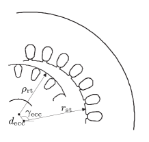
Figure 1: Eccentric geometry.

A magnetoquasistatic formulation based on the magnetic vector potential $\mathbf{A}$ is discretised at the 2D cross-sections $\Omega_{\text{st}}$ and $\Omega_{\text{rt}}$ by linear triangular finite elements (FEs) yielding a system of equations of the form

$$\mathbf{M}\frac{d}{dt}\mathbf{u}+\mathbf{K}\mathbf{u}+\mathbf{g}=\mathbf{f}$$ (2)

for each FE model part. In (2), $\mathbf{M}$ denotes the mass matrix related to the conductivity, $\mathbf{K}$ is the curl-curl stiffness matrix incorporating the reluctivity, $\mathbf{f}$ is the discretisation of the applied current density and $\mathbf{u}$ contains the degrees of freedom for the $z$-component of the magnetic vector potential. The contribution

$$\mathbf{g}_{i}=-\int_{\Gamma}H_{\theta}(\theta)N_{i}(\theta)\,\mbox{d}{\Gamma}$$ (3)

represent the magnetic field strength $H_{\theta}$ tangential to the interface $\Gamma$ weighted by the FE shape functions $N_{i}$. The two disconnected FE domains $\Omega_{\text{st}}$ and $\Omega_{\text{rt}}$ give raise to two decoupled FE systems of equations of the form (2) which are here distinguished by subscripts $\cdot_{\text{st}}$ and $\cdot_{\text{rt}}$. When $\Omega_{\text{ag}}=\emptyset$ and both FE model parts have a matching mesh at the common interface, the surface currents at the common boundary vanish, i.e., $\mathbf{g}_{\text{st}}+\mathbf{g}_{\text{rt}}=0$ and the standard FE system of equations can be obtained by combining both FE systems and eliminating the set of unknowns at one side of the interface. The time discretisation of (2) can be carried out by any time integration scheme.

The degrees of freedom for the $z$-component of the magnetic vector potential allocated at $\Gamma_{\text{st}}$ and $\Gamma_{\text{rt}}$ are collected in the vectors $\mathbf{\tilde{u}}_{\text{st}}$ and $\mathbf{\tilde{u}}_{\text{rt}}$ and are selected from the vectors $\mathbf{u}_{\text{st}}$ and $\mathbf{u}_{\text{rt}}$ by the rectangular selection matrices $\mathbf{Q}_{\text{st}}$ and $\mathbf{Q}_{\text{rt}}$, i.e., $\mathbf{\tilde{u}}_{\text{st}}=\mathbf{Q}_{\text{st}}\mathbf{u}_{\text{st}}$ and $\mathbf{\tilde{u}}_{\text{rt}}=\mathbf{Q}_{\text{rt}}\mathbf{u}_{\text{rt}}$.

3 Stator-Rotor Coupling

When classifying approaches for stator-rotor coupling according to the nature of the geometrical decomposition of the machine model, one can distinguish between sliding-surface and air-gap interface models.

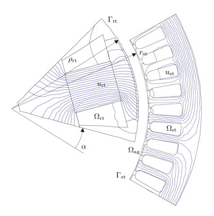
Figure 2: Computation domain $\Omega=\Omega_{\text{st}}\cup\Omega_{\text{ag}}\cup\Omega_{\text{rt}}$.

In sliding-surface techniques, the movement of the rotor is modelled at a common interface $\Gamma$ somewhere in the air gap. For the locked-step approach [21], an equidistant discretisation is applied at $\Gamma$ and the time step is chosen such that the rotor rotates with an integral number of mesh steps with respect to the stator. In general, the restriction to matching meshes is too severe for technical machine models. General sliding-surface techniques allow non-matching grids at $\Gamma$ and differ in the kind of interpolation which is applied at $\Gamma$, e.g. polynomial interpolation, mortar projection [23, 3] or trigonometric interpolation [9, 8].

In air-gap interface techniques, the air gap or a part of it is considered as a separate domain $\Omega_{\text{ag}}$ with an interface both to stator and rotor. The air-gap region is commonly discretised by a technique which allows a more convenient introduction of the relative motion than the standard FE method. Examples are the boundary integral method [24], the discontinuous Galerkin technique [2], the air-gap macro element [1] and a single-layer moving band [4, 10].

4 Air-Gap Element

The idea of the air-gap macro element is to model the air gap by a truncated series of sines and cosines which converges to the analytical solution if the number of FE vertices at $\Gamma_{\text{st}}$ and $\Gamma_{\text{rt}}$ tends to infinity [1, 17]. No additional degrees of freedom are introduced. The air-gap element is traditionally formulated as a particular transmission condition between the FE vertices at $\Gamma_{\text{st}}$ and $\Gamma_{\text{rt}}$. The air-gap element idea has been extended to higher-order elements [11] and anti-periodic boundary conditions [12]. Attempts to reduce the computational costs dedicated to the air-gap element are reported in [12].

This paper develops a general framework for the air-gap element wherein the formulations of [1], [17] and [12] are comprised. The paper frames the air-gap element within the more general theory of spectral-element methods and offers an at first sight more abstract but at the end more convenient notation. The more efficient implementation is different from the approaches in [1], [11] and [12] and involves a so-called variational crime, i.e., the weakening of the continuity conditions of the coupled discretisations. A major concern is to keep the computational cost of the air-gap macro element to a strict minimum.

The air-gap macro element is based on the analytical solution for the 2D magnetic vector potential $A_{z}$ in the air gap of the 2D cylindrical machine model

$$A_{{\rm ag},z}(r,\theta)=\mathbf{\underline{a}}_{0}+\mathbf{\underline{b}}_{0}\log\left(\frac{r}{\rho_{\text{rt}}}\right)$$ (4)

$$+\sum_{\lambda\in\Lambda}\left(\mathbf{\underline{a}}_{\lambda}\left(\frac{r}{\rho_{\text{rt}}}\right)^{\lambda}+\mathbf{\underline{b}}_{\lambda}\left(\frac{r}{\rho_{\text{rt}}}\right)^{-\lambda}\right)e^{-\jmath\lambda\theta}$$

where $\mathbf{\underline{a}}_{\lambda}$ and $\mathbf{\underline{b}}_{\lambda}$ are complex-valued coefficients and $\lambda\in\Lambda$ is the harmonic order. The air-gap element considers a finite set $\Lambda$ of harmonic orders. In the formulation developed here, the component with $\lambda=0$ is not considered. Instead, it is assumed that a Dirichlet boundary condition is applied at both the stator and rotor sides such that the arbitrary constant of $A_{z}$ is defined. In the case of a real-valued formulation, $u(r,\theta)$ is real and hence $a_{-\lambda}=a_{\lambda}^{*}$ and $b_{-\lambda}=b_{\lambda}^{*}$ where ^∗ stands for conjugate or conjugate transpose for variables and matrices respectively. Notice that by inserting Le Moivre’s formula, i.e., $e^{-\lambda p\lambda\theta}=\cos{p\lambda\theta}-\jmath\sin{p\lambda\theta}$, the notation of [1], [11] and [12] is regained. The magnetic field strength in the $\theta$-direction is computed from (4):

$$H_{{\rm ag},\theta}(r,\theta)=\mathbf{\underline{b}}_{0}\frac{\nu_{0}}{r}$$ (5)

$$+\sum_{\lambda\in\Lambda}\frac{\nu_{0}\lambda}{r}\left(\mathbf{\underline{a}}_{\lambda}\left(\frac{r}{\rho_{\text{rt}}}\right)^{\lambda}-\mathbf{\underline{b}}_{\lambda}\left(\frac{r}{\rho_{\text{rt}}}\right)^{-\lambda}:\right)e^{-\jmath\lambda\theta}\;.$$

The air-gap fields (4) and (5), evaluated at $\Gamma_{\text{st}}$ and $\Gamma_{\text{rt}}$, are matched to harmonic decomposition at the interfaces, e.g.

$$A_{{\rm st},z} = \sum_{\lambda\in\Lambda}\mathbf{\underline{c}}_{{\rm st},\lambda}e^{-\jmath\lambda\theta}\;;$$ (6)

$$H_{{\rm st},\theta} = \sum_{\lambda\in\Lambda}\mathbf{\underline{d}}_{{\rm st},\lambda}e^{-\jmath\lambda\theta}\;.$$ (7)

The coefficients $\mathbf{\underline{c}}_{\text{st}}$ and $\mathbf{\underline{c}}_{\text{rt}}$ are related to $\mathbf{\underline{a}}$ and $\mathbf{\underline{b}}$ by

$$\left[\begin{array}[]{c}\mathbf{\underline{c}}_{\text{st}}\\ \mathbf{\underline{c}}_{\text{rt}}\end{array}\right]=\mathbf{T}\left[\begin{array}[]{c}\mathbf{\underline{a}}\\ \mathbf{\underline{b}}\end{array}\right]$$ (8)

where $\mathbf{T}$ is a block-diagonal matrix of which the blocks $\mathbf{T}_{\lambda}$ and $\mathbf{T}_{0}$ are defined by

$$\mathbf{T}_{\lambda} = \left[\begin{array}[]{cc}\xi^{\lambda}&\xi^{-\lambda}\\ 1&1\end{array}\right]\;;$$ (11)

$$\mathbf{T}_{0} = \left[\begin{array}[]{cc}1&\ln{\xi}\\ 1&0\end{array}\right]$$ (14)

and $\xi=r_{\text{st}}/\rho_{\text{rt}}$ denotes the air-gap radius ratio. The coefficients $\mathbf{\underline{d}}_{\text{st}}$ and $\mathbf{\underline{d}}_{\text{rt}}$ are related to $\mathbf{\underline{a}}$ and $\mathbf{\underline{b}}$ by

$$\left[\begin{array}[]{c}\mathbf{\underline{d}}_{\text{st}}\\ \mathbf{\underline{d}}_{\text{rt}}\end{array}\right]=\mathbf{G}\left[\begin{array}[]{c}\mathbf{\underline{a}}\\ \mathbf{\underline{b}}\end{array}\right]$$ (15)

where $\mathbf{G}$ is a block-diagonal matrix of which the blocks $\mathbf{G}_{\lambda}$ are defined by

$$\mathbf{G}_{\lambda}=\nu_{0}\lambda\left[\begin{array}[]{cc}-\xi^{\lambda}/r_{\text{st}}&\xi^{-\lambda}/r_{\text{st}}\\ -1/\rho_{\text{rt}}&1/\rho_{\text{rt}}\end{array}\right]$$ (16)

where $\nu_{0}$ denotes the reluctivity of air. The air-gap element provides a so-called spectral Dirichlet-to-Neumann operator $\mathbf{G}\mathbf{T}^{-1}$

$$\left[\begin{array}[]{c}\mathbf{\underline{d}}_{\text{st}}\\ \mathbf{\underline{d}}_{\text{rt}}\end{array}\right]=\mathbf{G}\mathbf{T}^{-1}\left[\begin{array}[]{c}\mathbf{\underline{c}}_{\text{st}}\\ \mathbf{\underline{c}}_{\text{rt}}\end{array}\right]$$ (17)

mapping the harmonic coefficients for the magnetic vector potential upon the corresponding harmonic coefficients for the magnetic field strengths at $\Gamma_{\text{st}}$ and $\Gamma_{\text{rt}}$.

5 Coupling with FE Model Parts

The air-gap element is matched to the FE solutions at the interfaces $\Gamma_{\text{st}}$ and $\Gamma_{\text{rt}}$. The necessary interface conditions for $A_{z}$ and $H_{\theta}$ are applied in a weak way, i.e., by multiplying with test functions $w_{p}(\theta)$ and $v_{\zeta}(\theta)$, e.g. at $\Gamma_{\text{st}}$

$$\int_{\Gamma_{\text{st}}}\left(A_{{\rm st},z}(r_{\text{st}},\theta)-A_{{\rm ag},z}(r_{\text{st}},\theta)\right)w_{p}(\theta)\,\mbox{d}{\Gamma} = 0\;;$$ (18)

$$\int_{\Gamma_{\text{rt}}}\left(H_{{\rm st},\theta}(r_{\text{st}},\theta)-H_{{\rm ag},\theta}(r_{\text{st}},\theta)\right)v_{\zeta}(\theta)\,\mbox{d}{\Gamma} = 0\;.$$ (19)

In combination with appropriate test functions, (18) and (19) correspond to the mortar element approach [3]. The particular choice for test and trial functions made here, however, corresponds to pointwise matching at the vertices of the FE meshes:

$$w_{p}(\theta) = \delta_{p}(\theta)\;;$$ (20)

$$v_{\zeta}(\theta) = e^{\jmath\zeta\theta}\;;$$ (21)

$$h_{q}(\theta) = \delta_{q}(\theta)\;,$$ (22)

where the delta function $\delta_{p}(\theta)$ is defined such that $\delta_{p}(\theta)$ is only non-zero at $\theta=\theta_{p}$ and its integral over $\Gamma_{\text{st}}$ or $\Gamma_{\text{rt}}$ equals $2\pi r_{\text{st}}$ or $2\pi\rho_{\text{rt}}$ respectively. The choices for $w_{p}(\theta)$ and $h_{q}(\theta)$ in (18) and (19) are such that the Fast Fourier Transform (FFT) algorithm can be used for turning the FE degrees of freedom into the harmonic coefficients and otherwise:

$$\left[\begin{array}[]{cc}\mathbf{\underline{c}}_{\text{st}}\\ \mathbf{\underline{c}}_{\text{rt}}\end{array}\right] = \left[\begin{array}[]{cc}\mathbf{F}&0\\ 0&\mathbf{F}\end{array}\right]\left[\begin{array}[]{cc}\mathbf{\tilde{u}}_{\text{st}}\\ \mathbf{\tilde{u}}_{\text{rt}}\end{array}\right]\;;$$ (29)

$$\left[\begin{array}[]{cc}\mathbf{\tilde{g}}_{\text{st}}\\ \mathbf{\tilde{g}}_{\text{rt}}\end{array}\right] = \left[\begin{array}[]{cc}\mathbf{F}^{-1}&0\\ 0&\mathbf{F}^{-1}\end{array}\right]\left[\begin{array}[]{cc}\mathbf{\underline{d}}_{\text{st}}\\ \mathbf{\underline{d}}_{\text{rt}}\end{array}\right]$$ (36)

where $\mathbf{F}$ denotes the FFT. Pointwise matching is a collocation approach for which it is known that the discretisation error convergence less favourably as for the FE method. In the following, matrices for the stator and rotor part combined into block-diagonal matrices are denoted similarly, but without subscript, i.e.,

$$\mathbf{K}=\left[\begin{array}[]{cc}\mathbf{K}_{\text{st}}&0\\ 0&\mathbf{K}_{\text{rt}}\end{array}\right]\;.$$ (37)

The combination of (2), (17), (29) and (36) results in the coupled FE-SE system of equations

$$\mathbf{M}\frac{d}{dt}\mathbf{u}+\mathbf{K}\mathbf{u}+\mathbf{Q}^{T}\mathbf{F}^{-1}\mathbf{G}\mathbf{T}^{-1}\mathbf{F}\mathbf{Q}\mathbf{u}=\mathbf{f}\;.$$ (38)

Despite of the asymmetrical notation in (38), it is easy to prove that the air-gap stiffness matrix part

$$\mathbf{K}_{\text{ag}}=\mathbf{Q}^{T}\mathbf{F}^{-1}\mathbf{G}\mathbf{T}^{-1}\mathbf{F}\mathbf{Q}$$ (39)

is a symmetric and real-valued operator. The symmetry follows from the symmetry of the 2-by-2 diagonal blocks of $\mathbf{G}\mathbf{T}^{-1}$ and the fact that $\mathbf{F}^{H}=n\mathbf{F}^{-1}$ with $n$ the number of vertices at the interfaces. Moreover, real-valued field distributions $\mathbf{\tilde{u}}_{\text{st}}$ and $\mathbf{\tilde{u}}_{\text{rt}}$ are transformed into harmonic components which satisfy $\mathbf{\underline{c}}_{{\rm st},-\lambda}=\overline{\mathbf{\underline{c}}_{{\rm st},\lambda}}$. This property is maintained by the spectral Dirichlet-to-Neumann operator $\mathbf{G}\mathbf{T}^{-1}$ from which can be concluded that $\mathbf{K}_{\text{ag}}$ will return a real-valued vector.

The air-gap stiffness matrix $\mathbf{K}_{\text{ag}}$ contains a dense block of dimension $2n\times 2n$. Hence, the insertion of $\mathbf{K}_{\text{ag}}$ as an algebraic matrix into the FE system matrix would cause a significant fill-in (Fig. 3).

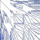
(a)       (b)

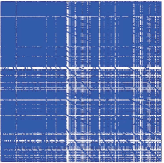
Figure 3: Sparsity patterns of (a) $\beta\mathbf{M}+\mathbf{K}$ (224172 nonzeros) and (b) $\mathbf{A}=\beta\mathbf{M}+\mathbf{K}+\mathbf{K}_{\text{ag}}$ (809040 nonzeros) where $\beta$ is a factor determined by the time integration method.

This is not a problem for a relatively small machine model, when sufficient memory is available and direct system solution techniques can be applied. For larger machine model, however, the more expensive matrix-vector product leads to huge computation times if standard iterative solution techniques are used. Therefore, the explicit construction of $\mathbf{K}_{\text{ag}}$ as an algebraic matrix should be avoided by all means.

6 Rotation

When the rotor is rotated around its axis by an angle $\alpha$, the new local coordinate system reads $(\rho,\varphi^{\prime})$ where $\varphi^{\prime}=\varphi-\alpha$. The harmonic coefficients $\mathbf{\underline{c}}^{\prime}_{\text{rt}}$ with respect to $(\rho,\varphi^{\prime})$ are related to $\mathbf{\underline{c}}_{\text{rt}}$ by $\mathbf{\underline{c}}_{\text{rt}}=\mathbf{R}_{-\alpha}\mathbf{\underline{c}}^{\prime}_{\text{rt}}$ where $\mathbf{R}_{-\alpha}$ is a diagonal matrix containing the phasors

$$\mathbf{R}_{-\alpha,\lambda,\lambda}=e^{\jmath\lambda\alpha}\;.$$ (40)

This remarkably simple way to account for rotor displacement is particularly advantageous in case of transient simulation. Using this extended air-gap model, there is no longer need to rotate the rotor mesh while time-stepping. It is sufficient to adapt the rotation matrix $\mathbf{R}_{-\alpha}$ in the formulation to the actual angular rotor position. The astonishing simplicity of considering rotor motion is one of the major advantages of the air-gap element [8, 7].

7 Rotor or Stator Skewing

Rotor or stator skewing is commonly introduced in 2D machine models by considering multiple slices at different axial positions of the machine. The different slices are connected by the external electric circuit [19, 16]. It is possible to account for the skewing even if only 1 slice is modelled when the spatial harmonic decomposition of the air-gap field is available [6]. The harmonic coefficients at one of the interfaces, e.g. at $\Gamma_{\text{st}}$, are multiplied by analytical skew factors depending on the skew angle $\gamma_{\text{skew}}$: $\mathbf{\underline{c}}^{\prime}_{\text{st}}=\mathbf{S}_{\text{skew}}\mathbf{\underline{c}}_{\text{st}}$ where

$$\mathbf{S}_{{\rm skew},\lambda,\lambda}=\frac{2}{\lambda\gamma_{\text{skew}}}\sin\left(\frac{\lambda\gamma_{\text{skew}}}{2}\right)\;.$$ (41)

Nevertheless, multiple slices have to be considered in order to deal with the axial variation of the ferromagnetic saturation. In that case, the skew angle of each slice is $\gamma_{\text{skew}}\ell_{z,q}/\ell_{z}$ where $\ell_{z,q}$ and $\ell_{z}$ are the axial length of slice $q$ and of the entire machine respectively.

8 Static and Dynamic Eccentricity

In case of an eccentric rotor, the coordinate transformation (1) is introduced in the air-gap element formula (4). The nested loop is rearranged into increasing powers of $\rho$. It may be assumed that the magnitude of the eccentricity is small compared to the radius of the rotor, i.e., $\varepsilon=d_{\text{ecc}}/\rho_{\text{rt}}\ll 1$. Then, all higher-order contributions $\varepsilon^{k}$ starting from $k=2$ can be neglected in the series expansion:

$$A_{z}(\rho,\varphi)$$ (42)

$$=\sum_{\lambda\in\Lambda}\Big{[}\left(\frac{\rho}{\rho_{\text{rt}}}\right)^{\lambda}\left(\mathbf{\underline{a}}_{\lambda}+(\lambda+1)\varepsilon_{\text{ecc}}e^{-\jmath\gamma_{\text{ecc}}}\mathbf{\underline{a}}_{\lambda+1}\right)$$

$$+\left(\frac{\rho}{\rho_{\text{rt}}}\right)^{-\lambda}\left(\mathbf{\underline{b}}_{\lambda}-(\lambda-1)\varepsilon_{\text{ecc}}e^{\jmath\gamma_{\text{ecc}}}\mathbf{\underline{b}}_{\lambda-1}\right)\Big{]}e^{-\jmath\lambda\varphi}$$

$$+\mathcal{O}\left(\varepsilon_{\text{ecc}}^{2}\right)\;.$$

The relative eccentricity and the eccentricity angle are combined in a single complex number $\underline{\varepsilon}_{\text{ecc}}=\varepsilon_{\text{ecc}}e^{\jmath\gamma_{\text{ecc}}}$. The azimuthal magnetic field strength with respect to the rotor coordinate system $(\rho,\varphi)$ reads

$$H_{\varphi}(\rho,\varphi)$$ (43)

$$=\sum_{\lambda\in\Lambda}\frac{\nu_{0}\lambda}{\rho}\Big{[}\left(\frac{\rho}{\rho_{\text{rt}}}\right)^{\lambda}\left(\mathbf{\underline{a}}_{\lambda}+(\lambda+1)\overline{\underline{\varepsilon}_{\text{ecc}}}\;\mathbf{\underline{a}}_{\lambda+1}\right)$$

$$-\left(\frac{\rho}{\rho_{\text{rt}}}\right)^{-\lambda}\left(\mathbf{\underline{b}}_{\lambda}-(\lambda-1)\underline{\varepsilon}_{\text{ecc}}\;\mathbf{\underline{b}}_{\lambda-1}\right)\Big{]}e^{-\jmath\lambda\varphi}$$

$$+\mathcal{O}\left(\varepsilon_{\text{ecc}}^{2}\right)\;.$$

The eccentricity is modelled as a perturbation of the classical air-gap macro element [15]. The matrices $\mathbf{T}_{\underline{\varepsilon}}$ and $\mathbf{G}_{\underline{\varepsilon}}$ are tri-diagonal block matrices where the diagonal blocks are the same as in $\mathbf{T}$ and $\mathbf{G}$ and the off-diagonal blocks are obtained by writing (42) and (43) for $\rho=\rho_{\text{rt}}$ and collecting the appropriate coefficients. An eccentric air-gap element is obtained by replacing $\mathbf{T}$ and $\mathbf{G}$ in (8) and (15) by $\mathbf{T}_{\underline{\varepsilon}}$ and $\mathbf{G}_{\underline{\varepsilon}}$.

9 Arbitrary FE Meshes at $\Gamma_{\text{st}}$ and $\Gamma_{\text{rt}}$

The assumption that the FE meshes at $\Gamma_{\text{st}}$ and $\Gamma_{\text{rt}}$ should be equidistant and should have the same number of nodes, is too restrictive for technically relevant models. The classical FFT algorithm, however, dictates the uniform distribution of FE vertices at $\Gamma_{\text{st}}$ and $\Gamma_{\text{rt}}$. Recently, FFT algorithms for non-equispaced data are developed [20]. Their application is slightly more expensive compared to the classical FFT algorithm. The computational complexity, however, remains $\mathcal{O}(n\log n)$ such that the overall computation time of the FE simulation is barely influenced by the application of the air-gap element. When different numbers of FE vertices are applied at $\Gamma_{\text{st}}$ and $\Gamma_{\text{rt}}$, the sets of harmonic orders present in $\mathbf{\underline{c}}_{\text{st}}=\mathbf{F}_{\text{st}}\tilde{\mathbf{u}}_{\text{st}}$ and $\mathbf{\underline{c}}_{\text{rt}}=\mathbf{F}_{\text{rt}}\tilde{\mathbf{u}}_{\text{rt}}$, denoted by $\Lambda_{\text{st}}$ and $\Lambda_{\text{rt}}$ respectively, are different. The coupling through the eccentric air-gap element is only applied for a user-defined subset of the available components: $\Lambda\subset\Lambda_{\text{st}}\cup\Lambda_{\text{rt}}$. The selectors $\mathbf{X}_{\text{st}}$ and $\mathbf{X}_{\text{rt}}$ select the harmonic coefficients with orders $\lambda\in\Lambda$ from $\mathbf{\underline{c}}_{\text{st}}$ and $\mathbf{\underline{c}}_{\text{rt}}$ respectively. Only these components are treated by the modified air-gap reluctance matrix:

$$\mathbf{K}_{\text{ag}}=\mathbf{Q}^{T}\mathbf{F}^{-1}\mathbf{X}^{T}\mathbf{G}\mathbf{T}^{-1}\mathbf{X}\mathbf{F}\mathbf{Q}\;.$$ (44)

The harmonic coefficients which are not considered by the air-gap element are not influenced by the air-gap and experience homogeneous Neumann boundary conditions at $\Gamma_{\text{st}}$ and $\Gamma_{\text{rt}}$.

10 Procedure

After introduction of rotation, skewing and eccentricity, the air-gap stiffness matrix reads

$$\mathbf{K}_{\text{ag}}=\mathbf{Q}^{T}\mathbf{F}^{-1}\mathbf{X}^{T}\mathbf{R}_{\alpha}\mathbf{S}_{\text{skew}}\mathbf{G}_{\underline{\varepsilon}}\mathbf{T}_{\underline{\varepsilon}}^{-1}\mathbf{S}_{\text{skew}}\mathbf{R}_{-\alpha}\mathbf{X}\mathbf{F}\mathbf{Q}\;.$$ (45)

The heavy matrix notation used for developing the air-gap element in the previous sections is misleading. The application of the air-gap element as a procedure acting upon the distributions of the magnetic vector potential at $\Gamma_{\text{st}}$ and $\Gamma_{\text{rt}}$ provides both a better understanding and a more efficient algorithm. The air-gap element computes the surface currents $\mathbf{\tilde{g}}_{\text{st}}$ and $\mathbf{\tilde{g}}_{\text{rt}}$ occurring at $\Gamma_{\text{st}}$ and $\Gamma_{\text{rt}}$ for particular field distributions $\mathbf{\tilde{u}}_{\text{st}}$ and $\mathbf{\tilde{u}}_{\text{rt}}$ applied at the same boundaries. The procedure for explicitly carrying out this computation is depicted in Fig. 4.

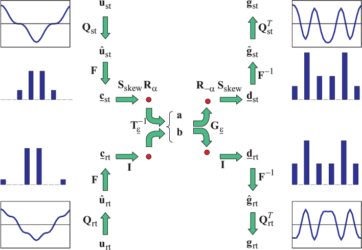
Figure 4: Procedure to apply the eccentric air-gap element coupling the FE model parts of stator and rotor.

• Given a temporary FE solution vector $[\mathbf{u}_{\text{st}}\;\mathbf{u}_{\text{rt}}]^{T}$ for the magnetic vector potentials in $\Omega_{\text{st}}$ and $\Omega_{\text{rt}}$, the values at the air-gap interfaces $\Gamma_{\text{st}}$ and $\Gamma_{\text{rt}}$ are selected by the selection matrices $\mathbf{Q}_{\text{st}}$ and $\mathbf{Q}_{\text{rt}}$, yielding $\mathbf{\tilde{u}}_{\text{st}}$ and $\mathbf{\tilde{u}}_{\text{rt}}$. This operations are implemented on a computer by subscripting the FE solution vectors by predefined index sets.

• The vectors of harmonics $\mathbf{\underline{c}}_{\text{st}}$ and $\mathbf{\underline{c}}_{\text{rt}}$ are obtained by applying Fast Fourier Transforms to $\mathbf{\tilde{u}}_{\text{st}}$ and $\mathbf{\tilde{u}}_{\text{rt}}$. The FFTW algorithm which is used for that purpose, consists of a setup step, which is only carried out once, and a computation step which has to be invoked 4 times per application of $\mathbf{K}_{\text{ag}}$ [14].

• At one of both sides, the rotation operator $\mathbf{R}_{-\alpha}$ and the skewing operator $\mathbf{S}_{\text{skew}}$ are applied. This corresponds to a vector-vector multiplication by phasors and scaling factors respectively.

• From the (modified) harmonic coefficients $\mathbf{\underline{c}}_{\text{st}}$ and $\mathbf{\underline{c}}_{\text{rt}}$ related to the magnetic vector potential distribution at $\Gamma_{\text{st}}$ and $\Gamma_{\text{rt}}$, the harmonic coefficients $\mathbf{\underline{d}}_{\text{st}}$ and $\mathbf{\underline{d}}_{\text{rt}}$ related to the fictitious surface currents at $\Gamma_{\text{st}}$ and $\Gamma_{\text{rt}}$ are computed by applying the precomputed 2-by-2 blocks $\mathbf{G}_{\lambda}\mathbf{T}_{\lambda}^{-1}$ or in the eccentric case by applying $\mathbf{G}_{\underline{\varepsilon}}\mathbf{T}_{\underline{\varepsilon}}^{-1}$.

• The discretized surface currents $\mathbf{\tilde{g}}_{\text{st}}$ and $\mathbf{\tilde{g}}_{\text{rt}}$ at $\Gamma_{\text{st}}$ and $\Gamma_{\text{rt}}$ follow by an inverse Fourier transformation applied to $\mathbf{\underline{d}}_{\text{st}}$ and $\mathbf{\underline{d}}_{\text{rt}}$.

• Finally, $\mathbf{\tilde{u}}_{\text{st}}$ and $\mathbf{\tilde{u}}_{\text{rt}}$ are prolongated to vectors according to the FE problems by computing $\mathbf{g}_{\text{st}}=\mathbf{Q}_{\text{st}}^{T}\mathbf{\tilde{g}}_{\text{st}}$ and $\mathbf{g}_{\text{rt}}=\mathbf{Q}_{\text{rt}}^{T}\mathbf{\tilde{g}}_{\text{rt}}$ again by invoking subscripting using appropriate index sets on the computer.

This procedure is made available as a separate software routine

$$\mathtt{g=airgapelement(u,alpha,gammaskew,decc,gecc)}$$ (46)

taking the vectors $\mathbf{u}_{\text{st}}$ and $\mathbf{u}_{\text{rt}}$, the rotation angle $\alpha(t)$, the skew angle $\gamma_{\text{skew}}$ and the magnitude $d_{\text{ecc}}(t)$ and angle $\gamma_{\text{ecc}}(t)$ of the eccentricity as parameters and returning the vectors $\mathbf{g}_{\text{st}}$ and $\mathbf{g}_{\text{rt}}$.

11 Discretisation and Consistency Errors

11.1 Discretisation error of the air-gap element

When the range of the harmonic orders $\lambda$ is limited to $\Lambda$ instead of $\lambda\in\{,-\infty,\ldots,+\infty\}$ as for the analytical model, a truncation error is introduced. The analytical air-gap solution is equivalent to a spectral element (SE) discretization using an orthogonal set of harmonic functions as test and trial functions [13]. The SE approach is known to achieve an exponential convergence rate of the discretization error as long as no sharp corners and no jumps of the material coefficients are present in the SE model part, which is the case for the air gap of an electrical machine. Hence, the overall discretization error of the coupled FE-SE formulation will be dominated by the discretization error of the FE model parts and the consistency error introduced by the non-matching discretizations at $\Gamma_{\text{st}}$ and $\Gamma_{\text{rt}}$.

11.2 Consistency error at the interfaces

A consistency error is introduced by the choice of non-matching shape functions for $A_{z}$ and $H_{\theta}$ at the interfaces. It is shown in literature dealing with the mortar-element method (see e.g. [22]) that the consistency error at $\Gamma_{\text{st}}$ and $\Gamma_{\text{rt}}$ may have a lower convergence rate than the one for the FE and SE discretizations at $\Omega_{\text{st}}$, $\Omega_{\text{rt}}$ and $\Omega_{\text{ag}}$, which leads to a degenerated convergence of the overall discretization error for the hybrid model. Moreover, for triangulations of cylindrical machines, $\Gamma_{\text{st}}$ and $\Gamma_{\text{rt}}$ are polygons instead of circles such that the hybrid integrals in (18) and (19) connect the SE degrees of freedom not only to the FE degrees of freedom at the nodes of the interfaces but also to the FE degrees of freedom associated with the first layer of nodes inside $\Omega_{\text{st}}$ and $\Omega_{\text{rt}}$ [22]. The approach in [22] offers a better convergence of the consistency error but causes a substantial increase of the computational work, especially because FFT is not longer applicable. An acceptable trade-off consists of integrating the interface conditions at the circles $r=r_{\text{st}}$ and $\rho=\rho_{\text{rt}}$ and assuming a linear variation of the FE shape functions at the circle segments. This improvement is introduced in the formulation described above by replacing $\mathbf{F}$ by $\mathbf{S}_{\rm int}\mathbf{F}$ where

$$\mathbf{S}_{{\rm int},\lambda,\lambda}=\frac{2n}{\lambda}\sin(\frac{\lambda}{2n})\;.$$ (47)

This approach exactly corresponds to the original macro element [1]. By substituting $\cos{\lambda\theta}-\jmath\sin{\lambda\theta}$ for $e^{-\jmath\lambda\theta}$, the notation used in [1] and [12] is achieved.

11.3 Stability

For a stable numerical approach, arbitrarily small differences in the results can be uniformly bounded by arbitrarily small differences in the input data. When simulating solid-body motion, the modelling of the geometrical changes is an important part of the simulation scheme. When using a moving-band technique, the moving band is remeshed between two successive simulation steps. An arbitrary small displacement of the rotor (either rotation or eccentricity) can result in a topological change of the FE mesh, e.g. a different number of FE vertices or an edge that is oriented otherwise (Fig. 5).

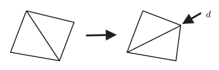
Figure 5: Topological change of the FE mesh due to a small displacement of a part of the model. The displacement $d$ of one node belonging to the rotor causes a small distortion of a quadrilateral consisting of two triangles in the moving band. The diagonal edge of the original mesh is now shorter than the edge between the two other opposite nodes. In that case, the Delaunay mesh procedure selects the other diagonal as a division of the quadrangle into two triangles and thereby changes the topology of the mesh.

Hence, the remeshing of the moving band is not stable with respect to the solid-body displacement of the rotor, i.e., there does not exist a constant $C<\infty$ such that

$$\left\|\mathbf{u}(d)-\mathbf{u}(0)\right\|<C\|d\|,\quad\forall\|d\|>0$$ (48)

where $\mathbf{u}(d)$ represent the FE solution for a solid-body displacement $d$. Such changes have a significant influence upon the computed FE solutions. As a consequence, it is not always possible to obtain an arbitrary small difference between two successive FE solutions even if a very small displacement $d$ is applied. A similar phenomenon is reported as torque ripple when simulating rotating machines using the moving-band approach [27]. The moving-band technique has been generalized for FE machine models with static and dynamic eccentricity [5, 26]. Although a moving-band approach which is stable with respect to eccentricity has been developed [25], the stability with respect to rotation is still not given. This phenomenon is particularly annoying when the displacements are smaller than the FE mesh size, as is commonly the case when accounting for eccentricity in FE machine models. One of the major benefits of the eccentric air-gap element, is the guaranteed stability of the air-gap discretization with respect to small displacements of the rotor. This property is indispensable to ensure a reliable torque and force computation.

12 Iterative Solution

The assembly of $\mathbf{K}_{\text{ag}}$ into $\beta\mathbf{M}+\mathbf{K}$ drastically increases the density of the matrix and, as a consequence, will decrease the numerical efficiency of the air-gap element approach. To our opinion, this is the major reason why the air-gap element approach is not so widespread as the moving-band technique. Here, an iterative approach is proposed which alleviates this problem. The key point is that the air-gap stiffness matrix is not assembled into the FE system matrix. Instead, the air-gap stiffness matrix $\mathbf{K}_{\text{ag}}$ is provided as a routine (46) turning an arbitrary vector $\mathbf{u}$ of FE degrees of freedom into the corresponding surface currents $\mathbf{g}$ reflecting the reluctance of the air gap as illustrated by Fig. 4. At the $k$-th CG step, the matrix-vector product $\mathbf{f}_{k}=\mathbf{A}\mathbf{u}_{k}$ is carried out by adding the contribution of the conventional matrix-vector product of $\mathbf{u}_{k}$ by $\beta\mathbf{M}+\mathbf{K}$ and the vector $\mathbf{g}_{k}$ obtained by applying the routine (46) to $\mathbf{u}_{k}$. The operations in (39) needed to compute $\mathbf{g}_{k}$ from $\mathbf{u}_{k}$ are applied successively as depicted in Fig. 4. By applying the Fast Fourier Transform (FFT) algorithm for $\mathbf{F}$ and $\mathbf{F}^{-1}$, the computational cost of the discrete Fourier transforms, and thus of the eccentric air-gap element, can be kept as low as $\mathcal{O}(n\log{n})$. The application of FFT is absolutely necessary to ensure that the eccentric air-gap element is competitive to moving-band and sliding-surface approaches [7]. Inserting the operator (39) and combining real-valued and complex-valued arithmetic is not possible in many black-box CG solvers. Hence, a specialized CG algorithm has to be developed, which is the major disadvantage of the improved air-gap element approach described here.

The convergence of CG can be improved considerably by applying preconditioning. Since no algebraic matrix representing $\mathbf{A}$ is available, pure algebraic preconditioning techniques such as e.g. Successive Overrelaxation, Incomplete Cholesky and Algebraic Multigrid (AMG) are not applicable [7]. A straightforward preconditioner is e.g. an additive Schwarz approach

$$(\mathbf{I}-\mathbf{Q})^{T}\tilde{\mathbf{A}}^{-1}(\mathbf{I}-\mathbf{Q})+\mathbf{Q}^{T}\mathbf{F}^{-1}\mathbf{T}_{\underline{\varepsilon}}\mathbf{G}_{\underline{\varepsilon}}^{-1}\mathbf{F}\mathbf{Q}$$ (49)

where $\tilde{\mathbf{A}}^{-1}$ denotes the application of 1 V-cycle of AMG. Also the preconditioning step involves operations defined by a routine similar to (46).

Special care has to be taken if the constant components $\mathbf{\underline{a}}_{0}+\mathbf{\underline{b}}_{0}\log(r/\rho_{\text{rt}})$ are considered in the air-gap element. The solution for $A_{z}$ is known up to a constant field. When e.g. only Dirichlet constraints are applied to the stator model part, $\mathbf{K}_{\text{rt}}$ is singular and the constant at the rotor side should be fixed by the air-gap element formulation. Then, a problem rises for the magnetic field strength because $\mathbf{G}_{0}$ is a singular matrix. $\mathbf{K}_{\text{ag}}^{-1}$ is not defined for the constant components such that the analytical formulae (4) and (5) fail to compute $\mathbf{\underline{d}}_{{\rm st},0}$ and $\mathbf{\underline{d}}_{{\rm rt},0}$ from $\mathbf{\underline{c}}_{{\rm st},0}$ and $\mathbf{\underline{c}}_{{\rm rt},0}$. The constant component of the magnetic field strength is determined by the total current $i_{\text{rt}}$ through the rotor:

$$H_{{\rm st},\theta} = \frac{i_{\text{rt}}}{2\pi r_{\text{st}}}$$ (50)

$$H_{{\rm rt},\theta} = \frac{i_{\text{rt}}}{2\pi\rho_{\text{rt}}}$$ (51)

which necessitates the coupling of the air-gap element to the degrees of freedom of the external circuit model. An easier procedure consists of applying at least one Dirichlet boundary condition at the rotor side and replacing the 2-by-2 block matrices $\mathbf{G}_{0}\mathbf{T}_{0}^{-1}$ and $\mathbf{T}_{0}\mathbf{G}_{0}^{-1}$ by zero matrices such that no constant components have to be propagated through the air-gap model. This approach is, however, not applicable for machine models where the total current through the rotor does not vanish.

13 Torque and Unbalanced Magnetic Pull

When the air-gap harmonics are available, a highly accurate value for the torque can be computed using the formula [18]

$$T=\sum_{\lambda\in\Lambda}8\pi\nu_{0}\ell_{z}{\rm Im}\left\{\mathbf{\underline{a}}^{H}\mathbf{\underline{b}}\right\}\;.$$ (52)

Thanks to the stability of the air-gap element approach, torque ripple is avoided [9].

The availability of the harmonic coefficients of the air-gap field also allows to compute the unbalanced magnetic pull up to the highest possible accuracy achieved by the FE model. The magnetic flux density $(B_{r},B_{\theta})$ with respect to the standstill polar coordinate system can be gathered into a complex-valued field:

$$\underline{B}=B_{r}+\jmath B_{\theta}=\sum_{\lambda\in\Lambda}\frac{-\jmath\lambda}{r}2\mathbf{\underline{a}}_{\lambda}\left(\frac{r}{\rho_{\text{rt}}}\right)^{\lambda}e^{-\jmath\lambda\theta}\;.$$ (53)

Similarly, the force components $F_{x}$ and $F_{y}$, expressed by the Maxwell stress tensor, can be brought together:

$$\underline{F}=F_{x}+\jmath F_{y}=\ell_{z}\int_{0}^{2\pi}\frac{\nu_{0}}{2}\underline{B}^{2}e^{\jmath\theta}r\,\mbox{d}{\theta}\;.$$ (54)

Introducing (53) into (54) and working out the integral leads to

$$\underline{F}=-\frac{4\pi\ell_{z}\nu_{0}}{\rho_{\text{rt}}}\sum_{\lambda\in\Lambda}\lambda(1-\lambda)\mathbf{\underline{a}}_{\lambda}\mathbf{\underline{a}}_{1-\lambda}\;.$$ (55)

14 Example

The 2D FE model of a magnetic bearing (Fig. 6a) is equipped with the eccentric air-gap element.

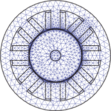
(a)            (b)            (c)

Figure 6: Magnetic-bearing model: (a) FE mesh; (b) magnetic flux lines (unbiased excitation) and (c) magnetic flux lines (biased excitation).

Transient simulations are carried out to test the numerical behaviour of the eccentric air-gap element and the embedded force computation. The rotor is submitted to a prescribed movement which is a combination of a translation from the position $(0.5\;\mathrm{mm},9\pi/8)$ to the position $(0.5\;\mathrm{mm},\pi/8)$ and a rotation around its axis. The stator coils are excited such that a force under an angle of $22.5$ degrees is generated. Both unbiased and biased current excitations are considered. The magnetic fluxes when the rotor is at the center position are shown for both unbiased and biased excitation in Fig. 6.

During the transient simulation, the stator and rotor FE meshes do not have to be reconstructed. The movement of the rotor between two successive time steps only affect the operators $\mathbf{T}_{\underline{\varepsilon}}$, $\mathbf{G}_{\underline{\varepsilon}}$ and $\mathbf{R}_{\alpha}$ which are embedded in the eccentric air-gap stiffness operator $\mathbf{K}_{\text{ag}}$. In practice, only the parameters specified in the routine (46) have to be adapted. The FE systems $\beta\mathbf{M}_{\text{st}}+\mathbf{K}_{\text{st}}$ and $\beta\mathbf{M}_{\text{rt}}+\mathbf{K}_{\text{rt}}$ are only reassembled as to account for the saturation of the ferromagnetic parts. The AMG preconditioner is only constructed once before starting the time-stepping procedure. The formulation based on the eccentric air-gap element substantially diminishes the time for system set-up during the transient simulation. No ripple on the results for the force is encountered, indicating the stability of the discretization scheme with respect to small displacements.

15 Conclusions

The reformulation of the air-gap element and its interpretation as a spectral-element discretisation in the air gap leads to a formulation for which the major part of the work can be carried out by Fast Fourier Transforms. Rotor rotation, stator or rotor skewing and rotor eccentricity can be incorporated in the air-gap element in a natural and convenient way. The development of an efficient iterative solution scheme indicates that the air-gap element approach is applicable to technical models with a computational cost which is comparable to the one of standard moving-band and sliding-surface techniques.

Authors name and Affiliation

Herbert De Gersem and Thomas Weiland, Technische Universität Darmstadt, Fachbereich 18 Elektrotechnik und Informationstechnik, Institut für Theorie Elektromagnetischer Felder (TEMF), Schloßgartenstraße 8, D-64289 Darmstadt, Germany.

herbert.degersem@tu-darmstadt.de; thomas.weiland@temf.tu-darmstadt.de

References

- [1] A.. Abdel-Razek, Jean-Louis Coulomb, M. Feliachi and Jean Claude Sabonnadière “Conception of an air-gap element for the dynamic analysis of the electromagnetic field in electric machines” In IEEE Trans. Magn. 18.2, 1982, pp. 655–659 DOI: 10.1109/TMAG.1982.1061898
- [2] Piergiorgio Alotto, A. Bertoni, Ilaria Perugia and Dominik Schötzau “Discontinuous finite element methods for the simulation of rotating electrical machines” In COMPEL 20.2, 2001, pp. 448–462 DOI: 10.1108/03321640110383320
- [3] Annalisa Buffa, Yvon Maday and Francesca Rapetti “Calculation of eddy currents in moving structures by a sliding mesh-finite element method” In IEEE Trans. Magn. 36.4, 2000, pp. 1356–1359
- [4] B. Davat, Zhuoxiang Ren and M. Lajoie-Mazenc “The movement in field modeling” In IEEE Trans. Magn. 21.6, 1985, pp. 2296–2298
- [5] M.J. De Bortoli, Sheppard J. Salon, D.W. Burow and C.J. Slavik “Effects of rotor eccentricity and parallel windings on induction machine behavior: a study using finite element analysis” In IEEE Trans. Magn. 29.2, 1993, pp. 1676–1682
- [6] Herbert De Gersem, Kay Hameyer and Thomas Weiland “Skew interface conditions in 2-D finite-element machine models” In IEEE Trans. Magn. 39.3, 2003, pp. 1452–1455 DOI: 10.1109/TMAG.2003.810543
- [7] Herbert De Gersem and Thomas Weiland “A computationally efficient air-gap element for 2-D FE machine models” In IEEE Trans. Magn. 41.5, 2005, pp. 1844–1847 DOI: 10.1109/TMAG.2005.846498
- [8] Herbert De Gersem and Thomas Weiland “Harmonic weighting functions at the sliding interface of a finite-element machine model incorporating angular displacement” In IEEE Trans. Magn. 40.2, 2004, pp. 545–548 DOI: 10.1109/TMAG.2004.824616
- [9] Andrzej Demenko “Movement simulation in finite element analysis of electric machine dynamics” In IEEE Trans. Magn. 32.3, 1996, pp. 1553–1556 DOI: 10.1109/20.497547
- [10] Patrick Dular et al. “Connection boundary conditions with different types of finite elements applied to periodicity conditions and to the moving band” In COMPEL 20.1, 2001, pp. 109–119 DOI: 10.1108/03321640110359796
- [11] Mouloud Féliachi, Jean-Louis Coulomb and H. Mansir “2nd order air-gap element for the dynamic finite-element analysis of the electromagnetic-field in electric machines” In IEEE Trans. Magn. 19.6, 1983, pp. 2300–2303 DOI: 10.1109/TMAG.1983.1062820
- [12] Timothy J. Flack and Albertus F. Volschenk “Computational aspects of time-stepping finite-element analysis using an air-gap element” In International Conference on Electrical Machines (ICEM) 3, 1994, pp. 158–163
- [13] Bengt Fornberg “A Practical Guide to Pseudospectral Methods” Cambridge University Press, 1996
- [14] Matteo Frigo and Steven G. Johnson “FFTW: An adaptive software architecture for the FFT” In IEEE International Conference on Acoustics, Speech and Signal Processing, 1998, pp. 1381–1384
- [15] Herbert De Gersem and Thomas Weiland “Eccentric air-gap element for transient finite-element machine simulation” In COMPEL 25.2, 2006, pp. 344–356 DOI: 10.1108/03321640610649023
- [16] Johan Gyselinck, Lieven Vandevelde and Jan Melkebeek “Multi-slice FE modeling of electrical machines with skewed slots-the skew discretization error” In IEEE Trans. Magn. 37.5, 2001, pp. 3233–3237 DOI: 10.1109/20.952584
- [17] Ki-sik Lee, M.. DeBortoli, M.. Lee and Sheppard J. Salon “Coupling finite elements and analytical solution in the airgap of electric machines” In IEEE Trans. Magn. 27.5, 1991, pp. 3955–3957
- [18] Ronny Mertens et al. “Force calculation based on a local solution of Laplace’s equation” In IEEE Trans. Magn. 33.2, 1997, pp. 1216–1218 DOI: 10.1109/20.582472
- [19] Francis Piriou and Adel Razek “A model for coupled magnetic-electric circuits in electric machines with skewed slots” In IEEE Trans. Magn. 26.2, 1990, pp. 1096–1099 DOI: 10.1109/20.106510
- [20] Daniel Potts, Gabriele Steidl and Manfred Tasche “Fast Fourier transforms for nonequispaced data: A tutorial” In Modern Sampling Theory: Mathematics and Applications Boston, MA, USA: Birkhäuser, 2001, pp. 247–270 DOI: 10.1007/978-1-4612-0143-4_12
- [21] TW Preston, ABJ Reece and PS Sangha “Induction motor analysis by time-stepping techniques” In IEEE Trans. Magn. 24.1, 1988, pp. 471–474 DOI: 10.1109/20.43959
- [22] Francesca Rapetti et al. “Calculation of eddy currents with edge elements on non-matching grids in moving structures” In IEEE Trans. Magn. 36.4, 2000, pp. 1351–1355
- [23] Dave Rodger, Hong Cheng Lai and Paul J. Leonard “Coupled elements for problems involving movement” In IEEE Trans. Magn. 26.2, 1990, pp. 548–550
- [24] Sheppard J. Salon and Jean-Marie Schneider “A hybrid finite element – boundary integral formulation of the eddy-current problem” In IEEE Trans. Magn. 18.2, 1982, pp. 461–466 DOI: 10.1109/TMAG.1982.1061891
- [25] Christoph Schlensok and Gerhard Henneberger “Calculation of force excitations in induction machines with centric and excentric positioned rotor using 2-D transient FEM” In IEEE Trans. Magn. 40.2, 2004, pp. 782–785
- [26] Asmo Tenhunen “Finite-element calculation of unbalanced magnetic pull and circulating current between parallel windings in induction motor with non-uniform eccentric rotor” In Electromotion, 2001, pp. 19–24
- [27] Igor A. Tsukerman “Accurate computation of ’ripple solutions’ on moving finite element meshes” In IEEE Trans. Magn. 31.3, 1995, pp. 1472–1475 DOI: 10.1109/20.376307