Light-matter interactions in the vacuum of ultra-strongly coupled systems

Abstract

We theoretically study how the peculiar properties of the vacuum state of an ultra-strongly coupled system can affect basic light-matter interaction processes. In this unconventional electromagnetic environment, an additional emitter no longer couples to the bare cavity photons, but rather to the polariton modes emerging from the ultra-strong coupling, and the effective light-matter interaction strength is sensitive to the properties of the distorted vacuum state. Different interpretations of our predictions in terms of modified quantum fluctuations in the vacuum state and of radiative reaction in classical electromagnetism are critically discussed. Whereas our discussion is focused on the experimentally most relevant case of intersubband polaritons in semiconductor devices, our framework is fully general and applies to generic material systems.

The non-empty nature of the quantum vacuum is among the most fascinating effects emerging from quantum mechanics and quantum field theories Milonni (1994). Fundamental effects of atomic physics such as the Lamb shift Bethe (1947), the spontaneous emission Milonni (1984), and the vacuum-field Rabi oscillations Burstein and Weisbuch (2012); Sanchez-Mondragon et al. (1983); Agarwal (1984); Berman (1994) can be traced back to the quantum fluctuations of the electromagnetic field in the vacuum state. However, the quantum vacuum reveals itself also at a more macroscopic scale, for instance through the Casimir forces Milton (2004); Klimchitskaya et al. (2009); Wang et al. (2021), bringing the idea that this intriguing feature of quantum physics can be exploited for nano-manipulation and nano-mechanical devices Haroche et al. (1991); Capasso et al. (2007); Gong et al. (2021). In the last years, the physics of the quantum vacuum attracted a growing interest also from the point of view of condensed matter physics, as innovative ways to manipulate the basic interaction mechanisms and induce new states of quantum matter have been claimed Garcia-Vidal et al. (2021); Bloch et al. (2022). A crucial ingredient here is the capability to reach the ultrastrong coupling (USC) regime of light-matter interactions Ciuti et al. (2005); Frisk Kockum et al. (2019); Forn-Díaz et al. (2019) where the extremely large value of the coupling strength of polarizable emitters to the electromagnetic field leads to a significant distortion of the properties of the electromagnetic vacuum and its quantum fluctuations.

In this Letter, we give a new twist to this research by investigating how the peculiar properties of the USC vacuum affect basic light-matter interaction processes involving another emitter used as a probe. Experimentally observable consequences of this physics are highlighted, such as marked modifications of the vacuum-field Rabi oscillations and of the spontaneous emission rate. While these features are naturally understood as an experimentally accessible evidence of the distorted quantum vacuum state, alternative interpretations based on classical electromagnetism, fluctuation-dissipation theorems, and electrostatic forces are also proposed and critically discussed.

Modulo straightforward modifications, our framework applies to generic systems where the USC can be achieved Frisk Kockum et al. (2019); Forn-Díaz et al. (2019), from cyclotron excitations in metallic resonators Scalari et al. (2012, 2013); Paravicini-Bagliani et al. (2019), to Josephson-junction-based devices coupled to superconducting microwave resonators Yoshihara et al. (2017); Tomonaga et al. (2023), excitons in 2D materials Rose et al. (2022); Anantharaman et al. (2023). For the sake of concreteness, in this Letter, we focus our attention on a semiconductor-based platform based on intersubband (ISB) transitions in quantum wells (QW), where USC was first predicted Ciuti et al. (2005) and observed Anappara et al. (2009); Jouy et al. (2011); Todorov et al. (2010); Dietze et al. (2013); Askenazi et al. (2014); Cortese et al. (2021); Pisani et al. (2023). Such a platform still remains among the most promising platforms for the study of quantum vacuum effects Liberato et al. (2007); Mornhinweg et al. (2021); Halbhuber et al. (2020).

We specifically consider the geometry sketched in Fig. 1(a), based on a planar metallic cavity mode ultrastrongly coupled to an ISB transition in a heavily doped QW, in the following called the dresser. The dressed vacuum of the USC regime is then used to non-perturbatively influence the coupling to the electromagnetic field of another QW, called the emitter. This latter QW is taken to be much less doped, so that the coupling to light of its own ISB transition is far below the ultra-strong coupling regime. Depending on its strong vs. weak coupling to light, the distortion of the vacuum state in the USC regime is visible as a strong reinforcement (suppression) of the vacuum-field Rabi oscillation frequency or of the spontaneous emission rate when the emitter is resonant with lower (upper) polariton branch.

Figure 1: (a) Illustration of the considered setup. The cavity consists of two plane-parallel metallic mirrors of surface $S$ at a distance $L_{c}$ enclosing a pair of two quantum wells (QWs) called dresser and emitter. The electric field of the TM₀-modes cavity modes and the electronic polarization associated to the intersubband (ISB) transition in the QWs oscillate along a direction perpendicular to the mirrors plane. (b) Example of typical polariton spectra emerging from the emitter-cavity-dresser Hamiltonian in Eq. (1). The color represents the dominant component of each polaritonic branch: blue, red, green colors respectively refer to the cavity field, dresser, emitter, and black indicates the regions of maximum hybridization. The left and right panels correspond to an emitter on resonance with the lower and the upper polariton. Parameters: $\Omega_{\rm d}/\omega_{\rm d}=1$, $\Omega_{e}/\omega_{\rm d}=0.1$, $\omega_{e}/\omega_{\rm d}=0.5-2$ (left and right panel).

The model— More in detail, we consider a planar electromagnetic cavity of surface $S$ and height $L_{c}$, hosting two polarizable QW slabs well separated in space along the direction $z$ perpendicular to the cavity plane. On the cavity side, we focus our attention on the so-called TM₀-modes Jackson (1999): these modes are polarized along the $z$-axis and are at the heart of semiconductor-based cavity QED setups based on quantum well ISB transitions Todorov and Sirtori (2012, 2014). The two QWs (dresser and emitter) are coupled to the cavity mode by the same type of ISB dipole transitions Liu and Capasso (2000). The different QW sizes and doping densities result in different values of the resonant frequency and of the coupling strength to the cavity mode.

Throughout this work, we place ourselves in the so-called electric dipole picture, dubbed $d\cdot E$ in the literature Cohen-Tannoudji et al. (1989); Craig and Thirunamachandran (1998). In this picture, the total Hamiltonian can be written in the following form Todorov and Sirtori (2012)

$$H\approx H_{c-\text{d}}+\hbar\omega_{e}\sum_{\textbf{k}}b_{\textbf{k}}^{{\dagger}}b_{\textbf{k}}+$$ (1)

$$-i\frac{\hbar\Omega_{e}}{2}\sum_{\textbf{k}}\sqrt{\frac{\omega_{\textbf{k}}}{\omega_{e}}}\left(a_{\textbf{k}}-a_{-\textbf{k}}^{{\dagger}}\right)\left(b_{-\textbf{k}}+b_{\textbf{k}}^{{\dagger}}\right),$$

where the emitter-cavity interaction is taken at lowest order in its coupling strength and

$$H_{c-\text{d}} =\hbar\omega_{\text{d}}\sum_{\textbf{k}}d_{\textbf{k}}^{{\dagger}}d_{\textbf{k}}+\sum_{\textbf{k}}\hbar\omega_{\textbf{k}}a_{\textbf{k}}^{{\dagger}}a_{\textbf{k}}$$ (2)

$$\quad-i\frac{\hbar\Omega_{\text{d}}}{2}\sum_{\textbf{k}}\sqrt{\frac{\omega_{\textbf{k}}}{\omega_{\text{d}}}}\left(a_{\textbf{k}}-a_{-\textbf{k}}^{{\dagger}}\right)\left(d_{-\textbf{k}}+d_{\textbf{k}}^{{\dagger}}\right)$$

$$\quad+\frac{\hbar\Omega_{\text{d}}^{2}}{4\omega_{\text{d}}}\sum_{\textbf{k}}\left(d_{\textbf{k}}+d_{-\textbf{k}}^{{\dagger}}\right)\left(d_{\textbf{k}}+d_{-\textbf{k}}^{{\dagger}}\right),$$

describes the (arbitrarily large) coupling of the dresser QW to the cavity. Here, $a_{\textbf{k}}$ is the annihilation operator of the TM₀-cavity photon mode at in-plane wavevector k, with dispersion relation $\omega_{\textbf{k}}$. The $b_{\textbf{k}}$ and $d_{\textbf{k}}$ operators are, instead, the annihilation operators of collective ISB excitations of wavevector k in the emitter or dresser QW, with a k-independent frequency $\omega_{d,e}$. Restricting ourselves to a weak excitation regime, the $b_{\textbf{k}}$ and $d_{\textbf{k}}$ operators can be safely approximated as bosonic Cominotti et al. (2023).

The strength of the light-matter coupling of each QW is quantified by the dresser and emitter Rabi frequencies $\Omega_{{\rm d},e}$ parameters, which are determined by the corresponding 2D electron densities $n_{{\rm d},e}$ (and thus by the doping density) via the relation $\Omega_{{\rm d},e}^{2}=f_{{\rm d},e}e^{2}n_{{\rm d},e}/(\epsilon_{0}mL_{c})$ Todorov and Sirtori (2012). Here $e$ is the electron charge and $m$ is the effective electron mass. $f_{{\rm d},e}$ is the adimensional oscillator strength parameter determined by the overlap of the electronic wavefunctions in the QW Todorov and Sirtori (2012) and exactly equal to $1$ in the case of parabolic wells Ciuti et al. (2005). Assuming all other parameters to be constant, the scaling of $\Omega_{{\rm d},e}$ with the doping level $n_{{\rm d},e}$ allows to experimentally control the strength of the light-matter coupling in the dresser and the emitter. The ISB resonance frequencies $\omega_{d,e}$ are then tuned by the geometry and the depth of the confinement potential in the QWs.

Emitter-polariton interactions— As already mentioned, in this work we focus on a regime where the emitter is much less doped than the dresser, $n_{e}\ll n_{\rm d}$, so the coupling of emitter to light $\Omega_{e}$ is much smaller than all other frequencies and can be taken at lowest order while the highly doped dresser is in the USC regime, $\Omega_{e}\ll\{{\omega_{e},~{}\omega_{\rm d},~{}\omega_{\textbf{k}}\}}\simeq\Omega_{\rm d}$. In this regime, the emitter no longer probes the bare cavity photon modes but rather the cavity-dresser polariton modes resulting from the hybridization of the cavity photons and the dresser ISB excitations due to $H_{c-\text{d}}$ in (2).

When the emitter is in the strong emitter-polariton coupling regime with a Rabi frequency exceeding the polariton linewidths, $\Omega_{e}\gg\gamma_{\rm lp,up}$, the full polariton spectra arising from the mixing of all three modes shown in Fig.1(b) display a selective anticrossing of the emitter (green) mode with the lower (left panel) or the upper (right panel) cavity-dresser polariton depending on the value of the emitter frequency: in the Figure, for each polariton branch, the color indicates the dominant cavity (blue), dresser (red), or emitter (green) nature, and black represents a maximal mixing. As a most remarkable feature, for the same value of $\Omega_{e}$, we notice that the anti-crossing with the lower polariton is much wider than the one with the upper polariton.

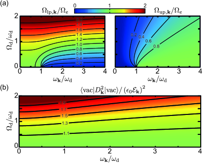
Figure 2: (a) Colorplot of the polariton-vacuum Rabi frequencies as a function of the photon mode frequency $\omega_{\textbf{k}}$ and of the dresser Rabi frequency $\Omega_{\rm d}$, for an emitter resonant with the lower ($\omega_{e}=\omega_{{\rm lp},\textbf{k}}$, left panel) or upper ($\omega_{e}=\omega_{{\rm up},\textbf{k}}$, right panel) polariton. (b) Colorplot of the vacuum fluctuations of the displacement field in the TM₀ mode.

In formal terms, we can rewrite the total Hamiltonian of Eq. (1) in the polariton basis as

$$H \approx\hbar\omega_{e}\sum_{\textbf{k}}b_{\textbf{k}}^{{\dagger}}b_{\textbf{k}}+$$ (3)

$$\quad+\sum_{\textbf{k}}\hbar\omega_{\text{up},\textbf{k}}p_{\text{up},\textbf{k}}^{{\dagger}}p_{\text{up},\textbf{k}}+\sum_{\textbf{k}}\hbar\omega_{\text{lp},\textbf{k}}p_{\text{lp},\textbf{k}}^{{\dagger}}p_{\text{lp},\textbf{k}}+$$

$$\quad+i\sum_{\textbf{k}}\left(\frac{\hbar\Omega_{\text{up},\textbf{k}}}{2}p_{\text{up},\textbf{k}}b_{\textbf{k}}^{{\dagger}}+\frac{\hbar\Omega_{\text{lp},\textbf{k}}}{2}p_{\text{lp},\textbf{k}}b_{\textbf{k}}^{{\dagger}}\right)+\text{h.c.},$$

where $p_{\,{\rm up},\textbf{k}},p_{\,{\rm lp},\textbf{k}}$ are the annihilation operators of a cavity-dresser polariton in the upper or lower polariton branches of (2) with eigenfrequencies

$$\omega_{{\rm up/lp},\textbf{k}}^{2}=\frac{\omega^{2}_{\textbf{k}}+\bar{\omega}_{\rm d}^{2}}{2}\pm\sqrt{\frac{\left(\bar{\omega}_{\rm d}^{2}-\omega^{2}_{\textbf{k}}\right)^{2}}{4}+\Omega_{\rm d}^{2}\omega^{2}_{\textbf{k}}}.$$ (4)

where $\bar{\omega}_{\rm d}=\sqrt{\omega^{2}_{\rm d}+\Omega^{2}_{\rm d}}$ includes the depolarization shift of the dresser frequency Załużny (1982); Ando et al. (1982); Cominotti et al. (2023). The effective polariton-vacuum Rabi frequencies quantifying the coupling strength between the emitter and the lower/upper cavity-dresser polaritons read (Secs.III and IV of the SM)

$$\frac{\Omega_{{\rm up},\textbf{k}}}{\Omega_{e}}=\sqrt{\frac{\omega^{2}_{\textbf{k}}}{\omega_{e}\omega_{{\rm up},\textbf{k}}}}\sin\theta_{\textbf{k}}\textrm{~{},~{}~{}}\frac{\Omega_{{\rm lp},\textbf{k}}}{\Omega_{e}}=\sqrt{\frac{\omega^{2}_{\textbf{k}}}{\omega_{e}\omega_{{\rm lp},\textbf{k}}}}\cos\theta_{\textbf{k}}\,,$$ (5)

with

$$\cos^{2}\theta_{\textbf{k}}=\frac{\omega_{{\rm up},\textbf{k}}^{2}-\omega_{\textbf{k}}^{2}}{\omega_{{\rm up},\textbf{k}}^{2}-\omega_{{\rm lp},\textbf{k}}^{2}}\textrm{~{},~{}~{}}\sin^{2}\theta_{\textbf{k}}=\frac{\omega_{\textbf{k}}^{2}-\omega_{{\rm lp},\textbf{k}}^{2}}{\omega_{{\rm up},\textbf{k}}^{2}-\omega_{{\rm lp},\textbf{k}}^{2}}.$$ (6)

Interestingly, all the information regarding the hybridization between the cavity photon and the dresser excitations due to the USC is contained in the hybridization angle $\theta_{\textbf{k}}$, which summarizes into a single parameter the Hopfield coefficients expressing the polariton operators $p_{\text{lp},\textbf{k}}$ and $p_{\text{up},\textbf{k}}$ in terms of the cavity photon $a_{\textbf{k}}$ and dresser $d_{\textbf{k}}$ operators and their hermitian conjugates Ciuti et al. (2005); De Liberato (2017).

The reformulation in terms of the polariton Hamiltonian (3) provides a physical understanding of the peculiar features displayed by the emitter-polariton coupling that have have observed in Fig.1(b). In Fig. 2(a) we show a color plot of the polariton-vacuum Rabi frequencies $\Omega_{{\rm lp},\textbf{k}}$ and $\Omega_{{\rm up},\textbf{k}}$ as a function of the wavenumber k and of the dresser Rabi frequency $\Omega_{\rm d}$, when the emitter is resonant with some state on the lower $\omega_{e}=\omega_{{\rm lp},\textbf{k}}$ (left panel) or the upper $\omega_{e}=\omega_{{\rm up},\textbf{k}}$ (right panel) polariton branch. In the full polariton spectrum of Fig.1(b), $\Omega_{{\rm lp/up},\textbf{k}}$ quantifies the magnitude of the Rabi splitting.

For a weak dresser Rabi frequency $\Omega_{\rm d}\ll\omega_{\rm d}$, the resonant lower and upper polariton-vacuum Rabi frequencies display similar behavior, with $\Omega_{{\rm lp(up)},\textbf{k}}\simeq\Omega_{e}$ when the polariton has a fully photonic nature and $\Omega_{{\rm up(lp)},\textbf{k}}\simeq 0$ when the polariton has a fully excitonic nature. In general, while the photonic weight is redistributed between the upper and lower polariton, the total weight is conserved, $\Omega_{{\rm lp},\textbf{k}}^{2}+\Omega_{{\rm up},\textbf{k}}^{2}\approx\Omega_{e}^{2}$, as a consequence of the weakly dressed regime where $\omega_{{\rm up/lp},\textbf{k}}\simeq\omega_{\textbf{k}}$.

The physics drastically changes when the dresser enters the USC regime for $\Omega_{\rm d}\simeq\omega_{\rm d}$. Here $\omega_{{\rm up/lp},\textbf{k}}\neq\omega_{\textbf{k}}$, and the square-root prefactors in (5) start to matter: the coupling with the lower polariton $\Omega_{{\rm lp},\textbf{k}}$ is reinforced and remains significant up to higher wavenumbers, while the upper polariton’s coupling $\Omega_{{\rm up},\textbf{k}}$ is significantly reduced. As an immediate consequence the conservation of the photonic weight is strongly violated, $\Omega_{{\rm lp},\textbf{k}}^{2}+\Omega_{{\rm up},\textbf{k}}^{2}\neq\Omega_{e}^{2}$. This quite remarkable behavior is due to the mixing of creation and annihilation operators in the Bogoliubov transformation to polariton operators Ciuti et al. (2005), so that the normal and anomalous terms constructively (destructively) interfere in determining the coupling of the lower (upper) polariton to the emitter.

This marked asymmetry of the Rabi splitting of the lower and upper polariton branches is straightforwardly observed in a cavity transmission/reflection spectroscopy experiment. Fig.3 displays examples of simulated transmission spectra well in the strong emitter-polariton coupling regime $\Omega_{\rm lp/up,\textbf{k}}\gg\gamma_{\rm lp/up}$ where all polariton branches are well separated.

Quantum fluctuations in the USC vacuum — In order to obtain a deeper understanding of the relation between the modified emitter light-matter coupling strength and the properties of the USC dressed vacuum, we evaluate the fluctuations of the cavity electric displacement field $D_{\textbf{k}}=i\sqrt{\epsilon_{0}\hbar\omega_{\textbf{k}}/(2SL_{c})}(a_{\textbf{k}}-a_{-\textbf{k}}^{{\dagger}})$. Within our dipole representation, this field -rather than the electric field- represents in fact the correct electromagnetic degree of freedom to describe light-matter interactions Cohen-Tannoudji et al. (1989); Craig and Thirunamachandran (1998); Stengel et al. (2009). By using the hybridization angle $\theta_{\textbf{k}}$ defined above, we can express this quantity as (Sec.V of the SM)

$$\frac{\langle{\rm vac}|D^{2}_{\textbf{k}}|{\rm vac}\rangle}{(\epsilon_{0}\mathcal{E}_{\textbf{k}})^{2}}=\frac{\omega_{\textbf{k}}}{\omega_{\rm up,\textbf{k}}}\sin^{2}\theta_{\textbf{k}}+\frac{\omega_{\textbf{k}}}{\omega_{\rm lp,\textbf{k}}}\cos^{2}\theta_{\textbf{k}}\\ =\frac{\omega_{e}}{\omega_{\textbf{k}}}\left(\frac{\Omega_{\rm lp,\textbf{k}}^{2}}{\Omega_{e}^{2}}+\frac{\Omega_{\rm up,\textbf{k}}^{2}}{\Omega_{e}^{2}}\right),$$ (7)

where $\mathcal{E}_{\textbf{k}}^{2}=(\hbar\omega_{\textbf{k}})/(2\epsilon_{0}SL_{c})$ are the quantum fluctuations of the electric (or, in this case equivalently, of the displacement) field in a bare cavity. The peculiarity of the USC is then visible in Fig. 2(b), where we display a color plot of the total electric displacement fluctuations in the different k modes as a function of the strength of the cavity dresser coupling $\Omega_{d}$.

On the one hand, for weak or moderate $\Omega_{d}$, the prefactors $\omega_{\textbf{k}}/\omega_{\{\textrm{up,lp}\},\textbf{k}}$ on the first line in Eq. (7) are close to one and thus play a minor role; thanks to the trigonometric identity $\sin^{2}\theta_{\textbf{k}}+\cos^{2}\theta_{\textbf{k}}=1$ associated to the conservation of the photonic weight, the two contributions then sum up to the standard bare vacuum fluctuations. On the other hand, the total fluctuations get substantially increased in the USC regime, in connection with the increased value of the lower polariton-vacuum Rabi frequencies. More in specific, the second line of (7) shows that the contributions of the lower and upper polariton frequencies to the vacuum fluctuations have an amplitude proportional to the polariton-emitter Rabi frequencies $\Omega_{\rm lp/up,\textbf{k}}$, a result that extends to the USC vacuum case the traditional concept of vacuum-field Rabi splitting Sanchez-Mondragon et al. (1983); Agarwal (1984).

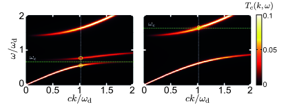
Figure 3: Colorplot of the transmission spectrum as a function of the incident wavevector k and frequency $\omega$. The white dashed line marks the wavevector location of the emitter minimal anticrossing, the green dashed line marks the emitter frequency $\omega_{e}$. The two yellow circles mark the locations where the polariton maximally hybridizes with the emitter. As in the previous figures, the left/right panels correspond to an emitter on resonance with the lower/upper polariton. Parameters: $\Omega_{e}/\omega_{\rm d}=0.2$, $\Omega_{\rm d}/\omega_{\rm d}=1$, $\omega_{e}/\omega_{\rm d}=0.7$ (left panel) and $1.6$ (right panel). The photonic, dresser and emitter decay rates are $\gamma/\omega_{\rm d}=0.01$, $\kappa_{\rm d}=\kappa_{e}=0.05\,\omega_{\rm d}$.

Spontaneous emission — While the Rabi splitting in the strong emitter-polariton coupling regime provides a most direct experimental signature of the modified Rabi couplings (5), a related effect is visible also in the spontaneous emission rate in the weak emitter-polariton coupling regime $\gamma_{\rm lp/up}\gg\Omega_{\rm lp/up,\textbf{k}}$ where the Rabi oscillations are replaced by an irreversible emission process. In our system, the spontaneous emission is mediated by the resonant polariton mode and its rate reads Purcell et al. (1946) $\Gamma_{\rm lp/up,\textbf{k}}\approx{\Omega_{\rm lp/up,\textbf{k}}^{2}}/{\gamma_{\rm lp,up}}$: in analogy with the corresponding modification of the Rabi splitting in the strong coupling regime, the effect of the USC vacuum state in the weak emitter-polariton coupling regime will be to reinforce (suppress) the spontaneous emission into the lower (upper) polariton by an amount related to the modified quantum fluctuations of the electric displacement field (7). In physical terms, this prediction can be understood as a novel form of the Purcell effect Purcell et al. (1946); Englund et al. (2005), where one acts on the modification of the overall intensity of the field fluctuations in the USC vacuum rather than on just their frequency redistribution. Interestingly, our result is in line with the theory of spontaneous emission in dielectric media, and has the key advantage of a clear disentanglement of local field effects Glauber and Lewenstein (1991); Knoester and Mukamel (1989); Scheel et al. (1999); Barnett et al. (1992); Berman and Milonni (2004); de Vries and Lagendijk (1998)

Discussion — Our previous derivations were carried out within a quantum language, so the modifications of the vacuum-field Rabi splitting and of the spontaneous emission rate were naturally related to the ones of the zero-point fluctuations (7). In connection to the intense debate that took place on the physical origin of spontaneous emission in terms of quantum fluctuation and/or radiative reaction effects Senitzky (1973); Milonni et al. (1973); Dalibard et al. (1982), it is interesting to assess whether our predictions can be equivalently expressed in classical terms of radiative reaction by the dressed electromagnetic field in the USC device.

As a first step in this direction, it is straightforward to notice that our theory can be directly reformulated in terms of motion equations for the cavity $a_{\textbf{k}}$ and the emitter $b_{\textbf{k}}$ and dresser $d_{\textbf{k}}$ polarization fields stemming from the Hamiltonian (1) and re-interpreted as classical variables. This set of equations can be summarized in a dispersion relation that can equivalently derived directly from Maxwell equations (Secs.VI-VIII of the SM) of the form $\omega^{2}\,\epsilon_{r}(\omega)=c^{2}k^{2}$, with the effective dielectric permittivity

$$\epsilon_{r}(\omega)=\frac{1}{1-\frac{\Omega_{d}^{2}}{\bar{\omega}_{d}^{2}-\omega^{2}-i\kappa_{\rm d}\omega}-\frac{\Omega_{e}^{2}}{\bar{\omega}_{e}^{2}-\omega^{2}-i\kappa_{e}\omega}}\,,$$ (8)

that is an analog of the Clausius-Mossotti formula in a multiple slab geometry Hopfield (1958); Böttcher et al. (1974) (here $\kappa_{\rm d},\kappa_{e}$ represent the dresser and emitter radiative losses, as already introduced in Fig. 3). Interestingly, the deviation of this expression from a naive simple sum of the individual slabs’ permittivities, $\epsilon_{r}(\omega)\approx 1+\Omega_{\rm d}^{2}/(\bar{\omega}_{\rm d}^{2}-\omega^{2}-i\kappa_{\rm d}\omega)+\Omega_{e}^{2}/(\bar{\omega}_{e}^{2}-\omega^{2}-i\kappa_{e}\omega)$ provides a signature of the key role played by the electrostatic interaction between the emitter and the dresser noticed in De Bernardis et al. (2018); Amelio et al. (2021); Sáez-Blázquez et al. (2023); Pantazopoulos et al. (2023), whose strength is indeed proportional to the product of the electron densities $n_{d}n_{e}\sim\Omega^{2}_{d}\Omega_{e}^{2}$. Once again, $\bar{\omega}^{2}_{d,e}={\omega}^{2}_{d,e}+\Omega_{d,e}^{2}$ are the depolarization-shifted values of the dresser and emitter frequencies Załużny (1982); Ando et al. (1982); Cominotti et al. (2023).

This formulation in terms of classical equations of motion is the strong emitter-polariton coupling generalization of the radiative reaction equations Senitzky (1973); Dalibard et al. (1982) in the case of a resonantly peaked density of states of the electromagnetic modes. The analogy to the radiative reaction equations is even closer in the weak emitter-polariton coupling regime: close to resonance to the lower (upper) polariton mode, integrating out the polariton field leads to a radiative damping term of the usual form (Sec. VIII of the SM) $\dot{b}_{\textbf{k}}=-i\omega_{e}b_{\textbf{k}}-\Omega_{\rm lp(up),\textbf{k}}^{2}/(2\gamma_{\rm lp(up)})\,b_{\textbf{k}}\,$. Physically, this close correspondence between the radiative reaction and the quantum fluctuations is a direct manifestation of the fluctuation-dissipation theorem relating the quantum fluctuations of the dressed polariton field in its vacuum state and the susceptibility of vacuum to the polarization of the emitter Barnett et al. (1992); Dalibard et al. (1982). All together, these arguments show how the whole vacuum phenomenology described so far can be equivalently re-interpreted in terms of electrodynamics in dense dielectric media.

Conclusions and outlook — In this work, we have theoretically investigated how basic light-matter interaction processes are modified in the distorted vacuum state of a semiconductor-based cavity QED system in the ultra-strong coupling (USC) regime. In particular, we have focused our attention on quantities of direct experimental access such as the vacuum-field Rabi splitting of an additional emitter strongly coupled to USC polaritons, and its spontaneous emission in the weak emitter-polariton coupling limit. In both cases, a signature of the distorted vacuum state of the USC regime is visible as a marked asymmetry between the polariton branches.

Even though our discussion is focused on a specific material system of major experimental interest, the predicted effects generally apply to any optical system in the USC regime. As such, our conclusions are of interest for a broad community of researchers, from circuit-QED devices, to semiconductor optoelectronics and terahertz optics and validate the picture that engineering the QED vacuum is indeed a powerful tool to control optical processes and, on the longer run, possibly also manipulate the properties of materials Garcia-Vidal et al. (2021); Bloch et al. (2022); Andolina et al. (2022).

From a conceptual standpoint, we have shown that our predictions can be equivalently understood in terms of classical radiative reaction in dielectric materials or in terms of quantum fluctuations in the distorted USC vacuum state, the two pictures being connected by the fluctuation-dissipation theorem. On one hand, the connection to classical radiative reaction provides a new point of view on vacuum effects as a tool to control materials, a concept that is attracting a growing interest, but is typically investigated within a quantum language Ashida et al. (2020, 2023); Arwas and Ciuti (2023); Curtis et al. (2023); Garcia-Vidal et al. (2021); Bloch et al. (2022). On the other hand, the quantum picture provides a transparent framework to go beyond a Fermi golden rule analysis of spontaneous emission in dielectric materials and describe the interplay of ultra-strong coupling with more sophisticated light-matter interaction phenomena such as parametric downconversion, which directly involve the amplification of quantum fluctuations.

Supplementary material for:
Modification of light-matter interactions in the vacuum of ultrastrongly coupled systems

Daniele De Bernardis^1,2, Gian Marcello Andolina², and Iacopo Carusotto¹

I Intersubband polaritons in the dipole representation

We review here the details of the derivation of the intersubband (ISB) polariton Hamiltonian valid in the ultrastrong coupling (USC) regime, based on Ref. Todorov and Sirtori (2012). Initially we focus only on a single quantum well (QW) and in the next section we generalize it to a multi-well configuration.

The polarization density can be written explicitly in terms of raising/lowering operators of the respective intersubband transition Todorov and Sirtori (2012)

$$\textbf{P}(\textbf{r})=\frac{e}{S}\sum_{\mu>\nu,\textbf{k}}\zeta_{\mu\nu}(z)e^{i\textbf{k}\cdot\textbf{r}_{\parallel}}\left(B_{\mu\nu\textbf{k}}+B_{\mu\nu-\textbf{k}}^{{\dagger}}\right)\textbf{u}_{z},$$ (S1)

Here $e$ is the electron charge, $S$ is the surface area of the slab (assumed to be equal to the cavity) and $\textbf{u}_{z}$ is a unit vector along the $z$-axis. The in-plane position is $\textbf{r}_{\parallel}=(x,y,0)$ and $\textbf{k}=(k_{x},k_{y},0)$ is the in-plane wavector. The dipole density is given by

$$\zeta_{\mu\nu}(z)=z\psi_{\mu}^{*}(z)\psi_{\nu}(z).$$ (S2)

Here $\psi_{\mu}(z)$ is the wavefunction of the $\mu$-th level of the QW Todorov and Sirtori (2012); Todorov (2015, 2014), defined in the interval $[z_{\rm qw}-L_{\rm qw}/2,z_{\rm qw}+L_{\rm qw}/2]$, where $L_{\rm qw}$ is the size of the quantum well along the $z$-axis and $z_{\rm qw}$ is its central position. The ISB transition operators are given by

$$B_{\mu\nu\textbf{k}}=\sum_{\textbf{q}}\tilde{\Psi}^{{\dagger}}_{\nu,\textbf{q}-\textbf{k}}\tilde{\Psi}_{\mu,\textbf{q}},$$ (S3)

where $\tilde{\Psi}_{\mu,\textbf{k}}$ is the Fermionic operator that annihilates an electron with in-plane momentum k in the $\mu$-th subband. It is convenient to rewrite this operator as

$$B_{\mu\nu\textbf{k}}=\sqrt{N_{\mu\nu}}b_{\mu\nu\textbf{k}}.$$ (S4)

where $N_{\mu\nu}=\braket{\hat{N}_{\nu}}-\braket{\hat{N}_{\mu}}$ is the electron population imbalance between two subbands. Considering only low energy transitions which take place just from the ground state (Fermi sea) to an upper band and assuming $N_{\mu\nu}\gg 1$ (heavy doping), we have that

$$[b_{\mu\nu\textbf{k}},b_{\mu^{\prime}\nu^{\prime}\textbf{k}\,^{\prime}}^{{\dagger}}]\simeq\delta_{\mu\mu^{\prime}}\delta_{\nu\nu^{\prime}}\delta_{\textbf{k}\,\textbf{k}\,^{\prime}}$$ (S5)

and the transition operators behave as Bosonic creation/annihilation operators for the collective excitation. Considering only transitions from the lowest subband, in the low excitation limit, we have that $N_{\mu\nu=0}\approx N$, where $N$ is the total number of electrons. From now on we always consider only transitions from the lowest subband, suppressing the index $\nu$. The QW Hamiltonian is then just given by a collection of harmonic oscillators

$$H_{\rm qw}=\hbar\omega_{\rm qw}\sum_{\textbf{k}}b_{\textbf{k}}^{{\dagger}}b_{\textbf{k}}.$$ (S6)

The light-matter Hamiltonian for the QW coupled to the cavity field can be derived by considering the total energy of the system, which is given by the matter’s energy plus the electromagnetic energy Jackson (1999)

$$\begin{split}H&=H_{\rm qw}+H_{\rm em}\\ &=H_{\rm qw}+\int d^{3}r\left[\frac{\textbf{E}^{2}(\textbf{r})}{2\epsilon_{0}}+\frac{\epsilon_{0}c^{2}}{2}\textbf{B}^{2}(\textbf{r})\right].\end{split}$$ (S7)

The coupling between matter and the electromagnetic field is provided by the fact that the charged matter generates and changes the electric and magnetic field. In the so-called dipole gauge this is realized by the following minimal coupling substitution in the cavity electric field energy density Jackson (1999)

$$\epsilon_{0}\textbf{E}(\textbf{r})=\textbf{D}(\textbf{r})-\textbf{P}(\textbf{r}).$$ (S8)

Notice that here we take only the displacement field to be transverse Cohen-Tannoudji et al. (1989), such that $\vec{\nabla}\cdot\textbf{D}(\textbf{r})=0$. In this way we correctly recover Maxwell equations with a polarizable medium, where $\vec{\nabla}\cdot\textbf{E}(\textbf{r})=-\vec{\nabla}\cdot\textbf{P}(\textbf{r})/\epsilon_{0}=\rho_{b}(\textbf{r})/\epsilon_{0}$, where $\rho_{b}(\textbf{r})$ is the so-called bound charge density Jackson (1999).

The total light-matter Hamiltonian is then given by Cohen-Tannoudji et al. (1989)

$$\begin{split}H=H_{\rm qw}+\int d^{3}r\left[\frac{\left(\textbf{D}(\textbf{r})-\textbf{P}(\textbf{r})\right)^{2}}{2\epsilon_{0}}-\frac{\epsilon_{0}c^{2}}{2}\textbf{A}(\textbf{r})\cdot\nabla^{2}\textbf{A}(\textbf{r})\right].\end{split}$$ (S9)

The electric displacement in the cavity made of two perfect parallel mirrors can be written as Jackson (1999); Sáez-Blázquez et al. (2023)

$$\begin{split}\textbf{D}(\textbf{r})=i\sum_{n,\textbf{k},\sigma}\sqrt{\frac{\epsilon_{0}\hbar\omega_{n,\textbf{k}}}{2}}\Bigg{[}\textbf{w}_{n,\textbf{k}}^{\sigma}(\textbf{r}_{\parallel},z)a_{n,\textbf{k}}-\left(\textbf{w}_{n,\textbf{k}}^{\sigma}(\textbf{r}_{\parallel},z)\right)^{*}a_{n,-\textbf{k}}^{{\dagger}}\Bigg{]}.\end{split}$$ (S10)

Here the cavity mode functions are solutions of the Poisson equation and can be written as Sáez-Blázquez et al. (2023)

$$\textbf{w}_{n,\textbf{k}}^{\sigma}(\textbf{r}_{\parallel},z)=\frac{e^{i\textbf{k}\cdot\textbf{r}_{\parallel}}}{\sqrt{S}}\sqrt{\frac{2}{L_{c}\left(1+\delta_{n,0}\right)}}\begin{pmatrix}i\varepsilon^{(x)}_{n,\textbf{k},\sigma}\sin(k_{n}z)\\ i\varepsilon^{(y)}_{n,\textbf{k},\sigma}\sin(k_{n}z)\\ \varepsilon^{(z)}_{n,\textbf{k},\sigma}\cos(k_{n}z)\\ \end{pmatrix},$$ (S11)

where $S=L_{x}L_{y}$ is the surface area of the rectangular cavity $L_{c}$ is the cavity height, and $k_{n}=\pi/L_{c}n$, with $n=0,1,2\ldots$ is the wavevector along the cavity axis, where metallic boundary conditions are assumed. The index $\sigma=1,2$ is the polarization index.

Considering only ISB transitions from the lowest subband, the interaction light-matter Hamiltonian for a single QW placed at $z=z_{\rm qw}$ is

$$\begin{split}H_{I}&=\int d^{3}r\frac{1}{\epsilon_{0}}\left[-\textbf{D}\cdot\textbf{P}+\frac{P^{2}}{2}\right]\\ &=-i\frac{\hbar\omega_{P}}{2}\sum_{n,\textbf{k},\sigma,\mu}\varepsilon^{(z)}_{n,\textbf{k},\sigma}\sqrt{f^{n}_{\mu 0}\frac{\omega_{n,\textbf{k}}}{\omega_{\mu 0}}}(a_{n,\textbf{k}}-a_{n,-\textbf{k}}^{{\dagger}})\left(b_{\mu-\textbf{k}}+b_{\mu\textbf{k}}^{{\dagger}}\right)\\ &+\frac{\hbar\omega_{P}^{2}}{4}\sum_{\textbf{k}}\sum_{\mu,\mu^{\prime}}\frac{I_{\mu\mu^{\prime}}}{\sqrt{\omega_{\mu 0}\omega_{\mu^{\prime}0}}}\left(b_{\mu\textbf{k}}+b_{\mu-\textbf{k}}^{{\dagger}}\right)\left(b_{\mu^{\prime}\textbf{k}}+b_{\mu^{\prime}-\textbf{k}}^{{\dagger}}\right)\end{split}$$ (S12)

Here the main coupling parameter is the plasma frequency

$$\omega_{P}^{2}=\frac{Ne^{2}}{\epsilon_{0}mSL_{c}},$$ (S13)

and $m$ is the electron effective mass. The generalized oscillator strength is defined as

$$\begin{split}f^{n}_{\mu 0}=\frac{2m\omega_{\mu 0}}{\hbar}\frac{2}{1+\delta_{n0}}\left[\int_{-\infty}^{\infty}dz\zeta_{\mu 0}(z)\cos\left(k_{n}z\right)\right]^{2}.\end{split}$$ (S14)

For $n=0$ it coincides with the usual oscillator strength of the $\mu$-th dipole transition $f_{\mu 0}=2m\omega_{\mu 0}z_{\mu 0}^{2}/\hbar$, where

$$z_{\mu 0}=\braket{\mu}{z}{0}=\int_{-\infty}^{\infty}dz\zeta_{\mu 0}(z)$$ (S15)

is the ISB dipole matrix element. At higher $n>0$, it also contains all the multipoles matrix elements, as it has to be by interacting with a non-homogeneous electric field. The higher the $n$-th mode is the more multipolar will be the ISB excitation.

In the last term of Eq. (S12) we introduced the $P^{2}$-interaction tensor strength

$$\begin{split}I_{\mu\mu^{\prime}}&=\frac{4m^{2}L_{c}}{\hbar^{2}}\omega_{\mu 0}\omega_{\mu^{\prime}0}\int_{-\infty}^{\infty}dz\zeta_{\mu 0}(z)\zeta_{\mu^{\prime}0}(z)\\ &=\frac{4m^{2}L_{c}}{\hbar^{2}}\omega_{\mu 0}\omega_{\mu^{\prime}0}\int_{-\infty}^{\infty}dzdz^{\prime}\delta(z-z^{\prime})\zeta_{\mu 0}(z)\zeta_{\mu^{\prime}0}(z^{\prime})\\ &=\frac{4m^{2}L_{c}}{\hbar^{2}}\omega_{\mu 0}\omega_{\mu^{\prime}0}\sum_{n=0}\int_{-\infty}^{\infty}dz\zeta_{\mu 0}(z)\chi_{n}(z)\times\int_{-\infty}^{\infty}dz\zeta_{\mu^{\prime}0}(z)\chi_{n}(z),\end{split}$$ (S16)

where in the last equality we introduced a complete basis such that $\sum_{n=0}\chi_{n}(z)\chi_{n}(z^{\prime})=\delta(z-z^{\prime})$.

Truncating the ISB transitions to $\mu=1$ only, we suppress also the index $\mu$ having $b_{\mu,\textbf{k}}\mapsto b_{\textbf{k}}$ and defining $\omega_{\rm qw}=\omega_{10}$ and $f^{n}_{\rm qw}=f^{n}_{10}$. The interaction Hamiltonian becomes

$$\begin{split}H_{I}\approx-i\frac{\hbar\omega_{P}}{2}\sum_{n,\textbf{k},\sigma}\varepsilon^{(z)}_{n,\textbf{k},\sigma}\sqrt{f^{n}_{\rm qw}\frac{\omega_{n,\textbf{k}}}{\omega_{\rm qw}}}(a_{n,\textbf{k}}-a_{n,-\textbf{k}}^{{\dagger}})\left(b_{-\textbf{k}}+b_{\textbf{k}}^{{\dagger}}\right)+\frac{\hbar\omega_{P}^{2}}{4\omega_{\rm qw}}\sum_{\textbf{k},n}f_{\rm qw}^{n}\left(b_{\textbf{k}}+b_{-\textbf{k}}^{{\dagger}}\right)\left(b_{\textbf{k}}+b_{-\textbf{k}}^{{\dagger}}\right)\end{split}$$ (S17)

where we have used $\chi_{n}(z)=\sqrt{2/(L_{c}(1+\delta_{n,0}))}\cos(k_{n}z)$ Todorov and Sirtori (2012).

The ISB transition couple mostly with the so-called TM₀ mode Todorov (2015), which corresponds to the $n=0$ mode, entirely polarized along the cavity axis ($z$-axis), with $\varepsilon^{(z)}_{0,\textbf{k},\sigma}=\delta_{z,\sigma}$. The light-matter Hamiltonian can be further simplified to

$$\begin{split}&H\approx\hbar\omega_{\rm qw}\sum_{\textbf{k}}b_{\textbf{k}}^{{\dagger}}b_{\textbf{k}}+\sum_{\textbf{k}}\hbar\omega_{\textbf{k}}a_{\textbf{k}}^{{\dagger}}a_{\textbf{k}}-i\frac{\hbar\omega_{P}}{2}\sum_{\textbf{k}}\sqrt{f_{\rm qw}\frac{\omega_{\textbf{k}}}{\omega_{\rm qw}}}(a_{\textbf{k}}-a_{-\textbf{k}}^{{\dagger}})\left(b_{-\textbf{k}}+b_{\textbf{k}}^{{\dagger}}\right)+\frac{\hbar\omega_{P}^{2}}{4\omega_{\rm qw}}\sum_{\textbf{k}}f_{\rm qw}\left(b_{\textbf{k}}+b_{-\textbf{k}}^{{\dagger}}\right)\left(b_{\textbf{k}}+b_{-\textbf{k}}^{{\dagger}}\right),\end{split}$$ (S18)

where we have suppressed the $n$ index everywhere. After all these passages we are left with an effective light-matter Hamiltonian describing the interaction with only the TM₀ cavity mode Todorov and Sirtori (2012), which can be rewritten as

$$\begin{split}H_{{\rm TM}_{0}}=H_{\rm qw}+L_{c}\int d^{2}r\left[\frac{\left(D(\textbf{r}_{\parallel})-P(\textbf{r}_{\parallel})\right)^{2}}{2\epsilon_{0}}-\frac{\epsilon_{0}c^{2}}{2}A(\textbf{r}_{\parallel})\nabla^{2}A(\textbf{r}_{\parallel})\right].\end{split}$$ (S19)

Here the displacement and the vector potential fields are scalar variables, meant to describe the $z$-component of the TM₀ modes, which are independent of the position along the $z$-axis (perpendicular to the cavity plane) and thus depends only from the in-plane position $\textbf{r}_{\parallel}$

$$D(\textbf{r}_{\parallel})=i\sum_{\textbf{k}}\sqrt{\frac{\epsilon_{0}\hbar\omega_{\textbf{k}}}{2SL_{c}}}e^{i\textbf{k}\cdot\textbf{r}_{\parallel}}(a_{\textbf{k}}-a_{-\textbf{k}}^{{\dagger}})$$ (S20)

$$A(\textbf{r}_{\parallel})=\sum_{\textbf{k}}\sqrt{\frac{\epsilon_{0}\hbar}{2SL_{c}\omega_{\textbf{k}}}}e^{i\textbf{k}\cdot\textbf{r}_{\parallel}}(a_{\textbf{k}}+a_{-\textbf{k}}^{{\dagger}}),$$ (S21)

with $[a_{\textbf{k}},a_{\textbf{k}\,^{\prime}}^{{\dagger}}]=\delta_{\textbf{k},\textbf{k}\,^{\prime}}$. The effective polarization density coupled to the TM₀ modes is also a scalar quantity, and is given by

$$P(\textbf{r}_{\parallel})=\frac{ez_{10}\sqrt{N}}{SL_{c}}\sum_{\textbf{k}}e^{i\textbf{k}\cdot\textbf{r}_{\parallel}}\left(b_{\textbf{k}}+b_{-\textbf{k}}^{{\dagger}}\right),$$ (S22)

It is worth noticing that nor the electromagnetic field densities nor the polarization densities of this TM₀-effective-description depends from the $z$-coordinate and so the overall physics does not depend from the position of the QW inside the cavity or its distance with respect to one or the other metallic plate. This is in principle in contradiction with basics electromagnetism, where any charge configuration between metallic plates would generates image charges which will affect its behaviour as a function of the distance from the plate De Bernardis et al. (2018). This contradiction emerges as a consequence of the truncation to the TM₀ mode only, for which we have discarded all the information regarding the presence of image charges and eventual Coulombic corrections. However we argue that this corrections are most often negligible for our specific aims.

II Polariton Hamiltonian for two stacked wells

Since the polarization of the matter inside the cavity is given by the sum over all its individual components, i.e. as a sum over all different quantum wells

$$\textbf{P}(\textbf{r})=\sum_{i=1}^{N_{\rm qw}}\textbf{P}_{i}(\textbf{r}),$$ (S23)

and each polarization do not overlap with the others $\int d^{3}r\textbf{P}_{i}(\textbf{r})\cdot\textbf{P}_{j}(\textbf{r})=0$ if $i\neq j$, we can easily generalize the Hamiltonian in Eq. (S19) to a multi-wells setup. Notice that this condition of non-overlapping polarization densities is exactly the condition of localized dipoles used in the standard applications of the dipole picture Cohen-Tannoudji et al. (1989). As a consequence the direct Coulomb interaction between different QWs disappears in favour of a fully local mediated interaction through the dynamical cavity field.

In the simplest case of two QWs, the dresser and emitter, as in the main text, the resulting Hamiltonian is

$$\begin{split}H=H_{\rm d}+H_{e}+L_{c}\int d^{2}r\left[\frac{D^{2}}{2\epsilon_{0}}-\frac{\epsilon_{0}c^{2}}{2}A\nabla^{2}A\right]+L_{c}\int d^{2}r\frac{1}{\epsilon_{0}}\left[-DP_{\rm d}+\frac{P_{\rm d}^{2}}{2}\right]+L_{c}\int d^{2}r\frac{1}{\epsilon_{0}}\left[-DP_{e}+\frac{P_{e}^{2}}{2}\right].\end{split}$$ (S24)

Since the two QWs have different electron number $N_{\rm d},N_{e}$, they also have different plasma frequencies. These can be cast into the two Rabi frequencies

$$\begin{split}&\Omega_{\rm d}^{2}=f_{\rm d}\frac{N_{\rm d}e^{2}}{\epsilon_{0}mSL_{c}},\\ &\Omega_{e}^{2}=f_{e}\frac{N_{e}e^{2}}{\epsilon_{0}mSL_{c}}.\end{split}$$ (S25)

Notice that here we are using all the definitions of Sec. I replacing all the subscripts ${\rm qw}\mapsto{\rm d},e$.

Introducing the creation-annihilation operators like in Sec. I, the total cavity QED Hamiltonian for the dresser and emitter QWs is thus given by

$$\begin{split}H=&\omega_{\rm d}\sum_{\textbf{k}}d_{\textbf{k}}^{{\dagger}}d_{\textbf{k}}+\omega_{e}\sum_{\textbf{k}}b_{\textbf{k}}^{{\dagger}}b_{\textbf{k}}+\sum_{\textbf{k}}\omega_{\textbf{k}}a^{{\dagger}}_{\textbf{k}}a_{\textbf{k}}\\ &-\frac{i\hbar\Omega_{\rm d}}{2}\sum_{\textbf{k}}\sqrt{\frac{\omega_{\textbf{k}}}{\omega_{\rm d}}}\left(a_{\textbf{k}}-a_{-\textbf{k}}^{{\dagger}}\right)\left(d_{-\textbf{k}}+d_{\textbf{k}}^{{\dagger}}\right)-\frac{i\hbar\Omega_{e}}{2}\sum_{\textbf{k}}\sqrt{\frac{\omega_{\textbf{k}}}{\omega_{e}}}\left(a_{\textbf{k}}-a_{-\textbf{k}}^{{\dagger}}\right)\left(b_{-\textbf{k}}+b_{\textbf{k}}^{{\dagger}}\right)\\ &+\frac{\hbar\omega_{{\rm d}}^{2}}{4\omega_{\rm d}}\sum_{\textbf{k}}\left(d_{-\textbf{k}}+d_{\textbf{k}}^{{\dagger}}\right)\left(d_{-\textbf{k}}+d_{\textbf{k}}^{{\dagger}}\right)+\frac{\hbar\omega_{{e}}^{2}}{4\omega_{e}}\sum_{\textbf{k}}\left(b_{-\textbf{k}}+b_{\textbf{k}}^{{\dagger}}\right)\left(b_{-\textbf{k}}+b_{\textbf{k}}^{{\dagger}}\right).\end{split}$$ (S26)

Assuming that the emitter polarization is always small, such that it never goes in the ultrastrong coupling regime we can neglect the $\sim P_{e}^{2}$-term of the emitter, which is the last term in Eq. (S26). In this way we recover the cavity-dresser-emitter Hamiltonian in the main text.

III Polaritons from canonical transformations

Here we consider the cavity-dresser Hamiltonian only defined in Eq. (S18) In this section we will suppress the vector notation for the in-plane wavevector $\textbf{k}\mapsto k$ in order to simplify the notation.

We then reintroduce the real canonical coordinates defining the quadrature operators

$$\begin{split}D_{k}&=-i\sqrt{\frac{\omega_{k}}{2}}\left(a_{k}-a^{{\dagger}}_{-k}\right),\\ A_{k}&=\frac{1}{\sqrt{2\omega_{k}}}\left(a_{k}+a^{{\dagger}}_{-k}\right),\\ \Pi_{k}&=-i\sqrt{\frac{\omega_{\rm d}}{2}}\left(d_{k}-d^{{\dagger}}_{-k}\right),\\ X_{k}&=\frac{1}{\sqrt{2\omega_{\rm d}}}\left(d_{k}+d^{{\dagger}}_{-k}\right).\\ \end{split}$$ (S27)

The cavity-dresser Hamiltonian becomes

$$\begin{split}&H_{c-{\rm d}}=\sum_{k}\left[\frac{\Pi_{k}^{2}}{2}+\frac{\omega_{\rm d}^{2}+\Omega_{\rm d}^{2}}{2}X_{k}^{2}\right]+\\ &+\sum_{k}\left[\frac{D_{k}^{2}}{2}+\frac{\omega_{k}^{2}}{2}A_{k}^{2}\right]+\sum_{k}\Omega_{\rm d}D_{k}X_{k}.\end{split}$$ (S28)

We make a canonical transformation (just a re-labelling)

$$\begin{split}\tilde{D}_{k}&=-\omega_{k}A_{k},\\ \tilde{A}_{k}&=\frac{1}{\omega_{k}}D_{k},\\ \end{split}$$ (S29)

We then have

$$\begin{split}&H_{c-{\rm d}}=\sum_{k}\left[\frac{\Pi_{k}^{2}}{2}+\frac{\omega_{\rm d}^{2}+\Omega_{\rm d}^{2}}{2}X_{k}^{2}\right]+\\ &+\sum_{k}\left[\frac{\tilde{D}_{k}^{2}}{2}+\frac{\omega_{k}^{2}}{2}\tilde{A}_{k}^{2}\right]+\sum_{k}\Omega_{\rm d}\omega_{k}\tilde{A}_{k}X_{k}.\end{split}$$ (S30)

The Hamiltonian in this form can be cast to a matrix, considering $H_{c-{\rm d}}=1/2v^{T}Mv$, where $v^{T}=(X_{k},\tilde{A}_{k},\Pi_{k},\tilde{D}_{k})$, and

$$M=\begin{pmatrix}\omega_{\rm d}^{2}+\Omega_{\rm d}^{2}&\Omega_{\rm d}\omega_{k}&0&0\\ \Omega_{\rm d}\omega_{k}&\omega_{k}^{2}&0&0\\ 0&0&1&0\\ 0&0&0&1\\ \end{pmatrix}$$ (S31)

Diagonalising $M$ is now equivalent to diagonalise the Hamiltonian. We can achieve this by considering the following unitary transformation

$$U=\begin{pmatrix}R&0_{2\times 2}\\ 0_{2\times 2}&R\\ \end{pmatrix}$$ (S32)

where $R$ is a $2\times 2$ rotation

$$R=\begin{pmatrix}\cos\theta&\sin\theta\\ -\sin\theta&\cos\theta\\ \end{pmatrix}$$ (S33)

In order to further simplify all the expressions we make implicit the dependence from the wavenumber $q$. Moreover we define

$$\begin{split}&\Omega_{X}=\omega_{\rm d}^{2}+\Omega_{\rm d}^{2}\\ &G=\Omega_{\rm d}\omega_{k}\\ &\Omega_{A}=\omega_{k}^{2}\\ \end{split}$$ (S34)

so

$$M=\begin{pmatrix}\Omega_{X}&G&0&0\\ G&\Omega_{A}&0&0\\ 0&0&1&0\\ 0&0&0&1\\ \end{pmatrix}$$ (S35)

We then find

$$\begin{split}\cos\theta&=\sqrt{\frac{1}{2}\left(1+\frac{\Omega_{X}-\Omega_{A}}{\sqrt{\left(\Omega_{X}-\Omega_{A}\right)^{2}+4G^{2}}}\right)}=\sqrt{\frac{\omega_{\rm up}^{2}-\omega_{k}^{2}}{\omega_{\rm up}^{2}-\omega_{\rm lp}^{2}}}\\ \sin\theta&=\sqrt{\frac{1}{2}\left(1-\frac{\Omega_{X}-\Omega_{A}}{\sqrt{\left(\Omega_{X}-\Omega_{A}\right)^{2}+4G^{2}}}\right)}=\sqrt{\frac{\omega_{k}^{2}-\omega_{\rm lp}^{2}}{\omega_{\rm up}^{2}-\omega_{\rm lp}^{2}}}\\ \end{split}$$ (S36)

with the diagonal matrix

$$M^{\prime}=\begin{pmatrix}\omega_{\rm up}^{2}&0&0&0\\ 0&\omega_{\rm lp}^{2}&0&0\\ 0&0&1&0\\ 0&0&0&1\\ \end{pmatrix}$$ (S37)

where

$$\omega_{\rm up/lp}^{2}=\frac{\Omega_{X}+\Omega_{A}}{2}\pm\frac{1}{2}\sqrt{\left(\Omega_{X}-\Omega_{A}\right)^{2}+4G^{2}}$$ (S38)

Working in the canonical representation has the convenience that, together with the eigenfrequencies, we have full access on the hybridization of the degrees of freedom due to the USC regime. Differently from previous works Frisk Kockum et al. (2019); Forn-Díaz et al. (2019), we can condense the full knowledge of the four Hopfield coefficients Hopfield (1958); Ciuti et al. (2005), in a single mixing angle $\theta_{k}$.

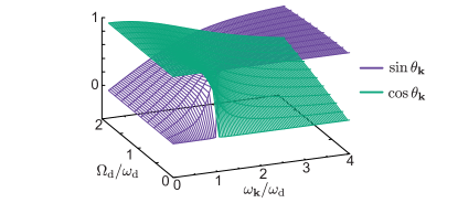
Figure S1: Canonical Hopfield coefficient $\sin\theta_{\textbf{k}},~{}\cos\theta_{\textbf{k}}$ as a function of the in-plane momentum and of the Rabi dressing $\Omega_{\rm d}$.

In Fig. S1 we show the behaviour of the canonical Hopfield coefficients as a function of the in-plane wavenumber $k$ and the dresser Rabi frequency $\Omega_{\rm d}$. When the dresser is only weakly doped, and $\Omega_{\rm d}\ll\omega_{\rm d}$ we observe a very small hybridization ($\cos\sim 1$ and $\sin\sim 0$ or vice versa), which become substantial only when the TM₀ is resonant with the dresser frequency at $ck=\omega_{\rm d}$ (and $\cos\sim\sin\sim 1/2$). On contrary, when the dresser is in the USC regime $\Omega_{\rm d}\simeq\omega_{\rm d}$, the light-matter hybridization becomes important on a large range of wavenumbers.

The USC Hamiltonian in the new diagonal variables looks like two uncoupled harmonic oscillators, representing the upper/lower polaritons

$$H_{c-{\rm d}}=\frac{\Lambda_{\rm up}^{2}}{2}+\frac{\omega_{\rm up}^{2}}{2}\xi_{\rm up}^{2}+\frac{\Lambda_{\rm lp}^{2}}{2}+\frac{\omega_{\rm lp}^{2}}{2}\xi_{\rm lp}^{2}$$ (S39)

where

$$\begin{pmatrix}\xi_{\rm up}\\ \xi_{\rm lp}\\ \Lambda_{\rm up}\\ \Lambda_{\rm lp}\\ \end{pmatrix}=U\begin{pmatrix}X\\ \tilde{A}\\ \Pi\\ \tilde{D}\\ \end{pmatrix}$$ (S40)

Evidently the eigenstates of Ham. (S39) are given by the polaritonic operators

$$p_{\rm up/lp}=\frac{1}{\sqrt{2\omega_{\rm up/lp}}}\Lambda_{\rm up/lp}-i\sqrt{\frac{\omega_{\rm up/lp}}{2}}\xi_{\rm up/lp}$$ (S41)

IV The polaritonic photon

For a moment we focus only on the cavity-dresser Hamiltonian. Using the canonical transformation diagonalization method explained in Appendix III we can rewrite the cavity-dresser plasma Hamiltonian as

$$\begin{split}&H_{c-{\rm d}}=\sum_{\textbf{k}}\left[\,\hbar\omega_{\rm lp,\textbf{k}}\,p_{\,{\rm lp},\textbf{k}}^{{\dagger}}p_{\,{\rm lp},\textbf{k}}\,+\,\hbar\omega_{\rm up,\textbf{k}}\,p_{\,{\rm up},\textbf{k}}^{{\dagger}}p_{\,{\rm up},\textbf{k}}\right]~{}.\end{split}$$ (S42)

Here $p_{\,{\rm lp},\textbf{k}}$ and $p_{\,{\rm up},\textbf{k}}$ represent the annihilation operators of the lower and upper polaritons, and their frequencies are given by (see Sec. III of the SM )

$$\omega_{\rm up/lp,\textbf{k}}^{2}=\frac{\omega^{2}_{\textbf{k}}+\omega_{\rm d}^{2}+\Omega_{\rm d}^{2}}{2}\pm\frac{1}{2}\sqrt{\left(\omega_{\rm d}^{2}+\Omega_{\rm d}^{2}-\omega^{2}_{\textbf{k}}\right)^{2}+4\Omega_{\rm d}^{2}\omega^{2}_{\textbf{k}}}.$$ (S43)

The new polaritonic variables represent the correct degrees of freedom to describe the cavity-dresser system, and consequently all the physical quantities must be rewritten in this basis. Since that the coupling between the cavity and the emitter is given by

$$H_{{\rm int},e-c}=-\frac{1}{\epsilon_{0}}\int d^{3}r\textbf{D}(\textbf{r})\cdot\textbf{P}_{e}(\textbf{r}),$$ (S44)

for our aims we mainly need to transform the cavity electric displacement field, which can be rewritten following Sec. III of the SM and using the transformation in Eq. (S40)

$$\begin{split}D(\textbf{r})=i\sqrt{\frac{\epsilon_{0}\hbar}{2SL_{c}}}\sum_{\textbf{k}}\omega_{\textbf{k}}\,e^{i\textbf{k}\cdot\textbf{r}_{\parallel}}\left(\frac{\sin\theta_{\textbf{k}}}{\sqrt{\omega_{\rm up,\textbf{k}}}}p_{\,{\rm up},\textbf{k}}+\frac{\cos\theta_{\textbf{k}}}{\sqrt{\omega_{\rm lp,\textbf{k}}}}p_{\,{\rm lp},\textbf{k}}\right)+{\rm h.c.}.\end{split}$$ (S45)

Using the expression for the emitter polarization given in the main text, and assuming that the emitter is weakly doped, we can perform the rotating-wave approximation (RWA) in the emitter-cavity interaction in Eq. (1). It is worth noticing that the RWA cannot be implemented in Eq. (1) by only discarding the terms $\sim\left(a_{\textbf{k}}b_{\textbf{k}}\right),~{}\left(a^{{\dagger}}_{-\textbf{k}}b^{{\dagger}}_{-\textbf{k}}\right)$, but it requires to switch on the polaritonic picture, and considering the electric field displacement given by Eq. (S45). This is very similar to what happens in the open driven/dissipative description of USC, where one has to switch to the polaritonic picture in order to identify the positive/negative frequencies operators that, coupling to the external bath, form the correct jump operator of the system De Liberato (2014); Frisk Kockum et al. (2019); De Bernardis (2023).

For the sake of completeness is also worth to calculate the dresser polarization in the polariton basis, that will be useful in the next sections. It reads

$$\begin{split}P_{\rm d}(\textbf{r})=\sqrt{\frac{\epsilon_{0}\hbar}{2SL_{c}}\frac{\Omega_{\rm d}^{2}}{\omega_{\rm d}}}\sum_{\textbf{k}}\,e^{i\textbf{k}\cdot\textbf{r}_{\parallel}}\left(\sqrt{\frac{\omega_{\rm up,\textbf{k}}}{\omega_{\rm d}}}\cos\theta_{\textbf{k}}p_{\,{\rm up},\textbf{k}}+\sqrt{\frac{\omega_{\rm lp,\textbf{k}}}{\omega_{\rm d}}}\sin\theta_{\textbf{k}}p_{\,{\rm lp},\textbf{k}}\right)+{\rm h.c.}\end{split}$$ (S46)

V Hybridization angle and vacuum observables

The interest in the hybridization angle $\theta_{k}$ is not only limited in understanding the cavity-dresser components of the polariton excitations, but it is also linked to the understanding on how the vacuum of quantum electrodynamics is modified by the presence of matter. Indeed, by using again the canonical formalism in Sec. III of the SM, we can compute the expectation value of any observable over the USC polaritonic vacuum $|\rm vac\rangle$, defined by

$$p_{{\rm up/lp},\textbf{k}}|\rm vac\rangle=0.$$ (S47)

Using Eqs. (S45)-(S46) we can calculate the vacuum fluctuations of the cavity electric field considering that

$$E_{\rm TM_{0}}(\textbf{r})=\frac{D(\textbf{r})-P_{\rm d}(\textbf{r})}{\epsilon_{0}}.$$ (S48)

We thus have that

$$\begin{split}\langle{\rm vac}|E_{\rm TM_{0},\textbf{k}}^{2}|{\rm vac}\rangle&=\frac{1}{\epsilon_{0}}\langle{\rm vac}|D^{2}_{\textbf{k}}|{\rm vac}\rangle+\langle{\rm vac}|P_{\rm d,\textbf{k}}^{2}|{\rm vac}\rangle\\ &=\mathcal{E}_{\textbf{k}}^{2}\Bigg{[}\frac{\omega_{\textbf{k}}}{\omega_{\rm up,\textbf{k}}}\sin^{2}\theta_{\textbf{k}}+\frac{\omega_{\textbf{k}}}{\omega_{\rm lp,\textbf{k}}}\cos^{2}\theta_{\textbf{k}}+\frac{\Omega_{\rm d}^{2}}{\omega_{\rm d}^{2}}\left(\frac{\omega_{\rm lp,\textbf{k}}}{\omega_{\textbf{k}}}\sin^{2}\theta_{\textbf{k}}+\frac{\omega_{\rm up,\textbf{k}}}{\omega_{\textbf{k}}}\cos^{2}\theta_{\textbf{k}}\right)\Bigg{]},\end{split}$$ (S49)

where $\mathcal{E}_{\textbf{k}}^{2}=(\hbar\omega_{\textbf{k}})/(2\epsilon_{0}SL_{c})$. We immediately notice from the last line of this formula that the electric field fluctuations take a large contribution from the fluctuations of the dresser polarization, which are given by the intrinsic fluctuations of matter. Moreover, after a few algebraic steps, we have that

$$\langle{\rm vac}|P_{\rm d,\textbf{k}}^{2}|{\rm vac}\rangle=\frac{\Omega_{\rm d}^{2}}{\omega_{\rm d}\omega_{\textbf{k}}}\langle{\rm vac}|D^{2}_{\textbf{k}}|{\rm vac}\rangle,$$ (S50)

from which we arrive to

$$\langle{\rm vac}|E_{\rm TM_{0},\textbf{k}}^{2}|{\rm vac}\rangle=\frac{1}{\epsilon_{0}}\left[1+\frac{\Omega_{\rm d}^{2}}{\omega_{\rm d}\omega_{\textbf{k}}}\right]\langle{\rm vac}|D^{2}_{\textbf{k}}|{\rm vac}\rangle.$$ (S51)

It is worth noticing that - being a gauge non-invariant quantity - the physical significance of the electric displacement is sometimes considered obscure and confusing Purcell (1965). However, we can see here that in the dipole picture, the electric displacement is directly related to the TM₀ electric field fluctuations and it thus realizes a good proxy to explore the USC modifications of the electric field fluctuations.

Another interesting example that we report for completeness is the cavity virtual photon population

$$\begin{split}N_{\rm ph,\textbf{k}}=\braket{{\rm vac}}{\,a_{\textbf{k}}^{{\dagger}}a_{\textbf{k}}\,}{{\rm vac}}=\frac{\sin^{2}\theta_{\textbf{k}}}{4\,\omega_{\textbf{k}}}\frac{\omega_{\rm up,\textbf{k}}^{2}+\omega_{\textbf{k}}^{2}}{\omega_{\rm up,\textbf{k}}}+\frac{\cos^{2}\theta_{\textbf{k}}}{4\,\omega_{\textbf{k}}}\frac{\omega_{\rm lp,\textbf{k}}^{2}+\omega_{\textbf{k}}^{2}}{\omega_{\rm lp,\textbf{k}}}-\frac{1}{2},\end{split}$$ (S52)

and the bare-dresser virtual excitation population

$$\begin{split}N_{\rm d,\textbf{k}}=\braket{{\rm vac}}{\,d_{\textbf{k}}^{{\dagger}}d_{\textbf{k}}\,}{{\rm vac}}=\frac{\sin^{2}\theta_{\textbf{k}}}{4\,\omega_{\rm d}}\frac{\omega_{\rm lp,\textbf{k}}^{2}+\omega_{\rm d}^{2}}{\omega_{\rm lp,\textbf{k}}}+\frac{\cos^{2}\theta_{\textbf{k}}}{4\,\omega_{\rm d}}\frac{\omega_{\rm up,\textbf{k}}^{2}+\omega_{\rm d}^{2}}{\omega_{\rm up,\textbf{k}}}-\frac{1}{2}.\end{split}$$ (S53)

For many years, these quantities were at the center of the discussions around polaritonic vacuum observables Ciuti et al. (2005); Liberato et al. (2007); De Liberato (2017). However, their individual relevance is now considered marginal, since their physical meaning explicitly depends from the chosen representation Pilar et al. (2020). They are important only when correlated with physical gauge invariant quantities. An example of gauge-invariant quantities is the differential zero point frequency of the system $\Delta\omega_{\rm ZP}$ Ciuti et al. (2005). This is obtained subtracting the bare total zero point frequency for vanishing light-matter coupling from the interacting one. Taking the vacuum expectation value of the cavity-dresser Hamiltonian in Eq. (2) we have that

$$\begin{split}\Delta\omega_{\rm ZP}=\frac{\omega_{\rm up,\textbf{k}}+\omega_{\rm lp,\textbf{k}}}{2}-\frac{\omega_{\textbf{k}}+\omega_{\rm d}}{2}=\omega_{\textbf{k}}N_{\rm ph,\textbf{k}}+\omega_{\rm d}N_{\rm d,\textbf{k}}+\Omega_{\rm d}N_{\rm int,\textbf{k}}.\end{split}$$ (S54)

Here the last term represents the interaction energy, defined by

$$\begin{split}N_{\rm int,\textbf{k}}=\quad\frac{i}{2}\sqrt{\frac{\omega_{\textbf{k}}}{\omega_{\text{d}}}}\langle{\rm vac}|\left(a_{\textbf{k}}^{{\dagger}}-a_{-\textbf{k}}^{\vphantom{{\dagger}}}\right)\left(d_{-\textbf{k}}^{\vphantom{{\dagger}}}+d_{\textbf{k}}^{{\dagger}}\right)|{\rm vac}\rangle+\langle{\rm vac}|\frac{\Omega_{\text{d}}}{4\omega_{\text{d}}}\left(d_{\textbf{k}}^{\vphantom{{\dagger}}}+d_{-\textbf{k}}^{{\dagger}}\right)\left(d_{\textbf{k}}^{\vphantom{{\dagger}}}+d_{-\textbf{k}}^{{\dagger}}\right)|{\rm vac}\rangle.\end{split}$$ (S55)

It is worth noticing that this term contains both the cavity-dresser interaction and the dresser self interaction, which is notoriously known as the $P^{2}$-term De Bernardis et al. (2018); Todorov and Sirtori (2012); Grießer et al. (2016); Bamba and Ogawa (2014); Schäfer et al. (2020), responsible of the so-called polariton gap.

Interestingly, for the resonant wavevector $\textbf{k}_{\rm res}$, such that $\omega_{\textbf{k}_{\rm res}}=\omega_{\rm d}$, the interaction energy exactly vanishes

$$N_{\rm int,\textbf{k}_{\rm res}}=0,$$ (S56)

because the positive dresser self interaction ($P^{2}$-term) exactly compensates the negative cavity-dresser contribution in Eq. (S55). As a consequence the differential zero point frequency is completely determined by the cavity and dresser virtual excitation, taking the simple expression

$$N_{\rm ph,\textbf{k}_{\rm res}}=N_{\rm d,\textbf{k}_{\rm res}}=\frac{1}{2}\left(\sqrt{1+\frac{\Omega_{\rm d}^{2}}{4\omega_{\rm d}^{2}}}-1\right).$$ (S57)

In this case the virtual photon number $N_{\rm ph,\textbf{k}_{\rm res}}$ represents the electromagnetic energy that can be released by an instantaneous suppression of the cavity-dresser coupling Ciuti et al. (2005).

VI Classical theory of transmission spectra

Here we derive the linear response theory following from our cavity-dresser-emitter system. We start by considering the total Hamiltonian given in Eq. (S26) and rewriting it using the quadrature canonical representation for the cavity, the dresser and the emitter degrees of freedom as given in Sec. III of the SM

$$H=\frac{1}{2}v^{T}M_{\rm tot}v,$$ (S58)

where $v^{T}=(X_{\rm d}(k),X_{e}(k),\tilde{A}_{k},\Pi_{\rm d}(k),\Pi_{e}(k),\tilde{D}_{k})$ is the array containing the canonical variables obtained generalising the definition in Eq. (S27) to the emitter, while the Hamiltonian matrix is given by

$$M_{\rm tot}=\begin{pmatrix}\omega_{\rm d}^{2}+\Omega_{\rm d}^{2}&0&\Omega_{\rm d}\omega_{k}&0&0&0\\ 0&\omega_{e}^{2}+\Omega_{e}^{2}&\Omega_{e}\omega_{k}&0&0&0\\ \Omega_{\rm d}\omega_{k}&\Omega_{e}\omega_{k}&\omega_{k}^{2}&0&0&0\\ 0&0&0&1&0&0\\ 0&0&0&0&1&0\\ 0&0&0&0&0&1\\ \end{pmatrix}$$ (S59)

From here we can write down the equation of motion of the system (using the Hamilton equations), which match the standard dielectric description from classical electromagnetism. In the frequency domain, the equation of motion read

$$\mathcal{M}_{k}(\omega)\cdot\begin{pmatrix}A_{k}\\ X_{\rm d}(k)\\ X_{e}(k)\\ \end{pmatrix}=0$$ (S60)

where the dynamical matrix is given by

$$\begin{split}&\mathcal{M}_{k}(\omega)=\\ &\begin{pmatrix}\omega_{k}^{2}-(\omega+i\gamma/2)^{2}&i\omega\Omega_{\rm d}&i\omega\Omega_{e}\\ -i\omega\Omega_{\rm d}&\omega_{\rm d}^{2}-(\omega+i\kappa_{\rm d}/2)^{2}&-\Omega_{\rm d}\Omega_{e}\\ -i\omega\Omega_{e}&-\Omega_{\rm d}\Omega_{e}&\omega_{e}^{2}-(\omega+i\kappa_{e}/2)^{2}\\ \end{pmatrix}\end{split}$$ (S61)

Notice that here we introduce the cavity, dresser and emitter losses $\gamma,\kappa_{\rm d},\kappa_{e}$ in a phenomenological way, just inserting a viscous damping in the equations. The cavity transmission reads Ciuti and Carusotto (2006); Liberato et al. (2007)

$$T_{c}(k,\omega)=\gamma\omega_{k}\left[\mathcal{M}^{-1}_{k}\right]_{00}.$$ (S62)

VII Details on the hybridization angle measurement protocol

Here we give a detailed description of the protocol to measure the cavity-dresser hybridization angle from the emitter-cavity-dresser spectrum.

We call $\bar{\omega}_{e+},\bar{\omega}_{e-}$ the frequencies measured from the cavity transmission at the minimal anticrossing between the emitter and the cavity-dresser polaritons, while $\bar{k}_{\rm x}$ is the wavevector realizing the minimal anticrossing (we will keep using the bar $\bar{\cdot}$ only for quantities which are directly measured from an eventual experiment, and distinguish them from quantities derived from the theory). We can measure $\bar{k}_{\rm x},\bar{\omega}_{e+},\bar{\omega}_{e-}$ directly from a transmission (reflection) experiment by only detecting the two peaks around the emitter frequency. Since $\bar{\omega}_{e\pm}\simeq\omega_{\rm up/lp}\pm\Omega_{\rm up/lp}$, the upper/lower polariton frequency resonant with the emitter is given by

$$\bar{\omega}_{\rm up/lp}=\frac{\bar{\omega}_{e+}+\bar{\omega}_{e-}}{2}.$$ (S63)

(Notice that the distinction between upper and lower polariton is also experimentally well defined since the two polaritons are separated by a gap, making them clearly distinguishable). The measured emitter-polariton Rabi splitting is then given by

$$\bar{\Omega}_{\rm up/lp}=\frac{\bar{\omega}_{e+}-\bar{\omega}_{e-}}{2}.$$ (S64)

Figure S2: Reconstruction of the mixing angle tangent $\tan\theta_{k}$ using Eq. (S65) (dots) and analytical prediction using Eq. (S36) from Sec. III of the SM (solid lines). The emitter frequency is swept through the two polaritons branches and every time we recorded the splitted frequencies at the minimal anticrossing in each polariton branch. Parameters: (all) $\Omega_{e}/\omega_{\rm d}=0.2$, $\gamma=0.01\omega_{\rm d}$, $\kappa_{\rm d}=\kappa_{e}=0.05\omega_{\rm d}$.

Following Eq. (5), we have that the cavity-emitter anticrossing becomes a probe of the hybridization angle $\theta_{k}$, through the relation

$$\frac{\left[\bar{\omega}_{\rm up}\bar{\Omega}_{\rm up}\right]_{k}}{\left[\bar{\omega}_{\rm lp}\bar{\Omega}_{\rm lp}\right]_{k}}=\tan\theta_{k},$$ (S65)

where $[\cdot]_{k}$ indicates that the data inside the square brackets are measured from the minimal anticrossing happening at the wavevector $\bar{k}_{\rm x}=k$. Repeating this protocol many times while sweeping $\omega_{e}$ and collecting all the data for each emitter resonance, we can reproduce the tangent of the mixing angle using Eq. (S65), effectively realizing a full tomography of the USC cavity-dresser polaritons.

This USC tomographic approach is naturally limited by the quality factors of the dresser, emitter and cavity $Q_{{\rm d}/e}=\omega_{{\rm d}/e}/\kappa_{{\rm d}/e}$, $Q_{k}=\omega_{k}/\gamma$, for which if the coupling between the emitter and the upper polariton at low wavevector is too small to be resolved, $\bar{\Omega}_{\rm up/lp}\ll\gamma,\kappa_{{\rm d}/e}$, it is impossible to correctly identify the peaks in the transmission.

In Fig. S2 we show an example of this reconstruction mechanism. Even if here we show a specific example regarding ISB transition in a TM₀ cavity with linear dispersion, it is important to highlight that our formalism and the resulting tomography protocol are independent of the specific cavity QED implementation. Not only does our description apply to any different cavity dispersions, by only inserting the specific $\omega_{\textbf{k}}$ in all the equations, but it applies also to any device that couples to the cavity electric field through a dipole transition. A more detailed discussion about the generality of our analysis will be contained in Ref. De Bernardis and Andolina (2023).

In the small wavevector region of Fig. S2 the detection is limited by the vanishing coupling to the upper polariton, as described in Fig. 2(right panel). In such circumstances our algorithm to reconstruct the Rabi splitting gives artificially larger data, predicting a wrong hybridization angle. Also in the other regions our data in Fig. S2 are affected by numerical noise from the error committed in the peak detection due to the broadening of the transmission peaks given by the linewidths $\gamma,\kappa_{\rm d},\kappa_{e}$. Despite that we could have completely avoided this noise by increasing our simulation’s numerical accuracy, we decided to keep it in order to simulate how realistic data could be treated in an experiment and to show that our protocol works even in the presence of noisy data.

VIII Dipolar cQED with slabs

In this appendix we re-derive the whole theory in the main text starting only from Maxwell equations.

$$\vec{\nabla}\cdot\textbf{E}=\frac{\rho}{\epsilon_{0}}$$ (S66)

$$\vec{\nabla}\times\textbf{B}=\frac{1}{c^{2}}\left(\frac{\textbf{J}}{\epsilon_{0}}+\frac{\partial}{\partial t}\textbf{E}\right)$$ (S67)

$$\vec{\nabla}\cdot\textbf{B}=0$$ (S68)

$$\vec{\nabla}\times\textbf{E}=-\frac{\partial}{\partial t}\textbf{B}$$ (S69)

Since we have only dipolar matter we have that

$$\rho=-\vec{\nabla}\cdot\textbf{P}_{\rm tot},$$ (S70)

where $\textbf{P}_{\rm tot}=\sum_{a}\textbf{P}_{a}$ is the total polarization vector of all the matter in the system, and the current is given by

$$\textbf{J}=\partial_{t}\textbf{P}_{\rm tot}$$ (S71)

Taking the rotor of Eq. (S69) and combining with Eq. (S67) we have that

$$-\nabla^{2}\textbf{E}+\vec{\nabla}(\vec{\nabla}\cdot\textbf{E})=-\frac{1}{c^{2}}\partial_{t}^{2}\textbf{E}-\frac{1}{c^{2}\epsilon_{0}}\partial_{t}^{2}\textbf{P}_{\rm tot}.$$ (S72)

To this point, we cannot solve this equation, since it is still coupled with the Gauss law

$$\vec{\nabla}\cdot\textbf{E}=-\frac{\vec{\nabla}\cdot\textbf{P}_{\rm tot}}{\epsilon_{0}}.$$ (S73)

We then make an arbitrary split in the electric field, defining a longitudinal and transverse part

$$\textbf{E}=\textbf{E}^{\parallel}+\textbf{E}^{\perp},$$ (S74)

where

$$\textbf{E}^{\parallel}=\vec{\nabla}(G\star\vec{\nabla}\cdot\textbf{P}_{\rm tot})/\epsilon_{0}$$ (S75)

and

$$\textbf{E}^{\perp}=\partial_{t}\textbf{A}.$$ (S76)

Here $G$ is the Green’s function of the Poisson equation $-\nabla^{2}G(\textbf{r},\textbf{r}^{\prime})=\delta(\textbf{r}-\textbf{r}^{\prime})$, and $\star$ denotes the convolution operator. Evidently $\vec{\nabla}\times\textbf{E}^{\parallel}=0$ and the vector is longitudinal by definition, even in the standard sense Cohen-Tannoudji et al. (1989). We then take A as a transverse vector, having the property $\vec{\nabla}\cdot\textbf{A}=0$. We highlight that these definitions are general and true in a cavity setup or in any other confined geometry.

Using these definitions for the electric field we arrive at rewriting the Maxwell equations in only one equation

$$-\nabla^{2}\textbf{E}^{\perp}+\frac{1}{c^{2}}\partial_{t}^{2}\textbf{E}^{\perp}=-\frac{1}{c^{2}\epsilon_{0}}\partial_{t}^{2}\left[\textbf{P}_{\rm tot}+\vec{\nabla}(G\star\vec{\nabla}\cdot\textbf{P}_{\rm tot})\right].$$ (S77)

The part in square brackets on the left-hand side is the transverse projected polarization

$$\textbf{P}_{\rm tot}^{\perp}=\textbf{P}_{\rm tot}+\vec{\nabla}(G\star\vec{\nabla}\cdot\textbf{P}_{\rm tot}),$$ (S78)

with the property

$$\vec{\nabla}\cdot\textbf{P}_{\rm tot}^{\perp}=0.$$ (S79)

While the longitudinal projection is

$$\textbf{P}_{\rm tot}^{\parallel}=-\vec{\nabla}(G\star\vec{\nabla}\cdot\textbf{P}_{\rm tot})$$ (S80)

In order to understand the properties of the resulting electric field, we need to specify the dynamics of our matter system. Following the standard literature Jackson (1999); Hopfield (1958) we consider an equation of motion for the polarization of each constituent of the system

$$\partial_{t}^{2}\textbf{P}_{a}+L_{a}(\textbf{P}_{a})=\Omega_{a}^{2}\epsilon_{0}\textbf{E}(\textbf{r}_{a}).$$ (S81)

Here $L_{a}(\cdot)$ is a linear differential operator defining the dynamics of the polarization of each constituent, $\Omega_{a}$ is its Rabi frequency (or, equivalently, plasma frequency).

Using all the definitions of the electric field introduced before we arrive to

$$\partial_{t}^{2}\textbf{P}_{a}+L_{a}(\textbf{P}_{a})=-\Omega_{a}^{2}\sum_{b}\textbf{P}_{b}^{\parallel}(\textbf{r}_{a})+\Omega_{a}^{2}\epsilon_{0}\textbf{E}^{\perp}(\textbf{r}_{a})$$ (S82)

$$-\nabla^{2}\textbf{E}^{\perp}+\frac{1}{c^{2}}\partial_{t}^{2}\textbf{E}^{\perp}=-\frac{1}{c^{2}\varepsilon_{0}}\partial_{t}^{2}\sum_{a}\textbf{P}_{a}^{\perp}(\textbf{r}).$$ (S83)

We now specialize in a cavity system, truncating the description to the only TM₀ modes Todorov and Sirtori (2012); Todorov (2015, 2014). One can directly check that the transverse projector (or delta transverse) is given by

$$\left[\delta^{\perp}_{ij}(\textbf{r},\textbf{r}\,^{\prime})\right]_{{\rm TM}_{0}}=\frac{1}{L_{c}}\delta_{zj}\delta(\textbf{r}_{\parallel}-\textbf{r}_{\parallel}\,^{\prime}),$$ (S84)

here $\delta_{zj}$ is the Kronecker delta that selects the polarization direction only along the $z$-direction, which, in our convention, is the direction perpendicular to the parallel cavity plates. As a consequence, the longitudinal delta in the TM₀ mode is given by

$$\left[\delta^{\parallel}_{ij}(\textbf{r},\textbf{r}\,^{\prime})\right]_{{\rm TM}_{0}}=\delta_{zj}\delta(\textbf{r}_{\parallel}-\textbf{r}_{\parallel}\,^{\prime})\delta(z-z^{\prime})-\frac{1}{L_{c}}\delta_{zj}\delta(\textbf{r}_{\parallel}-\textbf{r}_{\parallel}\,^{\prime}).$$ (S85)

Notice that, when $z\neq z^{\prime}$

$$\left[\delta^{\parallel}_{ij}(\textbf{r},\textbf{r}\,^{\prime})\right]_{{\rm TM}_{0}}=-\left[\delta^{\perp}_{ij}(\textbf{r},\textbf{r}\,^{\prime})\right]_{{\rm TM}_{0}}.$$ (S86)

Here we further specialize in the case of multiple infinite slabs, localized at different $z$-positions. Assuming harmonic dynamics, $L_{a}(\textbf{P}_{a})=\omega_{a}^{2}\textbf{P}_{a}$, the equations in the TM₀ subspace in $k$-space (in-plane) and frequency domain reduce to

$$(\omega_{a}^{2}-\omega^{2})P_{a,k}=\Omega_{a}^{2}\sum_{b\neq a}P_{b,k}+\Omega_{a}^{2}\epsilon_{0}E_{\rm TM_{0},k}$$ (S87)

$$(c^{2}k^{2}-\omega^{2})E_{\rm TM_{0},k}=\frac{\omega^{2}}{\epsilon_{0}}\sum_{a}P_{a,k}.$$ (S88)

For simplicity from here on we suppress the vectorial notation on $k$.

VIII.1 Effective dielectric permittivity

To solve the equations (S87)-(S88) we take

$$P_{a,k}=\epsilon_{0}E_{\rm TM_{0},k}\sum_{b}\Pi_{ab}\Omega_{b}^{2}.$$ (S89)

The dipole susceptibility is given by $\Pi_{ab}=\mathcal{M}_{ab}^{-1}$, where the dynamical matrix is

$$\mathcal{M}=\begin{pmatrix}\omega_{1}^{2}-\omega^{2}&&-\Omega_{1}^{2}&&-\Omega_{1}^{2}&&...\\ -\Omega_{2}^{2}&&\omega_{2}^{2}-\omega^{2}&&-\Omega_{2}^{2}&&...\\ -\Omega_{3}^{2}&&-\Omega_{3}^{2}&&\omega_{3}^{2}-\omega^{2}&&...\\ ...&&...&&...&&...\\ \end{pmatrix}$$ (S90)

From these definitions, we find the relative electric susceptibility of the ISB multi-slabs setup as

$$\epsilon_{r}(\omega)=1+\sum_{a,b}\Pi_{ab}\Omega_{b}^{2}.$$ (S91)

The cavity transmission in Eq. (S62) is equivalently given by

$$T_{c}(k,\omega)=\frac{\gamma\omega_{k}}{c^{2}k^{2}-\omega^{2}\epsilon_{r}(\omega)-i\gamma\omega+\gamma^{2}/4}.$$ (S92)

For example, in the specific case of two slabs (emitter $e$ and dresser ${\rm d}$) we have

$$\mathcal{M}=\begin{pmatrix}\omega_{\rm d}^{2}-\omega^{2}&&-\Omega_{\rm d}^{2}\\ -\Omega_{e}^{2}&&\omega_{e}^{2}-\omega^{2}\\ \end{pmatrix}$$ (S93)

and the dipole susceptibility is given by

$$\begin{split}\Pi=&\frac{1}{(\omega_{\rm d}^{2}-\omega^{2})(\omega_{e}^{2}-\omega^{2})-\Omega_{\rm d}^{2}\Omega_{e}^{2}}\times\\ &\times\begin{pmatrix}\omega_{e}^{2}-\omega^{2}&&\Omega_{\rm d}^{2}\\ \Omega_{e}^{2}&&\omega_{\rm d}^{2}-\omega^{2}\\ \end{pmatrix}\end{split}$$ (S94)

As a consequence, the relative permittivity is given by

$$\epsilon_{r}(\omega)=1+\frac{\Omega_{\rm d}^{2}(\omega_{e}^{2}-\omega^{2})+\Omega_{e}^{2}(\omega_{\rm d}^{2}-\omega^{2})+2\Omega_{\rm d}^{2}\Omega_{e}^{2}}{(\omega_{\rm d}^{2}-\omega^{2})(\omega_{e}^{2}-\omega^{2})-\Omega_{\rm d}^{2}\Omega_{e}^{2}}$$ (S95)

It is worth noticing that when we take the limit of small Rabi (plasma) frequencies for the slabs, $\Omega_{{\rm d},e}\ll\omega_{{\rm d},e}$ we recover the usual relative permittivity for a couple of independent emitters

$$\epsilon_{r}(\omega)\approx 1+\frac{\Omega_{\rm d}^{2}}{\omega_{\rm d}^{2}-\omega^{2}}+\frac{\Omega_{e}^{2}}{\omega_{e}^{2}-\omega^{2}}.$$ (S96)

VIII.2 Spontaneous emission as classical electromagnetic damping

Here we draw a connection between the modified Purcell spontaneous emission described in the maintext and the electromagnetic damping arsing in the classical equations (S87)-(S88).

We start by considering the equations for the dresser and the TM₀ electric field mode

$$\begin{split}&\left(\omega_{\rm d}^{2}-\omega^{2}\right)P_{\rm d}-\Omega_{\rm d}^{2}\epsilon_{0}E_{\rm TM_{0}}=\Omega_{\rm d}^{2}P_{e},\\ &\left(c^{2}k^{2}-\omega^{2}\right)E_{\rm TM_{0}}-\frac{\omega^{2}}{\epsilon_{0}}P_{\rm d}=\frac{\omega^{2}}{\epsilon_{0}}P_{e},\end{split}$$ (S97)

coupled together to the emitter by

$$\left(\omega_{e}^{2}-\omega^{2}\right)P_{e}=\Omega_{e}^{2}\left(\epsilon_{0}E_{\rm TM_{0}}+P_{\rm d}\right).$$ (S98)

In this last equation we immediately recognise $D=\epsilon_{0}E_{\rm TM_{0}}+P_{\rm d}$, which is the only relevant degree of freedom that couples to the emitter. In this section, to simplify the notation, we completely suppress the index $k$ unless necessary.

By solving Eq. (S97) we find that

$$\epsilon_{0}E_{\rm TM_{0}}=\chi_{e|E}(\omega)P_{e}~{}~{}~{}~{}~{}~{}~{}~{}~{}~{}~{}~{}~{}~{}~{}~{}~{}~{}~{}~{}~{}~{}~{}~{}~{}~{}~{}~{}~{}~{}P_{\rm d}=\chi_{e|{\rm d}}(\omega)P_{e}$$ (S99)

where the two susceptibilities are defined by

$$\begin{split}&\chi_{e|E}(\omega)=\frac{\omega^{2}\left(\bar{\omega}_{\rm d}^{2}-\omega^{2}\right)}{\left(c^{2}k^{2}-\omega^{2}\right)\left(\omega_{\rm d}^{2}-\omega^{2}\right)-\omega^{2}\Omega_{\rm d}^{2}}=\omega^{2}\frac{\omega_{\rm up}^{2}+\omega_{\rm lp}^{2}-c^{2}k^{2}-\omega^{2}}{\left(\omega_{\rm up}^{2}-\omega^{2}\right)\left(\omega_{\rm lp}^{2}-\omega^{2}\right)},\\ &\chi_{e|{\rm d}}(\omega)=\frac{\Omega_{\rm d}^{2}c^{2}k^{2}}{\left(c^{2}k^{2}-\omega^{2}\right)\left(\omega_{\rm d}^{2}-\omega^{2}\right)-\omega^{2}\Omega_{\rm d}^{2}}=\frac{\Omega_{\rm d}^{2}c^{2}k^{2}}{\left(\omega_{\rm up}^{2}-\omega^{2}\right)\left(\omega_{\rm lp}^{2}-\omega^{2}\right)},\end{split}$$ (S100)

where $\bar{\omega}_{\rm d}^{2}=\omega_{\rm d}^{2}+\Omega_{\rm d}^{2}$. The emitter dynamics can be rewritten exactly as

$$\left(\omega_{e}^{2}-\omega^{2}\right)P_{e}=\Omega_{e}^{2}\left[\chi_{e|E}(\omega)+\chi_{e|{\rm d}}(\omega)\right]P_{e}$$ (S101)

Now we consider that the poles of $\chi_{e|E}(\omega),\,\chi_{e|{\rm d}}(\omega)$ are lifted by the respective polariton linewidths $\gamma_{\rm up,lp}$. This is implemented by replacing $\omega^{2}\longmapsto\omega^{2}+i\gamma_{\rm up,lp}\omega$ in the denominator of the two susceptibilities. In this way we can specialize on the Purcell regime where $\gamma_{\rm up,lp}\gg\Omega_{e}$. Joining this condition with the assumption that the emitter is almost resonant with one of the polaritons, for instance $\omega_{e}\simeq\omega_{\rm up}$, we can expand the emitter dynamics and the susceptibilities around this pole, obtaining

$$\begin{split}&\chi_{e|E}(\omega)\approx\frac{i}{\gamma_{\rm up}}\omega_{\rm up}\frac{\omega_{\rm up,lp}^{2}-c^{2}k^{2}}{\omega_{\rm up}^{2}-\omega_{\rm lp}^{2}}\\ &\chi_{e|{\rm d}}(\omega)\approx\frac{i}{\gamma_{\rm up}}\frac{\Omega_{\rm d}^{2}c^{2}k^{2}}{\omega_{\rm up}}\frac{1}{\omega_{\rm up}^{2}-\omega_{\rm lp}^{2}},\end{split}$$ (S102)

from which

$$\left(\omega_{e}^{2}-\omega^{2}\right)P_{e}^{+}\approx 2\omega_{e}(\omega_{e}-\omega)P_{e}^{+}=\Omega_{e}^{2}\left[\chi_{e|E}(\omega)+\chi_{e|{\rm d}}(\omega)\right]P_{e}^{+}\approx i\frac{\Omega_{e}^{2}}{\gamma_{\rm up}}\frac{\omega_{k}^{2}}{\omega_{\rm up}}\frac{\omega_{\rm lp}^{2}-\omega_{k}^{2}}{\omega_{\rm lp}^{2}-\omega_{\rm up}^{2}}P_{e}^{+},$$ (S103)

where we adopt the notation $P_{e}^{+}$ to indicate that this equation describes only the dynamics of $P_{e}$ around the pole $\omega\simeq+\omega_{e}\simeq+\omega_{\rm up}$. Rearranging the terms and taking the inverse Fourier transform, we finally finds

$$i\partial_{t}P_{e}^{+}=\omega_{e}P_{e}^{+}-i\frac{\Omega_{\rm up}^{2}}{2\gamma_{\rm up}}P_{e}^{+}$$ (S104)

One can repeat the reasoning for all the poles $\omega\simeq-\omega_{\rm up}$, $\omega\simeq\pm\omega_{\rm lp}$, obtaining the same type of result.

Reinterpreting $P_{e}^{+}$ as $b_{\textbf{k}}$ we obtain the equation shown in the maintext.

References

• Milonni (1994) P. Milonni, The Quantum Vacuum: An Introduction to Quantum Electrodynamics (Elsevier Science, 1994).
• Bethe (1947) H. A. Bethe, The Electromagnetic Shift of Energy Levels, Phys. Rev. 72, 339 (1947) .
• Milonni (1984) P. W. Milonni, Why spontaneous emission? American Journal of Physics 52, 340 (1984) .
• Burstein and Weisbuch (2012) E. Burstein and C. Weisbuch, Confined electrons and photons: New physics and applications, Vol. 340 (Springer Science & Business Media, 2012).
• Sanchez-Mondragon et al. (1983) J. J. Sanchez-Mondragon, N. B. Narozhny,  and J. H. Eberly, Theory of Spontaneous-Emission Line Shape in an Ideal Cavity, Phys. Rev. Lett. 51, 550 (1983) .
• Agarwal (1984) G. S. Agarwal, Vacuum-Field Rabi Splittings in Microwave Absorption by Rydberg Atoms in a Cavity, Phys. Rev. Lett. 53, 1732 (1984) .
• Berman (1994) P. Berman, Cavity Quantum Electrodynamics,  Advances in atomic, molecular, and optical physics: Supplement (1994) .
• Milton (2004) K. A. Milton, The Casimir effect: recent controversies and progress, Journal of Physics A: Mathematical and General 37, R209 (2004) .
• Klimchitskaya et al. (2009) G. L. Klimchitskaya, U. Mohideen,  and V. M. Mostepanenko, The Casimir force between real materials: Experiment and theory, Rev. Mod. Phys. 81, 1827 (2009) .
• Wang et al. (2021) M. Wang, L. Tang, C. Y. Ng, R. Messina, B. Guizal, J. A. Crosse, M. Antezza, C. T. Chan,  and H. B. Chan, Strong geometry dependence of the Casimir force between interpenetrated rectangular gratings, Nature Communications 12, 600 (2021) .
• Haroche et al. (1991) S. Haroche, M. Brune,  and J. M. Raimond, Trapping Atoms by the Vacuum Field in a Cavity, Europhysics Letters 14, 19 (1991) .
• Capasso et al. (2007) F. Capasso, J. N. Munday, D. Iannuzzi,  and H. B. Chan, Casimir Forces and Quantum Electrodynamical Torques: Physics and Nanomechanics, IEEE Journal of Selected Topics in Quantum Electronics 13, 400 (2007) .
• Gong et al. (2021) T. Gong, M. R. Corrado, A. R. Mahbub, C. Shelden,  and J. N. Munday, Recent progress in engineering the Casimir effect – applications to nanophotonics, nanomechanics, and chemistry, Nanophotonics 10, 523 (2021) .
• Garcia-Vidal et al. (2021) F. J. Garcia-Vidal, C. Ciuti,  and T. W. Ebbesen, Manipulating matter by strong coupling to vacuum fields, Science 373, eabd0336 (2021) .
• Bloch et al. (2022) J. Bloch, A. Cavalleri, V. Galitski, M. Hafezi,  and A. Rubio, Strongly correlated electron–photon systems, Nature 606, 41 (2022) .
• Ciuti et al. (2005) C. Ciuti, G. Bastard,  and I. Carusotto, Quantum vacuum properties of the intersubband cavity polariton field, Phys. Rev. B 72, 115303 (2005) .
• Frisk Kockum et al. (2019) A. Frisk Kockum, A. Miranowicz, S. De Liberato, S. Savasta,  and F. Nori, Ultrastrong coupling between light and matter, Nature Reviews Physics 1, 19 (2019) .
• Forn-Díaz et al. (2019) P. Forn-Díaz, L. Lamata, E. Rico, J. Kono,  and E. Solano, Ultrastrong coupling regimes of light-matter interaction, Rev. Mod. Phys. 91, 025005 (2019) .
• Scalari et al. (2012) G. Scalari, C. Maissen, D. Turčinková, D. Hagenmüller, S. D. Liberato, C. Ciuti, C. Reichl, D. Schuh, W. Wegscheider, M. Beck,  and J. Faist, Ultrastrong Coupling of the Cyclotron Transition of a 2D Electron Gas to a THz Metamaterial, Science 335, 1323 (2012) .
• Scalari et al. (2013) G. Scalari, C. Maissen, D. Hagenmüller, S. De Liberato, C. Ciuti, C. Reichl, W. Wegscheider, D. Schuh, M. Beck,  and J. Faist, Ultrastrong light-matter coupling at terahertz frequencies with split ring resonators and inter-Landau level transitions, Journal of Applied Physics 113, 136510 (2013) .
• Paravicini-Bagliani et al. (2019) G. L. Paravicini-Bagliani, F. Appugliese, E. Richter, F. Valmorra, J. Keller, M. Beck, N. Bartolo, C. Rössler, T. Ihn, K. Ensslin, C. Ciuti, G. Scalari,  and J. Faist, Magneto-transport controlled by Landau polariton states, Nature Physics 15, 186 (2019) .
• Yoshihara et al. (2017) F. Yoshihara, T. Fuse, S. Ashhab, K. Kakuyanagi, S. Saito,  and K. Semba, Superconducting qubit–oscillator circuit beyond the ultrastrong-coupling regime, Nature Physics 13, 44 (2017) .
• Tomonaga et al. (2023) A. Tomonaga, R. Stassi, H. Mukai, F. Nori, F. Yoshihara,  and J.-S. Tsai, One photon simultaneously excites two atoms in a ultrastrongly coupled light-matter system, arXiv:2307.15437 [quant-ph] (2023).
• Rose et al. (2022) A. H. Rose, T. J. Aubry, H. Zhang,  and J. van de Lagemaat, Ultrastrong Coupling of Band-Nested Excitons in Few-Layer Molybdenum Disulphide, Advanced Optical Materials 10, 2200485 (2022) .
• Anantharaman et al. (2023) S. B. Anantharaman, J. Lynch, M. Aleksich, C. E. Stevens, C. Munley, B. Choi, S. Shenoy, T. Darlington, A. Majumdar, P. J. Shuck, J. Hendrickson, J. N. Hohman,  and D. Jariwala, Ultrastrong Light-Matter Coupling in 2D Metal-Chalcogenates, arXiv:2308.11108 [physics.optics] (2023).
• Anappara et al. (2009) A. A. Anappara, S. De Liberato, A. Tredicucci, C. Ciuti, G. Biasiol, L. Sorba,  and F. Beltram, Signatures of the ultrastrong light-matter coupling regime, Phys. Rev. B 79, 201303 (2009) .
• Jouy et al. (2011) P. Jouy, A. Vasanelli, Y. Todorov, A. Delteil, G. Biasiol, L. Sorba,  and C. Sirtori, Transition from strong to ultrastrong coupling regime in mid-infrared metal-dielectric-metal cavities, Applied Physics Letters 98, 231114 (2011) .
• Todorov et al. (2010) Y. Todorov, A. M. Andrews, R. Colombelli, S. De Liberato, C. Ciuti, P. Klang, G. Strasser,  and C. Sirtori, Ultrastrong Light-Matter Coupling Regime with Polariton Dots, Phys. Rev. Lett. 105, 196402 (2010) .
• Dietze et al. (2013) D. Dietze, A. M. Andrews, P. Klang, G. Strasser, K. Unterrainer,  and J. Darmo, Ultrastrong coupling of intersubband plasmons and terahertz metamaterials, Applied Physics Letters 103, 201106 (2013) .
• Askenazi et al. (2014) B. Askenazi, A. Vasanelli, A. Delteil, Y. Todorov, L. C. Andreani, G. Beaudoin, I. Sagnes,  and C. Sirtori, Ultra-strong light–matter coupling for designer Reststrahlen band, New Journal of Physics 16, 043029 (2014) .
• Cortese et al. (2021) E. Cortese, N.-L. Tran, J.-M. Manceau, A. Bousseksou, I. Carusotto, G. Biasiol, R. Colombelli,  and S. De Liberato, Excitons bound by photon exchange, Nature Physics 17, 31 (2021) .
• Pisani et al. (2023) F. Pisani, D. Gacemi, A. Vasanelli, L. Li, A. G. Davies, E. Linfield, C. Sirtori,  and Y. Todorov, Electronic transport driven by collective light-matter coupled states in a quantum device, Nature Communications 14, 3914 (2023) .
• Liberato et al. (2007) S. D. Liberato, C. Ciuti,  and I. Carusotto, Quantum Vacuum Radiation Spectra from a Semiconductor Microcavity with a Time-Modulated Vacuum Rabi Frequency, Phys. Rev. Lett. 98, 103602 (2007) .
• Mornhinweg et al. (2021) J. Mornhinweg, M. Halbhuber, C. Ciuti, D. Bougeard, R. Huber,  and C. Lange, Tailored Subcycle Nonlinearities of Ultrastrong Light-Matter Coupling, Phys. Rev. Lett. 126, 177404 (2021) .
• Halbhuber et al. (2020) M. Halbhuber, J. Mornhinweg, V. Zeller, C. Ciuti, D. Bougeard, R. Huber,  and C. Lange, Non-adiabatic stripping of a cavity field from electrons in the deep-strong coupling regime, Nature Photonics 14, 675 (2020) .
• Jackson (1999) J. D. Jackson, Classical electrodynamics, 3rd ed. (Wiley, New York, NY, 1999).
• Todorov and Sirtori (2012) Y. Todorov and C. Sirtori, Intersubband polaritons in the electrical dipole gauge, Phys. Rev. B 85, 045304 (2012) .
• Todorov and Sirtori (2014) Y. Todorov and C. Sirtori, Few-Electron Ultrastrong Light-Matter Coupling in a Quantum LC Circuit, Phys. Rev. X 4, 041031 (2014) .
• Liu and Capasso (2000) H. Liu and F. Capasso, Intersubband Transitions in Quantum Wells: Physics and Device Applications II, Semiconductors and semimetals (Academic Press, 2000).
• Cohen-Tannoudji et al. (1989) C. Cohen-Tannoudji, J. Dupont-Roc,  and G. Grynberg, Photons and atoms: introduction to quantum electrodynamics (Wiley, New York, NY, 1989) trans. of : Photons et atomes. Paris, InterEditions, 1987.
• Craig and Thirunamachandran (1998) D. Craig and T. Thirunamachandran, Molecular Quantum Electrodynamics: An Introduction to Radiation-molecule Interactions, Dover Books on Chemistry Series (Dover Publications, 1998).
• Cominotti et al. (2023) R. Cominotti, H. Leymann, J. Nespolo, J.-M. Manceau, M. Jeannin, R. Colombelli,  and I. Carusotto, Theory of coherent optical nonlinearities of intersubband transitions in semiconductor quantum wells, Physical Review B 107, 115431 (2023) .
• Załużny (1982) M. Załużny, On the Inter-Subband Optical Absorption in Size-Quantized Semiconductor Films, physica status solidi (b) 113, K1 (1982) .
• Ando et al. (1982) T. Ando, A. B. Fowler,  and F. Stern, Electronic properties of two-dimensional systems, Rev. Mod. Phys. 54, 437 (1982) .
• De Liberato (2017) S. De Liberato, Virtual photons in the ground state of a dissipative system, Nature Communications 8, 1465 (2017) .
• Stengel et al. (2009) M. Stengel, N. A. Spaldin,  and D. Vanderbilt, Electric displacement as the fundamental variable in electronic-structure calculations, Nature Physics 5, 304 (2009) .
• Purcell et al. (1946) E. M. Purcell, H. C. Torrey,  and R. V. Pound, Resonance Absorption by Nuclear Magnetic Moments in a Solid, Phys. Rev. 69, 37 (1946) .
• Englund et al. (2005) D. Englund, D. Fattal, E. Waks, G. Solomon, B. Zhang, T. Nakaoka, Y. Arakawa, Y. Yamamoto,  and J. Vučković, Controlling the Spontaneous Emission Rate of Single Quantum Dots in a Two-Dimensional Photonic Crystal, Phys. Rev. Lett. 95, 013904 (2005) .
• Glauber and Lewenstein (1991) R. J. Glauber and M. Lewenstein, Quantum optics of dielectric media, Phys. Rev. A 43, 467 (1991) .
• Knoester and Mukamel (1989) J. Knoester and S. Mukamel, Intermolecular forces, spontaneous emission, and superradiance in a dielectric medium: Polariton-mediated interactions, Phys. Rev. A 40, 7065 (1989) .
• Scheel et al. (1999) S. Scheel, L. Knöll,  and D.-G. Welsch, Spontaneous decay of an excited atom in an absorbing dielectric, Phys. Rev. A 60, 4094 (1999) .
• Barnett et al. (1992) S. M. Barnett, B. Huttner,  and R. Loudon, Spontaneous emission in absorbing dielectric media, Phys. Rev. Lett. 68, 3698 (1992) .
• Berman and Milonni (2004) P. R. Berman and P. W. Milonni, Microscopic Theory of Modified Spontaneous Emission in a Dielectric, Phys. Rev. Lett. 92, 053601 (2004) .
• de Vries and Lagendijk (1998) P. de Vries and A. Lagendijk, Resonant Scattering and Spontaneous Emission in Dielectrics: Microscopic Derivation of Local-Field Effects, Phys. Rev. Lett. 81, 1381 (1998) .
• Senitzky (1973) I. R. Senitzky, Radiation-Reaction and Vacuum-Field Effects in Heisenberg-Picture Quantum Electrodynamics, Phys. Rev. Lett. 31, 955 (1973) .
• Milonni et al. (1973) P. W. Milonni, J. R. Ackerhalt,  and W. A. Smith, Interpretation of radiative corrections in spontaneous emission, Physical Review Letters 31, 958 (1973) .
• Dalibard et al. (1982) J. Dalibard, J. Dupont-Roc,  and C. Cohen-Tannoudji, Vacuum fluctuations and radiation reaction : identification of their respective contributions, Journal de Physique 43, 1617 (1982) .
• Hopfield (1958) J. J. Hopfield, Theory of the Contribution of Excitons to the Complex Dielectric Constant of Crystals, Phys. Rev. 112, 1555 (1958) .
• Böttcher et al. (1974) C. J. F. Böttcher, O. C. van Belle, P. Bordewijk, A. Rip,  and D. D. Yue, Theory of Electric Polarization, Journal of The Electrochemical Society 121, 211Ca (1974) .
• De Bernardis et al. (2018) D. De Bernardis, T. Jaako,  and P. Rabl, Cavity quantum electrodynamics in the nonperturbative regime, Phys. Rev. A 97, 043820 (2018) .
• Amelio et al. (2021) I. Amelio, L. Korosec, I. Carusotto,  and G. Mazza, Optical dressing of the electronic response of two-dimensional semiconductors in quantum and classical descriptions of cavity electrodynamics, Phys. Rev. B 104, 235120 (2021) .
• Sáez-Blázquez et al. (2023) R. Sáez-Blázquez, D. de Bernardis, J. Feist,  and P. Rabl, Can We Observe Nonperturbative Vacuum Shifts in Cavity QED? Phys. Rev. Lett. 131, 013602 (2023) .
• Pantazopoulos et al. (2023) P.-A. Pantazopoulos, J. Feist, A. Kamra,  and F. J. García-Vidal, Electrostatic nature of cavity-mediated interactions between low-energy matter excitations, arXiv preprint arXiv:2311.00183  (2023) .
• Andolina et al. (2022) G. M. Andolina, A. D. Pasquale, F. M. D. Pellegrino, I. Torre, F. H. L. Koppens,  and M. Polini, Can deep sub-wavelength cavities induce Amperean superconductivity in a 2D material? arXiv:2210.10371 [cond-mat.supr-con] (2022).
• Ashida et al. (2020) Y. Ashida, A. m. c. İmamoğlu, J. Faist, D. Jaksch, A. Cavalleri,  and E. Demler, Quantum Electrodynamic Control of Matter: Cavity-Enhanced Ferroelectric Phase Transition, Phys. Rev. X 10, 041027 (2020) .
• Ashida et al. (2023) Y. Ashida, A. m. c. İmamoğlu,  and E. Demler, Cavity Quantum Electrodynamics with Hyperbolic van der Waals Materials, Phys. Rev. Lett. 130, 216901 (2023) .
• Arwas and Ciuti (2023) G. Arwas and C. Ciuti, Quantum electron transport controlled by cavity vacuum fields, Phys. Rev. B 107, 045425 (2023) .
• Curtis et al. (2023) J. B. Curtis, M. H. Michael,  and E. Demler, Local Fluctuations in Cavity Control of Ferroelectricity, arXiv:2301.01884 [cond-mat.mes-hall] (2023).
• Todorov (2015) Y. Todorov, Dipolar quantum electrodynamics of the two-dimensional electron gas, Phys. Rev. B 91, 125409 (2015) .
• Todorov (2014) Y. Todorov, Dipolar quantum electrodynamics theory of the three-dimensional electron gas, Phys. Rev. B 89, 075115 (2014) .
• De Liberato (2014) S. De Liberato, Light-Matter Decoupling in the Deep Strong Coupling Regime: The Breakdown of the Purcell Effect, Phys. Rev. Lett. 112, 016401 (2014) .
• De Bernardis (2023) D. De Bernardis, Relaxation breakdown and resonant tunneling in ultrastrong-coupling cavity QED, Phys. Rev. A 108, 043717 (2023) .
• Purcell (1965) E. Purcell, Berkeley Physics Course. Vol. 2: Electricity and Magnetism (New York, 1965).
• Pilar et al. (2020) P. Pilar, D. De Bernardis,  and P. Rabl, Thermodynamics of ultrastrongly coupled light-matter systems, Quantum 4, 335 (2020) .
• Grießer et al. (2016) T. Grießer, A. Vukics,  and P. Domokos, Depolarization shift of the superradiant phase transition, Phys. Rev. A 94, 033815 (2016) .
• Bamba and Ogawa (2014) M. Bamba and T. Ogawa, Stability of polarizable materials against superradiant phase transition, Phys. Rev. A 90, 063825 (2014) .
• Schäfer et al. (2020) C. Schäfer, M. Ruggenthaler, V. Rokaj,  and A. Rubio, Relevance of the Quadratic Diamagnetic and Self-Polarization Terms in Cavity Quantum Electrodynamics, ACS PhotonicsACS Photonics 7, 975 (2020) .
• Ciuti and Carusotto (2006) C. Ciuti and I. Carusotto, Input-output theory of cavities in the ultrastrong coupling regime: The case of time-independent cavity parameters, Phys. Rev. A 74, 033811 (2006) .
• De Bernardis and Andolina (2023) D. De Bernardis and G. M. Andolina, in preparation,  (2023).