IFT-UAM/CSIC-23-68

Intersecting End of the World Branes

Roberta Angius, Andriana Makridou, Angel M. Uranga
Instituto de Física Teórica IFT-UAM/CSIC,
C/ Nicolás Cabrera 13-15, Campus de Cantoblanco, 28049 Madrid, Spain
roberta.angius@csic.es, andriana.makridou@ift.csic.es, angel.uranga@csic.es

Abstract

Dynamical cobordisms implement the swampland cobordism conjecture in the framework of effective field theory, realizing codimension-1 end of the world (ETW) branes as singularities at finite spacetime distance at which scalars diverge to infinite field space distance. ETW brane solutions provide a useful probe of infinity in moduli/field spaces and the associated swampland constraints, such as the distance conjecture.

We construct explicit solutions describing intersecting ETW branes in theories with multiple scalars and general potentials, so that different infinite field space limits coexist in the same spacetime, and can be simultaneously probed by paths approaching the ETW brane intersection. Our class of solutions includes physically interesting examples, such as intersections of Witten’s bubbles of nothing in toroidal compactifications, generalizations in compactifications on products of spheres, and possible flux dressings thereof (hence including charged objects at the ETW branes). From the cobordism perspective, the intersections can be regarded as describing the end of the world for end of the world branes, or as boundary domain walls interpolating between different ETW brane boundary conditions for the same bulk theory.

1 Introduction

One of the main outcomes of the swampland program (see Palti:2019pca ; vanBeest:2021lhn ; Grana:2021zvf ; Agmon:2022thq for reviews) is a renewed interest in the exploration of regions at infinite distance in moduli space. A prominent tool and motivation is the Distance Conjecture Ooguri:2006in , which posits the existence of towers of particles becoming exponentially light along trajectories reaching such infinite distance regions.

In theories with exact moduli spaces, such as the much studied case of 4d ${\cal{N}}=2$ supersymmetry, the exploration of infinite distances is possible using spacetime independent scalar vevs. In this context there is a rich industry of various approaches and results, including Grimm:2018ohb ; Lee:2018urn ; Grimm:2018cpv ; Corvilain:2018lgw ; Marchesano:2019ifh ; Lee:2019xtm ; Lee:2019wij ; Baume:2019sry ; Gendler:2020dfp ; Calderon-Infante:2020dhm ; Etheredge:2022opl ; Etheredge:2023odp ; Castellano:2023stg ; Castellano:2023jjt . An interesting feature in theories with several scalars, in particular in CY moduli spaces Grimm:2018ohb ; Grimm:2018cpv ; Corvilain:2018lgw , is the existence of a rich network of infinite distance loci with different components which in general intersect in non-trivial ways, and for which the Distance Conjecture requires formulations including the interplay of multiple towers Calderon-Infante:2020dhm ; Etheredge:2022opl ; Etheredge:2023odp ; Castellano:2023stg ; Castellano:2023jjt .

In the presence of general scalar potentials, however, the above adiabatic exploration of infinite distances by constant vevs may result in inconsistencies Mininno:2020sdb and may even be forbidden Gonzalo:2018guu (see Demulder:2023vlo for a recent discussion). One is thus bound to the study of spacetime-dependent solutions, as pioneered in Buratti:2018xjt (see Etheredge:2023odp for recent discussions, and Rudelius:2021azq ; Calderon-Infante:2022nxb for recent time-dependent running solutions and the Distance Conjecture). In this context, there are several classes of solutions describing scalars running to infinite field space distance at finite spacetime distance. These include dynamical cobordisms Buratti:2021yia ; Buratti:2021fiv ; Angius:2022aeq ; Blumenhagen:2022mqw ; Blumenhagen:2023abk (see also Dudas:2000ff ; Blumenhagen:2000dc ; Dudas:2002dg ; Dudas:2004nd ; Hellerman:2006nx ; Hellerman:2006ff ; Hellerman:2007fc for related early work and Basile:2018irz ; Antonelli:2019nar ; Mininno:2020sdb ; Basile:2020xwi ; Mourad:2021qwf ; Mourad:2021roa ; Basile:2021mkd ; Mourad:2022loy ; Angius:2022mgh ; Basile:2022ypo ; Angius:2023xtu ; Huertas:2023syg for other related recent developments), 4d EFT strings Lanza:2020qmt ; Lanza:2021udy ; Marchesano:2022avb , and small black holes Hamada:2021yxy ; Angius:2022aeq ; Angius:2023xtu ; Calderon-Infante:2023uhz (see Delgado:2022dkz for the exploration of infinity in moduli space using large black holes).

Dynamical cobordisms describe configurations of scalars running in one spacetime dimension, along which spacetime ends at finite distance when the theory hits a spacetime singularity at which scalars run off to infinite field space distance Buratti:2021yia ; Buratti:2021fiv . They can be regarded as describing boundaries of spacetime at a codimension-1 end of the world (ETW) brane, which provide a dynamical realization of the cobordism defects predicted by the Cobordism Conjecture of McNamara:2019rup (see GarciaEtxebarria:2020xsr ; Ooguri:2020sua ; Montero:2020icj ; Dierigl:2020lai ; Hamada:2021bbz ; Blumenhagen:2021nmi ; Blumenhagen:2022bvh ; Dierigl:2022reg ; Debray:2023yrs ; Dierigl:2023jdp ; Basile:2023knk ; Friedrich:2023tid for other applications). Interestingly, they admit a universal local description introduced in Angius:2022aeq in terms of single parameter (dubbed critical exponent), which moreover controls interesting scaling relations between the spacetime and field theory distances in the solution.

A natural question is how to use running solutions to explore the network of infinite distance limits in theories with multiple scalars. To achieve this goal, we consider the generalization of the above configurations, by considering solutions which include different spacetime regions at which different infinite distance limits are attained, and which intersect in spacetime so as to allow the exploration of the intersection of components of the infinite distance loci in field space. In particular we focus on the realization of this idea using dynamical cobordisms as building blocks, and build a large class of explicit solutions describing intersecting ETW brane configurations.

Intersecting ETW branes have further interesting interpretations in the light of other swampland conjectures besides the Distance Conjecture. Being a key ingredient in dynamical cobordism, they have a natural home in the Cobordism Conjecture McNamara:2019rup . Indeed, a configuration of two intersecting ETW branes (ETW₁ and ETW₂) can be regarded as a dynamical cobordism where the ETW₂ brane defines a boundary for the configuration of the bulk theory ending on the ETW₁ (and viceversa), see figure 1a. In short, the intersection provides the end of the world for end of the world branes.

A second cobordism interpretation for the intersecting ETW brane configurations, illustrated in figure 1b, is as providing a domain wall between different boundaries, defined by the ETW₁ and ETW₂ branes, for the same bulk theory. This is again in the spirit of the Cobordism Conjecture, which implies that in quantum gravity theories there must exist domain walls interpolating between any two configurations.

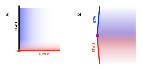
Figure 1: Two possible cobordism interpretations of intersecting ETW branes: a) The ETW₂ brane defines a cobordism to nothing for the configuration of the bulk theory ending at the ETW₁ brane boundary. b)The bulk theory ends on a cobordism to nothing boundary which switches from and ETW₁ brane to and ETW₂ brane.

The full expicit solutions we construct have a remarkably simple structure, realizing a superposition of the individual ETW branes, and are fully characterized by the individual critical exponents. In fact we compute the source terms and find they correspond to localized terms associated to the ETW brane tension and scalar couplings, with no additional source terms localized at their intersection.

Our approach should be regarded as local near the intersection, in the spirit of Angius:2022aeq , and similarly leads to a universal scaling properties. We explore them in the context of versions of the Distance Conjecture in theories with multiple scalars, including the Convex Hull formulation Calderon-Infante:2020dhm .

Although we do not expect our solutions to provide the most general intersecting ETW brane solutions, we show that they include a rich set of physically relevant systems, such as intersecting Witten’s bubbles of nothing Witten:1981gj (see Blanco-Pillado:2023aom ; Blanco-Pillado:2023hog ; Sugimoto:2023oul ; Delgado:2023uqk for recent related systems) in toroidal compactifications, or generalizations in compactifications in products of spheres, possibly dressed with fluxes (and hence including D-brane sources at the ETW brane). The setup also provides an arena for the actual exploration of the network of infinite distance loci in CY moduli spaces, which will be discussed in Angius:2024 .

For simplicity we mostly focus on configurations of two ETW branes intersecting orthogonally (see Blumenhagen:2000dc ; Dudas:2002dg ; Blumenhagen:2022mqw ; Blumenhagen:2023abk for other discussions of codimension-2 solutions), but also present generalizations for more than two ETW branes, and for general angles. We also compare our solutions with intersecting ETW branes associated to the same scalar, and show the latter actually are better regarded as singular limits of a single recombined ETW brane. This fits with the interpretation in Angius:2022mgh for a particular example with tachyon condensation in supercritical strings.

A cosmological application of our solutions would be the description of collisions of cosmological bubbles (see Kleban:2011pg for a review). It would be interesting to exploit our local models to extract universal signatures of these phenomena. We leave the exploration of phenomenological applications of our solutions to future work.

The paper is organized as follows. In section 2 we review the codimension-1 ETW brane solution, following Angius:2022aeq . In section 3 we construct the intersecting ETW brane solutions and discuss their properties. The ansatz and explicit solutions are constructed in section 3.1, section 3.2 discusses the associated ETW brane worldvolume source terms, and in section 3.3 we describe the scaling properties of the class of solutions. Section 4 contains explicit examples, including intersections of Witten’s bubbles of nothing in ${\bf{S}}^{1}\times{\bf{S}}^{1}$ compactifications (section 4.1), and in ${\bf{S}}^{p_{1}}\times{\bf{S}}^{p_{2}}$ compactifications (section 4.2), ETW branes with charged D-brane defects (section 4.3), and the intersection of a bubble of nothing with a general ETW brane (section 4.4). In section 5 we discuss the interplay with swampland constraints, including the cobordism conjecture (section 5.1), the distance conjecture (section 5.2), including the convex hull formulation in Calderon-Infante:2020dhm and the infinite distance pattern in Castellano:2023stg ; Castellano:2023jjt . Finally, we offer some concluding remarks in section 6. Appendix A discusses several generalizations and related systems, including intersections at general angles (section A.1), intersections of more than two ETW branes (section A.2), and intersecting ETW branes with a single scalar (section A.3)

2 Overview of codimension-1 ETW branes

In this section we overview the local description for codimension-1 ETW branes in Angius:2022aeq . Consider $d$-dimensional gravity coupled to a real scalar $\phi$ with general potential

$$S=\int d^{d}x\,\sqrt{-g}\,\left(\frac{1}{2}R-\frac{1}{2}\left(\partial\phi\right)^{2}-V(\phi)\right)\,,$$ (2.1)

Here and in the rest of this work we set $M_{Pl}=1$ units and consider $d>2$. The scalar may correspond to a combination of underlying moduli/scalar fields.

The codimension-1 ETW brane solution has the structure

$$ds^{2}_{d} = e^{-2\sigma(y)}ds_{d-1}^{2}+dy^{2}\,,$$

$$\phi = \phi(y)\,,$$ (2.2)

As pioneered in Buratti:2021fiv , the dynamical cobordism is characterized by the scalar $\phi$ going off to infinite distance in field space $\phi\to\infty$ at finite distance in spacetime $y\to 0$. Imposing the equations of motion, the local description near the ETW brane is

$$\phi(y) \simeq -\frac{2}{\delta}\log y$$

$$\sigma(y) \simeq -\frac{4}{(d-2)\delta^{2}}\,\log y\,+\frac{1}{2}\log c\,,$$ (2.3)

where the parameter $\delta$ describes the leading exponential behaviour of the potential

$$V(\varphi)=-ace^{\delta\varphi}$$ (2.4)

with $c$ a free parameter and $a$ is related to $\delta$ by

$$\delta=\sqrt{\frac{d-1}{d-2}(1-a)}$$ (2.5)

As explained in Angius:2022aeq the above solution leads to universal scaling relations among the spacetime distance to the singularity $\Delta$, the traverse scalar field space distance ${\cal D}$ and the spacetime curvature scalar, in terms of the parameter $\delta$:

$$\Delta\sim e^{-\frac{1}{2}\delta{\cal D}},\quad|R|\sim e^{\delta{\cal D}}.$$ (2.6)

A general warning, for these solutions and those in coming sections, is that at infinity in field space one expects the theory to have a lowered cutoff, which limits the validity of the effective field theory. Indeed, the appearance of corrections at the species scale has been discussed in small black holes in Calderon-Infante:2023uhz , and we may expect similar phenomena in ETW brane solutions. Still, effective field theory remains a useful tool to describe the systems, and even to quantify these corrections. Our solutions in this work should be understood in this spirit.

We now discuss a simple example of ETW brane, given by an analogue of the bubble of nothing of ${\bf{S}}^{1}$ compactifications Witten:1981gj , with the role of the expanding bubble replaced by a flat static wall of nothing (see Angius:2022aeq for the spherical bubble case).

We start with $(d+1)$-dimensional gravity with an action

$$S_{d+1}=\frac{1}{2}\int d^{d+1}x\sqrt{-g}R.$$ (2.7)

We consider compactifying on ${\bf{S}}^{1}$ parametrized by $\theta$, with the compactification ansatz

$$ds_{d+1}^{2}=e^{\alpha\rho}ds_{d}^{2}+e^{-\beta\rho}d\theta^{2}.$$ (2.8)

The parameters $\alpha$, $\beta$ are fixed by requiring the $d$-dimensional metric is in the Einstein frame, and by fixing the normalization of the radion kinetic term. We have

$$\beta=(d-2)\alpha\quad,\quad\alpha^{2}=\frac{4}{(d-1)(d-2)}\,.$$ (2.9)

The resulting $d$-dimensional action is

$$S=\frac{1}{2}\int d^{d}x\,\sqrt{-g}\,\big{[}R-(\partial\rho)^{2}\big{]}\,.$$ (2.10)

The theory is like (2.1) with the scalar $\phi=\rho$ and zero potential, since ${\bf{S}}^{1}$ has no curvature. It thus admits a solution of the kind (2.2), (2.3) with

$$\delta=2\sqrt{\frac{d-1}{d-2}}.$$ (2.11)

It is easy to uplift this solution and check that it corresponds to taking an ${\bf{S}}^{1}$ slicing of $(d+1)$ dimensional flat space

$$ds_{d+1}^{2}=ds_{d-1}^{2}+dr^{2}+r^{2}d\theta^{2},$$ (2.12)

with $ds_{d-1}^{2}$ describing a flat metric along the ETW brane worldvolume, and $r$ and $y$ related by

$$y=\left(\frac{d-2}{d-1}\right)r^{\frac{d-1}{d-2}}.$$ (2.13)

We refer to Angius:2022aeq for other examples, some of which will be arise as building blocks in our examples of intersecting ETW branes in section 4. We now turn to the general description of codimension-2 intersections of ETW branes.

3 Intersecting ETW branes

In this section we consider configurations describing the intersection of two ETW branes of the kind considered in the previous section. As we will see, they remarkably satisfy a simple superposition ansatz. This is reminiscent of the superposition of harmonic functions for supergravity solutions of (suitably smeared) intersecting BPS branes, with the differences that we do not require supersymmetry of the solutions, or even of the underlying theory, and that our solutions are fully localized and require no smearing.

We note that we focus on solutions describing the local behaviour near the intersection. The global structure in a general setup may differ in a model-dependent way. Hence, we focus on the universal behaviour of the configurations, much in the spirit of Angius:2022aeq for the codimension-1 case.

3.1 Codimension-2 ansatz and solutions

We consider the following $(n+2)$-dimensional action for gravity coupled to two real scalars with a general potential $V(\phi_{1},\phi_{2})$:

$$S=\int d^{n+2}x\sqrt{-g}\left\{\frac{1}{2}R-\frac{1}{2}\left(\partial\phi_{1}\right)^{2}-\frac{1}{2}\left(\partial\phi_{2}\right)^{2}-\frac{\alpha}{2}\partial_{\rho}\phi_{1}\partial^{\rho}\phi_{2}-V(\phi_{1},\phi_{2})\right\}.$$ (3.1)

Note that we have introduced a mixed kinetic term, which could be removed by diagonalization. However, maintaining it will allow for a simpler solution for the scalar profiles. As in the codimension-1 case in section 2, the scalars can be combinations of several moduli/scalar fields.

The above action is regarded as describing the theory around the infinite distance locus. An important observation in this respect is that we are using a locally flat metric around that point. Points at infinity are actually singular in general, but can admit such description if one restricts to specific directions in field space. An illustrative example is provided by considering two complex scalars $\Phi$ with Kähler potential

$$K=\log(\Phi_{1}+{\overline{\Phi}}_{1})+\log(\Phi_{1}+{\overline{\Phi}}_{2}).$$ (3.2)

Introducing the axion and saxion components $\Phi_{i}=\varphi_{i}+it_{i}$, the metric is given by two decoupled hyperbolic spaces

$$\frac{1}{t_{1}^{2}}\left(\,dt_{1}^{2}+d\varphi_{1}^{2}\,\right)+\frac{1}{t_{2}^{2}}\left(\,dt_{2}^{2}+d\varphi_{2}^{2}\,\right)=d\phi_{1}^{2}+d\phi_{2}^{2}+e^{-2\phi_{1}}d\varphi_{1}^{2}+e^{-2\phi_{2}}d\varphi_{2}^{2},$$ (3.3)

where we have introduced the canonically normalized saxion fields $\phi_{i}=\log t_{i}$. Clearly, the metric for the axions $\varphi_{i}$ is singular at the infinite distance locus for $\phi_{i}\to\infty$. On the other hand, restricting to solutions where the axions are inactive, the dynamics for the saxions is controlled by flat metric kinetic terms. The action (3.1) should be understood as describing such smooth slices around the infinite distance point .

In order to solve the equations of motion for the above action, we consider the ansatz for the metric:

$$ds^{2}_{n+2}=e^{2A(y_{1},y_{2})}ds^{2}_{n}+e^{2B(y_{1},y_{2})}dy_{1}^{2}+e^{2C(y_{1},y_{2})}dy_{2}^{2}\,,$$ (3.4)

and for the profiles of the two scalars:

$$\phi_{1}=\phi_{1}(y_{1})\quad,\quad\quad\quad\phi_{2}=\phi_{2}(y_{2}).$$ (3.5)

A linear independent set of combinations of the equations of motion is

$$\begin{split}(1)\quad&e^{-2C}n\left[n\left(A^{\prime}\right)^{2}+A^{\prime}\left(B^{\prime}-C^{\prime}\right)+A^{\prime\prime}\right]+e^{-2B}n\left[n\left(\dot{A}\right)^{2}+\dot{A}\left(\dot{C}-\dot{B}\right)+\ddot{A}\right]=-2V,\\ (2)\quad&e^{-2C}\left[-n\left(A^{\prime}\right)^{2}+(n-2)A^{\prime}\left(B^{\prime}-C^{\prime}\right)+(n-2)A^{\prime\prime}+2B^{\prime}\left(B^{\prime}-C^{\prime}\right)+2B^{\prime\prime}+\left(\phi_{2}^{\prime}\right)^{2}\right]+\\ +&e^{-2B}\left[-n\left(\dot{A}\right)^{2}+(n-2)\dot{A}\left(\dot{C}-\dot{B}\right)+(n-2)\ddot{A}+2\dot{C}\left(\dot{C}-\dot{B}\right)+2\ddot{C}+\left(\dot{\phi_{1}}\right)^{2}\right]=0,\\ (3)\quad&n\left[\dot{A}B^{\prime}-\dot{A}A^{\prime}+\dot{C}B^{\prime}-\dot{A}^{\prime}\right]=\frac{\alpha}{2}\dot{\phi_{1}}\phi_{2}^{\prime},\\ (4)\quad&e^{-2B}\left[\left(n\dot{A}-\dot{B}+\dot{C}\right)\dot{\phi_{1}}+\ddot{\phi_{1}}\right]+\frac{\alpha}{2}e^{-2C}\left[\left(nA^{\prime}+B^{\prime}-C^{\prime}\right)\phi_{2}^{\prime}+\phi_{2}^{\prime\prime}\right]-\frac{\partial V}{\partial\phi_{1}}=0,\\ (5)\quad&e^{-2C}\left[\left(nA^{\prime}+B^{\prime}-C^{\prime}\right)\phi_{2}^{\prime}+\phi_{2}^{\prime\prime}\right]+\frac{\alpha}{2}e^{-2B}\left[\left(n\dot{A}-\dot{B}+\dot{C}\right)\dot{\phi_{1}}+\ddot{\phi_{1}}\right]-\frac{\partial V}{\partial\phi_{2}}=0,\end{split}$$ (3.6)

where we have introduced the notation $\dot{f}\equiv\partial_{y_{1}}f$, $f^{\prime}\equiv\partial_{y_{2}}f$.
In particular, eq.$(1)$ is proportional to the sum of the $\{y_{1}y_{1}\}$ and $\{y_{2}y_{2}\}$ components of the Einstein equations. Eq.$(2)$ is the $\{ij\}$ component, using eq.$(1)$ to eliminate the potential. Eq.$(3)$ is the mixed $\{y_{1}y_{2}\}$component, and eqs.$(4)$ and $(5)$ are the equations of motion for the scalars.

We are interested in solutions describing intersecting ETW branes, with the requirement that each scalar $\phi_{i}$ runs off to infinite distance in field space as it approaches the origin in the coordinate $y_{i}$ it depends on; consequently both scalars diverge at the codimension-2 locus $y_{1}=y_{2}=0$. This is depicted in Figure 2.

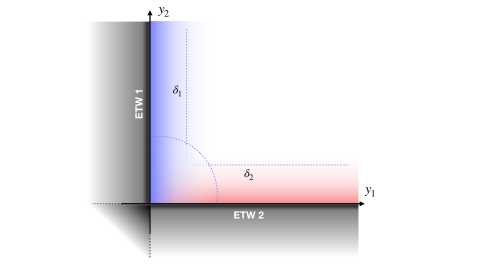
Figure 2: Intersection of two orthogonal ETW branes of type $\delta_{1}$ and $\delta_{2}$. Our solutions zoom into the region near the intersection, denoted with a dashed curve.

Let us emphasize again that the solution is intended to be a local description near the intersection point. Hence the center piece of Figure 2 is meant to describe a local patch near the intersection where this local description holds.

A simple proposal for the solution to describe two intersecting ETW branes is that for e.g. constant non-zero $y_{2}$, one recovers a codimension-1 ETW brane solution (and similarly for $y_{1}$). Hence, the metric should be of the form (2.2). This is achieved if we impose an additive structure in our warp factors

$$A(y_{1},y_{2})=-\sigma_{1}(y_{1})-\sigma_{2}(y_{2})\quad,\quad B(y_{1},y_{2})=-\sigma_{2}(y_{2})\quad,\quad C(y_{1},y_{2})=-\sigma_{1}(y_{1}).$$ (3.7)

Note that we have not included additive factors depending on $y_{1}$ on $B$, or on $y_{2}$ on $C$, since they can be reabsorbed by redefining those coordinates. In fact, the above parametrization makes the connection with (2.2) manifest. The metric (3.4) becomes

$$ds_{n+2}^{2}\,=\,e^{-2\sigma_{1}-2\sigma_{2}}ds_{n}^{2}\,+\,e^{-2\sigma_{2}}dy_{1}^{2}\,+\,e^{-2\sigma_{1}}dy_{2}^{2}\,,$$ (3.8)

so that for e.g. in a constant non-zero $y_{2}$ slice, the resulting $(n+1)$-dimensional metric is (up to a constant)

$$ds_{n+1}^{2}\,=\,e^{-2\sigma_{1}}ds_{n}^{2}\,+\,dy_{1}^{2}\,$$ (3.9)

with a running scalar $\phi_{1}(y_{1})$, and $\phi_{2}$ remains constant along the slice. This is precisely the structure of the local description of a codimension-1 ETW brane. Obviously, a similar pattern holds for constant $y_{1}$ slices. Motivated by this, we can propose logarithmic profiles for the functions $\sigma_{i}$, $\phi_{i}$:

$$\sigma_{1}=-a_{1}\log y_{1}+\frac{1}{2}\log c_{1},\quad\quad \sigma_{2}=-a_{2}\log y_{2}+\frac{1}{2}\log c_{2},$$ (3.10)

$$\phi_{1}=b_{1}\log y_{1},\quad\quad\quad\quad\ \quad\quad \phi_{2}=b_{2}\log y_{2},$$

where $c_{1}$ and $c_{2}$ correspond to (subleading) constant terms related to the two independent integration constants of the equations of motion.

Replacing these profiles in (3.6), we get the following constraints:

$$V = -\frac{1}{2}c_{1}na_{1}[\,(n+1)a_{1}-1\,]y_{1}^{-2}y_{2}^{-2a_{2}}-\frac{1}{2}c_{2}na_{2}[\,(n+1)a_{2}-1\,]y_{1}^{-2a_{1}}y_{2}^{-2}$$

$$\equiv -c_{1}v_{1}y_{1}^{-2}y_{2}^{-2a_{2}}-c_{2}v_{2}y_{1}^{-2a_{1}}y_{2}^{-2}$$

$$\alpha = 2\sqrt{a_{1}a_{2}}$$

$$b_{i}^{2} = na_{i}$$ (3.11)

Note the prefactors in the scalar potential, which are controlled by the constants $c_{i}$ in the logarithmic ansatz (3.10). In the first equation, assuming $a_{1},a_{2}\neq 1$, the potential splits in two pieces with different dependence on $y_{1},y_{2}$. We thus split

$$V=V_{1}+V_{2}\quad,\quad V_{1}\sim-c_{1}v_{1}\,y_{1}^{-2}y_{2}^{-2a_{2}}\quad,\quad V_{2}\sim c_{2}v_{2}\,y_{1}^{-2a_{1}}y_{2}^{-2}$$ (3.12)

Note that the asymptotic behaviour of $V$ fixes the values of $a_{1},a_{2}$ and then there is no freedom to change $\alpha$. Hence this class of solutions requires a tuning of the mixed kinetic term for the scalars. This may seem a strong restriction on the theory; however, starting from a theory with e.g. no mixed terms, one can always redefine the scalars such that the appropriate mixed term arises. Hence the above condition can be regarded as specifying in which basis of the scalar fields the solution takes the above simple form. Interestingly we will show that the above set of solutions includes large classes of interesting examples, as we describe in section 4.

Using the above, we get

$$a_{1}=\frac{1\pm\sqrt{1+8v_{1}\left(1+\frac{1}{n}\right)}}{2(n+1)}\quad,\quad a_{2}=\frac{1\pm\sqrt{1+8v_{2}\left(1+\frac{1}{n}\right)}}{2(n+1)}$$ (3.13)

In analogy with the codimension-1 ETW branes, we introduce the quantities $\delta_{1}$, $\delta_{2}$, such that the local ansatz reads

$$V = V_{1}+V_{2}=c_{1}v_{1}\,e^{\delta_{1}\phi_{1}}e^{a_{2}\delta_{2}\phi_{2}}+c_{2}v_{2}\,e^{a_{1}\delta_{1}\phi_{1}}e^{\delta_{2}\phi_{2}}$$

$$\phi_{1} = -\frac{2}{\delta_{1}}\log y_{1}\quad,\quad\phi_{2}=-\frac{2}{\delta_{2}}\log y_{2}$$

$$\sigma_{1} = -\frac{4}{n\delta_{1}^{2}}\log y_{1}\quad,\quad\sigma_{2}=-\frac{4}{n\delta_{2}^{2}}\log y_{2}$$ (3.14)

This is the codimension-2 local description of intersecting ETW branes, which generalizes the structure of the local description for codimension-1 ETW branes in Angius:2022aeq . The full solution is determined by the critical exponents $\delta_{i}$ associated with the two individual ETW branes. From the above equations, they are given by

$$\delta_{1}^{2}=\frac{8(n+1)}{n\pm\sqrt{n\left[n+8v_{1}(n+1)\right]}}\quad,\quad\delta_{2}^{2}=\frac{8(n+1)}{n\pm\sqrt{n\left[n+8v_{2}(n+1)\right]}}.$$ (3.15)

Let us mention that our solution is even more general than what the derivation above suggests. Indeed, if one starts from (3.4) and requires a general additive structure with independent functions (i.e. beyond (3.7)) with general logarithmic profiles, the equations of motion end up leading to the above solution. Hence, (3.7) can be regarded as a derived structure, once the logarithmic profiles are imposed.

We incidentally note that the ansatz (3.8) is conformally flat, generalizing the situation encountered in the codimension-1 case in section 2. This is easily shown by changing to new coordinates $x^{1}$, $x^{2}$ such that

$$dy_{1}=e^{-\sigma_{1}}dx_{1}\quad,\quad dy_{2}=e^{-\sigma_{2}}dx_{2}$$ (3.16)

so that (3.8) becomes

$$ds_{n+2}^{2}\,=\,e^{-2\sigma_{1}-2\sigma_{2}}\,[\,ds_{n}^{2}\,+\,dx_{1}^{2}\,+\,dx_{2}^{2}\,]\,.$$ (3.17)

where $\sigma_{i}$ are obviously regarded as functions of $x^{i}$. Conformally flat codimension-2 solutions have been discussed in setups with a single scalar e.g. in Dudas:2002dg . It would be interesting to explore possible relations between the two setups.

For our purposes, the expression (3.17) will allow to generalize our solutions to ETW branes intersecting at general angles in appendix A.1. In coming sections we restrict to orthogonal intersections (3.8) for simplicity, the generalization being trivial.

3.2 The sources

In this section we discuss the source terms that correspond to our above intersecting ETW brane solutions, and check that they are just a superposition of source terms at $y_{1}=0$ and at $y_{2}=0$ closely related to the source terms of codimension-1 ETW branes. In particular, there is no further source term localized purely at the intersection $y_{1}=y_{2}=0$. For simplicity of the discussion, we focus on the case of zero scalar potential; the general case can be worked out similarly.

We start with recovering the source term for the codimension-1 ETW brane solutions following Blumenhagen:2023abk (see also Blumenhagen:2000dc ; Blumenhagen:2022mqw ; Sugimoto:2023oul ; Delgado:2023uqk ). We start with the $d$-dimensional action with a source term describing the tension and coupling to the scalar of the ETW brane:

$$\centering S=\int d^{d}x\sqrt{-g}\,\bigg{[}\,\frac{1}{2}R-\frac{1}{2}\left(\partial\phi\right)^{2}\,\bigg{]}-\lambda\int d^{d-1}x\sqrt{-\tilde{g}}\,e^{\tilde{\alpha}\phi}\delta(y),\@add@centering$$ (3.18)

where now $\tilde{g}$ denotes the pullback of the $d$-dimensional metric $g$ to the worldvolume of the codimension-1 defect. Using the ansatz (2.2), the two equations of motion coming from the variation with respect to the metric become:

$$\begin{split}\{i,j\}:\ \ &\frac{1}{2}\phi^{\prime 2}+\frac{(d-1)(d-2)}{2}\sigma^{\prime 2}-(d-2)\sigma^{\prime\prime}+\lambda e^{\tilde{\alpha}\phi}\delta(y)=0,\\ \{y,y\}:\ \ &\phi^{\prime 2}-(d-1)(d-2)\sigma^{\prime 2}=0,\end{split}$$ (3.19)

where the prime denotes derivation with respect to $y$. The variation of the action with respect to the field $\phi$ gives:

$$\phi^{\prime\prime}-(d-1)\phi^{\prime}\sigma^{\prime}=\tilde{\alpha}\lambda e^{\tilde{\alpha}\phi}\delta(y).$$ (3.20)

Making the ansatz $\phi=-\sqrt{\frac{d-2}{d-1}}f(y)$ and $\sigma=-\frac{1}{d-1}f(y)$ automatically satisfies the $\{y,y\}$ equation of motion, and the remaining two equations read:

$$\begin{split}&\frac{d-2}{d-1}\big{(}f^{\prime 2}+f^{\prime\prime}\big{)}=-\lambda e^{\tilde{\alpha}\phi}\delta(y),\\ &\sqrt{\frac{d-2}{d-1}}\big{(}f^{\prime 2}+f^{\prime\prime}\big{)}=-\tilde{\alpha}\lambda e^{\tilde{\alpha}\phi}\delta(y).\end{split}$$ (3.21)

By direct comparison one can read off the value of $\tilde{\alpha}$

$$\tilde{\alpha}=\sqrt{\frac{d-1}{d-2}}.$$ (3.22)

Setting now $f(y)=\log(h(y))$ (with $h(y)\geq 0$) this becomes

$$\frac{h^{\prime\prime}}{h}=-\lambda\frac{d-1}{d-2}e^{-\log h}\delta(y)\,\quad\Rightarrow\quad\,h^{\prime\prime}=-\lambda\,\frac{d-1}{d-2}\,\delta(y)\,.$$ (3.23)

Now we can integrate this over $[0,x_{0})$ and take the limit $x_{0}\to 0$. The left hand side is just the discontinuity of $h^{\prime}$. Using the solution to the equations of motion, for $y<0$ we take $h=1$, so that $f(y)=0$ and all fields vanish beyond the ETW brane, while for $y>0$, $h=y-y_{0}$, with $y_{0}$ an integration constant (with $y_{0}<0$ to have $h(y)\geq 0$ near $y=0$), which we will eventually take to $y_{0}\to 0^{-}$ to match our solution.

Then after the integration/limit we have:

$$1=-\frac{d-1}{d-2}\lambda\quad\Rightarrow\quad\lambda=-\frac{d-2}{d-1}.$$ (3.24)

The negative tension of this ETW brane was already explicitly noticed in Blumenhagen:2023abk (see also Delgado:2023uqk ), for the physical choice of signs we have implicitly assumed in our solution.

We now turn to the intersecting ETW-brane solution, and show that codimension-1 sources of the kind studied above suffice to support the solution. We thus use a $d$-dimensional action (and set $d=n+2$) including sources of the following form:

$$\centering\begin{split}S&=\int d^{n+2}x\sqrt{-g}\left\{\frac{1}{2}R-\frac{1}{2}\left(\partial\phi_{1}\right)^{2}-\frac{1}{2}\left(\partial\phi_{2}\right)^{2}-\frac{\alpha}{2}\partial_{\rho}\phi_{1}\partial^{\rho}\phi_{2}\right\}\\ &-\lambda_{1}\int d^{n+1}x\sqrt{-g_{1}}e^{\alpha_{11}\phi_{1}+\alpha_{12}\phi_{2}}\delta(y_{1})-\lambda_{2}\int d^{n+1}x\sqrt{-g_{2}}e^{\alpha_{22}\phi_{2}+\alpha_{21}\phi_{1}}\delta(y_{2})\,.\end{split}\@add@centering$$ (3.25)

where $g_{i}$, $i=1,2$ is the pullback of the metric on the worldvolume of the $(n+1)$-dimensional ETW branes. Note that we have not included a term $\delta(y_{1})\delta(y_{2})$, as it is not necessary (in fact, it is forced to be absent) in our solution.

The equations of motion arising from the variation of the above action are very similar to those of (3.6), when appropriately replacing the potential with the source terms. Using the ansatz (3.4) for the metric and the additive structure (3.7) for the warp factors, the equations of motion coming from the variations of (3.25) with respect to the metric components are:

$$\begin{split}\{i,j\}:\ \ \frac{1}{2}\Big{[}&e^{-2\sigma_{1}}\Big{(}\dot{\phi}_{1}^{2}+n(n+1)\dot{\sigma}_{1}^{2}-2n\ddot{\sigma}_{1}\Big{)}+e^{-2\sigma_{2}}\Big{(}\phi_{2}^{\prime 2}+n(n+1)\sigma_{2}^{\prime 2}-2n\sigma_{2}^{\prime\prime}\Big{)}\Big{]}\\ +&\lambda_{1}e^{\alpha_{11}\phi_{1}+\alpha_{12}\phi_{2}}e^{-2\sigma_{1}-\sigma_{2}}\delta(y_{1})+\lambda_{2}e^{\alpha_{22}\phi_{2}+\alpha_{21}\phi_{1}}e^{-\sigma_{1}-2\sigma_{2}}\delta(y_{2})=0,\\ \{y_{1},y_{1}\}:\ \ &\frac{1}{2}\Big{[}-\dot{\phi}_{1}^{2}+n(n+1)\dot{\sigma}_{1}^{2}+e^{2\sigma_{1}-2\sigma_{2}}\big{(}\phi_{2}^{\prime 2}+n(n+1)\sigma_{2}^{\prime 2}-2n\sigma_{2}^{\prime\prime}\big{)}\Big{]}\\ &\ \ \ \ \ +\lambda_{2}e^{\alpha_{22}\phi_{2}+\alpha_{21}\phi_{1}}e^{-2\sigma_{2}+\sigma_{1}}\delta(y_{2})=0,\\ \{y_{2},y_{2}\}:\ \ &\frac{1}{2}\Big{[}-\phi_{2}^{\prime 2}+n(n+1)\sigma_{2}^{\prime 2}+e^{-2\sigma_{1}+2\sigma_{2}}\big{(}\dot{\phi}_{1}^{2}+n(n+1)\dot{\sigma}_{1}^{2}-2n\ddot{\sigma}_{1}\big{)}\Big{]}\\ &\ \ \ \ \ +\lambda_{1}e^{\alpha_{11}\phi_{1}+\alpha_{12}\phi_{2}}e^{-2\sigma_{1}+\sigma_{2}}\delta(y_{1})=0,\\ \{y_{1},y_{2}\}:\ \ &-n\dot{\sigma}_{1}\sigma_{2}^{\prime}+\frac{1}{2}\alpha\dot{\phi}_{1}\phi_{2}^{\prime}=0.\end{split}$$ (3.26)

Additionally, one has two equations of motion coming from the variations with respect to the fields $\phi_{i}$:

$$\begin{split}\phi_{1}:\ \ &e^{-\sigma_{1}+\sigma_{2}}\big{(}-(n+1)\dot{\phi}_{1}\dot{\sigma}_{1}+\ddot{\phi}_{1}\big{)}+\frac{\alpha}{2}e^{\sigma_{1}-\sigma_{2}}\big{(}-(n+1)\phi_{2}^{\prime}\sigma_{2}^{\prime}+\phi_{2}^{\prime\prime}\big{)}\\ -&\alpha_{11}\lambda_{1}e^{\alpha_{11}\phi_{1}+\alpha_{12}\phi_{2}}e^{-\sigma_{1}}\delta(y_{1})-\alpha_{21}\lambda_{2}e^{\alpha_{22}\phi_{2}+\alpha_{21}\phi_{1}}e^{-\sigma_{2}}\delta(y_{2})=0,\\ \phi_{2}:\ \ &\frac{\alpha}{2}e^{-\sigma_{1}+\sigma_{2}}\big{(}-(n+1)\dot{\phi}_{1}\dot{\sigma}_{1}+\ddot{\phi}_{1}\big{)}+e^{\sigma_{1}-\sigma_{2}}\big{(}-(n+1)\phi_{2}^{\prime}\sigma_{2}^{\prime}+\phi_{2}^{\prime\prime}\big{)}\\ -&\alpha_{12}\lambda_{1}e^{\alpha_{11}\phi_{1}+\alpha_{12}\phi_{2}}e^{-\sigma_{1}}\delta(y_{1})-\alpha_{22}\lambda_{2}e^{\alpha_{22}\phi_{2}+\alpha_{21}\phi_{1}}e^{-\sigma_{2}}\delta(y_{2})=0.\end{split}$$ (3.27)

In analogy with the codimension-1 case, let us make the change $\phi_{i}=-\sqrt{\frac{n}{n+1}}f_{i}(y_{i})$, $\sigma_{i}=-\frac{1}{n+1}f_{i}$ to simplify the equations,

in particular the $\{y_{1},y_{2}\}$ equation in (3.26) is satisfied identically. Each of the remaining equations splits into two contributions depending on each the two coordinates, provided that $\alpha_{21}\phi_{1}=\sigma_{1}$ and $\alpha_{12}\phi_{2}=\sigma_{2}$, hence

$$\alpha_{12}=\alpha_{21}=\frac{1}{\sqrt{n(n+1)}}.$$ (3.28)

For the scalar equations (3.27) to be compatible one needs

$$\alpha=\frac{2}{n+1}.$$ (3.29)

which corresponds to the appropriate value for the case of vanishing potential. The set of equations decouples into two sets basically identical to the codimension-1 equations (3.21) for the $f_{i}$, namely

$$\begin{split}&\frac{n}{n+1}\left(f_{i}^{\prime 2}+f_{i}^{\prime\prime}\right)=-\lambda_{i}e^{\alpha_{ii}\phi_{i}}\delta(y_{i}),\\ &\sqrt{\frac{n}{n+1}}\left(f_{i}^{\prime 2}+f_{i}^{\prime\prime}\right)=-\alpha_{ii}\lambda_{i}e^{\alpha_{ii}\phi_{i}}\delta(y_{i}),\end{split}$$ (3.30)

with no sum over $i$, and where prime denotes derivative with respect to their argument, now also for $f_{1}(y_{1})$. The equations can be analyzed as in the codimension-1 case, so their compatibility requires

$$\alpha_{11}=\alpha_{22}=\sqrt{\frac{n+1}{n}}=\sqrt{\frac{d-1}{d-2}}$$ (3.31)

and the computation of the discontinuities imply

$$\lambda_{1}=\lambda_{2}=-\frac{n-1}{n}=-\frac{d-2}{d-1},$$ (3.32)

just like in the codimension-1 case, c.f. (3.24).

Hence the sources are a simple superposition of two terms along $y_{i}=0$, with tensions $\lambda_{i}$ and couplings $\alpha_{ii}$ to the scalar $\phi_{i}$ given by those of the corresponding codimension-1 ETW brane solution. The extra coupling $\alpha_{12}$ of the ETW brane along $y_{1}=0$ to $\phi_{2}$, and $\alpha_{21}$ of the ETW along $y_{2}=0$ to $\phi_{1}$ imply an interesting variation of the effective tension of the ETW branes as one moves further away from the intersection. Morally, it accounts for the extra factor involved in expressing the codimension-2 solution as a codimension-1 solution, mentioned just above (3.9).

Let us finally explain the solution leaves no room for a codimension-2 $\delta(y_{1})\delta(y_{2})$ source term. Such term would lead to discontinuities in mixed derivatives of the fields, which are absent in the equations of motion (3.26), (3.27). This is already built in from the use of the additive structure (3.7). It would be interesting to explore more general solutions involving this extra sources, but this lies beyond the scope of this work.

3.3 Scaling relations

In this section we discuss the analogue of the scaling relations (2.6), in particular the relation between the spacetime distance to the singularity along some path and the traversed scalar field space distance. Clearly, the relation will be path-dependent, albeit in a simple way.

Consider a general path $y_{i}(t)$ in spacetime, parametrized by $t$, with $y^{i}\to 0$ as $t\to 0$. For instance, we can choose

$$y_{1}=t^{\gamma_{1}}\quad,\quad y_{2}=t^{\gamma_{2}}$$ (3.33)

in terms of two positive real numbers $\gamma_{i}\geq 0$. Clearly, a change $t\to t^{\lambda}$ is just a reparametrization of the same path, so $\gamma_{i}$ are defined up to an overall rescaling, so only its ratio is meaningful. The tangent vector is

$$\partial_{t}y_{i}=\gamma_{i}\,t^{\gamma_{i}-1}.$$ (3.34)

The spacetime distance to the origin along this path is

$$\Delta = \int[\,e^{-2\sigma_{2}}(\partial_{t}y_{1})^{2}+e^{-2\sigma_{1}}(\partial_{t}y_{2})^{2}\,]^{\frac{1}{2}}\,dt\,=\,\,\int[\,\gamma_{1}^{2}t^{2r_{1}}+\gamma_{2}^{2}t^{2r_{2}}\,]^{\frac{1}{2}}\,dt$$ (3.35)

with

$$r_{1}=\frac{4\gamma_{2}}{n\delta_{2}^{2}}+\gamma_{1}-1\quad,\quad r_{2}=\frac{4\gamma_{1}}{n\delta_{1}^{2}}+\gamma_{2}-1$$ (3.36)

We can consider two regimes, depending on which contribution dominates in the $t\to 0$ limit. The two regions are separated by the line $r_{1}=r_{2}$, equivalently

$$\frac{\gamma_{1}}{\gamma_{2}}\,=\,\frac{\frac{4}{n\delta_{2}^{2}}-1}{\frac{4}{n\delta_{1}^{2}}-1}.$$ (3.37)

The two regimes correspond to the path being closer to each of the two ETW branes. Assuming $r_{1}\neq r_{2}$, the spacetime distance in the two regions is given by

$$\Delta=\int\gamma_{i}\,t^{r_{i}}\,dt=\frac{\gamma_{i}}{r_{i}+1}t^{r_{i}+1}.$$ (3.38)

We incidentally note that the $r_{i}$ have a natural interpretation by writing the tangent vector (3.34) in the tangent space frame $\tau^{a}=e_{i}^{a}\partial_{t}y_{i}$ with $e_{i}^{a}$ defined by $G_{ij}=e_{i}^{a}e_{j}^{b}\delta_{ab}$

$$\vec{\tau}=(e^{-\sigma_{2}}\partial_{t}y_{1},e^{-\sigma_{1}}\partial_{t}y_{2})=(\gamma_{1}t^{r_{1}},\gamma_{2}t^{r_{2}}).$$ (3.39)

Products of vectors in the tangent space are with the flat metric $\delta_{ab}$, so this reproduces the distance element (3.35). The tangent vector $\vec{\tau}$ will play an interesting role in the discussion of the Distance Conjecture in section 5.2.

The profiles for the scalars allow to translate the path $y_{i}(t)$ in spacetime into a path in field space $\phi_{i}(y(t))$. Let us now compute the field theory distance traversed along the path from a point located at some small non-zero value $t$ to the origin $t=0$. From the action (3.1), the line element in field space is given by

$$d{\cal D}^{2} = d\phi_{1}^{2}+d\phi_{2}^{2}+\alpha d\phi_{1}d\phi_{2}=4\left(\frac{\gamma_{1}^{2}}{\delta_{1}^{2}}+\frac{\gamma_{2}^{2}}{\delta_{2}^{2}}+\frac{\alpha\gamma_{1}\gamma_{2}}{\delta_{1}\delta_{2}}\right)\frac{dt^{2}}{t^{2}}.$$ (3.40)

This can be recast in terms of the spacetime distance, for each of the two regions in (3.38), as

$${\cal D}=-2\left(\frac{\gamma_{1}^{2}}{\delta_{1}^{2}}+\frac{\gamma_{2}^{2}}{\delta_{2}^{2}}+\frac{\alpha\gamma_{1}\gamma_{2}}{\delta_{1}\delta_{2}}\right)^{\frac{1}{2}}\log t\sim-\frac{2}{|r_{i}+1|}\left(\frac{\gamma_{1}^{2}}{\delta_{1}^{2}}+\frac{\gamma_{2}^{2}}{\delta_{2}^{2}}+\frac{\alpha\gamma_{1}\gamma_{2}}{\delta_{1}\delta_{2}}\right)^{\frac{1}{2}}\log\Delta.\quad\quad$$ (3.41)

The explicit dependence on the parametrization i.e. on the $\gamma_{i}$, is simply due to the fact that the choice of initial point for the computation of the distance in terms of a value $t$ does depend on the parametrization (3.33).

We thus obtain a scaling relation near the intersection, of the kind (2.6), namely

$$\Delta\sim e^{-\frac{1}{2}\delta_{\rm int}\,{\cal D}}\,,$$ (3.42)

with a path-dependent coefficient, which in each of the two regions reads

$$\delta_{\rm int}=\left(\frac{\gamma_{1}^{2}}{\delta_{1}^{2}}+\frac{\gamma_{2}^{2}}{\delta_{2}^{2}}+\frac{\alpha\gamma_{1}\gamma_{2}}{\delta_{1}\delta_{2}}\right)^{-\frac{1}{2}}(r_{i}+1).$$ (3.43)

This interpolates between the values of the critical exponents of the two individual ETW branes, which are attained for paths orthogonal to the individual ETW branes:

$$\begin{split}\gamma_{1}=1\;,&\;\gamma_{2}=0\quad\quad\Rightarrow\quad\delta_{\rm int}\to\delta_{1}\\ \gamma_{1}=0\;,&\;\gamma_{2}=1\quad\quad\Rightarrow\quad\delta_{\rm int}\to\delta_{2}\\ \end{split}$$ (3.44)

In order to visualize the interpolation, let us parametrize $\gamma_{1}=\sqrt{\gamma}$ and $\gamma_{2}=1/\sqrt{\gamma}$ such that we have the ratio $\gamma_{1}/\gamma_{2}=\gamma$. The value of $\gamma$ separating the two regimes is (3.37). In terms of this parametrization, we have

$$\delta_{int}=\begin{cases}&\left(\frac{\gamma}{\delta_{1}^{2}}+\frac{1}{\gamma\delta_{2}^{2}}+\frac{\alpha}{\delta_{1}\delta_{2}}\right)^{-1/2}\left(\sqrt{\gamma}+\frac{4}{n\delta_{2}^{2}\sqrt{\gamma}}\right)\quad\quad\quad\text{for }\gamma>\gamma^{\ast}\\ &\left(\frac{\gamma}{\delta_{1}^{2}}+\frac{1}{\gamma\delta_{2}^{2}}+\frac{\alpha}{\delta_{1}\delta_{2}}\right)^{-1/2}\left(\frac{1}{\sqrt{\gamma}}+\frac{4\sqrt{\gamma}}{n\delta_{1}^{2}}\right)\quad\quad\quad\quad\text{for }\gamma<\gamma^{\ast}.\\ \end{cases}$$ (3.45)

Note that we recover the limits $\delta_{1}$, $\delta_{2}$ for $\gamma\mapsto\infty,0$, respectively.

Consider for instance the case $\delta_{1}=\delta_{2}\equiv\delta$. The two regimes are separated by $\gamma^{\ast}=1$ and the scaling parameter simplifies:

$$\delta_{int}=\begin{cases}&\left[1+\gamma(\gamma+\alpha)\right]^{-1/2}\left(\frac{4+n\gamma\delta^{2}}{n\delta}\right)\quad\quad\text{for }\gamma>1\\ &\left[1+\gamma(\gamma+\alpha)\right]^{-1/2}\left(\frac{4\gamma+n\delta^{2}}{n\delta}\right)\quad\quad\text{for }\gamma<1.\\ \end{cases}$$ (3.46)

For $\delta_{1}\neq\delta_{2}$ the separation between the two regimes lies at $\gamma^{\ast}\neq 1$. In Figures 3 we display $\delta_{\rm int}$ as a function of $\log\gamma$, for some illustrative examples with equal (figure a) or different (figure b) values of $\delta_{1},\delta_{2}$.

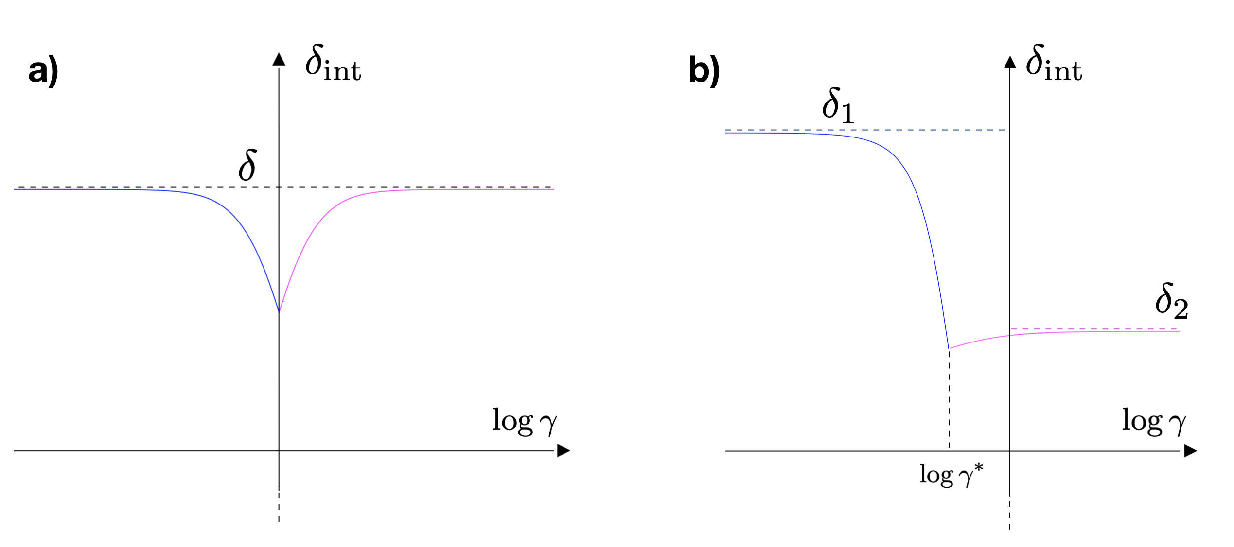
Figure 3: Plot of $\delta_{int}$ as a function of the path for two illustrative examples with $\delta_{1}=\delta_{2}\equiv\delta$

(figure a) and $\delta_{1}\neq\delta_{2}$ (figure b).

The scaling properties between the spacetime and field theory distance will play an important role in the discussion of swampland conjectures in section 5. In the following section we turn to show several explicit examples of systems described by the solution we have discussed.

4 Explicit examples

In this section we consider explicit examples of intersecting ETW brane solutions. Many are simply obtained from simple configurations, like flat space, by considering reduction along some isometry orbits, which potentially diverge at large distances from the intersection. The solutions we describe should be regarded as local descriptions near the intersection of more involved solutions where such orbits have finite size at infinity. We will mention explicit realizations for several of our examples.

4.1 ${\bf S}^{1}\times{\bf S}^{1}$ compactifications

A simple example of a codimension-1 ETW brane is the wall of nothing in ${\bf{S}}^{1}$ compactifications (analogue of the bubble of nothing in Witten:1981gj ) described in section 2. From the higher-dimensional perspective, the local description corresponds to taking flat space, splitting of an ${\bf{R}}^{2}$, and slicing it along the angular ${\bf{S}}^{1}$, regarding it as a compactification circle, with radius varying along the radial coordinate, c.f. (2.12).

In the same spirit, we can consider the intersection of two wall of nothing ETW branes, which provides a local model for two intersecting bubbles of nothing for different ${\bf{S}}^{1}$’s. The idea is simply to consider the flat $(n+4)$-dimensional space, written as

$$ds_{n+4}^{2}=ds_{n}^{2}+dr_{1}^{2}+dr_{2}^{2}+r_{1}^{2}d\theta_{1}^{2}+r_{2}^{2}d\theta_{2}^{2}$$ (4.1)

where $ds_{n}^{2}$ is just flat $n$-dimensional space.

The above will soon be rewritten in the Einstein frame of the $(n+2)$-dimensional theory obtained upon reduction on the ${\bf{S}}^{1}\times{\bf{S}}^{1}$ parametrized by $\theta_{i}$; but the intuition is already clear. We have an $(n+2)$-dimensional theory with two scalars, the ${\bf{S}}^{1}$ sizes, depending of two coordinates $r_{i}$. Each scalar shrinks to zero size at the codimension-1 locus $r_{1}=0$ or $r_{2}=0$, respectively, and both shrink simultaneously at the codimension-2 locus $r_{1}=r_{2}=0$.

We now turn to carrying this out explicitly. We start with $(n+4)$-dimensional gravity with action

$$S_{n+4}=\frac{1}{2}\int d^{n+4}x\sqrt{-g_{n+4}}\,R_{n+4}$$ (4.2)

and compactify on ${\bf{S}}^{1}\times{\bf{S}}^{1}$, parametrized by coordinates $\theta_{1}$, $\theta_{2}$. We consider the following ansatz for the $(n+2)$-dimensional theory:

$$ds^{2}_{n+4}=e^{\alpha_{1}\rho_{2}+\alpha_{2}\rho_{2}}ds^{2}_{n+2}+e^{-\beta_{1}\rho_{1}}d\theta_{1}^{2}+e^{-\beta_{2}\rho_{2}}d\theta_{2}^{2},$$ (4.3)

where the breathing modes $\rho_{i}$ are functions of the non-compact $n+2$ dimensions. The parameters are fixed by the $(n+2)$-dimensional Einstein frame condition, and normalization of the scalar kinetic terms, giving

$$n\alpha_{i}=\beta_{i}\quad,\quad\beta_{i}^{2}=\frac{4n}{n+1}.$$ (4.4)

Upon compactification, the $(n+2)$-dimensional action for these fields is

$$S_{n+2} \propto \frac{1}{2}\int d^{n+2}x\sqrt{-g_{n+2}}\big{[}\,R_{n+2}-|d\rho_{1}|^{2}-|d\rho_{2}|^{2}-\alpha\partial_{\mu}\rho_{1}\partial^{\mu}\rho_{2}\,\big{]}\,,$$ (4.5)

with

$$\alpha=\frac{2}{n+1}.$$ (4.6)

This corresponds to an action of the kind (3.1), with the two scalars corresponding to the ${\bf{S}}^{1}$ sizes, namely $\phi_{i}\equiv\rho_{i}$. The scalar potential is zero because the ${\bf{S}}^{1}$’s have no curvature.

The flat space slicing (4.1) corresponds to an intersecting ETW brane solution of the kind in section 3 with

$$ds^{2}_{n+2} = r_{1}^{\frac{2}{n}}r_{2}^{\frac{2}{n}}\left(\eta_{\mu\nu}dx^{\mu}dx^{\nu}+dr_{1}^{2}+dr^{2}_{2}\right),$$

$$\phi_{1} = -\sqrt{\frac{n+1}{n}}\log r_{1}\quad,\quad\phi_{2}=-\sqrt{\frac{n+1}{n}}\log r_{2}.$$ (4.7)

With a change of variables

$$y_{i}=\,\frac{n}{n+1}\,r_{i}^{\frac{n+1}{n}}\,,$$ (4.8)

we can go from the above conformally flat solution to one of the form (3.4) with

$$ds_{n+2}^{2} = y_{1}^{\frac{2}{n+1}}y_{2}^{\frac{2}{n+1}}\,ds_{n}^{2}\,+\,y_{2}^{\frac{2}{n+1}}dy_{1}^{2}\,+\,y_{1}^{\frac{2}{n+1}}dy_{2}^{2},$$

$$\phi_{i} = -\sqrt{\frac{n}{n+1}}\log y_{i}.$$ (4.9)

This corresponds to the critical exponents

$$\delta_{i}=2\sqrt{\frac{n+1}{n}}.$$ (4.10)

4.2 ${\bf{S}}^{p_{1}}\times{\bf{S}}^{p_{2}}$ compactifications

We now consider a generalization of the above example, by starting with an $D$-dimensional space, with $D=n+2+p_{1}+p_{2}$, and compactifying on ${\bf{S}}^{p_{1}}\times{\bf{S}}^{p_{2}}$. The intersecting ETW brane solution, in which the ${\bf{S}}^{p_{1}}$ and ${\bf{S}}^{p_{2}}$ shrink to zero size at two interescting codimension-1 loci, is locally given by slicing $D$-dimensional flat space as

$$ds^{2}_{D}=\eta_{\mu\nu}dx^{\mu}dx^{\nu}+dr_{1}^{2}+dr_{2}^{2}+r_{1}^{2}d\Omega_{p_{1}}^{2}+r_{2}^{2}d\Omega_{p_{2}}^{2},$$ (4.11)

where $x^{\mu}$ are coordinates along the Poincaré invariant directions along the intersection and $d\Omega_{p_{1}}^{2}$ and $d\Omega_{p_{2}}^{2}$ are the line elements in ${\bf{S}}^{p_{1}}$ and ${\bf{S}}^{p_{2}}$, respectively.

Let us quickly describe this construction. We start with $D$-dimensional gravity with action

$$S_{D}=\frac{1}{2}\int d^{D}x\sqrt{-g_{D}}R_{D}.$$ (4.12)

The compactification ansatz is

$$ds^{2}_{D}=e^{\alpha_{1}\rho_{2}+\alpha_{2}\rho_{2}}ds^{2}_{n+2}+e^{-\beta_{1}\rho_{1}}d\Omega^{2}_{p_{1}}+e^{-\beta_{2}\rho_{2}}d\Omega^{2}_{p_{2}},$$ (4.13)

with the requirement to land on the $(n+2)$-dimensional Einstein frame leading to

$$n\alpha_{i}=p_{i}\beta_{i}.$$ (4.14)

Also, we normalize the kinetic terms of the two radions $\rho_{i}$ via the following relations:

$$\beta_{i}^{2}=\frac{4n}{p_{i}(n+p_{i})}$$ (4.15)

The $(n+2)$-dimensional Einstein frame action for gravity and the two radions is

$$S_{n+2} \propto \frac{1}{2}\int d^{n+2}x\sqrt{-g_{n+2}}\Big{[}\,R_{n+2}-|d\rho_{1}|^{2}-|d\rho_{2}|^{2}-\alpha\partial_{\mu}\rho_{1}\partial^{\mu}\rho_{2}$$ (4.16)

$$+\frac{p_{1}(p_{1}-1)}{R_{p_{1}}^{2}}e^{(\alpha_{1}+\beta_{1})\rho_{1}+\alpha_{2}\rho_{2}}+\frac{p_{2}(p_{2}-1)}{R^{2}_{p_{2}}}e^{\alpha_{1}\rho_{1}+(\alpha_{2}+\beta_{2})\rho_{2}}\Big{]}\,,$$

with

$$\alpha=\frac{2{\sqrt{p_{1}p_{2}}}}{\sqrt{(n+p_{1})(n+p_{2})}}.$$ (4.17)

The action (4.16) has precisely the structure (3.1) with the two radions corresponding to the two scalars i.e. $\phi_{i}\equiv\rho_{i}$, which have an exponential potential due to the curvature of the internal spheres.

The flat space slicing (4.11) provides a solution to this theory with the structure (3.8), (3.10) with

$$ds_{n+2}^{2} = y_{1}^{\frac{2p_{1}}{p_{1}+n}}y_{2}^{\frac{2p_{2}}{p_{2}+n}}\,,ds_{n}^{2}\,+\,y_{2}^{\frac{2p_{2}}{p_{2}+n}}dy_{1}^{2}\,+\,y_{1}^{\frac{2p_{1}}{p_{1}+n}}dy_{2}^{2},$$

$$\phi_{i} = -\sqrt{\frac{np_{i}}{n+p_{i}}}\log y_{i}.$$ (4.18)

This corresponds to the critical exponents

$$\delta_{i}=2\sqrt{\frac{n+p_{i}}{np_{i}}}.$$ (4.19)

The ${\bf{S}}^{1}\times{\bf{S}}^{1}$ example in section 4.1 is clearly recovered for $p_{1}=p_{2}=1$.

One particular example realizing this local behaviour (albeit with AdS₄ rather than 4d Poincaré invariance along the ETW brane) is the gravity dual of 4d ${\cal{N}}=4$ $SU(N)$ SYM with a boundary coupled to a 3d ${\cal{N}}=4$ BCFT Gaiotto:2008sa ; Gaiotto:2008ak . It is given by the supergravity solution of D3-branes ending on NS5- and D5-branes), see DHoker:2007zhm ; DHoker:2007hhe ; Aharony:2011yc ; Assel:2011xz ; Assel:2012cj ; Bachas:2017rch ; Bachas:2018zmb ; Raamsdonk:2020tin ; VanRaamsdonk:2021duo ; Huertas:2023syg , which as emphasized in Raamsdonk:2020tin ; VanRaamsdonk:2021duo ; Huertas:2023syg corresponds to an ETW brane in AdS${}_{5}\times{\bf{S}}^{5}$. It is described as an AdS₄ times $({\bf{S}}^{2})^{2}$ fibered over a Riemann surface given by the first quadrant $(y_{1},y_{2})$ with $y_{i}\geq 0$. The two ${\bf{S}}^{2}$’s shrink to zero size at $y_{1}=0$ and $y_{2}=0$ respectively, while both shrink simultaneously at $y_{1}=y_{2}=0$ (so, together with the polar angle in the $(y_{1},y_{2})$-plane, there is a shrinking ${\bf{S}}^{5}$). Hence, this setup reproduces locally the structure of our solution, while globally provides an explicit example in which the ${\bf{S}}^{2}$’s have constant radius at infinity (being part of the constant radius ${\bf{S}}^{5}$ in the asymptotic AdS${}_{5}\times{\bf{S}}^{5}$).

4.3 Adding D-brane defects

The above examples correspond to variants of bubbles of nothing, in which the ETW brane is realized geometrically, by shrinking (parts of) the compact space. In general, one expects ETW branes to be dressed with topological defects necessary to remove non-trivial cobordism charges of the compactification. A prototypical example is compactifications with field strength fluxes, which require the presence of charged branes at the ETW brane to remove the flux. In this section we consider a simple example describing the local behaviour of an ETW brane for a compactification on ${\bf{S}}^{8-p}$ with $N$ units of RR flux (hence the ETW brane is dressed with $N$ D$p$-branes) intersecting an ETW brane of a fluxless ${\bf{S}}^{q}$ (i.e. a bubble of nothing).

Actually, the solution is described by simply taking the solution for a stack of $N$ D$p$-branes in flat space. For simplicity we focus on $p<7$, for which the metric and dilaton read

$$\begin{split}&ds^{2}_{10}=Z(r_{1})^{\frac{p-7}{8}}(\eta_{\mu\nu}dx^{\mu}dx^{\nu}\,+\,dr_{2}^{2}+r_{2}^{2}d\Omega_{q}^{2})+Z(r_{1})^{\frac{p+1}{8}}\left(dr_{1}^{2}+r_{1}^{2}d\Omega^{2}_{8-p}\right),\\ &\Phi=\frac{(3-p)}{4\sqrt{2}}\log Z(r_{1}),\\ &Z(r_{1})=1+\left(\frac{\rho}{r_{1}}\right)^{7-p}\quad,\quad\rho^{7-p}=g_{s}N\alpha^{\prime(7-p)/2}(4\pi)^{(5-p)/2}\Gamma\left(\frac{7-p}{2}\right)\,.\end{split}$$ (4.20)

Here $x^{\mu}$ parametrize $p-q$ of the D$p$-brane worlvolume directions, and $r_{2}$ is the radial coordinate in the remaining ${\bf{R}}^{p+1}$ part of the worldvolume, and $d\Omega_{q}^{2}$ is the line element in the angular ${\bf{S}}^{q}$. Namely, we slice the D$p$-brane solution along the transverse ${\bf{S}}^{8-p}$ and a worldvolume ${\bf{S}}^{q}$, and regard it as a solution of an ${\bf{S}}^{8-p}\times{\bf{S}}^{q}$ compactification.

We thus start with the 10d action for gravity coupled to the dilaton and the RR $(p+1)$-form

$$S_{10}\sim\frac{1}{2}\int d^{10}x\sqrt{-g_{10}}\left\{R_{10}-|d\Phi|^{2}-\frac{1}{2(8-p)!}e^{a\Phi}|F_{8-p}|^{2}\right\}$$ (4.21)

with

$$a=\frac{p-3}{2}.$$ (4.22)

We use the compactification ansatz

$$\begin{split}&ds^{2}_{10}=e^{\alpha_{1}\rho_{1}+\alpha_{2}\rho_{2}}ds^{2}_{n+2}+e^{-\beta_{1}\rho_{1}}d\Omega^{2}_{8-p}+e^{\gamma_{1}\rho_{1}-\gamma_{2}\rho_{2}}d\Omega^{2}_{q}\\ &F_{8-p}={N}dVol\left(S^{8-p}\right).\end{split}$$ (4.23)

We now impose the Einstein frame condition, and fix the normalization of the scalars $\rho_{i}$

$$\begin{split}&\beta_{1}=\frac{n\alpha_{1}+q\gamma_{1}}{8-p}=\frac{1}{8+n-p}\left[(p-n)\gamma_{1}\pm 2\frac{\sqrt{n\left[8+n-p+2(p-n)\gamma_{1}^{2}\right]}}{\sqrt{8-p}}\right]\\ &\gamma_{2}=\frac{n}{q}\alpha_{2}=\pm 2\sqrt{\frac{n}{q(n+q)}}\\ \end{split}$$ (4.24)

The resulting $(n+2)$-dimensional action (with $n=p-q$) is:

$$\begin{split}&S_{n+2}=\frac{1}{2}\,{\cal C}\!\int d^{n+2}x\sqrt{-g_{n+2}}\left\{R_{n+2}-|d\Phi|^{2}-|d\rho_{1}|^{2}-|d\rho_{2}|^{2}+\frac{\gamma_{2}q\left[\beta_{1}(p-8)+\gamma_{1}p\right]}{2n}\partial_{\mu}\rho_{1}\partial^{\mu}\rho_{2}+\right.\\ &\left.+(8-p)(7-p)e^{(\alpha_{1}+\beta_{1})\rho_{1}+\alpha_{2}\rho_{2}}+q(q-1)e^{(\alpha_{1}-\gamma_{1})\rho_{1}+(\alpha_{2}+\gamma_{2})\rho_{2}}-\frac{N^{2}}{2(8-p)!}e^{a\Phi}e^{\left[\alpha_{1}+(8-p)\beta_{1}\right]\rho_{1}+\alpha_{2}\rho_{2}}\right\},\\ \end{split}$$ (4.25)

with the coefficient

$${\cal C}=\left(\frac{2\pi^{(8-p)/2}}{\Gamma\left(\frac{(8-p)}{2}\right)}\right)\left(\frac{2\pi^{q/2}}{\Gamma\left(\frac{q}{2}\right)}\right).$$ (4.26)

We can now write this in the form (3.1) using the redefinitions

$$\phi_{1} = \int\left[|d\Phi|^{2}+|d\rho_{1}|^{2}\right]^{1/2}$$

$$\phi_{2} = \rho_{2}$$ (4.27)

and the following relation between the $10$ dimensional dilaton and the radion:

$$\Phi=\sqrt{2}\frac{(p-7)}{(p-3)}\rho_{1},$$ (4.28)

from which we have:

$$\phi_{1}=\left[1-2\frac{\gamma_{1}}{\beta_{1}}\right]^{1/2}\rho_{1}.$$ (4.29)

The action becomes:

$$\begin{split}&S_{n+2}=\frac{\mathcal{C}}{2}\int d^{n+2}x\sqrt{-g_{n+2}}\left\{R_{n+2}-|d\phi_{1}|^{2}-|d\phi_{2}|^{2}-\alpha\partial_{\rho}\phi_{1}\partial^{\rho}\phi_{2}+\right.\\ &\left.+\frac{(8-p)(7-p)}{R^{2}_{8-p}}e^{\frac{1}{n}\left(1-2\frac{\gamma_{1}}{\beta_{1}}\right)^{-1/2}\left[(8+n-p)\beta_{1}+(n-p)\gamma_{1}\right]\phi_{1}}e^{2\sqrt{\frac{q}{n(n+q)}}\phi_{2}}\right.+\\ &+\frac{q(q-1)}{R^{2}_{q}}e^{\frac{1}{n}\left(1-2\frac{\gamma_{1}}{\beta_{1}}\right)^{-1/2}\left[(8-p)\beta_{1}-p\gamma_{1}\right]\phi_{1}}e^{2\sqrt{\frac{n+q}{nq}}\phi_{2}}+\\ &\left.-\frac{N^{2}}{2(8-p)!}e^{\left\{\frac{(p-3)}{2}\left(1-\frac{1}{2}\frac{\beta_{1}}{\gamma_{1}}\right)^{-1/2}-\frac{1}{n}\left(1-2\frac{\gamma_{1}}{\beta_{1}}\right)^{-1/2}\left[(n+1)(p-8)\beta_{1}+q\gamma_{1}\right]\right\}\phi_{1}}e^{2\sqrt{\frac{q}{n(n+q)}}\phi_{2}}\right\}\\ \end{split}$$ (4.30)

with

$$\alpha=\frac{\gamma_{2}q\left[\beta_{1}(8-p)-\gamma_{1}p\right]}{2n}\left(1-2\frac{\gamma_{1}}{\beta_{1}}\right)^{-1/2}.$$ (4.31)

The D$p$-brane solution descends to a solution of the kind (3.4) with the redefinitions

$$\begin{split}&y_{1}=\left(\frac{2n}{9+n(p-5)-p}\right)r_{1}^{\frac{9+n(p-5)-p}{2n}},\\ &y_{2}=\left(\frac{n}{q+n}\right)r_{2}^{\frac{q}{n}+1}.\\ \end{split}$$ (4.32)

The solution corresponds to

$$ds_{n+2}^{2}=e^{-2\sigma_{1}-2\sigma_{2}}ds^{2}_{n}+e^{-2\sigma_{2}}dy_{1}^{2}+e^{-2\sigma_{1}}dy_{2}^{2},$$ (4.33)

$$\phi_{1}=-\sqrt{\frac{n(9-p)}{9+n(p-5)-p}}\log y_{1},$$ (4.34)

$$\phi_{2}=-\sqrt{\frac{qn}{q+n}}\log y_{2},$$ (4.35)

$$\sigma_{1}=-\frac{(9-p)}{9+n(p-5)-p}\log y_{1},$$ (4.36)

$$\sigma_{2}=-\frac{q}{q+n}\log y_{2}.$$ (4.37)

Hence the resulting critical exponents are

$$\delta_{1}=2\sqrt{\frac{9+n(p-5)-p}{n(9-p)}}\quad,\quad\delta_{2}=2\sqrt{\frac{q+n}{qn}}.$$ (4.38)

4.4 One general ETW brane

In this section we present a generalization of the previous sections, and consider the intersection of a bubble of nothing ETW brane, corresponding to a shrinking ${\bf{S}}^{p}$, with a completely general ETW brane characterized by a critical exponent $\delta$. The solution is actually very simple. We start with a theory in $d=n+p+2$ dimensions and action

$$S_{d}=\int d^{d}x\sqrt{-g}\left[\frac{1}{2}R-\frac{1}{2}\left(\partial\varphi\right)^{2}-V(\varphi)\right]$$ (4.39)

We consider a general codimension-1 local ETW brane solution as in (2.2), (2.3), sliced along an angular ${\bf{S}}^{p}$ on its worldvolume dimensions, namely

$$\begin{split}&ds^{2}_{d}=e^{-2\sigma(y)}\,[\,ds_{n}^{2}+dr^{2}+r^{2}d\Omega_{p}^{2}\,]\,+dy^{2}\\ &\varphi(y)\simeq-\frac{2}{\delta}\log y\quad,\quad\sigma(y)\simeq-\frac{4}{(d-2)\delta^{2}}\log y,\\ \end{split}$$ (4.40)

The potential in the regime near the ETW brane is of the exponential form (2.4):

$$V(\varphi)=-ace^{\delta\varphi}.$$ (4.41)

Taking the coordinate $r$ to parametrize a coordinate along with the ${\bf{S}}^{p}$ varies, this realizes the intersection of ETW branes of interest.

In order to describe it from the perspective of the $(n+2)$-dimensional action after reduction along the ${\bf{S}}^{p}$, we take the compactification ansatz

$$ds^{2}_{d}=e^{\alpha\rho}ds^{2}_{n+2}+e^{-\beta\rho}d\Omega^{2}_{p},$$ (4.42)

The coefficients $\alpha$, $\beta$ are fixed by the Einstein frame condition in $(n+2)$-dimensional action and the normalization of the scalar $\rho$. We require

$$n\alpha=p\beta\quad,\quad\beta^{2}=\frac{4n}{p(p+n)}.$$ (4.43)

The resulting $(n+2)$-dimensional action is

$$\begin{split}S_{n+2}&=\frac{1}{2}\int d^{n+2}x\sqrt{-g_{n+2}}\Big{\{}R_{n+2}-\left(\partial\varphi\right)^{2}-\left(\partial\rho\right)^{2}+\frac{p(p-1)}{R^{2}_{p}}e^{2\sqrt{\frac{n+p}{np}}\rho}+\\ &\left.-2V(\varphi)e^{2\sqrt{\frac{p}{n(n+p)}}\rho}\right\},\\ \end{split}$$ (4.44)

where $\varphi$ is the scalar associated to the generic ETW brane in $d-$dimensions and $\rho$ is the breathing mode of the ${\bf{S}}^{p}$ compactification. In order to get an action in the form (3.1), we redefine the fields via:

$$\varphi=\delta\sqrt{\frac{n(n+p)}{4p+n(n+p)\delta^{2}}}\,\phi_{1}\quad,\quad\rho=\phi_{2}+2\sqrt{\frac{p}{4p+n(n+p)\delta^{2}}}\,\phi_{1}\,,$$ (4.45)

and the (4.44) becomes:

$$\begin{split}&S_{n+2}=\frac{1}{2}\int d^{n+2}x\sqrt{-g_{n+2}}\Big{\{}R_{n+2}-\left(\partial\phi_{1}\right)^{2}-\left(\partial\phi_{2}\right)^{2}-\alpha\partial_{\rho}\phi_{1}\partial^{\rho}\phi_{2}+\\ &\left.+\frac{p(p-1)}{R^{2}_{p}}e^{2\sqrt{\frac{n+p}{np}}\left(\phi_{2}-2\sqrt{\frac{p}{4p+n(n+p)\delta^{2}}}\phi_{1}\right)}+2ace^{2\sqrt{\frac{p}{n(n+p)}}\phi_{2}+\sqrt{\frac{4p+n(n+p)\delta^{2}}{n(n+p)}}\phi_{1}}\right\},\\ \end{split}$$ (4.46)

with

$$\alpha=2\sqrt{\frac{p}{4p+n(n+p)\delta^{2}}}.$$ (4.47)

It is easy to check that the configuration (4.40) is a local intersecting ETW brane solution (3.14). Performing the change of variables

$$y_{1}=\left(\frac{n(n+p)\delta^{2}}{4p+n(n+p)\delta^{2}}\right)y^{\frac{4p}{n(n+p)\delta^{2}}+1}\quad,\quad y_{2}=\left(\frac{n}{p+n}\right)r^{\frac{p}{n}+1}$$ (4.48)

we obtain

$$ds_{n+2}^{2} = e^{-2\sigma_{1}-2\sigma_{2}}ds^{2}_{n}+e^{-2\sigma_{2}}dy_{1}^{2}+e^{-2\sigma_{1}}dy_{2}^{2}$$

$$\sigma_{1} = -\frac{4(n+p)}{\delta^{2}n(n+p)+4p}\log y_{1}\quad,\quad\sigma_{2}=-\frac{p}{n+p}\log y_{2}$$

$$\phi_{1} = -2\sqrt{\frac{n(n+p)}{4p+n(n+p)\delta^{2}}}\log y_{1}\quad,\quad\phi_{2}=-\sqrt{\frac{np}{n+p}}\log y_{2}$$ (4.49)

This corresponds to the critical exponents

$$\delta_{1}=\sqrt{\delta^{2}+\frac{4p}{n(n+p)}}\quad,\quad\delta_{2}=2\sqrt{\frac{n+p}{np}}.$$ (4.50)

Note that $\delta_{2}$ nicely agrees with the value obtained in section 4.2 c.f. (4.19). We can also recover examples of previous sections for different choices of $\delta$. For instance, for $\delta^{2}=4\frac{n+p+q}{q(n+p)}$ we recover the case of ${\bf{S}}^{p}\times{\bf{S}}^{q}$ compactification studied in section 4.2. Also, for $\delta^{2}=\frac{4(q-3)^{2}}{q(9-q)}$, with $q<7$, we recover the case of a D$q$-brane solution reduced along the transverse ${\bf{S}}^{8-q}$ times an ${\bf{S}}^{p}$ along the brane worldvolume, as studied in section 4.3 (with reversed labels $p$, $q$).

We hope that these examples suffice to illustrate that our class of solutions includes many physically relevant cases of ETW branes.

5 Swampland applications

In this section we discuss the interplay of our solutions with various swampland constraints. We mainly focus on the cobordism conjecture and the distance conjecture, but mention others along the way.

5.1 Cobordism conjecture

Since ETW branes are motivated by the Cobordism Conjecture, there are several interesting interpretations of our intersecting ETW brane solutions from this perspective.

5.1.1 The end of the world for end of the world branes

Dynamical cobordisms arise in the exploration of the Cobordism Conjecture McNamara:2019rup beyond its merely topological avatar. They provide explicit effective field theory descriptions of cobordisms to nothing, including the possibly necessary defects to remove any non-trivial cobordism classes or other charges in the configuration.

From the perspective of the effective theory, the microscopic structure of the cobordism defect remains mostly shrouded in the mist of the UV completion, but there may be features of the ETW brane worldvolume dynamics amenable to the effective theory approach. One way to probe them is to let the ETW brane interact with other defects of the theory. In the familiar context of string theory branes, the worldvolume gauge field content in a brane can be read from the objects able to end on it Strominger:1995ac , and some such BIon configurations are accessible in supergravity Gomberoff:1999ps . In the context of cobordism defects, for instance Dierigl:2023jdp obtained the type IIB R7-brane worldvolume theory by the characterization of branes allowed to end on its worldvolume. Namely, cobordism defects must be able to explain not just the end of bulk spacetime, but also the disappearance of the possible defects present in the bulk theory.

Intersecting ETW brane configurations can be regarded as a radical case of this last idea: Cobordism defects must be able to explain not just the end of bulk spacetime, but also of bulk configurations bounded by other pre-existing cobordism defects. From the effective theory perspective, when the bulk theory is bounded by a first ETW brane (ETW₁), the resulting configuration must admit being bounded by a second ETW brane (ETW₂), with the bulk ending on the ETW₂ brane and its boundary ETW₁ brane ending on its intersection with the ETW₂ brane, see Figure 1a. Obviously there is the converse picture, in which the ETW₁ brane provides a boundary of the configuration given by the bulk theory ending on the ETW₂ image. Hence our intersecting ETW brane solutions explain the end of the world for end of the world branes.

5.1.2 Interpolating Domain Walls between ETW branes

There is another related but complementary interpretation of intersecting brane configurations from the Cobordism Conjecture perspective, focusing on its implication that in theories of quantum gravity any two configurations can be connected by some domain wall. Hence we may consider two configurations given by the bulk theory bounded by the ETW₁ and the same bulk theory bounded by a different ETW₂ brane. We can now consider the interpolating configuration across which the bulk theory is unchanged but the ETW₁-brane turns into the ETW₂ brane. This can be regarded as a configuration of two intersecting ETW branes in the limit where their angle is close to $\pi$, with the intersection playing the role of interpolating domain wall between the ETW brane boundaries, see Figure 1b.

ETW branes at general angle $\theta$ are explicitly constructed in appendix A.1. The limit $\theta\to\pi$ is singular in that description, but only because the original coordinate system becomes degenerate. It would be interesting to extract the resulting limit configuration, or build its solution from scratch, but we refrain from doing so in the hope that the conceptual picture is clear enough.

The above links with the cobordism conjecture relate to the structure of spacetime and its boundaries (and boundaries of their boundaries). The realization of these configurations via dynamical cobordisms with scalars blowing up at the ETW branes furthermore leads to an in interesting map between spacetime physics and field space, to which we turn next.

5.2 Distance Conjecture

Our solutions are spacetime-dependent configurations probing infinite distance limits in field space at finite spacetime distance, and therefore have a direct interplay with the Distance Conjecture Ooguri:2006in . We explore various such connections in this section.

5.2.1 General Distance Conjecture

The Distance Conjecture Ooguri:2006in states that effective field theories break down along geodesic paths extending to infinite distance limits in moduli space due to the appearance of an infinite tower of states at a scale $m$ falling exponentially with the field theory distance

$$m\sim e^{-\lambda{\cal D}}$$ (5.1)

with some ${\cal O}(1)$ coefficient $\lambda$ (with $\lambda\geq\frac{1}{\sqrt{d-2}}$ according to the sharpened distance conjecture Etheredge:2022opl ).

In spacetime-dependent configurations probing infinite field space distances at finite spacetime distance, such as ETW branes Angius:2022aeq ; Blumenhagen:2022mqw ; Blumenhagen:2023abk , there are interesting relations between the field space distance and the spacetime distance, c.f. (2.6). This allows to provide a spacetime version of the Distance Conjecture which expresses the falloff of the cutoff scale along some path in spacetime.

In our intersecting ETW brane setup, we have found similar scaling relations between the field space distance and the spacetime distance (3.42), controlled by the path-dependent coefficient $\delta_{\rm int}$. Combining this expression with (5.1), we obtain

$$m\sim\Delta^{\frac{2\lambda}{\delta_{\rm int}}}$$ (5.2)

In spacetime-dependent solutions, i.e. beyond the adiabatic approximation, the interpretation of $m$ is not necessarily the appearance of an infinite tower Buratti:2018xjt ; it instead indicates the scale at which new UV physics kicks in. This played an important role in the context of small black holes, where it fixes the size of the smallest possible black hole in the effective theory Hamada:2021bbz ; Calderon-Infante:2023uhz . It would be interesting to explore similar mechanisms for ETW branes.

5.2.2 The Convex Hull Distance Conjecture

In theories with several scalar fields, there are different infinite distance limits, which probe the existence of different UV towers. Hence, the cutoff along general infinite distance path in field space can be sensitive to multiple individual towers. A general recipe to obtain the exponential falloff along such a general path is provided by the Convex Hull Distance Conjecture Calderon-Infante:2020dhm (see also Etheredge:2023odp ), as follows.

Consider all the towers of the theory corresponding to all possible infinite distance limits, and denote by $m(\phi^{i})$ the moduli-dependent mass scale of each of these towers. Let us introduce the scalar charge to mass ratios

$$\zeta_{i}\equiv\partial_{i}\log m.$$ (5.3)

Consider a trajectory $\phi^{i}(t)$ going to some infinite distance limit, and define the (normalized) tangent vector

$$\tau^{i}\equiv\frac{\phi^{\prime}{}^{i}}{||\phi^{\prime}||}\quad,\quad{\rm with}\;\phi^{\prime}{}^{i}=\frac{d\phi^{i}}{dt}$$ (5.4)

Along this trajectory the tower scale falls off as in (5.1) with

$$\lambda=-\zeta_{i}\,\tau^{i}=-\,\frac{\zeta_{i}\phi^{\prime}{}^{i}}{||\phi^{\prime}||}.$$ (5.5)

Notice that there is a dependence on the moduli space metric in the normalization of the tangent vector.

Introducing the tangent frame $e_{i}^{a}$ in field space $G_{ij}=\delta_{ab}e_{i}^{a}e_{j}^{b}$, and its inverse $e_{a}^{i}$, this can be recast in terms of vector scalar products

$$\lambda=-\zeta^{a}\tau_{a}\quad,\quad{\rm with}\;\zeta^{a}=e_{a}^{i}\zeta_{i}\;,\;\tau_{a}=e_{a}^{i}\tau_{i}.$$ (5.6)

Combining all towers, the falloff rate is controlled by the convex hull defined by the scalar charge to mass ratios for all towers in the theory Calderon-Infante:2020dhm .

We have shown that theories with several scalars admit intersecting ETW brane solutions, and that different spacetime paths approaching the intersection define different field space paths traversing infinite distance. Formally, one can regard the scalar profiles $\phi^{i}(y^{\mu})$ in our solution as defining an embedding of two spacetime dimensions into the scalar field space. This allows to define pullbacks of moduli space quantities onto the spacetime dimensions, and formulate a spacetime avatar of the Convex Hull Distance Conjecture.

Indeed, the pullback onto spacetime of the scalar charge to mass ratio is

$$\zeta_{\mu}=\partial_{\mu}\log m(\phi^{i}(x^{\mu}))=\partial_{\mu}\phi^{i}\,\zeta_{i}$$ (5.7)

Also, for a path in spacetime $x^{\mu}(\lambda)$, with (unnormalized) tangent vector

$$v^{\mu}=x^{\prime}{}^{\mu}(\lambda)\quad,\quad{\rm with}\;x^{\prime}{}^{\mu}=\frac{dx^{\mu}}{d\lambda}\,,$$ (5.8)

we get a path $\phi^{i}(x^{\mu}(\lambda))$ in field space, with (unnormalized) tangent vector

$$\frac{d}{d\lambda}\phi^{i}(x^{\mu}(\lambda))=\partial_{\mu}\phi^{i}\,x^{\prime}{}^{\mu}=\partial_{\mu}\phi^{i}\,v^{\mu}$$ (5.9)

We then have the spacetime version of the numerator of (5.5)

$$\zeta_{i}\,\phi^{\prime}{}^{i}\,=\,\zeta_{i}\partial_{\mu}\phi^{i}\,v^{\mu}=\zeta_{\mu}v^{\mu}$$ (5.10)

The Convex Hull criterion requires using normalized tangent vectors in field space. Using the scalar field metric $G_{ij}$, we have

$$||\phi^{\prime}||=(G_{ij}\phi^{\prime}{}^{i}\phi^{\prime}{}^{j})^{\frac{1}{2}}=(G_{ij}\partial_{\mu}\phi^{i}\partial_{\nu}\phi^{j}x^{\prime}{}^{\mu}x^{\prime}{}^{\nu})^{\frac{1}{2}}=(h_{\mu\nu}v^{\mu}v^{\nu})^{\frac{1}{2}}\,,$$ (5.11)

namely, the norm of $v^{\mu}$ but computed with the induced metric

$$h_{\mu\nu}=G_{ij}\partial_{\mu}\phi^{i}\partial_{\nu}\phi^{j}$$ (5.12)

Hence one can formulate the Distance Conjecture as a statement in spacetime in terms of the metric $h_{\mu\nu}$. Note that this is actually different from the spacetime metric $g_{\mu\nu}$. In particular, the field space metric contains mixed terms, whereas the actual spacetime metric is diagonal. It would be interesting to discuss dynamical properties in spacetime of this induced metric from the field space.

5.2.3 The infinite distance pattern

The above ideas can be easily extended to other swampland criteria. For instance, in Castellano:2023stg ; Castellano:2023jjt , an interesting pattern was proposed to hold at infinite distance limits (see also Rudelius:2023spc for proposals in the interior) between the tower scale $m(\phi^{i})$ and the species scale (the effective cutoff scale of quantum gravity Dvali:2007hz ; Dvali:2008ec ; Dvali:2009ks ; Dvali:2010vm ; Dvali:2012uq ) $\Lambda_{s}(\phi^{i})$, which in general is moduli-dependent. Specifically, they are claimed to satisfy

$$G^{ij}\,\partial_{i}\log m\,\partial_{j}\log\Lambda_{s}=\frac{1}{d-2}$$ (5.13)

In the context of our solutions, there is a spacetime version of this condition using the (inverse) induced metric

$$h^{\mu\nu}\,\partial_{\mu}\log m(\phi^{i}(y^{\mu}))\,\partial_{\nu}\log\Lambda_{s}(\phi^{i}(y^{\mu}))=\frac{1}{d-2}$$ (5.14)

Note that the species scale and its relation to the distance conjecture has already been studied from the perspective of the link between spacetime and field space structures for codimension-1 ETW brane solutions in Calderon-Infante:2023ler . We expect that similarly exciting ideas may arise in the codimension-2 case of intersecting ETW branes. We leave these explorations as well as links to other swampland conjectures for future work.

6 Conclusions

The exploration of infinite distance limits has led to the construction of diverse defects, such as ETW branes, small black holes or 4d EFT strings, defined by the fact that scalars reach infinite field theory distance at their cores. It is natural to ask about the interplay of such objects, and their use to explore the network of infinite field theory distance limits, i.e. their different components and their intersections.

In this paper we have initiated this exploration by constructing explicit solutions describing intersecting ETW branes in theories with multiple scalars. The configurations behave as the superposition of two codimension-1 ETW branes, and display interesting path-dependent scaling properties along trajectories approaching the codimension-2 intersection. We have explored the interplay of these solutions with swampland conjectures, and in particular with the convex hull description of the Distance Conjecture in theories with several scalars. Finally, we have explicitly shown that many interesting systems correspond to solutions within our class, including intersections of bubbles of nothing and several generalizations thereof.

Some of the interesting questions opened up by our work are:

$\bullet$ Our solutions can be regarded as a mere superposition of ETW branes, in the sense that their source terms are localized on the individual codimension-1 ETW branes. It would be interesting to describe more general intersections supported also by codimension-2 source terms. In this respect, it would be interesting to connect with the codimension-2 objects in Blumenhagen:2022mqw ; Blumenhagen:2023abk .

$\bullet$ There are localized D-brane solutions in the literature (see Ortin:2015hya for review and references), which upon suitable reductions along transverse space may be rephrased as intersections of codimension-1 ETW branes. However, the reduction involves directions along which there are no isometries and it is likely it leads to solutions not describable within our ansatz. It would be interesting to study these examples as a tool to generate more general solutions, in particular including examples with non-trivial degrees of freedom at the intersection of ETW branes.

$\bullet$ In our solutions the scalars diverging at the ETW branes had a non-trivial mixed kinetic term. It would be interesting to describe intersecting configurations for decoupled scalar fields, in particular to better connect with CY moduli spaces near infinite distance limits Grimm:2018ohb ; Grimm:2018cpv ; Corvilain:2018lgw . This will be addressed in Angius:2024 .

$\bullet$ We have focused on ETW branes and their interplay via intersections. More generally, it would be interesting to understand the interplay of other defects defined by scalars running off to infinity in field space. For instance, the crossing of two EFT strings may lead to the creation of new strings, unveiling non-abelian structures at infinity in moduli space, in the spirit of Berasaluce-Gonzalez:2012abm .

We hope to come back to these and other interesting questions in future work.

Appendix A Some generalizations

In this appendix we consider several generalizations and variants of the solutions discussed in the main text.

A.1 Intersection at angles

In the main text we have restricted the intersection of ETW branes to be orthogonal in the conformally flat coordinates (3.17). It is a natural generalization to consider a general off-diagonal term

$$ds_{n+2}^{2} = e^{-2\sigma_{1}-2\sigma_{2}}\,[\,ds_{n}^{2}\,+\,dx_{1}^{2}\,+\,dx_{2}^{2}\,+\,f\,dx_{1}dx_{2}\,]$$ (A.1)

$$= e^{-2\sigma_{1}-2\sigma_{2}}\,ds_{n}^{2}\,+\,e^{-2\sigma_{2}}\,dy_{1}^{2}\,+\,e^{-2\sigma_{1}}\,dy_{2}^{2}\,+\,f\,e^{-\sigma_{1}-\sigma_{2}}\,dy_{1}dy_{2}\,,$$

where $\sigma_{i}$ are regarded as functions of $x_{i}$ in the top line and of $y_{i}$ in the bottom one. We will look for solutions in which each scalar still runs along one coordinate $\phi_{1}(y_{1})$, $\phi_{2}(y_{2})$. In fact, we try and solve the equations of motion by using logarithmic profiles for $\sigma_{i}$ and $\phi_{i}$ as in (3.10), which we repeat for convenience

$$\sigma_{1}=-a_{1}\log y_{1}+\frac{1}{2}\log c_{1},\quad\quad\sigma_{2}=-a_{2}\log y_{2}+\frac{1}{2}\log c_{2},$$

$$\phi_{1}=b_{1}\log y_{1},\quad\quad\quad\quad\ \quad\quad\phi_{2}=b_{2}\log y_{2},$$ (A.2)

The equations of motion are satisfied if the coefficients satisfy:

$$b_{i}^{2}=na_{i}^{2}\quad,\quad\alpha=2\sqrt{a_{1}a_{2}}$$ (A.3)

and the potential behaves as

$$V=V_{1}+V_{2}+\mathcal{O}\left(y_{1}^{-1-a_{1}}y_{2}^{-1-a_{2}}\right)$$

$$V_{1}=c_{1}v_{1}y_{1}^{-2}y_{2}^{-2a_{2}}=\frac{2c_{1}na_{1}}{\left(f^{2}c_{1}c_{2}-4\right)}\left[(na_{1}+a_{1}-1)\right]y_{1}^{-2}y_{2}^{-2a_{2}}$$ (A.4)

$$V_{2}=c_{2}v_{2}y_{1}^{-2a_{1}}y_{2}^{-2a}=\frac{2c_{2}na_{2}}{\left(f^{2}c_{1}c_{2}-4\right)}\left[(na_{2}+a_{2}-1)\right]y_{1}^{-2a_{1}}y_{2}^{-2}$$ (A.5)

$$\mathcal{O}\left(y_{1}^{-1-a_{1}}y_{2}^{-1-a_{2}}\right)=-c_{1}c_{2}\frac{2n^{2}fa_{1}a_{2}}{\left(f^{2}c_{1}c_{2}-4\right)}y_{1}^{-1-a_{1}}y_{2}^{-1-a_{2}}$$ (A.6)

Note that the equations of motions provide us more than two terms for the potential. Assuming that $a_{1}<1$ and $a_{2}<2$, the last term is subleading respect to the previous ones which contain the information to specify the kind of intersecting ETW branes.

Moreover the coefficients are given by a generalization of (3.13), namely

$$a_{i}=\frac{n\pm\sqrt{n+2(n+1)v_{i}\left(f^{2}c_{1}c_{2}-4\right)}}{2n(n+1)}$$ (A.7)

Finally, the critical exponents are given by

$$\delta_{i}^{2}=\frac{4}{a_{1}n}=\frac{8(n+1)}{n\pm\sqrt{n+2(n+1)v_{i}(f^{2}c_{1}c_{2}-4)}}$$ (A.8)

Hence, even though (A.3) has the same structure as (3.11), there is a non-trivial dependence on $f$ in the potential and the coefficients of the logarithms. This implies that, given the potential of the theory, one can read off the values of $a_{i}$ and $v_{i}$ from its leading exponential behaviour, and determine the value (or values) of $f$ that provides a solution, which in general corresponds to non-orthogonal intersections.

Note that when $f^{2}c_{1}c_{2}-4=0$ the values above become singular. This corresponds to the limit where the angle between the two ETW branes is $0$ or $\pi$ and the two ETW branes overlap. It would be interesting to explore the limiting behaviour near this regime.

A.2 Triple intersections and beyond

In this section we discuss a natural generalization of the intersecting ETW branes of section 3, by considering triple intersections of three independent ETW branes.

We consider the following action for $(n+3)-$dimensional gravity coupled to three real scalar fields with general potential $V(\phi_{1},\phi_{2},\phi_{3})$:

$$S_{n+3}=\int d^{n+3}\sqrt{-g}\left[\frac{1}{2}R-\frac{1}{2}\sum_{i=1}^{3}\left(\partial\phi_{i}\right)^{2}-\frac{1}{2}\sum_{i\neq j}\alpha_{ij}\partial_{\rho}\phi_{i}\partial^{\rho}\phi_{j}-V(\phi_{1},\phi_{2},\phi_{3})\right].$$ (A.9)

We consider the following ansatz for the metric:

$$ds^{2}_{n+3}=e^{2A(y_{1},y_{2},y_{3})}ds^{2}_{n}+e^{2B(y_{1},y_{2},y_{3})}dy_{1}^{2}+e^{2C(y_{1},y_{2},y_{3})}dy_{2}^{2}+e^{2D(y_{1},y_{2},y_{3})}dy_{3}^{2}.$$ (A.10)

The equations of motion admit solutions with each scalar $\phi_{i}$ depends only on the coordinate $y_{i}$, given by a simple generalization of (3.4), namely

$$ds_{n+3}^{2}=e^{-2\sigma_{1}-2\sigma_{2}-2\sigma_{3}}ds^{2}_{n}+e^{-2\sigma_{2}-2\sigma_{3}}dy_{1}^{2}+e^{-2\sigma_{1}-2\sigma_{3}}dy_{2}^{2}+e^{-2\sigma_{1}-2\sigma_{2}}dy_{3}^{2},$$ (A.11)

while the different functions are locally of the form

$$\phi_{i}=b_{i}\log y_{i}\quad,\quad\sigma_{i}=-a_{i}\log y_{i}+\frac{1}{2}\log c_{i}$$ (A.12)

and the scalar potential splits into three terms $V=V_{1}+V_{2}+V_{3}$ encoding the dominant terms as the different scalars go off to infinity, with

$$V_{i}=-c_{i}v_{i}y_{i}^{-2}y_{j}^{-2a_{j}}y_{k}^{-2a_{k}}\quad,\;i\neq j\neq k$$ (A.13)

The parameters of the solution are related by

$$b_{i}^{2}=(n+1)a_{i}\quad,\quad a_{i}=\frac{1\pm\sqrt{1+8v_{i}\frac{n+2}{n+1}}}{2(n+2)}\quad,\quad\alpha_{ij}=(a_{i}a_{j})^{-\frac{1}{2}}.$$ (A.14)

Hence the critical exponents are

$$\delta_{i}^{2}=\frac{8(n+2)}{(n+1)\pm(n+1)\sqrt{1+8v_{i}\frac{n+2}{n+1}}}.$$ (A.15)

in terms of which the analogue of (3.14) is

$$V_{i} = -c_{i}v_{i}e^{\delta_{i}\phi_{i}}e^{a_{j}\delta_{j}\phi_{j}}e^{a_{k}\delta_{k}\phi_{k}}\quad,\;i\neq j\neq k$$

$$\phi_{i} = -\frac{2}{\delta_{i}}\log y_{i}\quad,\quad\sigma_{i}=-\frac{4}{(n+1)\delta_{i}^{2}}\log y_{i}\,.$$ (A.16)

It is clear that one can generalize to even higher-codimensional intersections. Triple or higher intersections can be useful to further understand intersection of loci corresponding to multiple infinite distance limits.

A.3 ETW brane configurations with a single scalar field

One may wonder to what extent we need two scalars to achieve intersecting ETW brane configurations. In this appendix we consider candidates for codimension-2 intersections of ETW branes in a theory with a single scalar. We will show that the configuration is actually better described as a single recombined codimension-1 ETW brane.

We start with $(n+2)$-dimensional gravity coupled to one real scalar with general potential

$$S=\int d^{n+2}x\sqrt{-g}\left[\frac{1}{2}R-\frac{1}{2}\left(\partial\phi\right)^{2}-V(\phi)\right]\,.$$ (A.17)

We consider a codimension-2 ansatz Considering the following ansatz for the solution:

$$ds^{2}_{n+2}=e^{2A(y_{1},y_{2})}ds^{2}_{n}+e^{2B(y_{1},y_{2})}dy^{2}_{1}+e^{2C(y_{1},y_{2})}dy^{2}_{2}$$

$$\phi=\phi(y_{1},y_{2}),$$ (A.18)

and we solve the equations of motion with a set of logarithmic profiles for the fields

$$A=a_{1}\log y_{1}+a_{2}\log y_{2}\quad,\quad B=b_{2}\log y_{2}\quad,\quad C=c_{1}\log y_{1}$$

$$\phi=d_{1}\log y_{1}+d_{2}\log y_{2}$$ (A.19)

We get the conditions

$$(a_{2}-b_{2})(na_{2}+b_{2}-c_{2})-a_{2}+b_{2}=0\quad ,\quad(a_{1}-c_{1})(na_{1}+c_{1}-b_{2})-a_{1}+c_{1}=0$$

$$d_{1}^{2}=c_{1}(a_{1}-c_{1})+(n-1)a_{1}+c_{1}\quad\quad ,\quad d_{2}^{2}=b_{2}(a_{2}-b_{2})+(n-1)a_{2}+b_{2}$$

$$d_{1}^{2}=\frac{1}{2}na_{1}\left(1+\frac{d_{1}}{d_{2}}b_{2}\right)\quad ,\quad\delta_{2}^{2}=\frac{1}{2}na_{2}\left(1+\frac{d_{2}}{d_{1}}c_{1}\right)$$

$$V_{1}=-\frac{n}{2}a_{1}\left(na_{1}+c_{1}-1\right)y_{1}^{-2}y_{2}^{-2b_{2}}\quad ,\quad V_{2}=-\frac{n}{2}a_{2}\left(na_{2}+b_{2}-1\right)y_{1}^{-2c_{1}}y_{2}^{-2}$$

This system is solved by the following choice of the parameters:

$$d_{1}=d_{2}=-\sqrt{n}\quad,\quad a_{1}=c_{1}=a_{2}=b_{2}=1$$ (A.20)

The scaling relations are now satisfied with the critical exponent:

$$\delta=\frac{2}{\sqrt{n}}\,,$$ (A.21)

independently of the path. Indeed, the computation is basically identical to that of section 3.3 with a single field, so that $\delta_{1}=\delta_{2}\equiv\delta$. The analogue of (A.22) is

$$\delta_{\rm int}=(r_{i}+1)\,\delta$$ (A.22)

with $r_{i}$ as in (3.36). Actually, using a parametrization satisfyin $\gamma_{1}+\gamma_{2}=1$, the latter are $r_{i}=0$, and hence $\delta_{\rm int}=\delta$ independently of the path.

The interpretation is that the configuration, rather than the intersection of two individual ETW branes, describes a singular limit of a single recombined ETW brane. This is also motivated by the fact that the solution (A.18), (A.19), with parameters (A.20), is

$$ds_{n+1}^{2}=y_{1}^{2}y_{2}^{2}ds_{n}^{2}+y_{2}^{2}dy_{1}^{2}+y_{1}^{2}dy_{2}^{2}\quad,\quad\phi=-\sqrt{n}\log(y_{1}y_{2})$$ (A.23)

Performing a change of coordinates

$$y=y_{1}y_{2}\quad,\quad x=\log(y_{1}/y_{2})$$ (A.24)

we see that the scalar profile varies non-trivially only along $y$. In fact, the full solution reads

$$ds_{n+1}^{2}=y^{2}(\,ds_{n}^{2}+2dx^{2}\,)+2dy^{2}\quad,\quad\phi=-\sqrt{n}\log(y)$$ (A.25)

Reabsorbing the factors of 2 via simple redefinitions, this corresponds to a codimension-1 ETW brane solution of type (2.2), (2.3)), for $\delta$ given in (A.21). Note the interesting way in which the coordinate $x$, along which the scalar is constant, becomes a coordinate along the codimension-1 ETW brane, by combining with the $n$ original ones.

Actually, this phenomenon of recombination of ETW branes was already proposed in Angius:2022mgh in the particular context of ETW branes in supercritical bosonic strings with light-like tachyon condensation. The system contains two ETW branes with precisely the critical exponent (A.21). One is spacelike and corresponds to the dilaton growing towards infinitely strong coupling at a point in a finite past time in the Einstein frame; the second is lightlike and corresponds to closed string tachyon condensation. Both ETW branes meet in a codimension-2 $(D-2)$-dimensional locus. Although the ETW branes seem to involve two different scalars, the dilaton and the tachyon, it was shown that they mix together into a single combination. This motivated the proposal that the two ETW branes should be regarded as a single recombined one, so that the beginning of time can be thought of as a strong coupling avatar of closed string tachyon condensation. It is very satisfactory that our general analysis here provides extra support for this picture.

References

- (1) E. Palti, The Swampland: Introduction and Review, Fortsch. Phys. 67 (2019), no. 6 1900037, [arXiv:1903.06239].
- (2) M. van Beest, J. Calderón-Infante, D. Mirfendereski, and I. Valenzuela, Lectures on the Swampland Program in String Compactifications, arXiv:2102.01111.
- (3) M. Graña and A. Herráez, The Swampland Conjectures: A Bridge from Quantum Gravity to Particle Physics, Universe 7 (2021), no. 8 273, [arXiv:2107.00087].
- (4) N. B. Agmon, A. Bedroya, M. J. Kang, and C. Vafa, Lectures on the string landscape and the Swampland, arXiv:2212.06187.
- (5) H. Ooguri and C. Vafa, On the Geometry of the String Landscape and the Swampland, Nucl. Phys. B766 (2007) 21–33, [hep-th/0605264].
- (6) T. W. Grimm, E. Palti, and I. Valenzuela, Infinite Distances in Field Space and Massless Towers of States, JHEP 08 (2018) 143, [arXiv:1802.08264].
- (7) S.-J. Lee, W. Lerche, and T. Weigand, Tensionless Strings and the Weak Gravity Conjecture, JHEP 10 (2018) 164, [arXiv:1808.05958].
- (8) T. W. Grimm, C. Li, and E. Palti, Infinite Distance Networks in Field Space and Charge Orbits, JHEP 03 (2019) 016, [arXiv:1811.02571].
- (9) P. Corvilain, T. W. Grimm, and I. Valenzuela, The Swampland Distance Conjecture for Kähler moduli, JHEP 08 (2019) 075, [arXiv:1812.07548].
- (10) F. Marchesano and M. Wiesner, Instantons and infinite distances, JHEP 08 (2019) 088, [arXiv:1904.04848].
- (11) S.-J. Lee, W. Lerche, and T. Weigand, Emergent Strings, Duality and Weak Coupling Limits for Two-Form Fields, arXiv:1904.06344.
- (12) S.-J. Lee, W. Lerche, and T. Weigand, Emergent Strings from Infinite Distance Limits, arXiv:1910.01135.
- (13) F. Baume, F. Marchesano, and M. Wiesner, Instanton Corrections and Emergent Strings, JHEP 04 (2020) 174, [arXiv:1912.02218].
- (14) N. Gendler and I. Valenzuela, Merging the Weak Gravity and Distance Conjectures Using BPS Extremal Black Holes, arXiv:2004.10768.
- (15) J. Calderón-Infante, A. M. Uranga, and I. Valenzuela, The Convex Hull Swampland Distance Conjecture and Bounds on Non-geodesics, JHEP 03 (2021) 299, [arXiv:2012.00034].
- (16) M. Etheredge, B. Heidenreich, S. Kaya, Y. Qiu, and T. Rudelius, Sharpening the Distance Conjecture in diverse dimensions, JHEP 12 (2022) 114, [arXiv:2206.04063].
- (17) M. Etheredge, B. Heidenreich, J. McNamara, T. Rudelius, I. Ruiz, and I. Valenzuela, Running Decompactification, Sliding Towers, and the Distance Conjecture, arXiv:2306.16440.
- (18) A. Castellano, I. Ruiz, and I. Valenzuela, A Universal Pattern in Quantum Gravity at Infinite Distance, arXiv:2311.01501.
- (19) A. Castellano, I. Ruiz, and I. Valenzuela, Stringy Evidence for a Universal Pattern at Infinite Distance, arXiv:2311.01536.
- (20) A. Mininno and A. M. Uranga, Dynamical Tadpoles and Weak Gravity Constraints, arXiv:2011.00051.
- (21) E. Gonzalo, L. E. Ibáñez, and A. M. Uranga, Modular Symmetries and the Swampland Conjectures, JHEP 05 (2019) 105, [arXiv:1812.06520].
- (22) S. Demulder, D. Lust, and T. Raml, Topology change and non-geometry at infinite distance, arXiv:2312.07674.
- (23) G. Buratti, J. Calderón, and A. M. Uranga, Transplanckian axion monodromy!?, JHEP 05 (2019) 176, [arXiv:1812.05016].
- (24) T. Rudelius, Asymptotic observables and the swampland, Phys. Rev. D 104 (2021), no. 12 126023, [arXiv:2106.09026].
- (25) J. Calderón-Infante, I. Ruiz, and I. Valenzuela, Asymptotic accelerated expansion in string theory and the Swampland, JHEP 06 (2023) 129, [arXiv:2209.11821].
- (26) G. Buratti, M. Delgado, and A. M. Uranga, Dynamical tadpoles, stringy cobordism, and the SM from spontaneous compactification, JHEP 06 (2021) 170, [arXiv:2104.02091].
- (27) G. Buratti, J. Calderón-Infante, M. Delgado, and A. M. Uranga, Dynamical Cobordism and Swampland Distance Conjectures, JHEP 10 (2021) 037, [arXiv:2107.09098].
- (28) R. Angius, J. Calderón-Infante, M. Delgado, J. Huertas, and A. M. Uranga, At the end of the world: Local Dynamical Cobordism, JHEP 06 (2022) 142, [arXiv:2203.11240].
- (29) R. Blumenhagen, N. Cribiori, C. Kneissl, and A. Makridou, Dynamical Cobordism of a Domain Wall and its Companion Defect 7-brane, arXiv:2205.09782.
- (30) R. Blumenhagen, C. Kneissl, and C. Wang, Dynamical Cobordism Conjecture: Solutions for End-of-the-World Branes, arXiv:2303.03423.
- (31) E. Dudas and J. Mourad, Brane solutions in strings with broken supersymmetry and dilaton tadpoles, Phys. Lett. B 486 (2000) 172–178, [hep-th/0004165].
- (32) R. Blumenhagen and A. Font, Dilaton tadpoles, warped geometries and large extra dimensions for nonsupersymmetric strings, Nucl. Phys. B 599 (2001) 241–254, [hep-th/0011269].
- (33) E. Dudas, J. Mourad, and C. Timirgaziu, Time and space dependent backgrounds from nonsupersymmetric strings, Nucl. Phys. B 660 (2003) 3–24, [hep-th/0209176].
- (34) E. Dudas, G. Pradisi, M. Nicolosi, and A. Sagnotti, On tadpoles and vacuum redefinitions in string theory, Nucl. Phys. B 708 (2005) 3–44, [hep-th/0410101].
- (35) S. Hellerman and I. Swanson, Cosmological solutions of supercritical string theory, Phys. Rev. D 77 (2008) 126011, [hep-th/0611317].
- (36) S. Hellerman and I. Swanson, Dimension-changing exact solutions of string theory, JHEP 09 (2007) 096, [hep-th/0612051].
- (37) S. Hellerman and I. Swanson, Charting the landscape of supercritical string theory, Phys. Rev. Lett. 99 (2007) 171601, [arXiv:0705.0980].
- (38) I. Basile, J. Mourad, and A. Sagnotti, On Classical Stability with Broken Supersymmetry, JHEP 01 (2019) 174, [arXiv:1811.11448].
- (39) R. Antonelli and I. Basile, Brane annihilation in non-supersymmetric strings, JHEP 11 (2019) 021, [arXiv:1908.04352].
- (40) I. Basile, On String Vacua without Supersymmetry: brane dynamics, bubbles and holography. PhD thesis, Scuola normale superiore di Pisa, Pisa, Scuola Normale Superiore, 2020. arXiv:2010.00628.
- (41) J. Mourad and A. Sagnotti, On warped string vacuum profiles and cosmologies. Part I. Supersymmetric strings, JHEP 12 (2021) 137, [arXiv:2109.06852].
- (42) J. Mourad and A. Sagnotti, On warped string vacuum profiles and cosmologies. Part II. Non-supersymmetric strings, JHEP 12 (2021) 138, [arXiv:2109.12328].
- (43) I. Basile, Supersymmetry breaking, brane dynamics and Swampland conjectures, JHEP 10 (2021) 080, [arXiv:2106.04574].
- (44) J. Mourad and A. Sagnotti, A 4D IIB Flux Vacuum and Supersymmetry Breaking. I. Fermionic Spectrum, arXiv:2206.03340.
- (45) R. Angius, M. Delgado, and A. M. Uranga, Dynamical Cobordism and the beginning of time: supercritical strings and tachyon condensation, JHEP 08 (2022) 285, [arXiv:2207.13108].
- (46) I. Basile, S. Raucci, and S. Thomée, Revisiting Dudas-Mourad Compactifications, Universe 8 (2022), no. 10 544, [arXiv:2209.10553].
- (47) R. Angius, J. Huertas, and A. M. Uranga, Small Black Hole Explosions, arXiv:2303.15903.
- (48) J. Huertas and A. M. Uranga, Aspects of dynamical cobordism in AdS/CFT, JHEP 08 (2023) 140, [arXiv:2306.07335].
- (49) S. Lanza, F. Marchesano, L. Martucci, and I. Valenzuela, Swampland Conjectures for Strings and Membranes, arXiv:2006.15154.
- (50) S. Lanza, F. Marchesano, L. Martucci, and I. Valenzuela, The EFT stringy viewpoint on large distances, JHEP 09 (2021) 197, [arXiv:2104.05726].
- (51) F. Marchesano and M. Wiesner, 4d strings at strong coupling, arXiv:2202.10466.
- (52) Y. Hamada, M. Montero, C. Vafa, and I. Valenzuela, Finiteness and the Swampland, arXiv:2111.00015.
- (53) J. Calderón-Infante, M. Delgado, and A. M. Uranga, Emergence of Species Scale Black Hole Horizons, arXiv:2310.04488.
- (54) M. Delgado, M. Montero, and C. Vafa, Black holes as probes of moduli space geometry, JHEP 04 (2023) 045, [arXiv:2212.08676].
- (55) J. McNamara and C. Vafa, Cobordism Classes and the Swampland, arXiv:1909.10355.
- (56) I. n. García Etxebarria, M. Montero, K. Sousa, and I. Valenzuela, Nothing is certain in string compactifications, JHEP 12 (2020) 032, [arXiv:2005.06494].
- (57) H. Ooguri and T. Takayanagi, Cobordism Conjecture in AdS, arXiv:2006.13953.
- (58) M. Montero and C. Vafa, Cobordism Conjecture, Anomalies, and the String Lamppost Principle, JHEP 01 (2021) 063, [arXiv:2008.11729].
- (59) M. Dierigl and J. J. Heckman, Swampland cobordism conjecture and non-Abelian duality groups, Phys. Rev. D 103 (2021), no. 6 066006, [arXiv:2012.00013].
- (60) Y. Hamada and C. Vafa, 8d supergravity, reconstruction of internal geometry and the Swampland, JHEP 06 (2021) 178, [arXiv:2104.05724].
- (61) R. Blumenhagen and N. Cribiori, Open-Closed Correspondence of K-theory and Cobordism, arXiv:2112.07678.
- (62) R. Blumenhagen, N. Cribiori, C. Kneissl, and A. Makridou, Dimensional Reduction of Cobordism and K-theory, JHEP 03 (2023) 181, [arXiv:2208.01656].
- (63) M. Dierigl, J. J. Heckman, M. Montero, and E. Torres, IIB string theory explored: Reflection 7-branes, Phys. Rev. D 107 (2023), no. 8 086015, [arXiv:2212.05077].
- (64) A. Debray, M. Dierigl, J. J. Heckman, and M. Montero, The Chronicles of IIBordia: Dualities, Bordisms, and the Swampland, arXiv:2302.00007.
- (65) M. Dierigl, J. J. Heckman, M. Montero, and E. Torres, R7-Branes as Charge Conjugation Operators, arXiv:2305.05689.
- (66) I. Basile, A. Debray, M. Delgado, and M. Montero, Global anomalies & bordism of non-supersymmetric strings, arXiv:2310.06895.
- (67) B. Friedrich, A. Hebecker, and J. Walcher, Cobordism and Bubbles of Anything in the String Landscape, arXiv:2310.06021.
- (68) E. Witten, Instability of the Kaluza-Klein Vacuum, Nucl. Phys. B 195 (1982) 481–492.
- (69) J. J. Blanco-Pillado, J. R. Espinosa, J. Huertas, and K. Sousa, Bubbles of Nothing: The Tunneling Potential Approach, arXiv:2312.00133.
- (70) J. J. Blanco-Pillado, J. R. Espinosa, J. Huertas, and K. Sousa, Tunneling Potentials to Nothing, arXiv:2311.18821.
- (71) S. Sugimoto and Y.-k. Suzuki, End of the World Branes from Dimensional Reduction, arXiv:2312.07891.
- (72) M. Delgado, The Bubble of Nothing under T-duality, arXiv:2312.09291.
- (73) R. Angius, End of The World brane networks for infinite distance limits in CY moduli space, to appear.
- (74) M. Kleban, Cosmic Bubble Collisions, Class. Quant. Grav. 28 (2011) 204008, [arXiv:1107.2593].
- (75) D. Gaiotto and E. Witten, Supersymmetric Boundary Conditions in N=4 Super Yang-Mills Theory, J. Statist. Phys. 135 (2009) 789–855, [arXiv:0804.2902].
- (76) D. Gaiotto and E. Witten, S-Duality of Boundary Conditions In N=4 Super Yang-Mills Theory, Adv. Theor. Math. Phys. 13 (2009), no. 3 721–896, [arXiv:0807.3720].
- (77) E. D’Hoker, J. Estes, and M. Gutperle, Exact half-BPS Type IIB interface solutions. I. Local solution and supersymmetric Janus, JHEP 06 (2007) 021, [arXiv:0705.0022].
- (78) E. D’Hoker, J. Estes, and M. Gutperle, Exact half-BPS Type IIB interface solutions. II. Flux solutions and multi-Janus, JHEP 06 (2007) 022, [arXiv:0705.0024].
- (79) O. Aharony, L. Berdichevsky, M. Berkooz, and I. Shamir, Near-horizon solutions for D3-branes ending on 5-branes, Phys. Rev. D 84 (2011) 126003, [arXiv:1106.1870].
- (80) B. Assel, C. Bachas, J. Estes, and J. Gomis, Holographic Duals of D=3 N=4 Superconformal Field Theories, JHEP 08 (2011) 087, [arXiv:1106.4253].
- (81) B. Assel, C. Bachas, J. Estes, and J. Gomis, IIB Duals of D=3 N=4 Circular Quivers, JHEP 12 (2012) 044, [arXiv:1210.2590].
- (82) C. Bachas and I. Lavdas, Quantum Gates to other Universes, Fortsch. Phys. 66 (2018), no. 2 1700096, [arXiv:1711.11372].
- (83) C. Bachas and I. Lavdas, Massive Anti-de Sitter Gravity from String Theory, JHEP 11 (2018) 003, [arXiv:1807.00591].
- (84) M. V. Raamsdonk and C. Waddell, Holographic and localization calculations of boundary F for = 4 SUSY Yang-Mills theory, JHEP 02 (2021) 222, [arXiv:2010.14520].
- (85) M. Van Raamsdonk and C. Waddell, Finding AdS in 2+1 dimensional SCFT physics, JHEP 11 (2021) 145, [arXiv:2109.04479].
- (86) A. Strominger, Open p-branes, Phys. Lett. B 383 (1996) 44–47, [hep-th/9512059].
- (87) A. Gomberoff, D. Kastor, D. Marolf, and J. H. Traschen, Fully localized brane intersections - the plot thickens, Phys. Rev. D 61 (2000) 024012, [hep-th/9905094].
- (88) T. Rudelius, Persistence of the Pattern in the Interior of 5d Moduli Spaces, arXiv:2312.00120.
- (89) G. Dvali, Black Holes and Large N Species Solution to the Hierarchy Problem, Fortsch. Phys. 58 (2010) 528–536, [arXiv:0706.2050].
- (90) G. Dvali and C. Gomez, Quantum Information and Gravity Cutoff in Theories with Species, Phys. Lett. B 674 (2009) 303–307, [arXiv:0812.1940].
- (91) G. Dvali and D. Lust, Evaporation of Microscopic Black Holes in String Theory and the Bound on Species, Fortsch. Phys. 58 (2010) 505–527, [arXiv:0912.3167].
- (92) G. Dvali and C. Gomez, Species and Strings, arXiv:1004.3744.
- (93) G. Dvali, C. Gomez, and D. Lust, Black Hole Quantum Mechanics in the Presence of Species, Fortsch. Phys. 61 (2013) 768–778, [arXiv:1206.2365].
- (94) J. Calderón-Infante, A. Castellano, A. Herráez, and L. E. Ibáñez, Entropy Bounds and the Species Scale Distance Conjecture, arXiv:2306.16450.
- (95) T. Ortin, Gravity and Strings. Cambridge Monographs on Mathematical Physics. Cambridge University Press, 2nd ed. ed., 7, 2015.
- (96) M. Berasaluce-Gonzalez, P. G. Camara, F. Marchesano, D. Regalado, and A. M. Uranga, Non-Abelian discrete gauge symmetries in 4d string models, JHEP 09 (2012) 059, [arXiv:1206.2383].