Can the creation of separate bidding zones within countries create imbalances in PV uptake?
Evidence from Sweden.

Abstract

This paper estimates how electricity price divergence within Sweden has affected incentives to invest in photovoltaic (PV) generation between 2016 and 2022 based on a synthetic control approach. Sweden is chosen as the research subject since it is together with Italy the only EU country with multiple bidding zones and is facing dramatic divergence in electricity prices between low-tariff bidding zones in Northern and high-tariff bidding zones in Southern Sweden since 2020. The results indicate that PV uptake in municipalities located north of the bidding zone border is reduced by 40.9-48% compared to their Southern counterparts. Based on these results, the creation of separate bidding zones within countries poses a threat to the expansion of PV generation and other renewables since it disincentivizes investment in areas with low electricity prices.

JEL Codes: N44, N54, N74, Q41, Q48

Keywords: Sweden, Bidding Zone, Solar Energy, Electricity price

1 Introduction

With the ratification of the European Green Deal in 2021, the European Union (EU) manifested its goal to become climate neutral by 2050 (ECEEE, 2023). Even prior to its ratification the European Green Deal was central to the first State of the Union speech Ursula von der Leyen as the president of the European commission in 2020. In her speech von der Leyen highlighted fossil-free steel production in Northern Sweden as the center of the sustainable transition of energy intensive industries in Europe (EU, 2020). But what makes Northern Sweden so particularly attractive to energy-intensive green industries?

Northern Sweden offers companies access to vast natural resources, such as copper, iron, and rare earth, as well as collaboration possibilities with high level research facilities (Smart City Sweden, 2023). Nonetheless, Johnson (2021) considers the massive surplus of cheap renewable electricity generated from hydro and wind power to be the main pull factor. Industrial consumers in Northern Sweden faced the lowest electric tariff rates in Europe, amounting on some days to merely 0.13 SEK or 1 cent per kWh, a twelfth of the European average (Thunborg, 2021; Strom-Report, 2021). Consequently, Northern Sweden is expected to attract massive investments of approximately 1,000 billion SEK or 120 billion USD over the next decade.

Nonetheless, neither this investment boom nor the low electric tariff rate extend to the entire country. In fact Southern Sweden has faced electricity shortage over the last years, as a consequence of insufficient grid capacity and the shut down of several nuclear power plants (Armelius, 2012). While electric tariff rates remained low in Northern Sweden, electricity shortage resulted in soaring electricity prices in the Southern part of the country. Electricity price divergence between Northern and Southern Sweden peaked in August 2022, amounting to a factor of twelve (Vattenfall, 2023).

This divergence of electricity prices within a country surely appears strange to most inhabitants of Central and Southern Europe where electricity prices are identical throughout the country (ENTSO-E, 2023). What makes this divergence possible in Sweden is the division of the country into separate bidding zones (BZ) in 2011. A BZ is defined as "the largest geographical area within which market participants are able to exchange energy without capacity allocation." (Ofgem, 2014, p. 1). The price within a BZ is determined by the balance of electricity demand and supply, which can result in significant variations in electricity prices across BZs.

The EU considers BZ creation within countries as crucial regarding its efforts to reduce its carbon emissions by promoting the renewable electricity generation (ENTSO-E, 2023), from solar, wind, and hydro sources which "have the potential to provide energy services with zero or almost zero emissions of both air pollutants and greenhouse gases.” (Panwar et al., 2011, p. 1514) BZ creation can promote an expansion of renewable in high-tariff BZ with a production deficit since financial factors are generally identified as the main driver of investments in renewable electricity generation (Borenstein, 2017; Palm, 2020; Gautier and Jacqmin, 2020).

Moreover, BZ creation is associated with improved grid-stability and a decreased risk of line-overloads (Janda et al., 2017; Van den Bergh et al., 2016). The latter issue is becoming increasingly important due to seasonal and weather related fluctuation of solar and wind power expansion and has already affected the Central European BZ configuration. Expansion of solar and wind power generation has resulted in the split up of the German-Austrian-Luxembourgian BZ and raised demands by Germany’s Eastern European neighbors and North German states to subdivide Germany into multiple BZ (Kurmayer, 2023; Hurta et al., 2022). The EU is currently planing to split not only Germany but even France and the Netherlands into sub-national BZ (ENTSO-E, 2023). Nevertheless, it remains unclear how this would affect prospects to expand renewable electricity generation in the affected countries, since investment would only be incentiviced in high-tariff BZ.

This paper aims to estimate the effect of price divergence within countries on PV uptake across BZ in Sweden. The Northern BZ border whose investments in the renewable energy technology is negatively affected by electricity price divergence is at the center of the analysis. To estimate the effect of electricity price divergence on PV uptake, a synthetic control approach is applied, which creates a synthetic comparison unit based on a weighted set of control units. This method is entirely data driven and particularly suited to estimate the impact of policy reforms on macroeconomic units when the pool of potential controls units is limited (Abadie and Gardeazabal, 2003; Abadie, 2021).

Sweden is selected as a case study since it is one of only three European countries that is divided into multiple BZ and experienced a dramatic divergence in electricity prices since 2020 between the Northern and Southern BZ (Vattenfall, 2023; Armelius, 2012). While Norway experienced a similar shock in electricity prices and consists of five BZ, it is not suited as its solar PV market only emerged since 2020 when the price divergence occurred (Our World in data, 2023c, a). The choice of studying PV uptake rather than wind power expansion is motivated by the limited time horizon since the electricity price divergence. The construction of wind power plants takes on average 9 years, compared to 4 to 6 month for solar modules in Sweden (Blom Westergren, 2022; Berg, 2023).

This paper contributes to academic literature by providing important insights on the effect of separate BZ on PV uptake for countries like Norway and Italy that are already divided into BZs but even to other European countries where separate BZs are being established in the near future (ENTSO-E, 2023). Moreover, it provides a guideline for the application of the synthetic control method and the selection of border regions for future studies on electricity price divergence.

The remainder of the paper is structured as follows. The second section summarizes existing literature on solar generation, determinants of solar PV uptake, and BZ. The third section provides background information on solar generation in Sweden. In the fourth and fifth section, data sources, alternative border region definitions and the synthetic control method are introduced. The sixth section presents the estimation results. In the seventh section implications of the studies findings and its limitations are discussed. The final section concludes.

2 Review of existing literature

This section introduces some major distinctions between different modes of solar generation and provides a brief literature review on BZ related research as well as on previous findings on determinants of PV uptake.

2.1 Bidding zones

Biddings zones (BZ) are frequently referred to as electric tariff areas since they refer to the largest geographical area with the same electric tariff rate. A BZ is usually defined on the national level but it can even comprise several countries or only part of a country (Van den Bergh et al., 2016; Ofgem, 2014).

The European BZ configuration is presented in figure 1. Most countries such as France, Spain and the Netherlands consist of a single BZ. Sweden is along with Norway, and Italy, one of merely three European countries with multiple BZ. BZ can stretch over multiple countries such as in the case of Irish BZ, which comprises British and Irish territory, or the German-Luxembourgian BZ. The latter is a special case since it comprised even Austria until the split of the tri-national BZ in 2018 (Hurta et al., 2022).

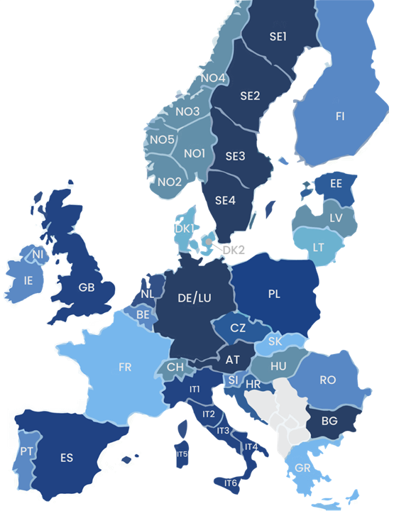
Figure 1: BZ in Europe

Source: Oliveira (2023)

Much of the existing research on BZ is focused around topics like network stability and optimal BZ configuration. Van den Bergh et al. (2016) quantify the impact of the number of BZs on electricity market outcomes of the Central European electricity system. Their findings suggest that a rising number of BZ is positively associated with network characteristics and a reduced risk of line overloads.

Breuer and Moser (2014) focus their research on the most efficient BZ. The authors fund that electric networks operate most efficiently if BZ borders reflect transmission bottlenecks. Since networks evolve over time Breuer and Moser suggest that BZ borders should be regularly readjusted to account for changes in network structure and the geographical allocation of electricity supply and demand. Nonetheless, this would have negative implications for planning security of market participants and harm investments into renewable generation capacity. Especially if there exist substantial price differences across BZ, changing the BZ borders would alter amortization periods.

Additionally, there exists a vivid discussion on the impact of BZ creation on the possible reallocation of energy intensive industries (Tagesschau, 2022; ENTSO-E, 2023). This is an especially fierce topic in Germany, where the surplus generating Northern states demand the creation of separate BZ. This would allow locals to benefit from previous investments into renewable generation capacity in form of reduced tariff rates and attract energy intensive industries to the otherwise agriculturally dominated North of Germany. Southern German states oppose this idea since they fear a reallocation of energy intensive industries to electricity abundant areas.

The effect of price divergence across BZ on investments in renewable energy technology has so far only been addressed in two studies. Hurta et al. (2022) estimate how the split of the German-Austrian-Luxembourgian BZ in 2018 has affected investments in battery storage systems, a popular tool to balance electricity supply variations from wind and solar generation. The authors use a flow model and data from 2 years before and after the BZ split for their estimation. Hurta et al.’s finding reveal that the higher electricity price volatility in Germany raises incentives for investments in battery storage systems the German-Luxembourgian relative to the Austrian BZ, since Austria relies mostly on hydropower and biofuels which can be adjusted to electricity consumption.

A limitation of Hurta et al.’s (2022) study is that actors that are located in the different BZ are even located in different countries. Therefore they do not face the same incentives schemes nor national policies, affecting their investment decisions. To circumvent this issue price divergence across BZ within a single country should be exploited. There currently exists merely one example for this type of study by Mauritzen (2023), who investigates the impact of electricity price divergence between Northern and Southern Norwegian BZ on pure-electric vehicle uptake. Similar to the Swedish case, Southern Norway has experienced electricity shortage and therefore a price increase compared to the North of the country. To further reduce the issue of underlying differences in investment propensity across BZ, Mauritzen merely considers municipalities close to the border between the high- and low-tariff BZs. It should be noted, that the paper lacks a clear motivation which municipalities should be part included in the border region.

Based on a simple difference and difference-in-difference approach, Mauritzen estimates that Southern Norwegian consumers were 2-5% less likely to invest in electric vehicles compared to their Northern Norwegian counterparts. This relatively modest impact can be accounted to the long-term nature of car purchases, the expectation that electric tariff differences will not persist in the long run, and the Norwegian ban of non-electric vehicle sales by 2025.

2.2 Photovoltaic generation

There are two main approaches to use sun light for energy generation, solar thermal and photovoltaic (PV) generation. This paper focuses on solar PV which "generate[s] electricity directly from light without emissions, noise, or vibration" (Panwar et al., 2011, p. 1516). PV generation requires sunlight needs to shine on solar modules made of semiconductor materials (Satpute et al., 2020; Lee and Ebong, 2017). Silicon-based crystalline solar modules are the by far the most popular, accounting for 95% of the world market (Andersson et al., 2021). Alternatives like thin-film applications are either made from amorphous silicon, copper indium gallium selenide, or cadmium telluride (Lee and Ebong, 2017). Despite lower material requirements and superior performance in highly insolated areas thin-film applications fail so far to compete with crystalline solar panels.

Apart from different types of solar modules, PV application can be divided into on- and off-grid applications (Andersson et al., 2021; da Silva et al., 2016). The latter are of major importance for electrification of islands, boats and remote areas. In developed countries such as Sweden, off-grid applications were especially popular during the early stages of PV adoption to electrify remote summer houses and boats. With increasing adoption of PV installations this generation mode lost popularity accounting for merely 0.4% of installed PV capacity in 2020 (Energimyndigheten, 2020).

On-grid applications can be further sub-divided into centralized and distributed generation. (Andersson et al., 2021). On-grid centralized PV generation is the most popular solar application, accounting for 55% of generation capacity worldwide in 2021 (IEA, 2022). Nonetheless, this generation mode is less popular in Europe especially in Sweden, were the share of distributed generation amounts to 94%. The main advantages of roof-mounted distributed PV applications over centralized plants are reduced transmission losses and improved network stability, since electricity is produced where it is consumed (Tamimi et al., 2013). Moreover, roof-mounted solar installation cause less social tension. Rising electricity prices have incentivized farmers to convert productive agricultural land into centralized solar farms creating a conflict between energy and food production and evoking resistance against centralized solar generation in Europe and the US (Katanich, 2023; Zinke, 2021; dos Santos Carstens and da Cunha, 2019).

A main concern regarding increased PV expansion are fluctuations in PV generation capacity, which is affected meteorological and seasonal fluctuations as well as topological aspects (Castillo et al., 2016). PV potential is greatest in the flat land areas close to the equator where seasonal changes in solar irradiation are least prominent. PV capacity is limited in mountainous areas where hills block solar irradiation in valleys most of the day. Further, PV capacity is reduced in areas with high occurrence of clouds and precipitation rates.

To balance electricity generated from solar sources over time, PV capacity need to be backed up with other forms of electric generation or coupled with storage facilities, typically in the form of batteries (Schmidt et al., 2016). The latter is of special importance in off-grid systems where solar energy serves as the sole energy source. However, integrated system including battery storage units are considerably more expensive limiting the ability of low-income households to afford solar installations. Additionally, batteries production is energy intensive based and disposal of toxic substances from battery production harms the environment (McManus, 2012).

2.3 Determinants of PV uptake

The selection of control variables for this study, requires and understanding of the main determinants of PV uptake. Determinants of PV uptake can be broadly categorized as geographic and socio-economic determinants which are discussed in separate subsections.

This review summarizes empirical findings from the US (Borenstein, 2017; Graziano and Gillingham, 2015), Japan (Zhang et al., 2011), Germany (Winter and Schlesewsky, 2019; Baginski and Weber, 2019), Belgium (Gautier and Jacqmin, 2020), Malta (Briguglio and Formosa, 2017), Brazil (Assunção and Schutze, 2017) and the UK (Balta-Ozkan et al., 2015).

2.3.1 Socio-economic factors

Findings of Balta-Ozkan et al. (2015), Borenstein (2017), Graziano and Gillingham (2015), Gautier and Jacqmin (2020), and Assunção and Schutze (2017) suggest that economic and financial incentives in form of electricity tariffs, disposable income, and unemployment are the main determinants of PV investments. Gautier and Jacqmin (2020) estimate that a marginal increase of the electric tariff rate by 0.01€ per kWh increase PV uptake by 8%. Furthermore, unemployment is associated with economic instability hampering the general propensity to invest. Briguglio and Formosa (2017) estimate that a 1% increase in the unemployment rate reduces the share of households with PV systems by 0.2%. Moreover, the financial situation of households has important implications for PV uptake. Borenstein (2017) and Winter and Schlesewsky (2019) detect a strong positive correlation between disposable household income and investment in solar generation since poor households frequently lack the financial means to cover initial investment costs. Since the initial investment costs are a major impediment to PV uptake, several governments offer assistance for households to cover initial investment costs (PV Magazine, 2022). This kind of subsidies exist among others in Austria and Cyprus.

Moreover, most European governments have implemented incentive schemes to promote renewable generation (PV Magazine, 2022; Bergek and Jacobsson, 2010). Feed-in-tariffs are the most popular way to promote investment in renewable generation capacity. Under this scheme, renewable electricity producers can consume their own electricity and sell their excess production on the electricity market at a fixed rate, which compensates them for generation costs but also provides them with an economic return.

The most popular incentive system in Scandinavia are tradable green certificates (TGC) (Bergek and Jacobsson, 2010; IEA, 2019; PV Magazine, 2022). As in countries with a feed-in tariff, renewable electricity producers can under a TGC scheme consume their self-generated electricity for free. Nonetheless, they do not receive a fixed amount of money per kWh inserted into the electric grid. Instead, investment costs are compensated through a the electricity market price plus a TGC, which is determined on a separate market. Governments create demand for TGC by setting requirements for providers to source a specified amount of electricity from renewable sources. To ensure an expansion of renewable generation, the minimum required share is regularly increased, raising the demand and thereby also the value of TGCs.

According to Bergek and Jacobsson (2010) and Fridolfsson and Tangerås (2013), TGC are an effective tool to raise the share of renewable generation for little tax funds. Nevertheless, TGC are problematic in regard to their effect on equity as well as technological development. Equity concerns arise since all producers of renewable electricity benefit from TGC including incumbent actors which do not face additional investment costs, providing them with access profit. Moreover, relying on a TGC therefore impedes the incorporation of novel electricity sources into a countries energy mix. Since the price of TGC is independent from the energy source, investors generate the greatest returns by investing in the technology with the lowest marginal costs. Relying on a TGC therefore impedes the incorporation of novel electricity sources into a countries energy mix.

Further socio-economic determinants of PV uptake include average age, environmental behavior and education levels which are however not considered as control variables in this study. Education is generally positively associated with PV uptake (Briguglio and Formosa, 2017; Balta-Ozkan et al., 2015). Nevertheless, since there also exists evidence for a correlation between household income and education level (Fischer and Strauss, 2021), the inclusion of both variables might bias estimation results. Empirical findings regarding the impact on age and environmental behavior point into different directions or lack statistical significance. Gautier and Jacqmin (2020) estimate higher PV uptake among older households in Wallonia, while it is most popular among young Maltese households (Briguglio and Formosa, 2017).

Environmental behavior reflected has been tested in several studies (Briguglio and Formosa, 2017; Gautier and Jacqmin, 2020; Baginski and Weber, 2019), but merely Zhang et al. (2011) find a significant positive effect on PV uptake. This can be explained by the observation period in the study by Zhang et al. (2011) which dates back to the early 2000s, when solar generation was generally not economically viable (IRENA, 2021). According to Palm (2020), the importance of environmental behavior diminishes as PV investments become financially attractive.

2.3.2 Geographic factors

The first of the geographic determinants is solar irradiation, which is affected by the distance to the equator, daytime, seasons and local weather conditions and topography (Yang et al., 2020; Castillo et al., 2016). While solar radiation increases the productivity of PV modules, empirical results regarding the relationship between solar irradiation and PV uptake are very mixed. Winter and Schlesewsky (2019) and Baginski and Weber (2019) detect a positive relationship between insolation rates and PV uptake in Germany. According to Baginski and Weber (2019) a 10% increase in irradiation translates to a 2.3% increase in installed potential. Nonetheless, Zhang et al. (2011) find no significant effect of irradiation in PV uptake in Japan, and in Brazil the relationship is even reversed (Assunção and Schutze, 2017).

Another factor that should be considered is the housing structure. Winter and Schlesewsky (2019) and Briguglio and Formosa (2017) identify roof space per capita as a key determinant of PV investment since PV installations are mainly worthwhile if they can cover the electricity consumption of the houses residents. This corresponds to the findings of Graziano and Gillingham (2015) whose findings suggest that PV uptake is highest in small and medium sized communities, which are especially in the US dominated by single family homes.

Access to complementary infrastructure and knowledge on alternative energy sources can be captured as neighborhood effects. According to by Balta-Ozkan et al. (2015) and Graziano and Gillingham (2015), neighborhood effects raise PV uptake in the short-run as greater awareness of the technology and the presence of solar installers increases households likeliness to invest in solar installations. However, this effect evaporates over time as market saturation is approached.

3 The Swedish case

Diffusion of solar generation is considered by several Swedish authorities as crucial for achieving Sweden’s climate targets and promote a transition towards entirely renewable electricity generation (Regeringskansliet, 2015; Miljödepartementet, 2019, 2020). This section provides background information on the history of solar generation and research in Sweden, as well as the establishment of separate BZ in the country.

3.1 The Swedish PV market

Off-grid solar generation emerged in Sweden already during the 1990s with the aim to electrify boats and remote cottages (Andersson et al., 2021). The government has supported this mode of solar generation actively with the establishment of the national development project SolEl which specifically targeted off-grid applications in 1995. From 2000 until SolEl’s discontinuation in 2018 it promoted even on-grid applications (Energimyndigheten, 2013).

Despite the emergence of solar generation in the mid-1990s, it should take two more decades until diffusion of solar generation occurred on the large scale (Energimyndigheten, 2023a; Andersson et al., 2021). As illustrated in figure 2, Sweden experienced exponential growth in PV installations since 2016 and does not display any signs of saturation. Between 2016 and 2022 total installed capacity increased by more than a factor of 17 reaching 2.38 GW by the end of 2022. This is far below the by Yang et al. (2020) estimated 65-84 GW of potential capacity of roof-mounted solar installations in Sweden.

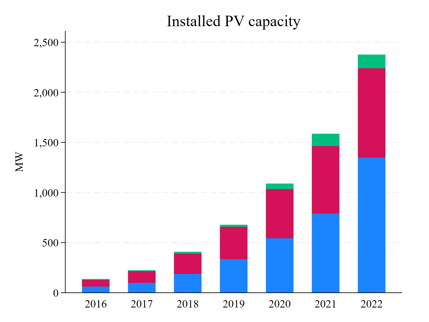
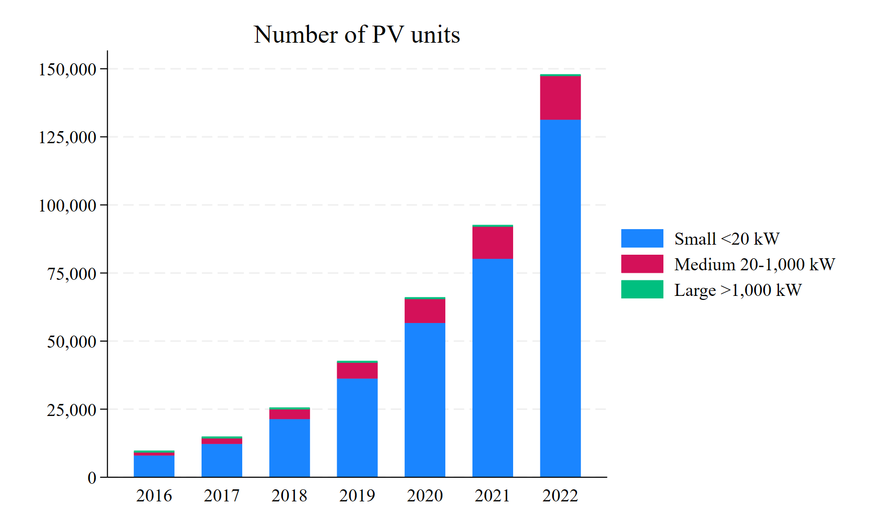
Figure 2: Grid connected PV installations by plant size, 2016-2022

Source: Energimyndigheten (2023a)

Nonetheless, the share of PV generation in Sweden remains low in an international comparison. The share of solar in total electricity generation between 2000 and 2022 is illustrated in Figure 3. While PV accounted for 1.36% of total electricity generation in Sweden, the share in Denmark was close to 6% and exceeded 10% in Germany and Spain. Only the neighboring Scandinavian countries Norway and Finland displayed significantly lower levels of PV generation amounting to merely 0.1% and 0.4%, respectively.

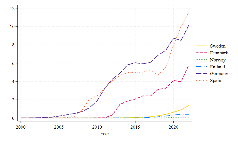
Figure 3: Share of solar PV in total electricity generation, 2000-2022 (%)

Source: Our World in data (2023c)

The comparably late investment in Sweden can be accounted to the countries geography but also financial incentives for investment in PV modules. First, Sweden is located between the 55°and 70°North, resulting in lower average radiation and higher seasonal fluctuations compared to countries with higher PV uptake (Castillo et al., 2016; SMHI, 2022).

Second, Sweden utilizes a TGC to promote renewable generation which primarily promotes the diffusion of mature technologies with low marginal costs (see section 2.3.1). As illustrated in figure 4 levelized generation costs of solar generation exceeded those of the cheapest renewable source hydropower by a factor of 10 in 2010. Since then the price of solar modules has fallen dramatically dropping to 0.06 USD per kWh in 2020, which exceeds the marginal costs of the cheapest renewable sources. Consequently PV diffusion was impeded until the mid-2010s, when PV installations became cost competitive with alternative energy carriers (Bergek and Jacobsson, 2010; IEA, 2019; PV Magazine, 2022). PV generation is not the only energy technology impeded by the TGC. Wind power is the second most important renewable energy source in Sweden accounting for 17% of total electricity generation in Sweden but its diffusion was delayed until 2010 when it became cost competitive with alternative technologies (IEA, 2023; Bergek, 2010). Consequently, the TGC is likely to impede the diffusion of energy carriers developed in the future.

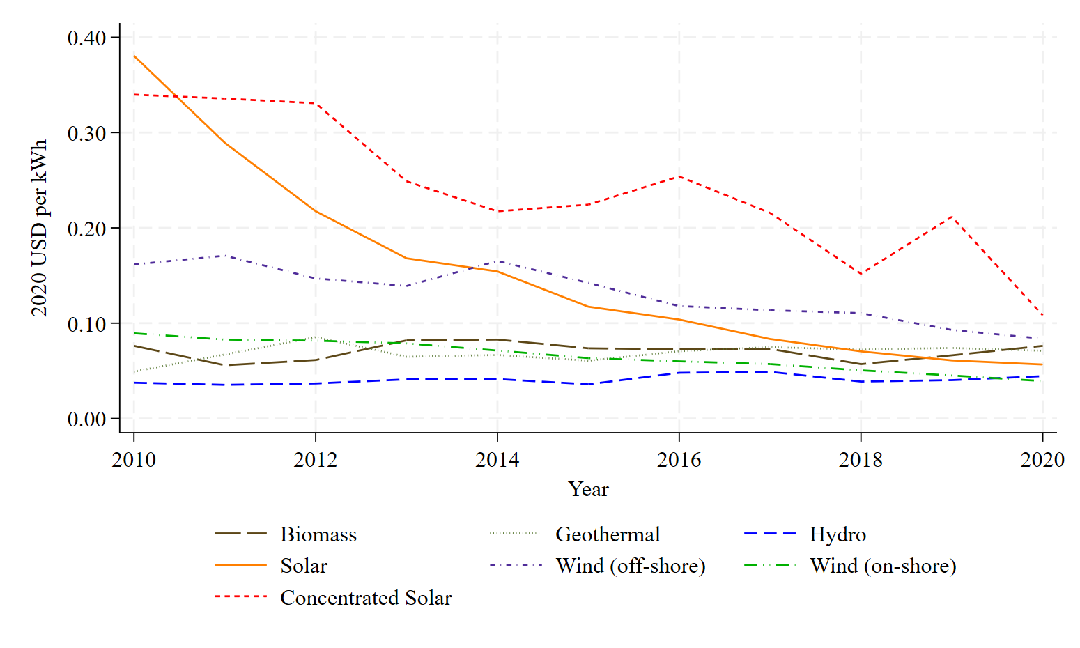
Figure 4: Levelized renewable energy generation costs, 2010-2020 (2020 USD/kWh)

Source: IRENA (2021)

Third, while the first government subsidy for PV installations was very generous covering 70% of initial investment costs, wide-spread was impeded since it merely targeted public actors until 2009 (Andersson et al., 2021). In 2009, this scheme was extended to all on-grid distributed generation, promoting PV investment throughout the population. Together with falling marginal costs PV capacity increased by 53% annually but contributed still only for 0.1% of total generation capacity by 2015. With falling marginal costs and rising PV uptake over recent years, investment subsidies have undergone additional reforms under recent years and became overall less generous. Since 2019, it is limited to 20% of installation costs or 1.2 million SEK per plant (Swedish Government, 2020). Additionally, the government covered 60% of initial investment costs for storage units. In December 2020 subsidies for initial investment costs were discontinued and fully replaced with tax exemptions, amounting to 20% and 50% for PV modules and storage systems, respectively (Energimyndigheten, 2023b).

Fourth, Sweden lacks linkages between PV research and production. Since the emergence of solar research in the 1980s, Swedish PV research in focused on thin-film PV modules panels, an alternative to the dominant crystalline solar panels (Andersson et al., 2021). While the first PV company Solibro specialized on this technology, other PV companies that started production in the early 2000s focused on the more popular crystalline modules instead (Energimyndigheten, 2020). The situation deteriorated when competition from China resulted in the collapse of the European PV industry in the late 2010s. Solar cell production literally disappeared in Sweden by 2016. Since 2019, two companies started to produce thin-film PV modules. However, their combined production of 1.2MW is by far insufficient to cover the demand for new solar installations in Sweden which exceeded 400MW in the same year (Energimyndigheten, 2020, 2023a).

3.2 Electricity price divergence

Sweden was divided into four BZ in 2011, following a directive from the EU with the purpose to prevent sudden export stops of Swedish electricity to other EU members Swedish Energy Markets Inspectorate (2022). The Swedish BZ configuration is illustrated in figure 5. BZ do not necessarily follow municipality borders. In fact 25 municipalities marked in dark blue are located in multiple BZ allowing for tariff divergence within a single municipality. A complete list over the Swedish municipalities and the tariff area they belong to can be found in table LABEL:tab:municipality_list in the appendix.

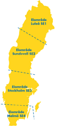
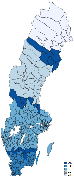
Figure 5: Electric tariff areas

Source: SHE (2022) and Svenska Kraftnät (2022)

By creating different tariff areas policy makers opened even the doors for differentiated electricity prices across tariff areas. Electricity prices between 2015 and 2022 are illustrated in figure 6. While electricity prices fluctuated over time, divergence across BZ emerged only in 2020 when electricity shortages in Southern Sweden drove up electricity prices in BZ SE3 and SE4. Creating the conditions for a natural experiment on solar PV uptake along the border of the high- and low-tariff BZ SE3 and SE2. According to Vattenfall (2023), electricity prices differences reached a record of a factor of 12 in August 2022. Since mid-2022 electricity prices started to converge as prices in the Northern BZ SE1 and SE2 increased.

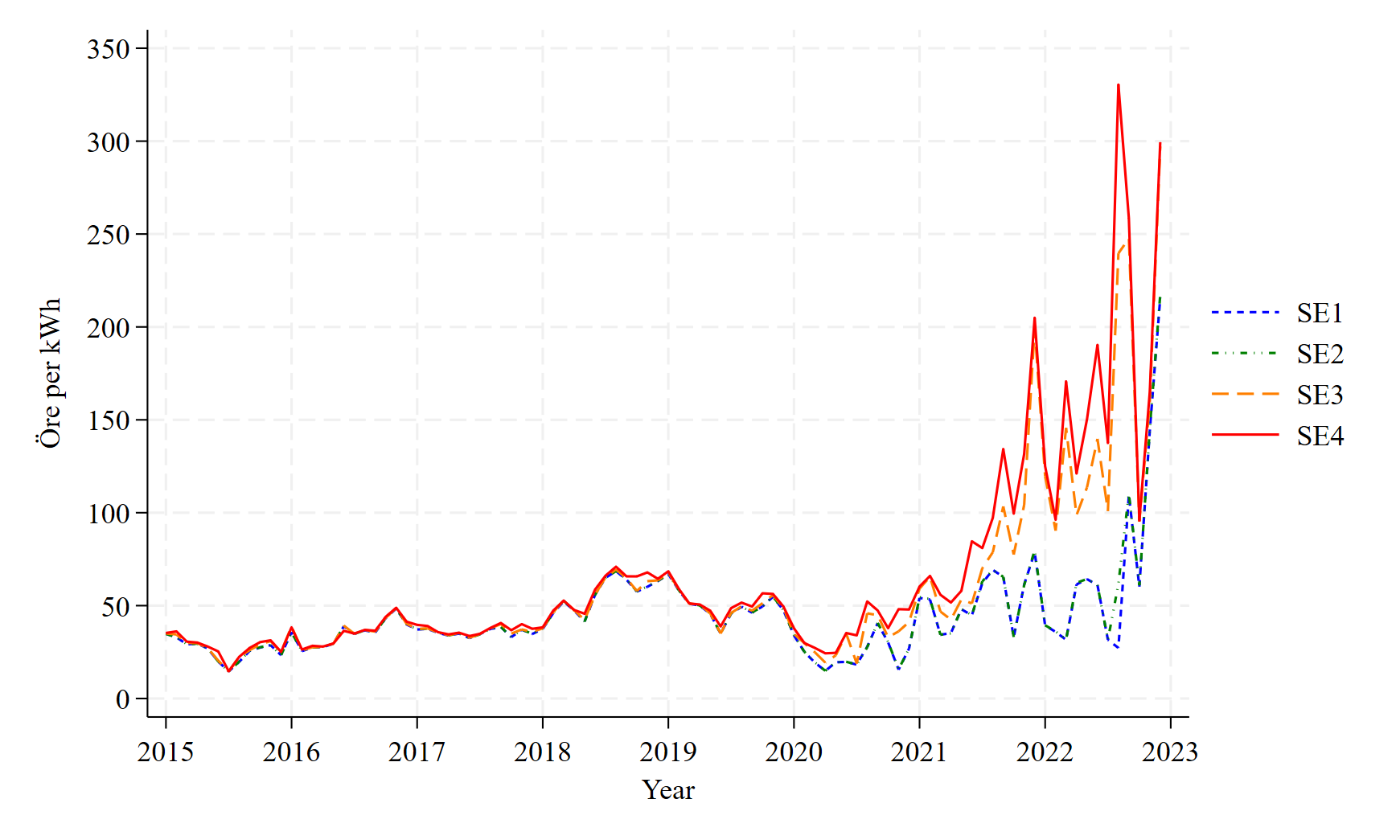
Figure 6: Floating electricity tariff by BZ, 2015-2022 (öre/kWh)

Source: Vattenfall (2023)

Installed PV capacity per BZ is illustrated in figure 7. PV uptake in Sweden is highest in the Southern most BZ SE4 and lowest in SE1 in the far North. While this corresponds to the higher productivity of PV installations in the South of the country the gap has widened since 2020, when rising electricity prices drove up demand for PV installations in the Southern BZ. The aim of this study is to isolate the effect of electric tariff divergence on PV uptake from other factors impeding PV uptake in Northern Sweden.

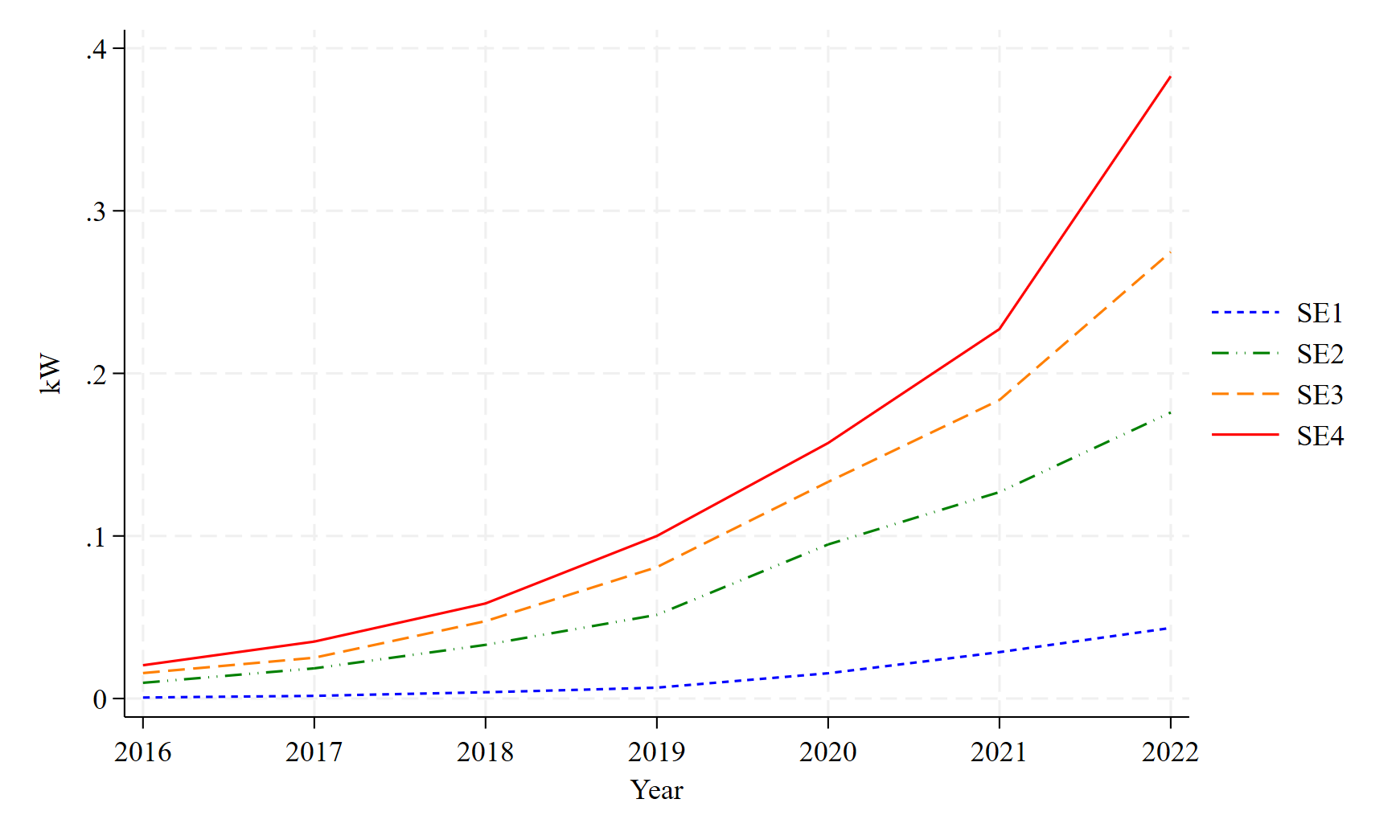
Figure 7: Installed PV capacity per capita by BZ, 2016-2022 (kW)

Source: Energimyndigheten (2023a)

4 Data

To estimate the effect of price divergence across BZ on PV adoption, a balanced panel data set is created containing a total of 2,030 annual observations for all 290 Swedish municipalities between 2016 and 2022.

The choice of the observation period is driven by data availability of the outcome variable installed PV capacity is provided by Energimyndigheten (2023a) on the municipality level only from 2016 onwards. It should be noted that only small- and medium-sized on-grid installations with a maximum capacity of 1 MW are considered. This is motivated by the fact that these account for 95% of the solar PV market in Sweden, and that there existed merely 11 PV plants with a capacity above 1 MW which accounted for less than 3% of solar capacity by the end of 2019 (Energimyndigheten, 2020, 2023a).

Moreover, installed PV capacity is measured in per capita terms to account for the vast differences in population size across Swedish municipalities which has significant implications for electricity demand as these two factors are positively correlated and demand for PV systems (Assunção and Schutze, 2017). In 2021, Swedish population by municipality varied from merely 2,385 residents in Bjurholm (Västerbotten) to approximately 1 million in Stockholm (SCB, 2022).

Since the main aim of this paper is to estimate how price divergence across BZ affects PV uptake, the treatment status is determined by a dummy variable which takes the value 1 if a municipality is located in a low-tariff BZ SE1 or SE2. The seven municipalities that cannot clearly be assigned to the low- or high-tariff areas are excluded from the sample. The treatment status of all municipalities is documented in table LABEL:tab:municipality_list.

Additionally, solar irradiation, unemployment rates, disposable income, and the housing structure are included as control variables. Irradiation data is sourced from the Strång database which is provided by the Swedish Meteorological and Hydrological Institute (SMHI, 2023). Data from Strång can be extracted for every single geographic location in Scandinavia since 1999. For this paper daily global radiation data is extracted for each communities central settlement (centralort) over the period 2010-2015.

The obtained irradiation data is used to create two variables. Average radiation refers simply to the average daily radiation between 2010-2015. Radiation variation is added to account for seasonal variation in sunlight hours which reduces incentives for the adoption of PV systems in areas with large seasonal variations (Castillo et al., 2016). It is calculated by the average radiation per month over the 6-year period and then dividing the maximum by the minimum monthly radiation. The value of both variables is fixed within municipalities over the observation period.

Information on disposable income, population size, and the housing structure of Swedish municipalities is retrieved from the SCB (2022). Annual observations of disposable income are reported in per capita terms for all Swedish municipalities from 2000 onwards.

Housing structure refers to the share of small houses. The SCB (2022) distinguishes between small houses (småhus), with 1-2 housing units, apartment buildings (flerbostadshus) with 3 or more housing units, other houses (övriga hus) which do not exclusively serve for housing purpose and special housing (specialbostäder) like student housing and retirement homes. According to Öhrlund et al. (2020) it is important to consider the housing structure when studying solar PV uptake in Sweden. PV diffusion among residents of housing cooperatives and rental buildings is slowed down or prevented since they must align their investment decisions. Moreover, roof area per inhabitant is smaller compared to single family houses reducing the attractiveness of PV investments (Winter and Schlesewsky, 2019).

The unemployment data is merely available at the regional level (län). The data measures unemployment as the proportion of people in the labor force aged 15-74 years who are unemployed on the regional level. Important to note is that unemployment data is missing for Gotland after 2019. It is assumed that unemployment stayed constant at the 2019-level of 6% after this.

To avoid the risk of bad controls observations of the time-variant control variables are assigned to the following year. Hence, the controls for the 2016 observations are measured in 2015. This is motivated by the risk of bad control variables. If control variables are determined simultaneously or after the outcome variable the value of the control variable might be determined by the outcome variable instead (Angrist and Pischke, 2009, p.47-48).

Table 1: Descriptive statistics

Variable	Observations	Unit	Mean	Std. dev.	Min	Max
Installed capacity	2,030	kW	0.105	0.114	0	0.95
per capita
Average radiation	2,030	kWh/m2	1,240	96	931	1,437
Radiation variation	2,030		42.3	71.7	15.7	764.6
Disposable income	2,030	SEK	210,002	25,028	165,000	463,000
Unemployment	2,030	%	7.0	1.6	4.3	11.5
Housing structure	2,030	%	61.9	0.1	1.4	90.2

Descriptive statistics are presented in table 1. There exists considerable variation in outcome and control variables across municipalities. While average installed capacity amounted to 0.1 kW per capita over the entire observation period, the maximum installed capacity of 0.95 kW per capita was reported in Borgholm (Kalmar) while three municipalities in Norbotten had not even a single PV installation by 2020.

Another variable that stands out are radiation levels, which were highest in Karlskrona (Blekinge) and lowest in Kiruna (Norbotten), amounting to 1,437 and 931 kWh/m², respectively. Kiruna even has the highest radiation variation of 765, due to its location North of the Arctic circle (SMHI, 2022).

4.1 The three border regions

As discussed previously, PV uptake across BZ differs substantially across Sweden. This can partly be accounted to underlying differences in control variables, in particular solar radiation levels which are significantly lower in the low-tariff BZ in Northern Sweden. Simply comparing BZ to one another would therefore most likely not produce any meaningful results.

Instead, the analysis focuses on the border region between the low- and high-tariff BZ SE2 and SE3. A similar approach has been applied by Mauritzen (2023) to study electric vehicle uptake in Norway. Nonetheless, selection criteria for including municipalities in the border region remain somewhat unclear apart from the fact that neither of them contains any major cities.

In the following analysis three different definitions of the BZ border are considered, defined by their geographical difference from the border between the low- and high-tariff BZ. The resulting tariff areas are presented in figure 8. A list over the municipalities included in the different border regions is included in table LABEL:tab:municipality_list in the appendix.

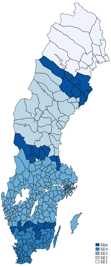
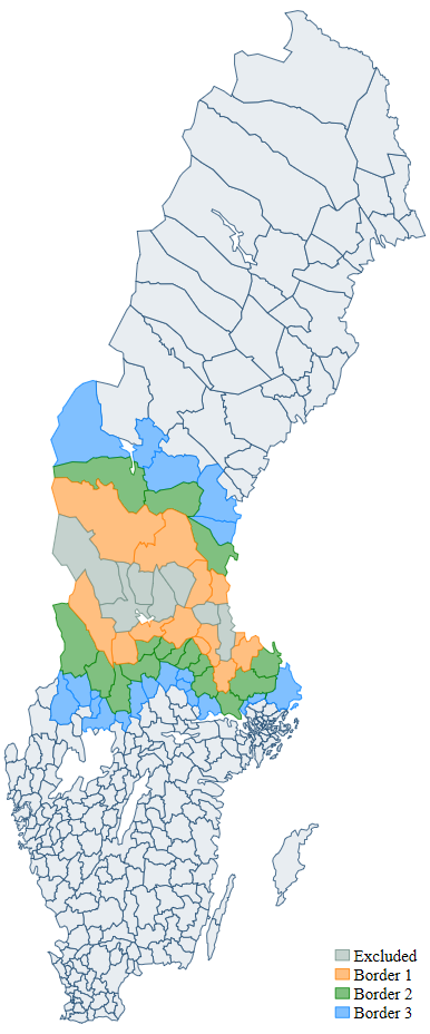
Figure 8: Border regions

Border 1 refers to municipalities at the BZ border between electricity tariff areas SE2 and SE3 or those municipalities that are part of both areas and therefore excluded from the analysis. Border 2 comprises all municipalities included in border 1 plus municipalities that have a direct border with any of the municipalities in the border 1 group. Similarly, border 3 includes all border 2 municipalities as well as those that have a direct border with them.

The data on outcome and control variables for each border region is calculated by taking the average of outcome and control variables. Since municipalities located in the high- and low-tariff areas are considered separately, values for six different border regions are calculated. The three Northern BZ border regions are of main interest for the following analysis.

5 Synthetic Control Method

The Synthetic Control Method (SCM) has been developed by Abadie and Gardeazabal (2003) as an alternative to time-series analysis, comparative case studies, and difference-in-difference (DiD) approaches which are commonly used to quantify the effects of policy interventions by(Card, 1990; Richardson and Troost, 2009).

To estimate the actual treatment effect the outcomes for the affected unit should be compared in the presence and absence of treatment, which refers here to the location of a municipality in the low-tariff BZ. The problem however is that a municipality cannot simultaneously face high- and low-tariff prices. Hence, it is necessary to model the counterfactual outcome, the one that cannot be observed with help of econometric techniques (Billmeier and Nannicini, 2013; Abadie and Gardeazabal, 2003; Abadie, 2021).

The synthetic control group (SCG) is defined as the "weighted average of the units in the donor pool" (Abadie, 2021, p.395). The donor pool consists of non-treated comparison units. The treated unit in this study is the Northern BZ border located in the low-tariff BZ SE2, while the donor pool consists of all municipalities in the high tariff areas SE3 and SE4.

$$\mathrm{Y^{S}_{it,T=0}=\sum^{J+1}_{j=2}w_{j}Y_{jt,T=0}}$$ (1)

The composition of the SCG $Y^{S}$ of the treated unit i is formally presented in equation 1. Observations from the donor pool j are assigned weights w to minimize the difference between the pre-treatment outcomes of the treated and the SCG, presented in equation 1.

Weights are assigned based on a set of predictor variables, whose selection is similar to the selection of control variables in other econometric models a fundamental component of the estimation process Abadie (2021). Predictor variables consist of pre-intervention values of the outcome variable combined with variables that potentially affect outcome levels. In this study the predictor variables consist of three pre-treatment values of the outcome variables installed PV capacity per capita in 2016, 2018, and 2020, average radiation, radiation variation, disposable income, the share of small houses, and the unemployment rate.

The SCM rests on two main assumptions. First, according to the non-interference assumption the treatment status of treated unit i is independent from donor units j. Second weights are restricted to non-negative values and must sum up to one. This ensures a donor pool consisting of relatively few comparison units (Abadie and Gardeazabal, 2003; Abadie, 2021).

The Synthetic control approach has become popular over recent years since it has several advantages over other comparative case study designs. First, SCM are particularly suited when only few control units are available or when outcomes for aggregate units such as municipalities or countries are estimated (Abadie et al., 2010, 2015; Abadie, 2021).Abadie et al. (2015) apply SCM to estimate the effect of reunification on West German GDP per capita, while Dube and Zipperer (2015) estimate the effect of minimum wage policies across US states.

Second, SCM offers in difference to comparative case studies and DiD a formal and entirely data driven selection procedure to identify control units. Thereby SCM limits researchers’ possibilities to bias estimation results through p-hacking or specific searches (Billmeier and Nannicini, 2013). Moreover, SCM can even account for time varying unobservable confounders.

Third, the evaluation of the fit of the SCM model is very transparent since outcome values for the treated unit and its SCG should ideally be identical during the pre-treatment period (Abadie et al., 2010; Abadie, 2021; Billmeier and Nannicini, 2013).

Finally, the condition of non-negative weights summing up to one prevents extrapolation and simplifies interpretation of estimation results (Abadie et al., 2010; Abadie, 2021; Billmeier and Nannicini, 2013).

Despite the numerous advantages of the SCM, Abadie (2021) identifies a number of contextual and data requirements that need to be considered when applying SCM. First, SCM should not be applied if the treated unit is an outlier. This would for occur if a outcome or predictor value would lie outside the range of all potential control variables. Second, high volatility of outcomes can negatively affect the detectability of the treatment effect. Third, units that suffered from large idiosyncratic shocks should be eliminated from the donor pool. This would be the case if for example solar panels were destroyed by a storm or if a large-scale solar project was realized in one of the municipalities, resulting in a massive change in the outcome variable installed PV capacity per capita. Fourth, the validity of the non-interference assumption might be violated in the presence of spill-over effects. The treatment affect might be attenuated if the treatment status of unit i, would affect geographically proximate areas. Fifth, the treatment should not be foreseeable by policy makers. Finally, since the SCG is a weighted sample of control units, substantial differences between its members might be averaged away, reducing the representativity of the treated unit. Whether this is the case can be checked by comparing the predictor balance of the SCG members.

Apart from contextual requirements, the application of synthetic controls requires aggregate data. Micro-level data can be used to obtain outcome or predictor values on the desired aggregate level. Moreover, pre- and post-intervention periods must be sufficiently long. In case that pre-treatment periods are too short, there exists the risk of over-fitting, while limited availability of post-intervention data might not capture the treatment effect to its full extent.

6 Results

This section presents the regression results from the SCM estimations separately for the three definitions of the BZ border region. Installed PV capacity for the the border 1-3 and its SCGs are illustrated in figure 9, 10, and 11, respectively. The SCG composition SCG is documented in table 2.

Table 2: Synthetic control group composition

Border 1			Border 2			Border 3
Sandviken	47%		Gagnef	38%		Gagnef	36%
Gagnef	37%		Vansbro	27%		Vansbro	30%
Borlänge	10%		Norberg	19%		Borlänge	12%
Vansbro	6%		Borlänge	12%		Falun	11%
			Sandviken	4%		Norberg	7%
						Leksand	4%

The municipalities used to construct the control groups are all located in geographical proximity of the BZ border between SE2 and SE3. All SCGs are sparse since they consist of a maximum of six out of the 234 municipalities included in the donor pool. Three municipalities are present in all SCGs, which can be accounted to the fact that border region contain by definition the same municipalities located in close proximities of the BZ border.

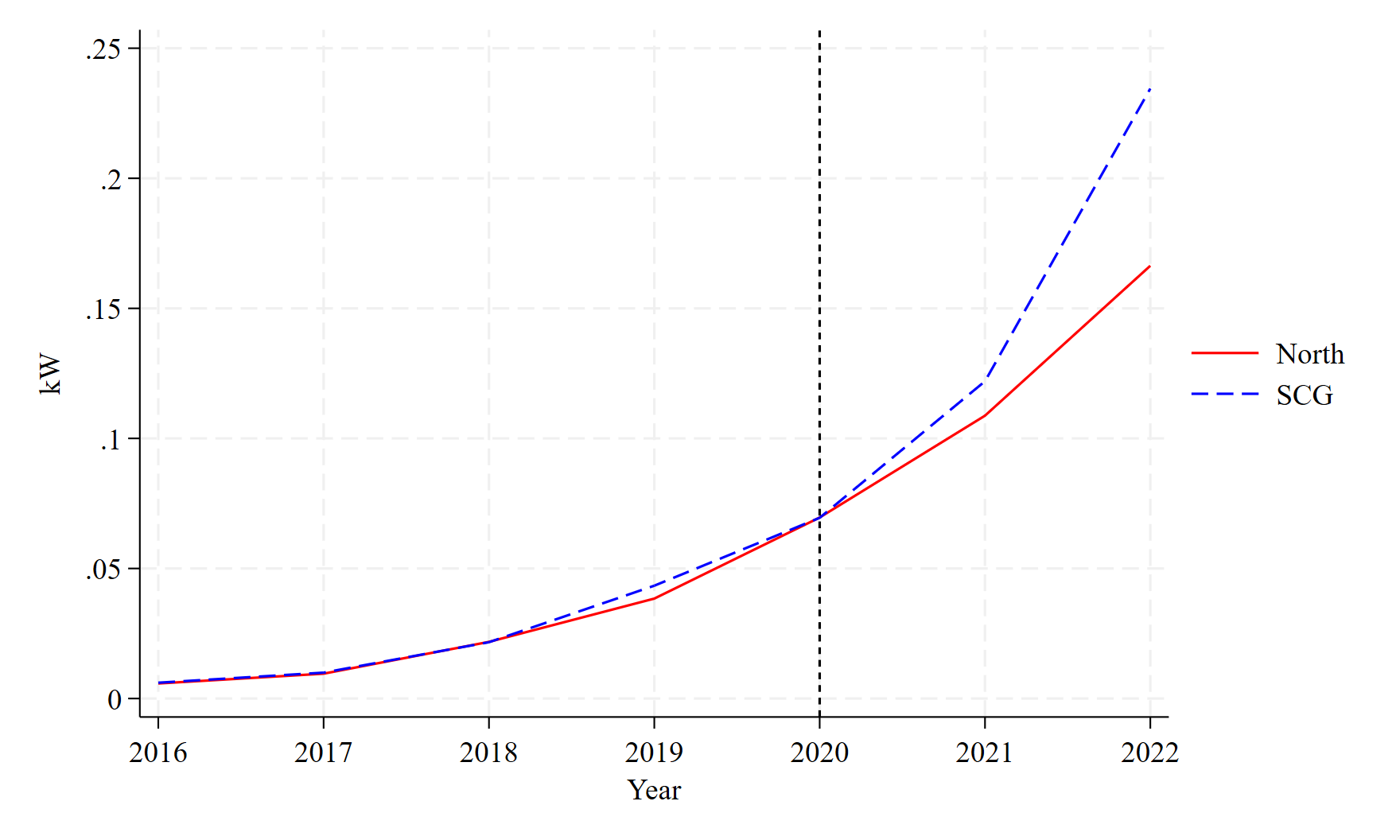
Figure 9: Border 1, 2016-2022 (kW per capita)

Figures 9, 10, and 11 reveal that outcome levels for the border and control regions are closely fitted during the pre-treatment period. A sizable deviation in outcome levels can only be observed in 2019 for border region 1 and 2, amounting to 12.9% and 12.4% in relative terms.

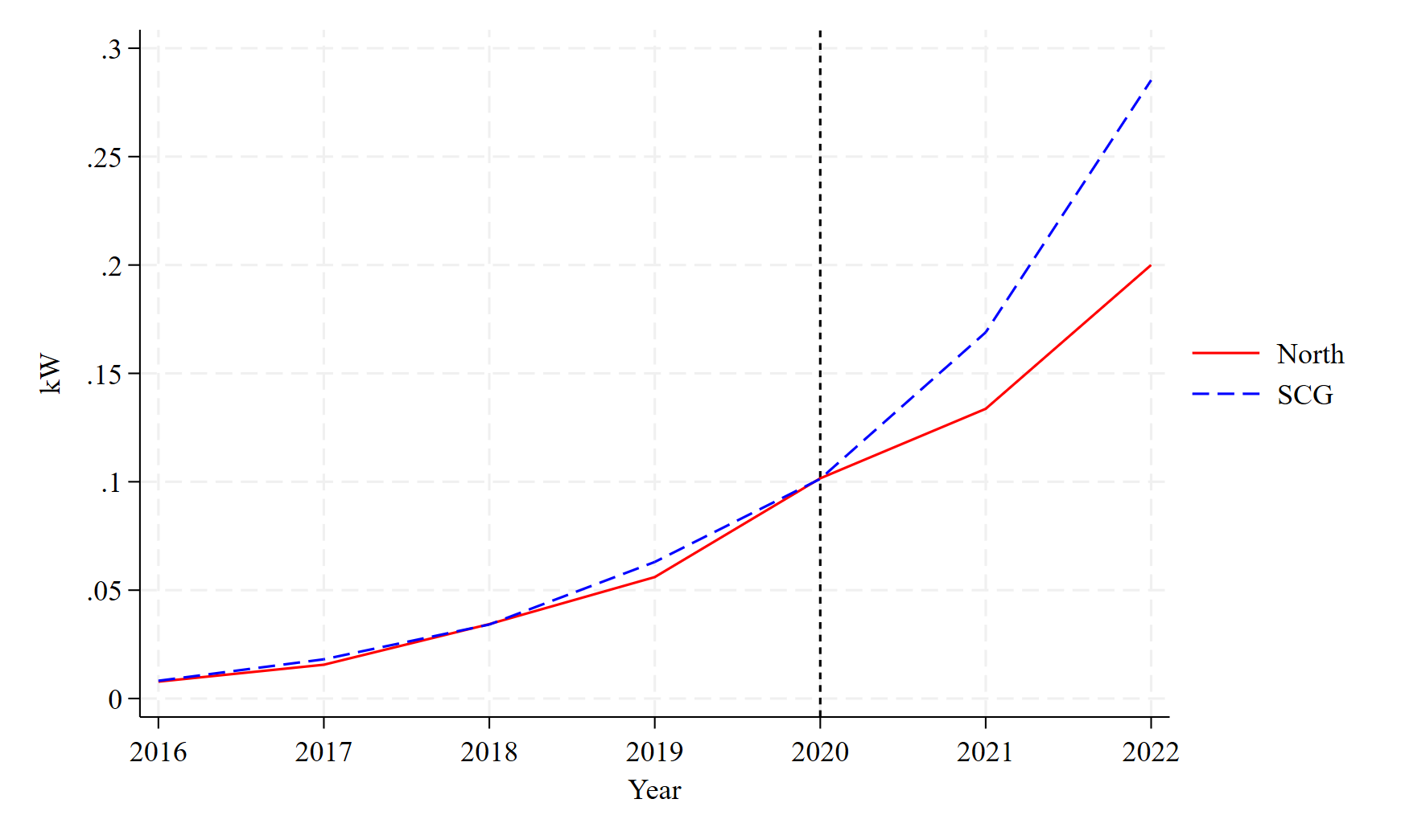
Figure 10: Border 2, 2016-2022 (kW per capita)

After 2020 PV uptake in the low-tariff border regions diverges clearly from its SCG. The size of the absolute and relative treatment effect are presented in table 3. The effect of electric tariff divergence arises already in 2021, but remains with 0.01 kW or 12.2% insignificant for border 1, as deviations in pre-treatment levels are similar to the size of the 2021-estimate. For border 2 and 3 the effect size amounts to 0.04 kW or 22.4-22.6% a single year after the emergence of electric tariff divergence in Sweden. A statistically and economically sizeable effect.

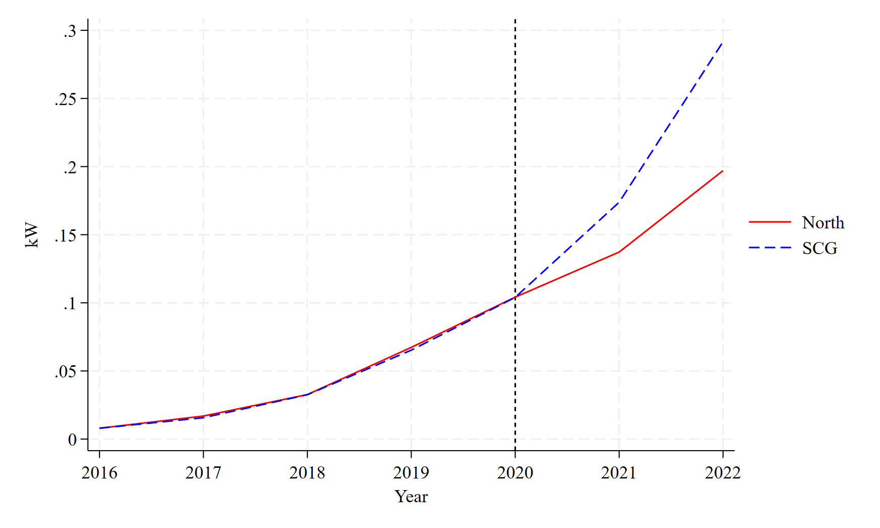
Figure 11: Border 3, 2016-2022 (kW per capita)

This situation changes when the data from 2022 is included. Two year after the start of treatment, the total effect rises to 0.07 kW and 0.09 kW, for border region 1 and both border regions 2 and 3, respectively. The size of relative effect size exceeds 40% for all border regions but is with 48% largest for border 3.

Table 3: Absolute and relative treatment effect

	Border 1	Border 2	Border 3
Absolute (kW)
2020	0.00	0.00	0.00
2021	-0.01	-0.04	-0.04
2022	-0.07	-0.09	-0.09
Relative (%)
2020	0.02	0.02	0.02
2021	-12.2	-26.4	-26.6
2022	-40.9	-42.6	-48.0

Important when evaluating the representativity of the SCG, is to compare the predictor balance of the SCG to the treated unit. These figures are compared in table 4 in absolute terms. Differences are most pronounced in radiation variation and increase when the border definition is widened. Differences in radiation variation are greatest for border 3 and its SCG amounting to a factor of 15 or 34.4%. Nonetheless, this is unavoidable due to the geographic location of the BZ border. It is not considered as a serious issue here since differences in average radiation levels are far less pronounces amounting to a maximum of 46 kWh per $m^{2}$ or 4.1%.

Table 4: Predictor balance

	Border 1		Border 2		Border 3
	Treated	SCG	Treated	SCG	Treated	SCG
Income	194063	193843	194429	194750	195729	196843
Radiation	1155	1184	1127	1164	1118	1164
Radiation variation	36	28	39	28	43	28
Unemployment	9%	8%	8%	8%	8%	7%
Small houses	64%	67%	66%	72%	63%	73%
Capacity 2016	0.006	0.006	0.008	0.008	0.008	0.008
Capacity 2018	0.022	0.022	0.034	0.034	0.033	0.033
Capacity 2020	0.070	0.069	0.102	0.101	0.104	0.104

Apart from radiation variation, differences between the border region and their SCGs is greatest in terms of the unemployment rate. For border 2, the unemployment rate in the North exceeds that of the SCG by 0.51 percentage points which corresponds to a relative difference of 6.32%.

7 Discussion

This section discusses the implication of the estimation results for future PV expansion in Sweden and other European countries. Moreover, the use of SCM is critically evaluated and the results are compared to an alternative DiD estimation. Finally, the suitability of the alternative border region definitions is assessed to create a benchmark for future studies.

7.1 Implications of the empirical findings

The main finding of the study is that electricity price divergence since 2020 reduces PV uptake in the low-tariff BZ in Northern Sweden by 40.9% to 48% depending on the border region specification. This supports empirical findings that identify economic incentives as the main determinant of PV uptake in Sweden and elsewhere (Palm, 2020; Gautier and Jacqmin, 2020; Balta-Ozkan et al., 2015; Borenstein, 2017; Assunção and Schutze, 2017). Moreover, the study supports previous findings on the efficiency of BZs as an instrument to direct renewable energy investments towards areas with greatest imbalances in electricity supply and demand (ENTSO-E, 2023; Hurta et al., 2022).

Positive effects on the supply balance are contrasted by the rapid divergence in PV uptake across the country, which could harm countries prospects to realize their full PV potential and undergo a successful transition towards renewable generation. This is less concerning in Sweden with overall low PV uptake in an international comparison, a 70% contribution of renewable sources to total electricity generation, and most of the low-tariff BZ being deemed technically unsuitable for an expansion of PV generation (IEA, 2023; Castillo et al., 2016; SMHI, 2022). Nonetheless, it should be considered in countries with low initial contribution of PV and overall renewable electricity generation such as the Czech Republic, PV investments would only be incentivized in the high-tariff BZ (Our World in data, 2023c, b). Similarly, existing inequalities in PV uptake would be reinforced in countries like Germany. Southern German states already display the highest levels of PV penetration and are expected to face the highest electric tariff rates if separate BZ are created. Meanwhile, incentives for PV investments in Northern Germany with the largest remaining potential would deteriorate along with the prospects for a successful German energy transition (Winter and Schlesewsky, 2019; Tagesschau, 2022; ENTSO-E, 2023).

Short-run imbalances in PV investments might become persistent in the long-run since their exist limitation to regional catch-up potential. Europe is currently facing a severe shortage of qualified solar installers. Despite massive demand, uninstalled PV modules are being stockpiled throughout the continent (Bloomberg, 2022; Blom Westergren, 2022). Even if this issue was addressed, the problem remains that Europe imports the vast majority of its solar modules from China. Any kind of trade disruptions could therefore harm both, a successful energy transition and electricity supply security in Europe (Hancock, 2023).

Furthermore, increased PV investments in high-tariff BZ could compromise grid stability due to the volatility of PV generation (Castillo et al., 2016). Increasing reliance on solar generation would require additional investment in grid infrastructure and storage capacity, which has resulted in multiple confrontations between locals and public authorities in the past (Hurta et al., 2022; Schmidt et al., 2016). Local resistance has been so severe that governments in Sweden and Germany have discontinued funding and implemented laws impeding the realization of large scale energy projects to win over voters (Tidöavtalet, 2022; Stede and May, 2019).

Nonetheless, BZ creation might enact sufficient pressure on policy makers to raise community acceptance and remove legal impediments against energy infrastructure projects in general. According to Hogan et al. (2022) and Sena et al. (2016) the majority of local resistance arises from the lack of financial returns from energy projects and their inability to influence the planning process. Both issues can be tackled by granting local communities full or co-ownership of the energy projects. Greater involvement of locals in the decision making process would be of special importance if separate BZ are created in since the Southern part of the country faces the biggest electricity shortage and is home to the fiercest opponents of energy projects.

7.2 Is the use of synthetic controls justified?

While the estimation results are economically and statistically significant, it must be evaluated whether the use of the SCM is appropriate for the present study. First of all, contextual aspects are assessed. The validity of this study would be compromised if policy makers were able to foresee the impact of price divergence on PV uptake when BZ were created in 2011 (Billmeier and Nannicini, 2013). This seems like an unlikely scenario since solar generation contributed back then less than 0.01% to total electricity generation in Sweden (Our World in data, 2023c). Moreover, electricity price divergence occurred merely in 2020, one decade after BZ were first created (Energimyndigheten, 2023a; Vattenfall, 2023). Finally, price divergence is partly driven by forces outside of Sweden namely the European electricity market integration and the absence of BZ in Germany combined with high demand, which incentivize exports even when electricity is in low supply in SE3 and SE4 (Dagens industri, 2023).

The temporal distance between investment decision and realization projects might be a challenge in this study, since data is only available two years after the start of treatment. Moreover, the lack of solar installers that affects the entire EU is also apparent in Sweden (Blom Westergren, 2022). Waiting times for PV installations amount currently to about four month but vary across municipalities. The unequal access to PV installers could bias the estimation results in case that the access differs between the Northern BZ border and its SCG. The treatment effect might be overemphasized if access to solar installers was better among the SCG, while superior excess in the Northern BZ border would lead to its attenuation.

Apart from contextual requirements, it must be ensured that the regression data is suited for the application of SCM. Therefore, a number of statistical tests have been performed. First, neither outcome nor control variables should lie outside the range of observations from the donor pool during the pre-treatment period. Moreover, results are most significant when outcomes in the post-treatment period lie outside the range of outcome levels of the donor pool. Whether this is the case can be accessed with help of a permutation distribution which displays the maximum and minimum levels of PV uptake among all municipalities included in the donor pool compared to the three border regions (Abadie, 2021).

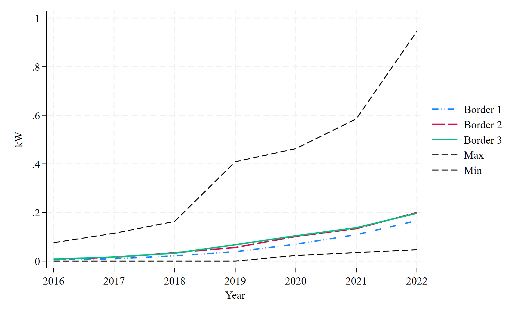
Figure 12: Permutation distribution, 2016-2022 (kW per capita)

The permutation of the outcome variable installed PV capacity per capita is illustrated in figure 12. The dashed lines indicate the maximum and minimum values from the donor pool. All border regions fulfill the condition that their outcome value are contained within the range of the donor pool. Nonetheless, the outcomes of the border regions remain within the range of outcomes in the high-price area casting some doubt on the significance of the estimation results, since there exist municipalities in the high-tariff areas with considerably lower levels of PV uptake.

Placebo tests are conducted to check for significant deviation in outcome levels between the border regions and their SCGs before actual treatment starts in 2020. For this purpose, the SCM regressions are repeated assuming the same placebo treatment period in 2018, with one less pre-treatment value in 2020.

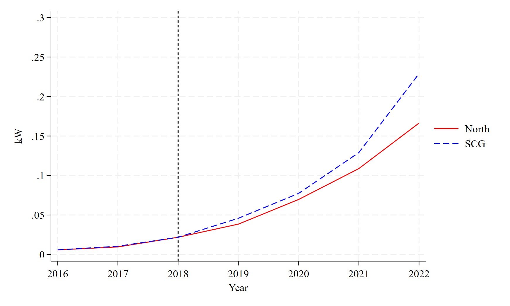
Figure 13: SCG - Placebo test Border 1, 2016-2022 (kW)

The placebo test results are presented in figures 13, 14, and 15. Significant deviation between the Norther BZ border and its SCG arises only after 2020. This applies especially to border region 2 and 3, where the outcome of the treated unit exceeds that of its SCG. This supports the hypothesis that price divergence from 2022 onwards is the main driving force for deviations in PV uptake across BZ.

Finally, there exists a risk that the SCG does not properly represent the treatment unit. This problem would arise if there exist large variations in outcome and control variables between the members of the SCG, which would simply be averaged away due to the choice of the estimation method (Abadie, 2021). To investigate this issue, values of outcome and control variables of individual members of the SCGs are presented in table 6. All values of the control variables are the observations for 2016, while the value of the outcome variable is observed at three points in time, 2016, 2018, and 2020, which are also used to construct the SCGs.

Table 6 reveals that there exist significant variation within the SCGs regarding installed PV potential and the housing structure in the municipalities. For all SCGs the share of small houses varies by a factor of two or 45 percentage points. This has sere effects on incentives and potential for PV capacity which is especially visible in the of Borlänge, which is part of all SCGs and has both the lowest share of small houses and PV capacity installed.

7.3 Alternative estimation

The only other paper that uses electricity price divergence across BZ in Scandinavia as a natural experiment to estimate its effect on renewable energy technology investments was conducted by Mauritzen (2023), based on a DiD approach. The study’s results are somewhat conflicting to ours since Mauritzen only detects an economically insignificant effect. While this might simply be driven by the different nature of the energy technologies or the country specific context, alternative DiD estimation of PV uptake in Sweden are presented in the appendix to investigate whether our results are robust to the choice of the estimation methods.

As presented in table 7, the only statistically significant result are reported for border 3 when control variables are included. This effect is however very small in magnitude amounting to no more than 0.003 kW, corresponding to approximately 1.5% of installed PV capacity in border 3 in 2022.

Furthermore, DiD are deemed unsuitable to investigate PV uptake in Sweden since the underlying assumption that nothing but the electric tariff divergence should drive differences in PV uptake is violated. The results of a placebo test presented in table 9 finds a significant average treatment effect (ATET) when treatment is assumed to take place in 2018 instead of 2020. While the application of DiD might only be problematic in the Swedish context, future studies should carefully evaluate the validity of utilizing DiD to estimate the impact of price divergence across BZ on PV uptake.

7.4 The choice of the border region

Regarding the choice of a suitable border region, border 3 shows the best results when fitting the outcome data during the pre-treatment period. Moreover, the size of the estimated is largest among the alternative border regions.

The downside of selecting a wider border definition, are the growing imbalances in the predictor balance. In this study this concerns especially solar radiation levels since the low-tariff BZ is located in the North of the country and therefore further from the equator. To minimize underlying differences between the northern BZ border and its SCG, a narrow definition is preferred. Based on this considerations border 1 should be selected.

As a compromise between the two aspects border 2 is the preferred definition of the border region in this study. Under this definition the fit of the outcome graph is nearly as good as for border 3 (see figure 10), while deviations in the predictor balance are considerable smaller (see table 4).

8 Conclusion

In the light of the EU’s plan to divide several European countries into multiple BZ, the question arises whether BZ creation could lead to imbalances in PV uptake within countries. This study sheds light on this question by using electricity price divergence between Northern and Southern Swedish BZ after 2020 as a natural experiment to estimate the effect of electric-tariff divergence on unequal uptake of PV systems across BZ based on the SCM.

The results reveal that installed PV potential in low-tariff areas is 40.9-48% less compared to high-tariff areas two years after the emergence of price differentials. These findings hold crucial implications for the success of the green transition of the European energy sector in Europe. Since PV uptake is mainly incentivized in high-tariff BZ, PV expansion might be limited to parts of the country or amplify existing imbalances. Not utilizing PV to its full potential entails the risk of failing to meet the EU’s climate targets with respect to renewable electricity generation and carbon emission reduction.

Moreover, this study has made a methodological contribution by comparing the SCM to a DiD approach and different definitions of the BZ border when estimating the impact of electricity price divergence of PV uptake. The estimation results reveal, that DiD is not suitable in the Swedish case since the underlying assumptions are violated. Furthermore, the detected effects lack economical and statistical significance.

Regarding the definition of the border region, border 2 is considered as the best choice since it combines a good fit of the outcome variable with a limited difference in the predictor variables.

Future studies in the field should aim to estimate the impact of electricity price divergence across BZ on PV investment in other countries or of other renewable energy sources within Sweden. The impact of electric tariff divergence on realized wind power projects in Sweden would be of special interest due to the technologies importance for electricity generation and the social conflict that arises around its diffusion (Bergek, 2010).

Appendix

Table 5: Municipality list

Municipality	State (län)	Bidding zone	Border 1	Border 2	Border 3
Arvidsjaur	Norrbottens län	SE1	0	0	0
Arjeplog	Norrbottens län	SE1	0	0	0
Jokkmokk	Norrbottens län	SE1	0	0	0
Överkalix	Norrbottens län	SE1	0	0	0
Kalix	Norrbottens län	SE1	0	0	0
Övertorneå	Norrbottens län	SE1	0	0	0
Pajala	Norrbottens län	SE1	0	0	0
Gällivare	Norrbottens län	SE1	0	0	0
Älvsbyn	Norrbottens län	SE1	0	0	0
Luleå	Norrbottens län	SE1	0	0	0
Piteå	Norrbottens län	SE1	0	0	0
Boden	Norrbottens län	SE1	0	0	0
Haparanda	Norrbottens län	SE1	0	0	0
Kiruna	Norrbottens län	SE1	0	0	0
Vindeln	Västerbottens län	SE1 & SE2	0	0	0
Robertsfors	Västerbottens län	SE1 & SE2	0	0	0
Norsjö	Västerbottens län	SE1 & SE2	0	0	0
Malå	Västerbottens län	SE1 & SE2	0	0	0
Sorsele	Västerbottens län	SE1 & SE2	0	0	0
Umeå	Västerbottens län	SE1 & SE2	0	0	0
Lycksele	Västerbottens län	SE1 & SE2	0	0	0
Skellefteå	Västerbottens län	SE1 & SE2	0	0	0
Nordanstig	Gävleborgs län	SE2	0	0	1
Ljusdal	Gävleborgs län	SE2	1	1	1
Söderhamn	Gävleborgs län	SE2	1	1	1
Bollnäs	Gävleborgs län	SE2	1	1	1
Hudiksvall	Gävleborgs län	SE2	0	1	1
Ånge	Västernorrlands län	SE2	0	1	1
Timrå	Västernorrlands län	SE2	0	0	0
Härnösand	Västernorrlands län	SE2	0	0	0
Sundsvall	Västernorrlands län	SE2	0	0	1
Kramfors	Västernorrlands län	SE2	0	0	0
Sollefteå	Västernorrlands län	SE2	0	0	0
Örnsköldsvik	Västernorrlands län	SE2	0	0	0
Ragunda	Jämtlands län	SE2	0	0	0
Bräcke	Jämtlands län	SE2	0	0	1
Krokom	Jämtlands län	SE2	0	0	0
Strömsund	Jämtlands län	SE2	0	0	0
Åre	Jämtlands län	SE2	0	0	1
Berg	Jämtlands län	SE2	0	1	1
Härjedalen	Jämtlands län	SE2	1	1	1
Östersund	Jämtlands län	SE2	0	0	1
Nordmaling	Västerbottens län	SE2	0	0	0
Bjurholm	Västerbottens län	SE2	0	0	0
Storuman	Västerbottens län	SE2	0	0	0
Dorotea	Västerbottens län	SE2	0	0	0
Vännäs	Västerbottens län	SE2	0	0	0
Vilhelmina	Västerbottens län	SE2	0	0	0
Åsele	Västerbottens län	SE2	0	0	0
Rättvik	Dalarnas län	SE2 & SE3	1	1	1
Orsa	Dalarnas län	SE2 & SE3	1	1	1
Älvdalen	Dalarnas län	SE2 & SE3	1	1	1
Mora	Dalarnas län	SE2 & SE3	1	1	1
Ockelbo	Gävleborgs län	SE2 & SE3	1	1	1
Ovanåker	Gävleborgs län	SE2 & SE3	1	1	1
Gävle	Gävleborgs län	SE2 & SE3	1	1	1
Upplands Väsby	Stockholms län	SE3	0	0	0
Vallentuna	Stockholms län	SE3	0	0	0
Österåker	Stockholms län	SE3	0	0	0
Värmdö	Stockholms län	SE3	0	0	0
Järfälla	Stockholms län	SE3	0	0	0
Ekerö	Stockholms län	SE3	0	0	0
Huddinge	Stockholms län	SE3	0	0	0
Botkyrka	Stockholms län	SE3	0	0	0
Salem	Stockholms län	SE3	0	0	0
Haninge	Stockholms län	SE3	0	0	0
Tyresö	Stockholms län	SE3	0	0	0
Upplands-Bro	Stockholms län	SE3	0	0	0
Nykvarn	Stockholms län	SE3	0	0	0
Täby	Stockholms län	SE3	0	0	0
Danderyd	Stockholms län	SE3	0	0	0
Sollentuna	Stockholms län	SE3	0	0	0
Stockholm	Stockholms län	SE3	0	0	0
Södertälje	Stockholms län	SE3	0	0	0
Nacka	Stockholms län	SE3	0	0	0
Sundbyberg	Stockholms län	SE3	0	0	0
Solna	Stockholms län	SE3	0	0	0
Lidingö	Stockholms län	SE3	0	0	0
Vaxholm	Stockholms län	SE3	0	0	0
Norrtälje	Stockholms län	SE3	0	0	1
Sigtuna	Stockholms län	SE3	0	0	0
Nynäshamn	Stockholms län	SE3	0	0	0
Håbo	Uppsala län	SE3	0	0	1
Älvkarleby	Uppsala län	SE3	1	1	1
Knivsta	Uppsala län	SE3	0	0	1
Heby	Uppsala län	SE3	1	1	1
Tierp	Uppsala län	SE3	1	1	1
Uppsala	Uppsala län	SE3	0	1	1
Enköping	Uppsala län	SE3	0	1	1
Östhammar	Uppsala län	SE3	0	1	1
Vingåker	Södermanlands län	SE3	0	0	0
Gnesta	Södermanlands län	SE3	0	0	0
Nyköping	Södermanlands län	SE3	0	0	0
Oxelösund	Södermanlands län	SE3	0	0	0
Flen	Södermanlands län	SE3	0	0	0
Katrineholm	Södermanlands län	SE3	0	0	0
Eskilstuna	Södermanlands län	SE3	0	0	0
Strängnäs	Södermanlands län	SE3	0	0	0
Trosa	Södermanlands län	SE3	0	0	0
Ödeshög	Östergötlands län	SE3	0	0	0
Ydre	Östergötlands län	SE3	0	0	0
Kinda	Östergötlands län	SE3	0	0	0
Boxholm	Östergötlands län	SE3	0	0	0
Åtvidaberg	Östergötlands län	SE3	0	0	0
Finspång	Östergötlands län	SE3	0	0	0
Valdemarsvik	Östergötlands län	SE3	0	0	0
Linköping	Östergötlands län	SE3	0	0	0
Norrköping	Östergötlands län	SE3	0	0	0
Söderköping	Östergötlands län	SE3	0	0	0
Motala	Östergötlands län	SE3	0	0	0
Vadstena	Östergötlands län	SE3	0	0	0
Mjölby	Östergötlands län	SE3	0	0	0
Aneby	Jönköpings län	SE3	0	0	0
Mullsjö	Jönköpings län	SE3	0	0	0
Habo	Jönköpings län	SE3	0	0	0
Jönköping	Jönköpings län	SE3	0	0	0
Nässjö	Jönköpings län	SE3	0	0	0
Eksjö	Jönköpings län	SE3	0	0	0
Tranås	Jönköpings län	SE3	0	0	0
Västervik	Kalmar län	SE3	0	0	0
Vimmerby	Kalmar län	SE3	0	0	0
Gotland	Gotlands län	SE3	0	0	0
Kungsbacka	Hallands län	SE3	0	0	0
Härryda	Västra Götalands län	SE3	0	0	0
Partille	Västra Götalands län	SE3	0	0	0
Öckerö	Västra Götalands län	SE3	0	0	0
Stenungsund	Västra Götalands län	SE3	0	0	0
Tjörn	Västra Götalands län	SE3	0	0	0
Orust	Västra Götalands län	SE3	0	0	0
Sotenäs	Västra Götalands län	SE3	0	0	0
Munkedal	Västra Götalands län	SE3	0	0	0
Tanum	Västra Götalands län	SE3	0	0	0
Dals-Ed	Västra Götalands län	SE3	0	0	0
Färgelanda	Västra Götalands län	SE3	0	0	0
Ale	Västra Götalands län	SE3	0	0	0
Lerum	Västra Götalands län	SE3	0	0	0
Vårgårda	Västra Götalands län	SE3	0	0	0
Bollebygd	Västra Götalands län	SE3	0	0	0
Grästorp	Västra Götalands län	SE3	0	0	0
Essunga	Västra Götalands län	SE3	0	0	0
Karlsborg	Västra Götalands län	SE3	0	0	0
Gullspång	Västra Götalands län	SE3	0	0	0
Tranemo	Västra Götalands län	SE3	0	0	0
Bengtsfors	Västra Götalands län	SE3	0	0	0
Mellerud	Västra Götalands län	SE3	0	0	0
Lilla Edet	Västra Götalands län	SE3	0	0	0
Mark	Västra Götalands län	SE3	0	0	0
Herrljunga	Västra Götalands län	SE3	0	0	0
Vara	Västra Götalands län	SE3	0	0	0
Götene	Västra Götalands län	SE3	0	0	0
Tibro	Västra Götalands län	SE3	0	0	0
Töreboda	Västra Götalands län	SE3	0	0	0
Göteborg	Västra Götalands län	SE3	0	0	0
Mölndal	Västra Götalands län	SE3	0	0	0
Kungälv	Västra Götalands län	SE3	0	0	0
Lysekil	Västra Götalands län	SE3	0	0	0
Uddevalla	Västra Götalands län	SE3	0	0	0
Strömstad	Västra Götalands län	SE3	0	0	0
Vänersborg	Västra Götalands län	SE3	0	0	0
Trollhättan	Västra Götalands län	SE3	0	0	0
Alingsås	Västra Götalands län	SE3	0	0	0
Borås	Västra Götalands län	SE3	0	0	0
Ulricehamn	Västra Götalands län	SE3	0	0	0
Åmål	Västra Götalands län	SE3	0	0	0
Mariestad	Västra Götalands län	SE3	0	0	0
Lidköping	Västra Götalands län	SE3	0	0	0
Skara	Västra Götalands län	SE3	0	0	0
Skövde	Västra Götalands län	SE3	0	0	0
Hjo	Västra Götalands län	SE3	0	0	0
Tidaholm	Västra Götalands län	SE3	0	0	0
Falköping	Västra Götalands län	SE3	0	0	0
Kil	Värmlands län	SE3	0	0	0
Eda	Värmlands län	SE3	0	0	0
Torsby	Värmlands län	SE3	0	1	1
Storfors	Värmlands län	SE3	0	0	1
Hammarö	Värmlands län	SE3	0	0	0
Munkfors	Värmlands län	SE3	0	0	1
Forshaga	Värmlands län	SE3	0	0	1
Grums	Värmlands län	SE3	0	0	0
Årjäng	Värmlands län	SE3	0	0	0
Sunne	Värmlands län	SE3	0	0	1
Karlstad	Värmlands län	SE3	0	0	1
Kristinehamn	Värmlands län	SE3	0	0	0
Filipstad	Värmlands län	SE3	0	1	1
Hagfors	Värmlands län	SE3	0	1	1
Arvika	Värmlands län	SE3	0	0	1
Säffle	Värmlands län	SE3	0	0	0
Lekeberg	Örebro län	SE3	0	0	0
Laxå	Örebro län	SE3	0	0	0
Hallsberg	Örebro län	SE3	0	0	0
Degerfors	Örebro län	SE3	0	0	0
Hällefors	Örebro län	SE3	0	0	1
Ljusnarsberg	Örebro län	SE3	0	0	1
Örebro	Örebro län	SE3	0	0	0
Kumla	Örebro län	SE3	0	0	0
Askersund	Örebro län	SE3	0	0	0
Karlskoga	Örebro län	SE3	0	0	0
Nora	Örebro län	SE3	0	0	0
Lindesberg	Örebro län	SE3	0	0	0
Skinnskatteberg	Västmanlands län	SE3	0	0	0
Surahammar	Västmanlands län	SE3	0	0	1
Kungsör	Västmanlands län	SE3	0	0	0
Hallstahammar	Västmanlands län	SE3	0	0	0
Norberg	Västmanlands län	SE3	0	0	1
Västerås	Västmanlands län	SE3	0	0	1
Sala	Västmanlands län	SE3	0	1	1
Fagersta	Västmanlands län	SE3	0	0	1
Köping	Västmanlands län	SE3	0	0	0
Arboga	Västmanlands län	SE3	0	0	0
Vansbro	Dalarnas län	SE3	1	1	1
Malung-Sälen	Dalarnas län	SE3	1	1	1
Gagnef	Dalarnas län	SE3	0	1	1
Leksand	Dalarnas län	SE3	1	1	1
Smedjebacken	Dalarnas län	SE3	0	0	1
Falun	Dalarnas län	SE3	1	1	1
Borlänge	Dalarnas län	SE3	0	1	1
Säter	Dalarnas län	SE3	0	1	1
Hedemora	Dalarnas län	SE3	0	1	1
Avesta	Dalarnas län	SE3	0	1	1
Ludvika	Dalarnas län	SE3	0	1	1
Hofors	Gävleborgs län	SE3	1	1	1
Sandviken	Gävleborgs län	SE3	1	1	1
Gnosjö	Jönköpings län	SE3 & SE4	0	0	0
Gislaved	Jönköpings län	SE3 & SE4	0	0	0
Vaggeryd	Jönköpings län	SE3 & SE4	0	0	0
Sävsjö	Jönköpings län	SE3 & SE4	0	0	0
Vetlanda	Jönköpings län	SE3 & SE4	0	0	0
Växjö	Kronobergs län	SE3 & SE4	0	0	0
Hultsfred	Kalmar län	SE3 & SE4	0	0	0
Oskarshamn	Kalmar län	SE3 & SE4	0	0	0
Varberg	Hallands län	SE3 & SE4	0	0	0
Svenljunga	Västra Götalands län	SE3 & SE4	0	0	0
Värnamo	Jönköpings län	SE4	0	0	0
Uppvidinge	Kronobergs län	SE4	0	0	0
Lessebo	Kronobergs län	SE4	0	0	0
Tingsryd	Kronobergs län	SE4	0	0	0
Alvesta	Kronobergs län	SE4	0	0	0
Älmhult	Kronobergs län	SE4	0	0	0
Markaryd	Kronobergs län	SE4	0	0	0
Ljungby	Kronobergs län	SE4	0	0	0
Högsby	Kalmar län	SE4	0	0	0
Torsås	Kalmar län	SE4	0	0	0
Mörbylånga	Kalmar län	SE4	0	0	0
Mönsterås	Kalmar län	SE4	0	0	0
Emmaboda	Kalmar län	SE4	0	0	0
Kalmar	Kalmar län	SE4	0	0	0
Nybro	Kalmar län	SE4	0	0	0
Borgholm	Kalmar län	SE4	0	0	0
Olofström	Blekinge län	SE4	0	0	0
Karlskrona	Blekinge län	SE4	0	0	0
Ronneby	Blekinge län	SE4	0	0	0
Karlshamn	Blekinge län	SE4	0	0	0
Sölvesborg	Blekinge län	SE4	0	0	0
Svalöv	Skåne län	SE4	0	0	0
Staffanstorp	Skåne län	SE4	0	0	0
Burlöv	Skåne län	SE4	0	0	0
Vellinge	Skåne län	SE4	0	0	0
Östra Göinge	Skåne län	SE4	0	0	0
Örkelljunga	Skåne län	SE4	0	0	0
Bjuv	Skåne län	SE4	0	0	0
Kävlinge	Skåne län	SE4	0	0	0
Lomma	Skåne län	SE4	0	0	0
Svedala	Skåne län	SE4	0	0	0
Skurup	Skåne län	SE4	0	0	0
Sjöbo	Skåne län	SE4	0	0	0
Hörby	Skåne län	SE4	0	0	0
Höör	Skåne län	SE4	0	0	0
Tomelilla	Skåne län	SE4	0	0	0
Bromölla	Skåne län	SE4	0	0	0
Osby	Skåne län	SE4	0	0	0
Perstorp	Skåne län	SE4	0	0	0
Klippan	Skåne län	SE4	0	0	0
Åstorp	Skåne län	SE4	0	0	0
Båstad	Skåne län	SE4	0	0	0
Malmö	Skåne län	SE4	0	0	0
Lund	Skåne län	SE4	0	0	0
Landskrona	Skåne län	SE4	0	0	0
Helsingborg	Skåne län	SE4	0	0	0
Höganäs	Skåne län	SE4	0	0	0
Eslöv	Skåne län	SE4	0	0	0
Ystad	Skåne län	SE4	0	0	0
Trelleborg	Skåne län	SE4	0	0	0
Kristianstad	Skåne län	SE4	0	0	0
Simrishamn	Skåne län	SE4	0	0	0
Ängelholm	Skåne län	SE4	0	0	0
Hässleholm	Skåne län	SE4	0	0	0
Hylte	Hallands län	SE4	0	0	0
Halmstad	Hallands län	SE4	0	0	0
Laholm	Hallands län	SE4	0	0	0
Falkenberg	Hallands län	SE4	0	0	0

Additional figures and tables

Figure 14: SCG - Placebo test Border 2, 2016-2022 (kW)

Figure 15: SCG - Placebo test Border 3, 2016-2022 (kW)

Table 6: Variation within the SCGs

	PV capacity			Average	Radiation	Income	Housing	Unemploy-
	2016	2018	2020	radiation	variation			ment
SCG1
Sandviken	0.004	0.007	0.048	1,208	28	206,000	53%	7.6%
Vansbro	0.004	0.028	0.157	1,112	27	208,000	76%	8.2%
Gagnef	0.010	0.040	0.085	1,160	29	208,000	90%	8.2%
Borlänge	0.000	0.016	0.060	1,198	29	204,000	45%	8.2%
SCG 2
Gagnef	0.010	0.040	0.085	1,160	29	208,000	90%	8.2%
Vansbro	0.004	0.028	0.157	1,112	27	208,000	76%	8.2%
Norberg	0.016	0.048	0.093	1,214	28	186,000	53%	8.5%
Borlänge	0.000	0.016	0.060	1,198	29	204,000	45%	8.2%
Sandviken	0.004	0.007	0.048	1,208	28	206,000	53%	7.6%
SCG 3
Gagnef	0.010	0.040	0.085	1,160	29	208,000	90%	8.2%
Vansbro	0.004	0.028	0.157	1,112	27	208,000	76%	8.2%
Borlänge	0.000	0.016	0.060	1,198	29	204,000	45%	8.2%
Falun	0.011	0.030	0.090	1,248	30	201,000	50%	7.3%
Norberg	0.016	0.048	0.093	1,214	28	186,000	53%	8.5%
Leksand	0.020	0.032	0.077	1,126	28	197,000	74%	7.3%

Difference-in-difference estimations

The SCM estimations in this study are compared to a difference-in-difference (DiD) which has been applied by Mauritzen (2023) to estimate the impact of electricity price divergence across BZ on electric vehicle uptake.

The DiD rests on two main assumptions (Angrist and Pischke, 2009; Zeldow and Hatfield, 2023). First, according to the assumption of parallel trends divergence in the outcome variable should occur until the on-set of treatment, which in this study refers to tariff divergence across BZ in 2020. Second, nothing but treatment should affect outcome trends. Whether these assumptions hold can be evaluated with help of econometric methods or in case of the parallel trends assumptions by graphic data inspection (Billmeier and Nannicini, 2013; Zeldow and Hatfield, 2023).

The main concepts of DiD is illustrated in figure 16. During the pre-intervention period the outcomes of the treatment and control group parallel each other while the initial levels do not need to be similar. Only in the post treatment period, outcomes of the treatment and the control group are allowed to diverge. The actual treatment effect is then calculated as the divergence between the total outcome levels and initial variations from the pre-treatment period.

Figure 16: Difference-in-difference

Source: Adapted from Keisha (2022)

In the present study, the Northern and Southern BZ border regions are considered as the treated and control unit, respectively. The equation for the DiD estimation is presented in equation 2 (Angrist and Pischke, 2009, p.187-189). The outcome variable Y refers to the installed PV potential per capita in a municipality i during a given year t. This outcome is determined by the value of the intercept $\alpha$ and two dummy variables North and Post. North is a dummy variable taking the value one for municipalities located in the low-price BZs SE1 or SE2, hence $\beta$ estimates the effect of being located in the low-price zone on PV uptake. Post indicates whether observations are collected during the post-treatment period. Consequentially, $\gamma$ is included if observations are reported after the start of the treatment therefore in 2020 or later. The interaction term $\delta$ measures if an observation is collected from a treated municipality during the post treatment period. $\epsilon$ is an error term that captures both individual and time fixed effects.

$$\mathrm{Y_{it}=\alpha+\beta North_{i}+\gamma Post_{t}+\delta(North_{i}*Post_{t})}+\epsilon_{it}$$ (2)

Despite the possibilities to test underlying assumptions, Billmeier and Nannicini (2013) finds that the parallel trends assumption is violated in several empirical studies. Moreover, DiD has the caveat that it lacks formal rules to select suitable control groups. Consequentially, the researchers choice of the treated and control units can bias the estimation results.

Estimation results

The DiD regression results are presented in table 7 and in graphic form in figure 17, 10, and 19. For each border region two separate estimation are displayed in- and excluding the control variables disposable income, housing structure and the unemployment rate as control variables. Radiation is not considered here as its value is within municipalities across time.

Table 7: DiD - Regression results

	Border 1		Border 2		Border 3
	(1)	(2)	(3)	(4)	(5)	(6)
ATET	-0.023***	-0.009	-0.007	0.003	-0.015***	-0.003**
	(0.00)	(.)	(.)	(.)	(0.00)	(0.01)
Income		-0.000		-0.000		-0.000**
		(.)		(.)		(0.00)
Housing		-0.167		-1.407		-0.562*
		(.)		(.)		(0.04)
Unemployment		-0.005		-0.005		0.002*
		(.)		(.)		(0.01)
Constant	0.009	1.490	0.011	1.731	0.011*	1.534**
	(0.22)	(.)	(0.17)	(.)	(0.03)	(0.01)
Year FE	Yes	Yes	Yes	Yes	Yes	Yes
Robust standard errors in parentheses
*** p$<$0.01, ** p$<$0.05, * p$<$0.1

The size of the treatment effect estimate ATET indicates how the sudden divergence in electricity prices affects installed solar PV capacity per capita in the Northern compared to the Southern BZ border in absolute terms. When control variables are excluded, the treatment effect is significant at the 1% level for border 1 and 3. The amplitude of the treatment effect is largest for border 1. Being located in the low-tariff BZ reduced installed PV capacity by 0.0023 kW.

Estimation results including control variables are only significant for border 3. Nonetheless, the estimated treatment effect is with -0.003 very small and lacks economic significance. Moreover, the control variables have unexpected pre-signs. While disposable income, and the share of small houses are positively associated with PV uptake, and the relationship is negative for unemployment the opposite is the case here.

Wile the vertical red line marks the beginning of the treatment period, the light green line is added to visualize in how far the outcome trend of the treatment and control unit are parallel to each other at the start of the treatment period.

Figure 17: DiD - Border 1, 2016-2022 (kW)

For border 1, the Northern and Southern BZ border follow a similar trend in installed PV capacity over the treatment period but the absolute gap increases 0.006 to 0.047 kW per capita. Indicating that the parallel trends assumption might be violated. Moreover, divergence in installed PV potential already emerges in 2018, two years before the divergence in electric tariff rates. Therefore electricity price divergence might not be the sole factor driving divergence in PV uptake between the Northern and Southern border region.

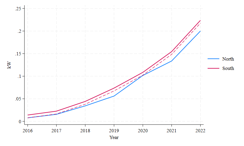
Figure 18: DiD - Border 2, 2016-2022 (kW)

A visual inspection of figures 18 and 19 indicates that the divergence in installed PV capacity is less pronounced when municipalities in greater geographical distance from the tariff border are considered. In this case there is especially no divergence in installed PV per capita levels before 2020.

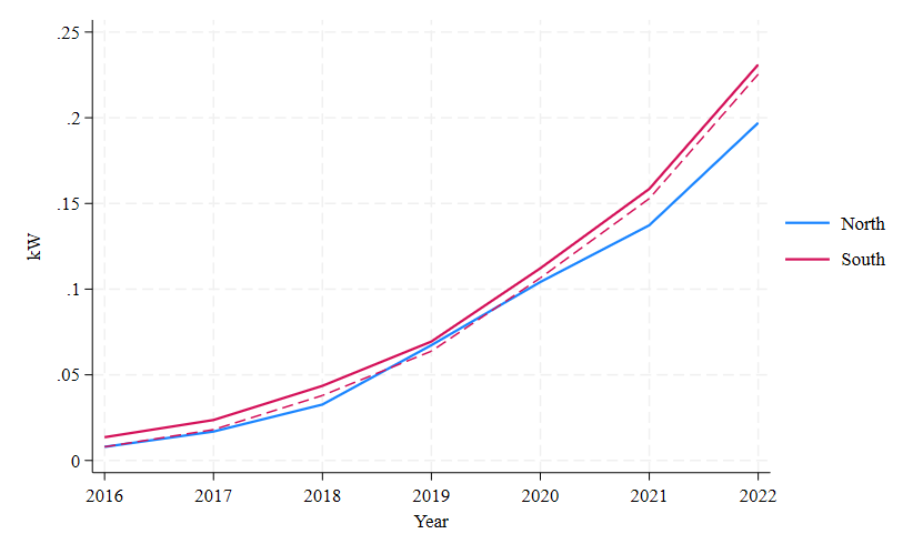
Figure 19: DiD - Border 3, 2016-2022 (kW)

To test whether the underlying assumptions are violated, a parallel trends and a placebo test are conducted. For the placebo test it is assumed that treatment already occurs in 2018, hence 2 year before the actual treatment

Table 8: Parallel trends assumption

	Border 1	Border 2	Border 3
North	0.000	0.000	0.000
	(.)	(.)	(.)
South	-7.483	-7.480	1.293
	(0.30)	(0.36)	(0.89)
Year	0.011***	0.016***	0.019***
	(0.00)	(0.00)	(0.00)
North x Year	0.000	0.000	0.000
	(.)	(.)	(.)
South x Year	0.004	0.004	-0.001
	(0.30)	(0.36)	(0.90)
Constant	-22.203***	-32.942***	-39.067***
	(0.00)	(0.00)	(0.00)
Robust standard errors in parentheses
*** p$<$0.01, ** p$<$0.05, * p$<$0.1

According to the results in table 8, the assumption of parallel pre-treatment trends holds for all border definition. This is indicated by the insignificance of the interaction term between the time variable Year and membership in the control group South.

Table 9: Placebo test

	Border 1		Border 2		Border 3
	(1)	(2)	(3)	(4)	(5)	(6)
ATET	-0.019***	-0.007	-0.009***	-0.002	-0.009***	0.019***
	(0.000)	(.)	(0.000)	(.)	(0.000)	(0.000)
Income		-0.000		-0.000		-0.000***
		(.)		(.)		(0.001)
Housing		1.417		-1.320		1.301**
		(.)		(.)		(0.006)
Unemployment		-0.005		-0.006		0.012***
		(.)		(.)		(0.001)
Constant	0.009*	0.880	0.011*	1.420	0.011*	2.258**
	(0.042)	(.)	(0.017)	(.)	(0.024)	(0.001)
Year FE	Yes	Yes	Yes	Yes	Yes	Yes
Robust standard errors in parentheses
*** p$<$0.01, ** p$<$0.05, * p$<$0.1

Unlike the parallel pre-treatment trends, the placebo test results in table 9, displays significant estimates for both specifications of border 3 and for border 1 and 2 are included. This suggests, that something else than tariff-divergence in 2020 is driving difference in PV uptake across BZ.

References

- Abadie (2021) Abadie, A. (2021). Using synthetic controls: Feasibility, data requirements, and methodological aspects. Journal of Economic Literature 59(2), 391–425.
- Abadie et al. (2010) Abadie, A., A. Diamond, and J. Hainmueller (2010). Synthetic control methods for comparative case studies: Estimating the effect of california’s tobacco control program. Journal of the American statistical Association 105(490), 493–505.
- Abadie et al. (2015) Abadie, A., A. Diamond, and J. Hainmueller (2015). Comparative politics and the synthetic control method. American Journal of Political Science 59(2), 495–510.
- Abadie and Gardeazabal (2003) Abadie, A. and J. Gardeazabal (2003). The economic costs of conflict: A case study of the basque country. American economic review 93(1), 113–132.
- Andersson et al. (2021) Andersson, J., H. Hellsmark, and B. Sandén (2021). Photovoltaics in sweden–success or failure? Renewable and Sustainable Energy Reviews 143, 110894.
- Angrist and Pischke (2009) Angrist, J. D. and J.-S. Pischke (2009). Mostly harmless econometrics: An empiricist’s companion. Princeton university press.
- Armelius (2012) Armelius, H. (2012). Elbrist. Available at energifakta.se.
- Assunção and Schutze (2017) Assunção, J. and A. Schutze (2017). Developing brazil’s market for distributed solar generation. Climate Policy Initiative Police Brief 1(17518695), 2020.
- Baginski and Weber (2019) Baginski, J. P. and C. Weber (2019). Coherent estimations for residential photovoltaic uptake in germany including spatial spillover effects.
- Balta-Ozkan et al. (2015) Balta-Ozkan, N., J. Yildirim, and P. M. Connor (2015). Regional distribution of photovoltaic deployment in the uk and its determinants: A spatial econometric approach. Energy Economics 51, 417–429.
- Berg (2023) Berg, M. (2023). Därför tar tillstånden för vindkraft längre tid i sverige. Available at energi.se.
- Bergek (2010) Bergek, A. (2010). Levelling the playing field? the influence of national wind power planning instruments on conflicts of interests in a swedish county. Energy policy 38(5), 2357–2369.
- Bergek and Jacobsson (2010) Bergek, A. and S. Jacobsson (2010). Are tradable green certificates a cost-efficient policy driving technical change or a rent-generating machine? lessons from sweden 2003–2008. Energy policy 38(3), 1255–1271.
- Billmeier and Nannicini (2013) Billmeier, A. and T. Nannicini (2013). Assessing economic liberalization episodes: A synthetic control approach. Review of Economics and Statistics 95(3), 983–1001.
- Blom Westergren (2022) Blom Westergren, E. (2022). Lång väntetid och många konflikter kring solceller. Available at byggahus.se.
- Bloomberg (2022) Bloomberg (2022). Solar panels piling up in warehouses in energy-starved europe. Available at bloomberg.com.
- Borenstein (2017) Borenstein, S. (2017). Private net benefits of residential solar pv: The role of electricity tariffs, tax incentives, and rebates. Journal of the Association of Environmental and Resource Economists 4(S1), S85–S122.
- Breuer and Moser (2014) Breuer, C. and A. Moser (2014). Optimized bidding area delimitations and their impact on electricity markets and congestion management. In 11th International Conference on the European Energy Market (EEM14), pp. 1–5. IEEE.
- Briguglio and Formosa (2017) Briguglio, M. and G. Formosa (2017). When households go solar: Determinants of uptake of a photovoltaic scheme and policy insights. Energy Policy 108, 154–162.
- Card (1990) Card, D. (1990). The impact of the mariel boatlift on the miami labor market. ILR Review 43(2), 245–257.
- Castillo et al. (2016) Castillo, C. P., F. B. e Silva, and C. Lavalle (2016). An assessment of the regional potential for solar power generation in eu-28. Energy policy 88, 86–99.
- da Silva et al. (2016) da Silva, R. C., I. de Marchi Neto, and S. S. Seifert (2016). Electricity supply security and the future role of renewable energy sources in brazil. Renewable and Sustainable Energy Reviews 59, 328–341.
- Dagens industri (2023) Dagens industri (2023). Om tyskland inför elprisområden sänker vi elpriserna i södra sverige. Available at di.se.
- dos Santos Carstens and da Cunha (2019) dos Santos Carstens, D. D. and S. K. da Cunha (2019). Challenges and opportunities for the growth of solar photovoltaic energy in brazil. Energy policy 125, 396–404.
- Dube and Zipperer (2015) Dube, A. and B. Zipperer (2015). Pooling multiple case studies using synthetic controls: An application to minimum wage policies. Available at SSRN 2589786.
- ECEEE (2023) ECEEE (2023). The european green deal. Available at eceee.org.
- Energimyndigheten (2013) Energimyndigheten (2013). Solelprogrammet fram till 2018. Available at energiforsk.se.
- Energimyndigheten (2020) Energimyndigheten (2020). National survey report of pv power applications in sweden. Available at iea-pvps.org.
- Energimyndigheten (2023a) Energimyndigheten (2023a). Nätanslutna solcellsanläggningar. Available at energimyndigheten.se.
- Energimyndigheten (2023b) Energimyndigheten (2023b). Solelportalen. Available at energimyndigheten.se.
- ENTSO-E (2023) ENTSO-E (2023). Bidding zone review. Available at entsoe.eu.
- EU (2020) EU (2020). State of the union 2020. Available at europa.eu.
- Fischer and Strauss (2021) Fischer, G. and R. Strauss (2021). Europe’s Income, Wealth, Consumption, and Inequality. International Policy Exchange.
- Fridolfsson and Tangerås (2013) Fridolfsson, S.-O. and T. P. Tangerås (2013). A reexamination of renewable electricity policy in sweden. Energy Policy 58, 57–63.
- Gautier and Jacqmin (2020) Gautier, A. and J. Jacqmin (2020). Pv adoption: the role of distribution tariffs under net metering. Journal of Regulatory Economics 57(1), 53–73.
- Graziano and Gillingham (2015) Graziano, M. and K. Gillingham (2015). Spatial patterns of solar photovoltaic system adoption: the influence of neighbors and the built environment. Journal of Economic Geography 15(4), 815–839.
- Hancock (2023) Hancock, A. (2023). Europe’s solar industry warns of bankruptcies over chinese imports. Available at ft.com.
- Hogan et al. (2022) Hogan, J. L., C. R. Warren, M. Simpson, and D. McCauley (2022). What makes local energy projects acceptable? probing the connection between ownership structures and community acceptance. Energy Policy 171, 113257.
- Hurta et al. (2022) Hurta, A., M. Žilka, and F. Freiberg (2022). Impact of the splitting of the german–austrian electricity bidding zone on investment in a grid-scale battery energy storage system deployed for price arbitrage with gray and green power in austrian and german day-ahead power markets. Energy Reports 8, 12045–12062.
- IEA (2019) IEA (2019). Finland tender-based feed-in premium scheme for renewable power generation (30.12.2010/1396). Available at iea.org.
- IEA (2022) IEA (2022). Trends in pv applications 2022. Available at iea-pvps.org.
- IEA (2023) IEA (2023). Sweden. Available at iea.org.
- IRENA (2021) IRENA (2021). Renewable power generation costs in 2020. Available at irena.org.
- Janda et al. (2017) Janda, K., J. Málek, and L. Rečka (2017). Influence of renewable energy sources on transmission networks in central europe. Energy Policy 108, 524–537.
- Johnson (2021) Johnson, S. (2021). Pulling power: the green lure of sweden’s industrial far north. Available at arctictoday.com.
- Katanich (2023) Katanich, D. (2023). Clean energy or crops? solar panel projects divide families in the us. Available at euronews.com.
- Keisha (2022) Keisha, F. (2022). Difference-in-differences. Available at medium.com.
- Kurmayer (2023) Kurmayer, N. J. (2023). Germany gears up for eu fight over electricity bidding zones. Available at euractiv.com.
- Lee and Ebong (2017) Lee, T. D. and A. U. Ebong (2017). A review of thin film solar cell technologies and challenges. Renewable and Sustainable Energy Reviews 70, 1286–1297.
- Mauritzen (2023) Mauritzen, J. (2023). With great power (prices) comes great tail pipe emissions?a natural experiment of electricity prices and electric car adoption. arXiv preprint arXiv:2304.01709.
- McManus (2012) McManus, M. C. (2012). Environmental consequences of the use of batteries in low carbon systems: The impact of battery production. Applied Energy 93, 288–295.
- Miljödepartementet (2019) Miljödepartementet (2019). Sweden’s draft integrated national energy and climate plan. Available at government.se.
- Miljödepartementet (2020) Miljödepartementet (2020). Sweden’s long-term strategy for reducing greenhouse gas emissions. Available at unfccc.int.
- Ofgem (2014) Ofgem, F. T. (2014). Bidding zones literature review.
- Öhrlund et al. (2020) Öhrlund, I., B. Stikvoort, M. Schultzberg, and C. Bartusch (2020). Rising with the sun? encouraging solar electricity self-consumption among apartment owners in sweden. Energy Research & Social Science 64, 101424.
- Oliveira (2023) Oliveira, T. (2023). Bidding zones. Available at synertics.io.
- Our World in data (2023a) Our World in data (2023a). Installed solar energy capacity. Available at ourworldindata.org.
- Our World in data (2023b) Our World in data (2023b). Share of electricity production from renewables. Available at ourworldindata.org.
- Our World in data (2023c) Our World in data (2023c). Share of electricity production from solar. Available at ourworldindata.org.
- Palm (2020) Palm, A. (2020). Early adopters and their motives: Differences between earlier and later adopters of residential solar photovoltaics. Renewable and Sustainable Energy Reviews 133, 110142.
- Panwar et al. (2011) Panwar, N., S. Kaushik, and S. Kothari (2011). Role of renewable energy sources in environmental protection: A review. Renewable and sustainable energy reviews 15(3), 1513–1524.
- PV Magazine (2022) PV Magazine (2022). Feed-in tariffs (fits) in europe. Available at pv-magazine.com.
- Regeringskansliet (2015) Regeringskansliet (2015). The swedish innovation strategy. Available at government.se.
- Richardson and Troost (2009) Richardson, G. and W. Troost (2009). Monetary intervention mitigated banking panics during the great depression: quasi-experimental evidence from a federal reserve district border, 1929–1933. Journal of Political Economy 117(6), 1031–1073.
- Satpute et al. (2020) Satpute, S. D., J. S. Jagtap, P. K. Bhujbal, S. M. Sonar, P. K. Baviskar, H. M. Pathan, et al. (2020). Mercurochrome sensitized zno/in2o3 photoanode for dye-sensitized solar cell. ES Energy & Environment 9(5), 89–94.
- SCB (2022) SCB (2022). Statistics sweden. Available at scb.se.
- Schmidt et al. (2016) Schmidt, J., R. Cancella, and A. O. Pereira Jr (2016). An optimal mix of solar pv, wind and hydro power for a low-carbon electricity supply in brazil. Renewable Energy 85, 137–147.
- Sena et al. (2016) Sena, L. A. d., P. Ferreira, and A. C. Braga (2016). Social acceptance of wind and solar power in the brazilian electricity system. Environment, development and sustainability 18, 1457–1476.
- SHE (2022) SHE (2022). Elomraaden. Available at sheab.se.
- Smart City Sweden (2023) Smart City Sweden (2023). The green industrial revolution happens in northern sweden. Available at smartcitysweden.com.
- SMHI (2022) SMHI (2022). Strålning. Available at smhi.se.
- SMHI (2023) SMHI (2023). StrÅng - a mesoscale model for solar radiation. Available at strang.smhi.se.
- Stede and May (2019) Stede, J. and N. May (2019). Strikte mindestabstände bremsen den ausbau der windenergie. DIW Wochenbericht 86(48), 895–903.
- Strom-Report (2021) Strom-Report (2021). Electricity prices in europe – who pays the most? Available at strom-report.com.
- Svenska Kraftnät (2022) Svenska Kraftnät (2022). Nätområden.se. Available at natomraden.se.
- Swedish Energy Markets Inspectorate (2022) Swedish Energy Markets Inspectorate (2022). Elområde. Available at ei.se.
- Swedish Government (2020) Swedish Government (2020). Sweden’s integrated national energy and climate plan. Available at energy.ec.europa.eu.
- Tagesschau (2022) Tagesschau (2022). Nordländer fordern strompreiszonen. Available at tagesschau.de.
- Tamimi et al. (2013) Tamimi, B., C. Cañizares, and K. Bhattacharya (2013). System stability impact of large-scale and distributed solar photovoltaic generation: The case of ontario, canada. IEEE transactions on sustainable energy 4(3), 680–688.
- Thunborg (2021) Thunborg, P. (2021). Elpriset tynger företag i södra sverige. Available at foretagarna.se.
- Tidöavtalet (2022) Tidöavtalet (2022). Överenskommelse för sverige. Available at moderaterna.se.
- Van den Bergh et al. (2016) Van den Bergh, K., C. Wijsen, E. Delarue, and W. D’haeseleer (2016). The impact of bidding zone configurations on electricity market outcomes. In 2016 IEEE International Energy Conference (ENERGYCON), pp. 1–6. IEEE.
- Vattenfall (2023) Vattenfall (2023). Prishistorik över rörliga elpriser. Available at vattenfall.se.
- Winter and Schlesewsky (2019) Winter, S. and L. Schlesewsky (2019). The german feed-in tariff revisited-an empirical investigation on its distributional effects. Energy Policy 132, 344–356.
- Yang et al. (2020) Yang, Y., P. E. Campana, B. Stridh, and J. Yan (2020). Potential analysis of roof-mounted solar photovoltaics in sweden. Applied Energy 279, 115786.
- Zeldow and Hatfield (2023) Zeldow, B. and L. Hatfield (2023). Difference-in-differences. Available at healthpolicydatascience.org.
- Zhang et al. (2011) Zhang, Y., J. Song, and S. Hamori (2011). Impact of subsidy policies on diffusion of photovoltaic power generation. Energy Policy 39(4), 1958–1964.
- Zinke (2021) Zinke, O. (2021). Solarparks auf fruchtbaren Äckern – flächenfraß für die umwelt? Available at agrarheute.com.