SymmPI: Predictive Inference for Data
with Group Symmetries

Abstract

Quantifying the uncertainty of predictions is a core problem in modern statistics. Methods for predictive inference have been developed under a variety of assumptions, often—for instance, in standard conformal prediction—relying on the invariance of the distribution of the data under special groups of transformations such as permutation groups. Moreover, many existing methods for predictive inference aim to predict unobserved outcomes in sequences of feature-outcome observations. Meanwhile, there is interest in predictive inference under more general observation models (e.g., for partially observed features) and for data satisfying more general distributional symmetries (e.g., rotationally invariant or coordinate-independent observations in physics). Here we propose SymmPI, a methodology for predictive inference when data distributions have general group symmetries in arbitrary observation models. Our methods leverage the novel notion of distributional equivariant transformations, which process the data while preserving their distributional invariances. We show that SymmPI has valid coverage under distributional invariance and characterize its performance under distribution shift, recovering recent results as special cases. We apply SymmPI to predict unobserved values associated to vertices in a network, where the distribution is unchanged under relabelings that keep the network structure unchanged. In several simulations in a two-layer hierarchical model, and in an empirical data analysis example, SymmPI performs favorably compared to existing methods.

1 Introduction

Prediction is one of the most important problems in modern statistical learning. Since unobserved data cannot always be predicted with certainty, quantifying the uncertainty of predictions is a crucial statistical problem, studied in the areas of predictive inference and conformal prediction (e.g., Geisser, 2017; Vovk et al., 2005). Numerous predictive inference methods have been developed under both parametric and nonparametric conditions (e.g., Wilks, 1941; Wald, 1943; Vovk et al., 1999, 2005; Lei et al., 2013; Lei, 2014; Chernozhukov et al., 2018; Romano et al., 2019, etc); see the related work section for more examples.

Among these, conformal prediction (or inference) has been gaining increasing attention recently because it can lead to prediction sets with finite-sample coverage guarantees under reasonable conditions on the data, such as the exchangeability of the datapoints. Moreover, this exchangeability condition is preserved under natural permutation-equivariant maps (see e.g., Dean and Verducci, 1990; Kuchibhotla, 2020). This implies that residuals constructed from statistical learning methods that are invariant with respect to the data—such as $M$-estimators—remain exchangeable, and can be used for conformal inference. Conformal prediction has been applied and extended to a wide range of statistical machine learning problems, including non-parametric density estimation and regression (Lei et al., 2013; Lei and Wasserman, 2014; Lei et al., 2018), quantile regression (Romano et al., 2019), survival analysis (Candès et al., 2023; Gui et al., 2022), etc.

At the same time, predictive inference methods have been developed under assumptions different from exchangeable independent and identically distributed data, including for datapoints $Z_{n}$ in sequential observation models called online compression models leading to data $Z_{1},\ldots,Z_{n-1}\in\mathcal{Z}_{0}$ for some space $\mathcal{Z}_{0}$, and for non-sequential models called one-off-structures (Vovk et al., 2005). These are closely related to the classical statistical notion of conditional ancillarity (Cox, 2006; Dobriban and Lin, 2023). Methods have also been developed under more concrete assumptions such as hierarchical exchangeability (Lee et al., 2023), exchangeable network data (Lunde et al., 2023), and invariance under a finite subgroup of the permutations of the datapoints (Chernozhukov et al., 2018).

However, at the moment there are no predictive inference methods (1) for arbitrary unobserved functions of arbitrary data $Z$ (e.g., a network, a function, etc.) whose distributional symmetries are characterized by an arbitrary—possibly infinite and continuous—group (e.g., a rotation group that arises for coordinate-independent data); and (2) that enable processing the data in flexible ways to keep the distributional symmetries, similar to what is possible in the special case of conformal prediction. In this paper, we develop such methods. More specifically:

• We consider datasets whose distributions are invariant under general—compact Hausdorff topological—groups. We argue that invariance under such groups is of broad interest, and includes in particular invariance under all finite groups (e.g., exchangeability, hierarchical exchangeability, cyclic shifts). It also includes invariance under continuous groups such as rotations (and combinations such as rotations and translations), which are of broad interest in the physical sciences. For example many quantities are coordinate-independent and thus rotation-invariant in physics (Gross, 1996; Robinson, 2011; Schwichtenberg, 2018). Continuous (e.g., rotational) invariances are also common for image data. The datasets we consider are not restricted in any other way, and in particular we are not limited to sequential observations $Z_{1},\ldots,Z_{n}$.

• We introduce the key notion of distributional equivariance of transformations of the data, and show that it is enough to preserve distributional invariance. We explain how this allows us to process data to extract meaningful features that enables constructing accurate prediction sets, and—for instance—adapting to data heterogeneity in a two-layer hierarchical model example. We also allow arbitrary group actions on the input and output spaces, not limited e.g., to permutation actions. We allow the observed component of the data be determined by an arbitrary function that we call the observation function. For instance, this can include any part of the features in a supervised learning setting. In particular, we are not limited to predicting an outcome $Y_{n}$ after observing feature-label pairs $(X_{1},Y_{1}),\ldots,(X_{n-1},Y_{n-1})$, and a feature $X_{n}$.

• We propose SymmPI, a method for predictive inference for data with distributional symmetries in the above setting. We show that SymmPI has coverage greater than or equal to the nominal level, and not much more than that, under distributional invariance. We bound the over-coverage in terms of a group-theoretical quantity (the number of orbits of the action of the group). We further bound the impact of distribution shift, i.e., the lack of distributional invariance, on the coverage. Finally, we introduce a non-symmetric version of SymmPI for the distribution shift case where the processing algorithm is not distributionally equivariant, and provide associated coverage guarantees. In the special case of conformal prediction, we recover recent results of Barber et al. (2023).

• As an illustration of SymmPI, we study the example of prediction sets on networks, where random variables associated with a network are assumed to have a distribution invariant under any transformation that keeps the network structure unchanged (i.e., to the automorphism group of the graph). We study in detail the example of hierarchical two-layer models with several sub-populations (Dunn et al., 2022; Sesia et al., 2023) (also known as meta-learning with several tasks (Park et al., 2022)). We design a data processing architecture based on a fixed message-passing graph neural network. We show that SymmPI with this architecture adapts to heterogeneity over sub-populations or tasks, and performs favorably compared to prior methods, including standard conformal prediction and the algorithm from Dunn et al. (2022).

Our paper is structured as follows: In Section 2, we introduce preliminaries from group theory used in our work, and notions of distributional equivariance and invariance. In Section 3, we provide a detailed review of previous research relevant to our study. In Section 4, we introduce our novel approach, referred to as SymmPI, and discuss its underlying theoretical principles and guarantees. Additionally, in Section 5, we illustrate the practical application of SymmPI through a two-layer hierarchical model and substantiate its effectiveness through numerical experiments. A software implementation of the methods used in this paper, along with the code necessary to reproduce our numerical results, is available at https://github.com/MaxineYu/Codes_SymmPI.

Notation. For a positive integer $m\geqslant 1$, the $m$-dimensional all-ones vector is denoted as $1_{m}=(1,1,\ldots,1)^{\top}\in\mathbb{R}^{m}$ and the all-zeros vector is $0_{m}=(0,\ldots,0)^{\top}\in\mathbb{R}^{m}$. We denote $[m]:=\{1,2,\ldots,m\}$, and for $j\in[m]$, the $j$-th standard basis vector by $e_{j}=(0,\ldots,1,\ldots,0)^{\top}$, where only the $j$-th entry equals unity, and all other entries equal zero. For two random objects $X,Y$, we denote by $X=_{d}Y$ that they have the same distribution. For a probability distribution $\Gamma$ and a random variable $X\sim\Gamma$, we may write the probability that $X$ belongs to a measurable set $A$ as $P(X\in A)$, $P_{X}(A)$, $P_{\Gamma}(X\in A)$, $P_{X\sim\Gamma}(X\in A)$, $\Gamma(X\in A)$, or $\Gamma(A)$. For a cumulative distribution function (c.d.f.) $F$ on $\mathbb{R}$, and $\alpha\in[0,1]$, the $1-\alpha$-th population quantile is $q_{1-\alpha}(F)=F^{-1}({1-\alpha})=\inf\{x:F(x)\geqslant{1-\alpha}\}$, with $q_{1-\alpha}(F)=\infty$ if the set is empty. The $1-\alpha$-quantile of the random variable $X$, for $\alpha\in[0,1]$, is $Q_{1-\alpha}(X)$. For $c\in\mathbb{R}^{k}$, let $\delta_{c}$ be the point mass at $c$. For a vector $v\in\mathbb{R}^{m}$, $Q_{1-\alpha}(v)=Q_{1-\alpha}(v_{1},\ldots,v_{m})$ denotes $Q_{1-\alpha}(\sum_{i=1}^{m}\delta_{v_{i}}/m)$.

2 Preliminaries

We introduce our predictive inference method based on the notions of distributional equivariance and invariance.

2.1 Review of Group Theoretic Background

First we provide a self-contained review of some basic material from group theory that is required in our work. We refer to e.g., Giri (1996); Diaconis (1988); Nachbin (1976); Folland (2016); Diestel and Spalsbury (2014); Tornier (2020) for additional details. Readers may skip ahead to Section 2.2 and refer back to this section as needed.

A group $\mathcal{G}$ is a set endowed with a binary operation “$\cdot$” which is associative, in the sense that for all $g,g^{\prime},g^{\prime\prime}\in\mathcal{G}$, $(g\cdot g^{\prime})\cdot g^{\prime\prime}=g\cdot(g^{\prime}\cdot g^{\prime\prime})$. Further, a group has an identity element (or unit, or neutral element) denoted as $1_{\mathcal{G}}$ or $e_{\mathcal{G}}$, such that for all $g\in\mathcal{G}$, $e_{\mathcal{G}}g=ge_{\mathcal{G}}=g$. The subscript of the identity is dropped if no confusion can arise. Finally, each group element $g$ has an inverse $g^{-1}$ such that $g\cdot g^{-1}=1_{\mathcal{G}}$.

A key example is the symmetric group $\mathrm{S}_{n}$ of permutations of $n\geqslant 1$ elements $\mathrm{S}_{n}=\{\pi:[n]\to[n]\mid\pi\,\mathrm{permutation}\}$, where the multiplication $\pi\cdot\pi^{\prime}$ corresponds to the composition $\pi\circ\pi^{\prime}$ of the permutations. Moreover the identity element $1_{\mathcal{G}}$ is the identity map with $1_{\mathcal{G}}(x)=x$ for all $x\in[n]$, and the group inverse of any permutation $\pi$ is its functional inverse $\pi^{-1}$. Other important groups are the group $\mathrm{O}(n)$ of orthogonal rotations and reflections of $\mathbb{R}^{n}$ and the special orthogonal group $\mathrm{SO}(n)$ of rotations of $\mathbb{R}^{n}$.

For a group $\mathcal{G}$, the map $\rho:\mathcal{G}\times\mathcal{Z}\to\mathcal{Z}$ is an action of $\mathcal{G}$ on $\mathcal{Z}$, if for all $g,g^{\prime}\in\mathcal{G}$ and $z\in\mathcal{Z}$, $\rho(gg^{\prime},z)=\rho(g,\rho(g^{\prime},z))$; and if for all $z\in\mathcal{Z}$, $\rho(e,z)=z$. We denote $\rho(g,z):=\rho(g)z$ for both non-linear and linear actions $\rho$. This notation takes special meaning when $\rho$ acts linearly, in which case $\rho$ is called a representation and we think of $\rho(g):\mathcal{Z}\to\mathcal{Z}$ as a linear map.

Example 2.1 (Permutation action).

For any space $\mathcal{Z}_{0}$, the symmetric group $\mathrm{S}_{n}$ acts on $\mathcal{Z}_{0}^{n}$ by the permutation action $\rho$, which permutes the coordinates of the input, such that for all $g\in\mathrm{S}_{n}$ and $z\in\mathcal{Z}_{0}^{n}$, $g\cdot x:=\rho(g)x:=(z_{g^{-1}(1)},\ldots,z_{g^{-1}(n)})^{\top}$.

For a general group, the orbit of $z$ under $\rho$ is the set $O_{z}=\{\rho(g)z,g\in\mathcal{G}\}$, and includes the subset of $\mathcal{Z}$ that can be reached by the action of $\mathcal{G}$ on $z$. For instance the orbit of $(1,2)^{\top}$ under $\mathrm{S}_{2}$ is $\{(1,2)^{\top},(2,1)^{\top}\}$, while that of $(1,1)^{\top}$ is $\{(1,1)^{\top}\}$.

Certain groups are also topological spaces (Munkres, 2019), with associated open sets. In that case, one can construct the Borel sigma algebra generated by the open sets. For certain groups—Specifically, for compact Hausdorff topological groups—there is a “uniform” (Haar) probability measure $U$ over the group endowed with the Borel sigma algebra (see e.g., Diestel and Spalsbury, 2014). For a finite group such as $\mathrm{S}_{n}$, this is the discrete uniform measure. In general, the Haar probability measure satisfies that for any $g\in\mathcal{G}$, and $G\sim U$, we have $gG\sim U$. We will only consider groups that have a Haar probability measure.

2.2 Distributional Equivariance and Invariance

We consider a dataset $Z$, belonging to a measurable space $\mathcal{Z}$, such as an Euclidean space. This will also be referred to as the complete dataset, because we observe only part of $Z$; as explained later in Section 4.1. This dataset is completely general: as special cases, it can represent labeled observations in a supervised learning setting, i.e., $Z=((X_{1},Y_{1}),\ldots,(X_{n},Y_{n}))^{\top}$, or unlabeled observations in unsupervised learning, i.e., $Z=(X_{1}\ldots,X_{n})^{\top}$.

The complete data $Z$ has an unknown distribution $P$ belonging to a set $\mathcal{P}$ of probability distributions. Consider a measurable map $f:\mathcal{Z}\to\tilde{\mathcal{Z}}$ for some measurable space $\tilde{\mathcal{Z}}$, which we can think of as a transformation of the data. This transformation can either be designed by hand, or learned in appropriate ways. For instance, in a supervised learning setting where $Z=((X_{1},Y_{1}),\ldots,(X_{n},Y_{n}))^{\top}\in(\mathcal{X}\times\mathcal{Y})^{n}$, and for a predictor $\hat{\mu}:\mathcal{X}\to\mathcal{Y}$ learned based on $Z$, we may have $f(Z)=(|Y_{1}-\hat{\mu}(X_{1})|,\ldots,|Y_{n}-\hat{\mu}(X_{n})|)^{\top}$. Further examples and discussion will be provided in our illustrations in Section 5.

We consider a known group $\mathcal{G}$ that acts on the complete data space $\mathcal{Z}$ by the action $\rho$ of $\mathcal{G}$, and on the transformed data space $\tilde{\mathcal{Z}}$ by the action $\tilde{\rho}$ of $\mathcal{G}$. When $Z=((X_{1},Y_{1}),\ldots,(X_{n},Y_{n}))^{\top}$, these can be the standard permutation action of the symmetric group $\mathrm{S}_{n}$ from Example 2.1, such that $\rho(g)Z=((X_{g^{-1}(1)},Y_{g^{-1}(1)}),\ldots,(X_{g^{-1}(n)},Y_{g^{-1}(n)}))^{\top}$, and $\rho(g)f(Z)=(|Y_{g^{-1}(1)}-\hat{\mu}(X_{g^{-1}(1)})|,\ldots,|Y_{g^{-1}(n)}-\hat{\mu}(X_{g^{-1}(n)})|)^{\top}$.

A key property of the map $f$ that we will use to construct prediction regions is that $f$ respects the symmetry of the group, in a distributional sense. This is formalized in our definition of distributional equivariance given below. For two random objects $X,Y$, recall that we denote by $X=_{d}Y$ that they have the same distribution.

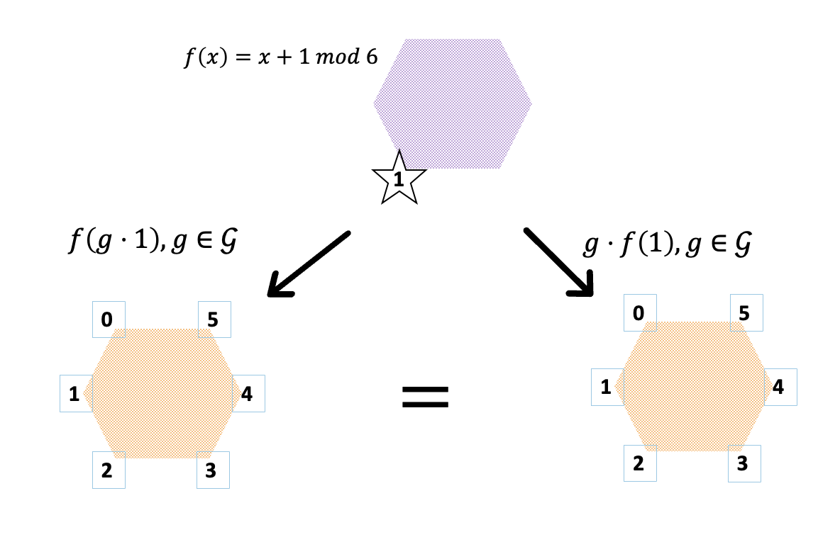
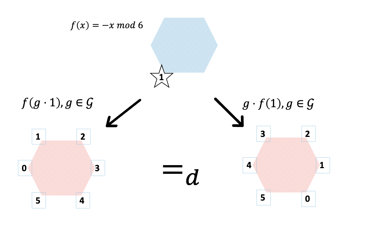
Figure 1: Illustration of determistically and distributionally equivariant maps. We consider the domain $\mathcal{Z}=\{0,1,2,3,4,5\}$ with a uniform measure and the group $\mathcal{G}=(\mathbb{Z}_{6},+)=(\{0,1,2,3,4,5\},+)$, where the group operation $g\cdot z,z\in\mathcal{Z}$ is defined as $g+z$ modulo $6$. In the left panel, we present a deterministically equivariant map defined by $f(z)=z+1$ modulo $6$ for all $z\in\mathcal{Z}$, with $f(g+z)=g+f(z)$ modulo $6$ for all $z\in\mathcal{Z},g\in\mathcal{G}$; and note that all deterministically equivariant maps are of the form $x\mapsto x+a$ modulo $6$ for some $a\in\mathcal{Z}$. In contrast, all maps are distributionally equivariant. As an illustration, in the right panel, we show the distributionally (but not deterministically) equivariant map $x\mapsto-x$ modulo $6$.

Definition 2.2 (Distributional equivariance).

We say that the map $f:\mathcal{Z}\to\tilde{\mathcal{Z}}$ is $\mathcal{G}$-distributionally equivariant (with respect to the actions $\rho,\tilde{\rho}$ on $\mathcal{Z},\tilde{\mathcal{Z}}$ respectively, and over the class $\mathcal{P}$ of probabilities), when for all $P\in\mathcal{P}$, for $Z\sim P$ and for an independently drawn group element $G\sim U$ from the uniform probability distribution $U$ over $\mathcal{G}$, we have the equality in distribution

$$f(\rho(G)Z)=_{d}\tilde{\rho}(G)f(Z).$$ (1)

This means that the distribution of a randomly chosen action of $\mathcal{G}$ on $Z$, transformed by $f$, is equal to the distribution found by first transforming $Z$ by $f$, and then randomly acting on it by $\mathcal{G}$. In a distributional sense, the random action of $\mathcal{G}$ and the deterministic transform $f$ “commute”. This definition generalizes the classical notion of deterministic $\mathcal{G}$-equivariance, which requires that for all $z\in\mathcal{Z}$ and all $g\in\mathcal{G}$,

$$f(\rho(g)z)=\tilde{\rho}(g)f(z).$$ (2)

Deterministic equivariance is widely studied in the mathematical area of representation theory (e.g., Fulton and Harris, 2013). Distributional equivariance only requires the equality of the distributions of $f(\rho(G)Z)$ and $\tilde{\rho}(G)f(Z)$ for random $Z,G$, whereas deterministic equivariance requires (2) to hold for for all $z\in\mathcal{Z}$ and all $g\in\mathcal{G}$. Deterministic equivariance clearly implies the distributional version. We characterize these conditions in Section 7.1, showing that distributional equivariance is a strictly more general condition than the deterministic version. Moreover, in Figure 1, we use a toy example to illustrate the difference between distributionally and deterministically equivariant maps. For some positive integer $M$, we consider the action of the group of cyclic shifts $z\mapsto z+a$ modulo $M$ on itself. We show in Section 7.1 that deterministic equivariance requires affine maps $z\mapsto z+a$ modulo $M$, for any $a$, while distributional equivariance is satisfied by all maps.

A key example of distributional equivariance is distributional invariance, namely $f(\rho(G)Z)$ $=_{d}$ $f(Z)$. This condition states that after applying the map $f$, the distributions of the original data $Z$ and the data $\rho(G)Z$ acted upon by the group are equal. This is a special case of Definition 2.2 for an identity output representation $\tilde{\rho}(g)=1$ for all $g\in\mathcal{G}$. For the identity map $f$, taking any $g^{\prime}\in\mathcal{G}$, we can deduce from it that $\rho(g^{\prime})Z=_{d}\rho(g^{\prime})\rho(G)Z=_{d}\rho(G)Z=_{d}Z$. Hence for the identity map $f$, distributional equivariance implies that $Z=_{d}\rho(g^{\prime})Z$ for all $g^{\prime}\in\mathcal{G}$. This latter condition has been widely studied; for instance in analyzing randomization tests (Dobriban, 2022) and data augmentation (Chen et al., 2020; Chatzipantazis et al., 2023). We analyze this condition further in Section 7.1.3.

Consider a fixed $z\in\mathcal{Z}$ and let $O_{z}=\{\rho(g)z:g\in\mathcal{G}\}$ be the orbit of $z$ under $\mathcal{G}$. The distribution of $\rho(G)z$ when $G\sim U$ can be viewed as a uniform distribution over the orbit $O_{z}$ with the sigma-algebra generated by the intersection of $O_{z}$ with the sigma-algebra over $\mathcal{Z}$. Since this distribution is the same regardless of the distribution $P$ of $Z$, the data $Z$ is conditionally ancillary given the orbits, see also Chen et al. (2020); Dobriban and Lin (2023). This shows that distributional invariance as in $\rho(G)Z$ $=_{d}$ $Z$ is a form of conditional ancillarity. Conditional ancillarity is one of the most general conditions under which finite-sample valid predictive inference methods have been designed (see Section 3).

2.2.1 Examples

We give a few examples of distributional equivariance and invariance. Since we will later consider only part of $Z$ as observed, we will here let $Z$ contain $n+1$ observations, where the $(n+1)$st will later not be fully observed.

1. Exchangeable data. Take $\mathcal{Z}=\mathcal{Z}_{0}^{n+1}$, for some space $\mathcal{Z}_{0}$, and the group $\mathcal{G}$ as the permutation group $\mathrm{S}_{n+1}$, acting on $\mathcal{Z}$ by permuting the coordinates as $\rho(g)Z:=gZ=$ $(Z_{g^{-1}(1)},$ $\ldots,Z_{g^{-1}(n+1)})^{\top}$ for $Z=(Z_{1},\ldots,Z_{n+1})^{\top}$. Then for the identity map $f:\mathcal{Z}\to\mathcal{Z}$, with $f(z)=z$ for all $z\in\mathcal{Z}$, the distributional invariance condition reduces to the vector $Z$ having exchangeable components.

2. Network-structured data. We take the data $Z=(Z_{1},\ldots,Z_{n+1})^{\top}\in\mathcal{Z}_{0}^{n+1}$ as before, but we only assume it has a limited set of symmetries, associated to a network or graph. Specifically, we consider an undirected—possibly weighted—graph with vertex set $[n+1]$ and adjacency matrix $A\in[0,\infty)^{(n+1)\times(n+1)}$, a symmetric $(n+1)\times(n+1)$ matrix with non-negative entries. For each $i\in[n+1]$, we associate the random variable $Z_{i}$ to the $i$-th vertex of the graph, and we assume that the distribution of the random vector $Z$ is unchanged after relabeling the vertices subject to keeping its structure—as captured by $A$—unchanged. Then we have the following:

   • Distributional Invariance: Consider the graph’s automorphism group $\mathcal{G}=\mathrm{Aut}(A)\subset\mathrm{S}_{n+1}$, whose elements are permutations—or, re-labelings—of the vertices $[n+1]$ leaving the graph structure unchanged. Recall that the elements $g\in\mathcal{G}$ of the automorphism group are permutations $g$ such that, when viewed as linear maps $\mathbb{R}^{n+1}\to\mathbb{R}^{n+1}$, we have $gAg^{\top}=A$. Let $\rho$ be the same action as for exchangeable data, permuting the coordinates of $Z$. Then, under the distributional invariance $gZ=_{d}Z$, for all $g\in\mathcal{G}$, the distribution of $Z$ is unchanged for all re-labelings keeping the graph structure identical. For examples and discussion, see Section 4.4.

   • Distributional equivariance: For some space $\tilde{\mathcal{Z}}$, consider $f:\mathcal{Z}\to\tilde{\mathcal{Z}}$, such that for some action $\tilde{\rho}$ of $\mathcal{G}$, $f$ is distributionally equivariant. Then, based on Proposition 7.2 in the Appendix, for all $\tilde{z}$ in the image of $f$, we must have the following equality of the sizes of sets for all $g$: $|f^{-1}(\tilde{z})|=|f^{-1}(\tilde{\rho}(g)\tilde{z})|$; where $f^{-1}(c)$ denotes the preimage of the element $c\in\tilde{\mathcal{Z}}$ under $f$. This condition states that the number of elements mapping to any specific $\tilde{z}$ is the same as the number mapping to any other element $\tilde{\rho}(g)\tilde{z}$ in the orbit of $\tilde{z}$. See Figure 1 for an illustration where graph is a cycle.

     In contrast, deterministic equivariance requires that for all $z$ and $g\in\mathrm{Aut}(A)$, $f(gz)=\tilde{\rho}(g)f(z)$. In machine learning, many graph neural net (GNN) architectures satisfying deterministic equivariance have been developed. A prominent example are message-passing graph neural networks (MPGNNs), see e.g., Gilmer et al. (2017); Xu et al. (2018). Here, for some depth $L$, we define layers $z^{0}:=z$, and $z^{1},\ldots,z^{L}$ sequentially. For any $\ell\geqslant 0$ and any $i\in[n+1]$, the $i$-th coordinate of $z^{\ell+1}$ is defined by summing the values of a function $\lambda_{1}$ over the neighborhood $N(i)$ of node $i$ in the adjacency matrix of the initial graph, and applying another function $\lambda_{0}$ as:

     $$z_{i}^{\ell+1}=\lambda_{0}\Bigg{(}z_{i}^{\ell},\sum_{j\in N(i)}\lambda_{1}(z_{i}^{\ell},z_{j}^{\ell})\Bigg{)}:=F_{\ell}(z^{\ell})_{i},$$ (3)

     The message passing neural network is $\textrm{MPGNN}_{L}(z):=F_{L}\circ F_{L-1}\circ\ldots\circ F_{1}(z)$ for all $z\in\mathcal{Z}$. It is well known that any MPGNN is deterministically $\mathcal{G}$-equivariant for $\tilde{\rho}=\rho$ being the permutation action, namely $\textrm{MPGNN}_{L}(g\cdot z)=g\cdot\textrm{MPGNN}_{L}(z)$; and hence also distributionally $\mathcal{G}$-equivariant.

3. Coordinate-independent data. Consider a dataset $Z_{1},\ldots,Z_{n+1}\in\mathbb{R}^{p}$, for some positive integer $p$, of observations that are exchangeable and have a jointly rotation-invariant distribution. Specifically, $(Z_{1}^{\top},\ldots$, $Z_{n+1}^{\top})^{\top}$ $=_{d}(Z_{\pi^{-1}(1)}^{\top},\ldots,Z_{\pi^{-1}(n+1)}^{\top})^{\top}$ for any permutation $\pi\in\mathrm{S}_{n+1}$, and moreover $(Z_{1}^{\top},\ldots$, $Z_{n+1}^{\top})^{\top}$ $=_{d}(OZ_{1}^{\top},\ldots$, $OZ_{n+1}^{\top})^{\top}$ for all orthogonal matrices $O\in\mathrm{O}(p)$. This can occur when the observations refer to coordinate-independent quantities that are made in a particular coordinate system. Many physical quantities are coordinate-independent. In fact, many of the fundamental laws of physics can derived from the principle that those laws are independent of coordinate systems, see e.g., Gross (1996); Robinson (2011); Schwichtenberg (2018). For instance, the Lorentz group contains transformations between frames of references that respect the postulates of Einstein’s special relativity.

   To give a simpler and concrete example, detailed in Example 4.5 later, consider two-dimensional observations of celestial objects (e.g., coordinates of asteroids). The system of coordinates used to represent the data can be centered at the Earth, but the rotation of the system is arbitrary. If we are interested to predict the position of the $(n+1)$st object based on the positions of the first $n$, leveraging the inherent rotational invariance may increase precision.

   We emphasize that these examples include continuous groups, which are qualitatively different from discrete groups; and in our view include examples that are far beyond the reach of current conformal prediction-type methodology.

3 Related Works

There is a great deal of related work, and we can only review the most closely related ones. The idea of prediction sets dates back at least to the pioneering works of Wilks (1941), Wald (1943), Scheffe and Tukey (1945), and Tukey (1947, 1948). More recently conformal prediction has emerged as a prominent methodology for constructing prediction sets (see, e.g., Saunders et al., 1999; Vovk et al., 1999; Papadopoulos et al., 2002; Vovk et al., 2005; Vovk, 2013; Chernozhukov et al., 2018; Dunn et al., 2022; Lei et al., 2013; Lei and Wasserman, 2014; Lei et al., 2015, 2018; Angelopoulos et al., 2023; Guan and Tibshirani, 2022; Guan, 2023b, a; Romano et al., 2020; Bates et al., 2023; Einbinder et al., 2022; Liang et al., 2022, 2023). Predictive inference methods (e.g., Geisser, 2017, etc) have been developed under various assumptions (see, e.g., Sadinle et al., 2019; Bates et al., 2021; Park et al., 2020, 2021, 2022; Sesia et al., 2023; Qiu et al., 2022; Li et al., 2022; Kaur et al., 2022; Si et al., 2023).

There are many works on predictive inference going beyong exchangeability. Some of these involve invariance under specific permutation groups (e.g., Dunn et al., 2022; Sesia et al., 2023; Lee et al., 2023, etc), and some are designed to work under various forms of distribution shift (Tibshirani et al., 2019; Park et al., 2021, 2022; Qiu et al., 2022; Si et al., 2023).

Online compression models (Vovk et al., 2005) are a weaker condition than exchangeability, and enable a generalization of conformal prediction. In online compression models, a sequence of observations $\sigma_{1},\ldots,\sigma_{n},\ldots$ is made of datapoints $Z_{1},\ldots,Z_{n},\ldots$, where for some space $\mathcal{Z}_{0}$ and for all $n$, $Z_{n}\in\mathcal{Z}_{0}$. It is assumed that for all $n$, the conditional distribution of $(\sigma_{n-1},Z_{n})$ given $\sigma_{n}$ is known. A one-off structure is the special case of this in a non-sequential setting, and is closely related to the statistical concept of conditional ancillarity. Compared to this, our work focuses on the special case of distributional invariance under a group, for which the summary statistics are the orbits of the group action. As we discuss below and in Section 7.1.3, distributional invariance has the crucial advantage that there is a broad class of maps—distributionally equivariant ones, including equivariant neural nets—that preserve it; which enables processing the data in a flexible way. This does not generally hold under conditional ancillarity. Moreover, our work allows a more general observation model (described in Section 4.1), not assuming that there are $n$ datapoints from the same space; nor that the first $n-1$ are observed. Another contribution is that we give bounds on the coverage of our methods under distribution shift, and develop flexible non-symmetric versions of our method.

Chernozhukov et al. (2018) develop predictive inference methods assuming invariance under subgroups of permutation groups. Compared to this, our work handles the broader class of compact topological groups, which are both technically more challenging, and are of interest in a broader class of applications. Moreover, we have a more general observation model, focus on the notion of distributional equivariance to enable flexible data processing, and provide methods and guarantees under distribution shift.

Joint coverage regions (Dobriban and Lin, 2023) are a methodology aiming to unify prediction sets and confidence regions. They have been developed for general observation models under general conditional ancillarity. Our focus here differs, as we introduce the notion of distributional equivariance to enable flexible data processing, as well as methods and guarantees applicable to distribution shift.

In a different line of work, invariance and equivariance have been widely studied in other aspects of statistics machine learning. In statistics, this dates back at least to permutation tests (Eden and Yates, 1933; Fisher, 1935; Pitman, 1937; Pesarin, 2001; Ernst, 2004; Pesarin and Salmaso, 2010, 2012; Good, 2006; Anderson and Robinson, 2001; Kennedy, 1995; Hemerik and Goeman, 2018). Other key early work with general groups includes Lehmann and Stein (1949); Hoeffding (1952). For more general discussions of invariance in statistics see Eaton (1989); Wijsman (1990); Giri (1996). In machine learning, work with invariances dates back at least to Fukushima (1980); LeCun et al. (1989) with the development of convolutional neural nets (CNNs), which build translation equivariant layers via convolutions. These have been extended to discrete and continuous rotation invariance (Cohen and Welling, 2016; Weiler et al., 2018) and to more general Lie groups (Finzi et al., 2020). Alternative approaches include those based on invariant theory (Villar et al., 2021, 2023; Blum-Smith and Villar, 2022) and data augmentation (Lyle et al., 2019; Chen et al., 2020).

4 SymmPI: Predictive Inference with Group Symmetries

4.1 Constructing Prediction Regions

Here we introduce our SymmPI method for predictive inference when the data has distributional symmetry or invariance. Our key principle in constructing prediction regions is to leverage the interactions between distributional invariance and equivariance. Specifically, if the full data satisfies the distributional invariance property $f(Z)=_{d}f(\rho(G)Z)$ when $G\sim U$ and if $f$ is distributionally equivariant with respect to $\rho,\tilde{\rho}$ as per Definition 2.2, we have

$$f(Z)=_{d}f(\rho(G)Z)=_{d}\tilde{\rho}(G)f(Z).$$

Thus, $f(Z)$ is also distributionally invariant, and so distributional invariance is preserved by distributionally equivariant maps. In the special case of permutation symmetry, and for the special case of deterministic equivariance, this simple and key observation has often been used in conformal prediction (Vovk et al., 2005). Here, we aim to vastly extend its reach in order to be able to construct prediction sets for data with invariance under arbitrary compact Hausdorff topological groups; motivated by the examples described above.

A bit more generally, distributional equivariance is preserved by composition. Suppose that for some space $\bar{\mathcal{Z}}$ and action $\bar{\rho}$ on $\bar{\mathcal{Z}}$, a map $h:\tilde{\mathcal{Z}}\to\bar{\mathcal{Z}}$ is distributionally equivariant with respect to input and output actions $\tilde{\rho},\bar{\rho}$. This implies that when $G\sim U$, and for the random variable $\tilde{Z}=f(Z)$ over $\tilde{\mathcal{Z}}$, we have $h(\tilde{\rho}(G)\tilde{Z})=_{d}\bar{\rho}(G)h(\tilde{Z}).$ Hence, we find $h(f(\rho(G)Z))=_{d}h(\tilde{\rho}(G)f(Z))=_{d}\bar{\rho}(G)h(f(Z))$, and thus $h\circ f$ is $\mathcal{G}$-distributionally equivariant. It follows that we can compose arbitrary $\mathcal{G}$-distributionally equivariant maps and preserve distributional invariance. This property enables us to construct prediction sets based on processing the data in several equivariant steps, for instance via equivariant neural nets. We will argue that compositionality helps with expressivity, and will leverage this to design predictive inference methods that can adapt to heterogeneity, see Section 5.

Thus, we let $Z$ satisfy distributional invariance, and let $f$ be distributionally equivariant. We do not observe $z$, but instead observe some function $\mathrm{obs}(z)$ of $z$, where $\mathrm{obs}:\mathcal{Z}\to\mathcal{O}$ is an observation function for a space $\mathcal{O}$. For instance, when $z=(z_{1},\ldots,z_{n},z_{n+1})^{\top}$ consists of $n+1$ datapoints, in an unsupervised case, for any $j\in[n]$ we can take the observation function $\mathrm{obs}(z)=(z_{1},\ldots,z_{j})^{\top}$ to be the first $j$ observations. In a supervised case where $z=((x_{1},y_{1}),\ldots,(x_{n+1},y_{n+1}))^{\top}$, we can take for any $j\in[n]$ the observation function $\mathrm{obs}(z)=((x_{1},y_{1}),\ldots,(x_{j},y_{j}),x_{j+1},\ldots,x_{n+1})^{\top}$ to be the first $j$ labeled observations and the remaining features. We are interested to predict the unobserved part of $Z$. Since the observed part does not necessarily uniquely determine the unobserved part, we aim to predict a set of possible values.

We consider a map $\psi:\tilde{\mathcal{Z}}\to\mathbb{R}$, such that we want to include small values of $\psi(f(Z))$ in our prediction set. This map generalizes the standard idea of a non-conformity score from conformal prediction (Vovk et al., 2005). For instance, in a supervised learning setting where $f(Z)=(|Y_{1}-\hat{\mu}(X_{1})|,\ldots,|Y_{n+1}-\hat{\mu}(X_{n+1})|)^{\top}$ and $\hat{\mu}:\mathcal{X}\to\mathcal{Y}$ is a predictor, we can take $\psi(f(Z))=|Y_{n+1}-\hat{\mu}(X_{n+1})|$ aiming to predict unobserved outcomes $Y_{n+1}$ that are close to the values $\hat{\mu}(X_{n+1})$ predicted via $\hat{\mu}$. If $\hat{\mu}$ is an accurate predictor and $Y_{n+1}$ is tightly centered around $\hat{\mu}(X_{n+1})$, this may lead to informative prediction sets.

Given some coverage target $1-\alpha\in[0,1]$, intuitively, we may want to choose a fixed threshold—or, critical value—$t$ such that we have the coverage bound $P(\psi(f(Z))\leqslant t)\geqslant 1-\alpha$, and then set $\{z:\psi(f(z))\leqslant t\}$ as our prediction set. However, it is not generally clear how to find a fixed threshold $t$. Instead, we use the distributional equivariance of $f(Z)$, which implies that for any function $\psi:\tilde{\mathcal{Z}}\to\mathbb{R}$, and any deterministically $\mathcal{G}$-invariant $t:\tilde{\mathcal{Z}}\to\mathbb{R}$, for which $t_{\tilde{\rho}(g)\tilde{z}}=t_{\tilde{z}}$ for all $g\in\mathcal{G}$ and $\tilde{z}\in\tilde{\mathcal{Z}}$,

$$P_{Z}(\psi(f(Z))\leqslant t_{f(Z)})=P_{G,Z}(\psi(\tilde{\rho}(G)f(Z))\leqslant t_{\tilde{\rho}(G)f(Z)})=P_{G,Z}(\psi(\tilde{\rho}(G)f(Z))\leqslant t_{f(Z)}).$$

Motivated by this observation, for all $\tilde{z}\in\tilde{\mathcal{Z}}$, we set $t_{\tilde{z}}$ as the $1-\alpha$-quantile of the random variable $\psi(\tilde{\rho}(G)\tilde{z})$, where $G\sim U$:

$$t_{\tilde{z}}=Q_{1-\alpha}\left(\psi(\tilde{\rho}(G)\tilde{z}),\,G\sim U\right).$$ (4)

Again, this generalizes the standard approach from conformal prediction, where the quantile is computed for the uniform distribution over the permutation group (Gammerman et al., 1998; Vovk et al., 2005). By definition, $P_{G}(\psi(\tilde{\rho}(G)\tilde{z})\leqslant t_{\tilde{z}})\geqslant 1-\alpha$ holds for any $\tilde{z}$.

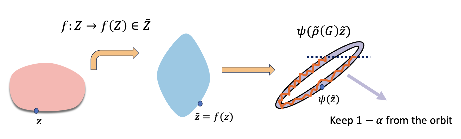
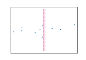
Figure 2: Left: A $1-\alpha$ prediction region extracted from the orbit of $\tilde{z}$, where $\tilde{z}=f(z)$. Right: A $95\%$-prediction region $T^{\mathrm{SymmPI}}(z_{1:10})$ for $z_{11}$ defined in (9). Here we let $z_{i}^{\top},i\in[11]$ be i.i.d. random vectors generated from $\mathcal{N}(0,20\cdot I_{2})$, where $I_{2}$ is the $2\times 2$ identity matrix. The blue stars represent 10 observed values, while the white region is the $95\%$-prediction region, as defined in Equation (9). Thus, the pink region depicts the complement of the prediction region, which is “safe”, in the sense of not having blue stars with 95% probability. In contrast, the 95% prediction region constructed via conformal prediction is the whole two-dimensional space. Consequently, using conformal prediction does not yield any “safe” area; and is thus not informative here.

To take into account the observation function $\mathrm{obs}:\mathcal{Z}\to\mathcal{O}$, we can simply intersect the prediction region with the set of valid observations $\{z:\mathrm{obs}(z)=z_{\mathrm{obs}}\}$, defining the prediction set

$$T^{\mathrm{SymmPI}}(z_{\mathrm{obs}})=\{z\in\mathcal{Z}:\psi(f(z))\leqslant t_{f(z)},\,\mathrm{obs}(z)=z_{\mathrm{obs}}\}.$$ (5)

This predictive inference method is applicable when the data has distributional invariance or symmetry, thus we call it SymmPI. See Figure 2 for an illustration. This method predicts a set of plausible values for the full data $z$. However, we are of course interested in a prediction set for the unobserved component of $z$. Usually, we can write this unobserved component as some function $m(z)$ of the data $z$, where $m:\mathcal{Z}\to\mathcal{U}$ for some space $\mathcal{U}$; and moreover such that $z$ is in a one-to-one correspondence with $(z_{\mathrm{obs}},m(z))$. In that case, $T^{\mathrm{SymmPI}}$ is equivalent to a prediction set for the unobserved component $m(z)$ of $z$. For instance, when $z=(z_{1},\ldots,z_{n},z_{n+1})^{\top}$ consists of $n+1$ datapoints, and the observation function takes values $\mathrm{obs}(z)=(z_{1},\ldots,z_{n})^{\top}$, then we can take $m(z)=z_{n+1}$.

4.2 Theoretical Properties

In this section we study the theoretical properties of our method.

4.2.1 Coverage Guarantee

We aim to control the coverage probability $P(Z\in T^{\mathrm{SymmPI}}(Z_{\mathrm{obs}}))$, ensuring it is at least $1-\alpha$. In order to achieve exact coverage $1-\alpha$, it is well-known that one may in general need to add a bit of randomization for discrete-valued data (Vovk et al., 2005). We now show how this idea can be generalized to our setting.

Definition 4.1 (Randomized SymmPI Prediction Set).

For $\tilde{z}\in\tilde{\mathcal{Z}}$, let $F_{\tilde{z}}$ be the cumulative distribution function (c.d.f.) of the random variable $\psi(\tilde{\rho}(G)\tilde{z}),\,G\sim U$, and $F^{\prime}_{\tilde{z}}$ be the probability it places on individual points, i.e., for $x\in\mathbb{R}$, $F^{\prime}_{\tilde{z}}(x)=F_{\tilde{z}}(x)-F^{-}_{\tilde{z}}(x)$, where $F^{-}_{\tilde{z}}(x)=\lim_{y\to x,y<x}F_{\tilde{z}}(y)\geqslant 0$. Let $\Delta_{\tilde{z}}=0$ if $F_{\tilde{z}}^{\prime}(t_{\tilde{z}})=0$, and otherwise let $\Delta_{\tilde{z}}\in(0,1]$ be

$$\Delta_{\tilde{z}}=\frac{1-\alpha-F_{\tilde{z}}^{-}(t_{\tilde{z}})}{F_{\tilde{z}}^{\prime}(t_{\tilde{z}})}.$$ (6)

Consider a random variable $V\sim\mathrm{Unif}[0,1]$ independent of $Z$, and the randomized SymmPI prediction set

$$T_{r}(z_{\mathrm{obs}})=\bigl{(}\{z:\psi(f(z))<t_{f(z)}\}\cup\{z:\psi(f(z))=t_{f(z)},\,V<\Delta_{f(z)}\}\bigr{)}\cap\{z:\mathrm{obs}(z)=z_{\mathrm{obs}}\}.$$ (7)

Clearly, $T_{r}(z_{\mathrm{obs}})\subset T^{\mathrm{SymmPI}}(z_{\mathrm{obs}})$. Our first result, proved in Section 8.1, shows that the randomized prediction set $T_{r}$ has coverage exactly $1-\alpha$, and the deterministic prediction set $T^{\mathrm{SymmPI}}$ has at least $1-\alpha$ and at most a bit higher, depending on the “jumps” $F^{\prime}_{\tilde{z}}$ in the distribution of $\psi(\tilde{\rho}(G)\tilde{z}),\,G\sim U$; generalizing results from conformal prediction (Vovk et al., 2005; Lei et al., 2013).

Theorem 4.2 (Coverage guarantee under distributional invariance).

For some group $\mathcal{G}$ with a uniform probability measure $U$, let the full data $Z\in\mathcal{Z}$ satisfy the distributional invariance property $Z=_{d}\rho(G)Z$ when $G\sim U$, for some action $\rho$ of the group $\mathcal{G}$ on $\mathcal{Z}$. Consider $\alpha\in[0,1]$, a space $\tilde{\mathcal{Z}}$, a $\mathcal{G}$-distributionally equivariant function $f:\mathcal{Z}\to\tilde{\mathcal{Z}}$ as per Definition 2.2, and a map $\psi:\tilde{\mathcal{Z}}\to\mathbb{R}$. Let the observed data be $Z_{\mathrm{obs}}=\mathrm{obs}(Z)$, for an observation function $\mathrm{obs}:\mathcal{Z}\to\mathcal{O}$ and some space $\mathcal{O}$. Then the SymmPI prediction region from (5), and the randomized prediction region from (7) have valid coverage, lower bounded by $1-\alpha$, and also—with $F^{\prime}$ from Definition 4.1—upper bounded as

$$1-\alpha=P(Z\in T_{r}(Z_{\mathrm{obs}}))\leqslant P(Z\in T^{\mathrm{SymmPI}}(Z_{\mathrm{obs}}))\leqslant 1-\alpha+\mathbb{E}[F^{\prime}_{f(Z)}(t_{f(Z)})].$$ (8)

There are various conditions under which we can upper bound the slack $\mathbb{E}[F^{\prime}_{f(Z)}(t_{f(Z)})]$ in the coverage error. For instance, if $F^{\prime}_{\tilde{z}}(x)\leqslant\tau$ for all $x\in\mathbb{R}$ and $\tilde{z}\in\tilde{\mathcal{Z}}$, then the coverage is at most $1-\alpha+\tau$. To be more concrete, consider the set $\mathcal{H}_{\tilde{z}}=\{g\in\mathcal{G}:\psi(\tilde{\rho}(g)\tilde{z})=\psi(\tilde{z})\}$ consisting of the group elements that fix $\psi(\tilde{z})$ under the action $\tilde{\rho}$. As we show, the size of this set controls the jumps in $F_{\tilde{z}}$, under the algebraic condition that $\mathcal{H}_{\tilde{z}}$ is a subgroup of $\mathcal{G}$. Recall that a set $\mathcal{H}\subset\mathcal{G}$ is a subgroup of $\mathcal{G}$, if $\mathcal{H}$ is also a group; this is denoted by $\mathcal{H}\leq\mathcal{G}$.

In particular, we will see in examples that often there is a set $\Omega\subset\tilde{\mathcal{Z}}$ such that $P(f(Z)\in\Omega)=1$ and such that for every $\tilde{z}^{\prime},\tilde{z}^{\prime\prime}\in\Omega$, $\mathcal{H}_{\tilde{z}^{\prime}}=\mathcal{H}_{\tilde{z}^{\prime\prime}}$. Then for $\mathcal{H}=\{g:\psi(\tilde{\rho}(g)\tilde{z})=\psi(\tilde{z}),\,\text{ for all }\tilde{z}\in\Omega\}$, we have $\mathcal{H}_{\tilde{z}^{\prime}}=\mathcal{H}$. It readily follows that $\mathcal{H}_{\tilde{z}^{\prime}}=\mathcal{H}$ is a subgroup of $\mathcal{G}$. Recalling that for a finite set $A$, we let $|A|$ be the number of elements—cardinality—of $A$, we have the following result:

Proposition 4.3 (Coverage upper bound).

If $\mathcal{G}$ is finite, and if for all $g\in\mathcal{G}$ the set $\mathcal{H}_{\tilde{z}}=\{g:\psi(\tilde{\rho}(g)\tilde{z})=\psi(\tilde{z})\}$ is a subgroup of $\mathcal{G}$, then $P(Z\in T^{\mathrm{SymmPI}}(Z_{\mathrm{obs}}))\leqslant 1-\alpha+\mathbb{E}|\mathcal{H}_{f(Z)}|/|\mathcal{G}|.$ In particular, if there is a set $\Omega\subset\tilde{\mathcal{Z}}$ such that $P(f(Z)\in\Omega)=1$ and such that for every $\tilde{z}^{\prime},\tilde{z}^{\prime\prime}\in\Omega$, $\mathcal{H}_{\tilde{z}^{\prime}}=\mathcal{H}_{\tilde{z}^{\prime\prime}}$, then for $\mathcal{H}=\{g:\psi(\tilde{\rho}(g)\tilde{z})=\psi(\tilde{z}),\,\text{ for all }\tilde{z}\in\Omega\}$, we have

$$P(Z\in T^{\mathrm{SymmPI}}(Z_{\mathrm{obs}}))\leqslant 1-\alpha+|\mathcal{H}|/|\mathcal{G}|.$$

See Section 8.2 for the proof. As we will see below, in many applications of interest, $\mathcal{H}_{\tilde{z}}$ are indeed subgroups of $\mathcal{G}$ for all $\tilde{z}$, and often $\mathcal{H}_{\tilde{z}}$ does not depend on $\tilde{z}$. In particular, in this case $|\mathcal{G}|/|\mathcal{H}|$ is the number of cosets of the subgroup $\mathcal{H}$ in $\mathcal{G}$. Thus the above general result gives a group-theoretic characterization of the slack in the coverage error. We now give examples of our framework.

Example 4.4 (Conformal prediction).

Continuing the example of exchangeable data from Section 2.2.1, we can recover results from conformal prediction (Gammerman et al., 1998; Vovk et al., 2005), by taking some space $\tilde{\mathcal{Z}}_{0}$, the $n+1$-fold product $\tilde{\mathcal{Z}}_{0}^{n+1}$, $\mathcal{Z}=\mathcal{Z}_{0}^{n+1}$, $\mathcal{G}=\mathrm{S}_{n+1}$ and $\rho$ as the permutation action. Further, we can let $\tilde{\mathcal{Z}}=\mathbb{R}^{n+1}$, and let $\mathrm{S}_{n+1}$ also act on $\tilde{\mathcal{Z}}$ by the permutation action. In an unsupervised case, we can take the observation function $\mathrm{obs}(z)=(z_{1},\ldots,z_{n})^{\top}$, for all $z$. In a supervised case where $z=((x_{1},y_{1}),\ldots,(x_{n+1},y_{n+1}))^{\top}$, we can take the observation function $\mathrm{obs}(z)=((x_{1},y_{1}),\ldots,(x_{n},y_{n}),x_{n+1})^{\top}$, for all $z$.

We set $f:\mathcal{Z}\to\tilde{\mathcal{Z}}$ as any permutation-equivariant map with respect to the permutation actions. Here $s(z_{j}):=s(z_{j};z):=[f(z)]_{j}$ are the non-conformity scores. Considering the supervised case for concreteness, we can take $\psi(\tilde{z})=\tilde{z}_{n+1}$ to be the last coordinate. Since $z$ decomposes as $z=(\mathrm{obs}(z),y_{n+1})$, a prediction set for $z$ is equivalent to a prediction set for $y_{n+1}$.

Clearly, $T^{\mathrm{SymmPI}}$ from (4) reduces to $s(Z_{n+1})\leqslant Q_{\beta^{\prime}}(s(Z_{1}),\ldots,s(Z_{n}))$, where $\beta^{\prime}=\lceil(n+1)(1-\alpha)\rceil/n$. This is identical to a standard conformal prediction set with non-conformity score $s$. If $Z$ has exchangeable coordinates, Theorem 4.2 recovers the classical conformal coverage lower bound $P(s(Z_{n+1})\leqslant Q_{1-\alpha}(s(Z_{1}),\ldots,s(Z_{n+1})))\geqslant 1-\alpha$ from Gammerman et al. (1998); Vovk et al. (2005).

Then, note that for $g\in\mathrm{S}_{n+1}$, $(\tilde{\rho}(g)\tilde{z})_{n+1}=\tilde{z}_{g^{-1}(n+1)}$. Hence, $\mathcal{H}_{\tilde{z}}=\{g:\tilde{z}_{g^{-1}(n+1)}=\tilde{z}_{n+1}\}$. If all coordinates of $\widetilde{Z}$ are distinct—which holds with probability one if $f$ is injective and $(Z_{1},\ldots,Z_{n+1})$ has a continuous distribution—then $\mathcal{H}_{\tilde{z}}=\mathcal{H}=\{g:g(n+1)=n+1\}$ is the stabilizer of the $(n+1)$st element, the subgroup of permutations fixing the last coordinate. In this case, $|\mathcal{H}|/|\mathcal{G}|=n!/(n+1)!=1/(n+1)$, and we recover the classical result that the over-coverage of conformal prediction is at most $1/(n+1)$ (Lei et al., 2013).

Example 4.5 (Coordinate-independent data).

Continuing the example of coordinate-independent data from Section 2.2.1, we can work in the same setting as above, except letting $\mathcal{Z}_{0}=\mathbb{R}^{p}$, while the group is the direct product $\mathcal{G}=\mathrm{S}_{n+1}\times\mathrm{O}(p)$, acting on $z=(z_{1}^{\top},\ldots,z_{n+1}^{\top})^{\top}\in(\mathbb{R}^{p})^{n+1}$ via the action $\rho(\pi,O)z=((Oz_{\pi^{-1}(1)})^{\top},\ldots,(Oz_{\pi^{-1}(n+1)})^{\top})^{\top}$. For the non-conformity score $s:\mathcal{Z}_{0}\to\mathbb{R}$, we may aim to predict how close a new object could come to the the trajectory of another celestial body of interest; say, the path of a rocket.

For instance, consider the locus $z_{n+1,1}=0$ and suppose we aim to predict a region $|z_{n+1,1}|\geqslant C$ that contains the next observation at least $1-\alpha$ of the time. Then we can take $s(z_{n+1})=-|z_{n+1,1}|$, and the prediction set for the $(n+1)$st observation becomes

$$T^{\mathrm{SymmPI}}(z_{1:n})=\{z_{n+1}:-|z_{n+1,1}|\leqslant Q_{1-\alpha}\left(-|(Oz_{\pi^{-1}(n+1)})_{1}|,\,O\sim U(\mathrm{O}(p)),\pi\sim U(\mathrm{S}_{n+1})\right)\}.$$ (9)

This can be further simplified since for any $v$, $(Ov)_{1}=_{d}W^{\top}v/\|W\|_{2}$, where $W\sim\mathcal{N}(0,I_{p})$ and $\|W\|_{2}$ is the Euclidean norm of $W$. For illustration, we present a two-dimensional toy example in Figure 2 (right). In this case, the prediction set can be interpreted as “we are 95% sure that a new observation $Z_{n+1}$ will have $|Z_{n+1,1}|$ at least this large”. Such a region may be useful to determine the allowable range of motion of a rocket moving along the vertical axis—there is 95% chance that the next celestial body outside of the vertical strip.

We also mention that a split, or split-data, version of SymmPI—inspired by inductive or split conformal prediction (Papadopoulos et al., 2002)—is a special case of our method. Let the full data be given by $Z=(Z_{\mathrm{tr}},Z^{\prime})^{\top}$, where $Z_{\mathrm{tr}}$ consists of training data, and $Z^{\prime}$ consists of calibration and test data. Suppose that for some group $\mathcal{G}_{0}$, the distribution of $Z^{\prime}$ conditional on $Z_{\mathrm{tr}}$ is $\mathcal{G}_{0}$-invariant. Then, we can use the methodology described above, applied to $Z^{\prime}$ and $\mathcal{G}_{0}$ instead of $Z$ and $\mathcal{G}$. This procedure has valid coverage even when the $\mathcal{G}_{0}$-distributionally equivariant map $f$ is not fixed as above, but is learned using $Z_{\mathrm{tr}}$. The key advantage compared to full SymmPI  is that we can fit $f$ once on $Z_{\mathrm{tr}}$, and then use it as a fixed predictor on $Z^{\prime}$; which can improve computational efficiency compared to SymmPI. For $f$ to be a useful predictor, it is beneficial if $Z_{\mathrm{tr}}$ and $Z^{\prime}$ have a similar structure. For instance, this could be the case if $Z_{\mathrm{tr}}$ also satisfies $\mathcal{G}_{0}$-equivariance.

Finally, we mention that, while our results only require $f$ to be distributionally equivariant, in practice there are often more known examples of deterministically equivariant functions, and so we will typically still take $f$ to be deterministically equivariant. However, we believe that our theoretical contribution of introducing distributional equivariance is fundamental, because it reflects a broad condition under which distributional invariance is preserved under compositions. Thus it is a crucial notion for predictive inference methods based on symmetry.

4.2.2 Extension: Distribution Shift

Next, we present an extension of our coverage result for the case of distribution shift. To present this result, we need to recall some additional notions. For the subgroup $\mathcal{H}\leq\mathcal{G}$ the set $g\mathcal{H}=\{gh:h\in\mathcal{H}\}$ is called a (left) coset of $\mathcal{H}$ in $\mathcal{G}$. The set of cosets is denoted as $\mathcal{G}/\mathcal{H}:=\{g\mathcal{H}:g\in\mathcal{G}\}$. Then $\mathcal{G}$ is partitioned into cosets $g\mathcal{H}$, and we obtain a set $S$ of representatives of cosets in $\mathcal{G}/\mathcal{H}$ by choosing an element of each coset.

First, we allow for a distribution shift away from distributional invariance, i.e., $Z\neq_{d}\rho(G)Z$. We provide a general coverage bound for this scenario. For $g\in\mathcal{G}$, define the map $\ell_{g}:\tilde{\mathcal{Z}}\to\mathbb{R}$ such that for all $\tilde{z}\in\tilde{\mathcal{Z}}$, $\ell_{g}(\tilde{z})=\psi(\tilde{\rho}(g)\tilde{z})$. Let $\mathcal{F}=\{\ell_{g},\,g\in\mathcal{G}\}$ be the set of all maps $\ell_{g}$, $g\in\mathcal{G}$. Now, $\mathcal{H}=\{g:\ell_{g}=\ell_{e}\}$ is clearly a subgroup of $\mathcal{H}$. Hence, $\mathcal{G}$ is partitioned into cosets $g\mathcal{H}$, corresponding to distinct values of $\ell_{g}$. Let $U(\mathcal{G}/\mathcal{H})$ be the invariant probability measure over the cosets (Nachbin, 1976, Corollary 4, p. 140); and identify $\mathcal{G}/\mathcal{H}$ with a measurably chosen set $S$ of representatives. Let $G^{\prime}\sim U(\mathcal{G}/\mathcal{H})$, identified with a random variable over $S$. For instance, for a finite $\mathcal{G}$, we can identify $U(\mathcal{G}/\mathcal{H})$ with the uniform distribution over a set of representatives $\{g_{1},\ldots,g_{|\mathcal{F}|}\}$ of the cosets $\mathcal{G}/\mathcal{H}$. For any $\tilde{z}\in\tilde{\mathcal{Z}}$, define $\nu(\tilde{z})=\psi(\tilde{z})-t_{\tilde{z}}$ and, with TV denoting total variation distance,

$$\Delta=\mathbb{E}_{G^{\prime}\sim U(\mathcal{G}/\mathcal{H})}\textrm{TV}_{Z}\Big{(}\nu(f(Z)),\nu(\tilde{\rho}(G^{\prime})f(Z))\Big{)}.$$ (10)

See Section 8.4 for the proof of the following result.

Theorem 4.6 (Coverage guarantee under distribution shift).

Under the conditions of Theorem 4.2, even if $Z$ does not necessarily satisfy distributional invariance, we have with $\Delta$ from (10) that

$$-\Delta\leqslant P\Big{(}Z\in T^{\mathrm{SymmPI}}(Z_{\mathrm{obs}})\Big{)}-(1-\alpha)\leqslant\Delta+\mathbb{E}[F^{\prime}_{f(Z)}(t_{f(Z)})].$$ (11)

Theorem 4.6 establishes that, even if $Z\neq_{d}\rho(G)Z$, we can derive coverage bounds similar to those found in Theorem 4.2, up to a margin of $\Delta$ as given in equation (10). This gap reduces to zero when the distributional invariance property holds (i.e., $Z=_{d}\rho(G)Z$), in which case $\Delta=0$.

The aforementioned result relies on symmetry in two ways. First, the quantile $t_{\tilde{z}}$ in equation (4) is chosen for the uniform probability distribution over the group; or equivalently over representatives of cosets. Second, the function $f$ is required to be distributionally equivariant with respect to $\mathcal{G}$. In Section 7.2, we introduce a novel algorithm for scenarios where the aforementioned two symmetry properties do not hold. We also provide theoretical coverage guarantees for this algorithm. Notably, our framework recovers the results presented in Theorems 2 and 3 of Barber et al. (2023) as a special case, in the context of studying conformal prediction with the group $\mathcal{G}=S_{n+1}$ and the function $\psi$ with $\psi(z)=z_{n+1}$ for all $z$. For more details, we refer to Section 7.2.

4.3 Computational Considerations

In this section, we discuss computational considerations for our prediction regions. Given $f$ and $\psi$, we need to compute the set in (5), i.e., $\mathrm{obs}^{-1}(z_{\mathrm{obs}})\cap\{z:\psi(f(z))\leqslant t_{f(z)}\}$, where $\mathrm{obs}^{-1}(z_{\mathrm{obs}})$ denotes the preimage of $z_{\mathrm{obs}}$ under the map $\mathrm{obs}$, for a given $z_{\mathrm{obs}}$. Often, the preimage of the observation map can be characterized in a convenient way; in many cases the observation map selects a subset of the coordinates of $z$, and so its preimage includes the set of observations with all possible values of the missing coordinates.

Moreover, we can write the second set of the above intersection as a preimage under $f$ in the form $f^{-1}(B)$, where $B=\{\tilde{z}\in\tilde{\mathcal{Z}}:\psi(\tilde{z})\leqslant t_{\tilde{z}}\}$. A key step to compute $B$ is to compute the quantiles $t_{\tilde{z}}$ over the randomness of $G\sim U$, or—following notation from Section 4.2.2—$G^{\prime}\sim U(\mathcal{G}/\mathcal{H})$. When the number of equivalence classes $\mathcal{G}/\mathcal{H}$ is not large, we can calculate the quantile by enumeration. However, if the number of equivalence classes is large, a practical approach is to sample from each equivalence class to approximate the quantile Specifically, we can define

$$\tilde{t}_{\tilde{z}}:=Q_{1-\alpha}\left(\psi(\tilde{\rho}(G_{1})\tilde{z}),\psi(\tilde{\rho}(G_{2})\tilde{z}),\cdots,\psi(\tilde{\rho}(G_{M})\tilde{z})\right),$$ (12)

where $G_{1},\cdots,G_{M}$ are sampled independently from $U(\mathcal{G}/\mathcal{H})$. We then define the prediction set

$$\tilde{T}^{\mathrm{SymmPI}}(z_{\mathrm{obs}}):=\{z\in\mathcal{Z}:\psi(f(z))\leqslant\tilde{t}_{f(z)},\,\mathrm{obs}(z)=z_{\mathrm{obs}}\}.$$

This has the following coverage guarantee, with a proof deferred to Section 8.3.

Proposition 4.7.

Under the conditions of Theorem 4.2, we have $P(Z\in\tilde{T}^{\mathrm{SymmPI}}(Z_{\mathrm{obs}}))\geqslant 1-\alpha.$

For the remaining problems, i.e., computing $A$ and finding its preimage under $f$, at the most general level, various approaches can be employed to generate suitable approximate solutions. At the highest level of generality, similar computational problems arise in standard conformal prediction, and no general computational approaches are known. Our setting is similar, and thus computational approaches must be designed on a case by case basis. In many cases of interest, including all those presented in the paper, the computational problem simplifies and can be solved conveniently. One approximate method involves systematically examining a grid of candidate values of $\tilde{z}$, and retaining those for which $\psi(\tilde{z})\leqslant t_{\tilde{z}}$. Further, if we can choose $f$ to be an invertible function whose inverse is convenient to compute, then the preimage under $f$ can be convenient to find. Otherwise, in general, one may need to search over a grid on $\mathcal{Z}$ (instead of $\tilde{\mathcal{Z}}$) to approximate $f^{-1}(A)$.

4.4 Illustration Revisited: Graphs

In this section, we discuss an illustration of our methods for random variables whose symmetries are captured by a graph. We discuss properties for prediction sets and finally use a simple tree example to present these concepts.

We focus on a dataset denoted as $Z=(Z_{1},\ldots,Z_{n+1})^{\top}\in\tilde{\mathcal{Z}}_{0}^{n+1}$, for some set $\tilde{\mathcal{Z}}_{0}$, typically $\mathbb{R}^{p}$ for some positive integer $p$. The symmetries of $Z$ are described by the automorphism group $\mathcal{G}=\mathrm{Aut}(A)$ of a graph, as described in Section 2.2.1. If it is feasible to enumerate the automorphism group, then we can use the prediction set from (5). However, in general determining the automorphism of a graph is a hard problem; see e.g., Babai (2016) for the related graph automorphism problem. We discuss a coarsening approach to partially overcome this in Section 7.3.

4.4.1 Properties of Prediction Sets for Graphs, and Tree-structured Graphical Model

In this section, we briefly discuss the properties of prediction sets for graphs. In the prediction set from (5), we consider some space $\tilde{\mathcal{Z}}_{0}$, the $n+1$-fold product $\tilde{\mathcal{Z}}_{0}^{n+1}$, take $\mathcal{Z}=\tilde{\mathcal{Z}}=\tilde{\mathcal{Z}}_{0}^{n+1}$, $f:\mathcal{Z}\to\mathcal{Z}$ as the identity, and $\rho,\tilde{\rho}$ to be permutation actions. We can take $\psi$ such that $\psi(z)=z_{n+1}$ for all $z$, in which case we are predicting $z_{n+1}$ in a graph. Let $\mathcal{H}_{n+1}$ be the stabilizer subgroup of $n+1$ in $\mathcal{G}$, i.e., $\mathcal{H}_{n+1}=\{g\in\mathcal{G}:g(n+1)=n+1\}$. Let $b=|\mathcal{G}/\mathcal{H}_{n+1}|$ be the number of equivalence classes of the quotient $\mathcal{G}/\mathcal{H}_{n+1}$ and take a collection $g_{1},\ldots,g_{b}\in\mathcal{G}$ of representatives of the equivalence classes. By the orbit-stabilizer theorem (Artin, 2018, Proposition 6.8.4), $B=\{g_{1}(n+1),\ldots,g_{b}(n+1)\}\subset[n+1]$ is the orbit of $n+1$ under $\mathcal{G}$ acting on $[n+1]$. Then, for $\tilde{z}\in\tilde{\mathcal{Z}}_{0}^{n+1}$, the quantile $t_{\tilde{z}}$ is presented as $Q_{1-\alpha}(\{\tilde{z}_{j},$ $j\in B\})$. As a special case, when $\mathcal{G}=\mathrm{S}_{n+1}$, the orbit of $n+1$ is all of $[n+1]$. Then the quantile reduces to the one used in standard conformal prediction.

There are many other choices of $\psi$. Suppose for simplicity that $\mathcal{Z}_{0}=\mathbb{R}$. Then, we can take for example $\psi(z)=(e_{n+1}-1_{n+1}/(n+1))^{\top}z$ for all $z\in\mathcal{Z}$, which measures the difference between the unknown element $z_{n+1}$ and the grand mean. Alternatively, $\psi(x)=(e_{n+1}-1_{B}/b)^{\top}x$ for all $x$ measures the difference between the unknown value and the average of its orbit.

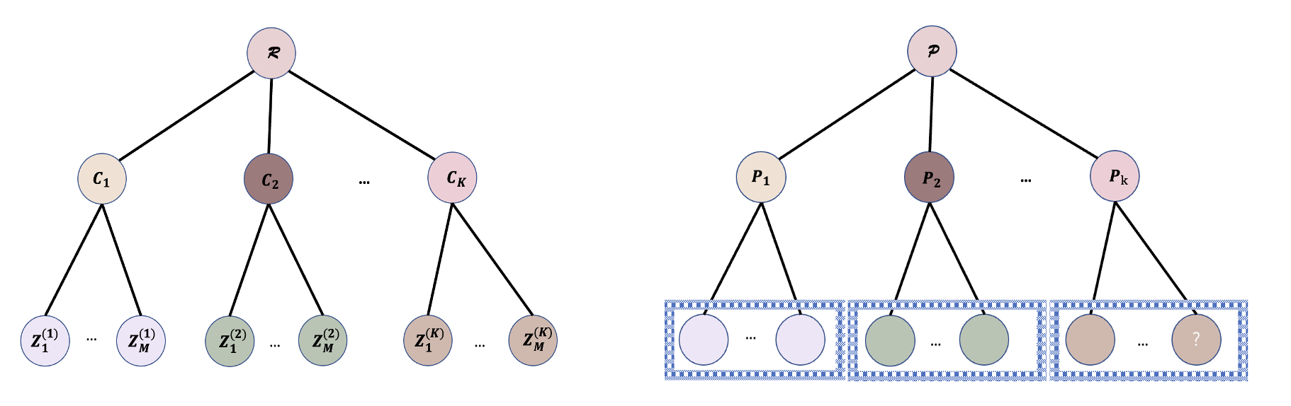
Figure 3: Left: Example of a depth-two tree-structured graphical model. Right: Example of a two-layer hierarchical model.

Next, we use a simple tree-structured graphical model example to showcase the above properties; see Figure 3. The rooted tree $\Gamma$ has a root with an associated random variable $R$. The root has $K\geqslant 1$ children, which are associated with random variables $C_{1}\ldots,C_{K}$ at its first layer; these define $K$ branches. Each of the nodes $C_{k}$, $k\in[K]$ in the first layer has $M\geqslant 1$ children with associated random variables $Z_{1}^{(k)},\ldots,Z_{M}^{(k)}$ in the second layer. We assume that in the associated graph describing the symmetry, each node is connected precisely to its children. Then, we assume that the joint distribution of the random vector $T=(R,C_{1}\ldots,C_{K},Z_{1}^{(1)},\ldots,Z_{M}^{(K)})^{\top}\in\mathcal{Z}$ associated with this depth-two tree satisfies $g\cdot\Gamma=_{d}\Gamma$, where $g$ is any element in the automorphism group $\mathcal{G}$, represented as a subgroup of $\mathrm{S}_{n+1}$.

We can consider the setting when $Z_{M}^{(K)}$, the last node of the last branch, is unobserved, and suppose for simplicity that $\mathcal{Z}_{0}=\mathbb{R}$. We can let $\psi(z)=|e_{1+K+K\cdot M}^{\top}z|$, with $z\in\mathcal{Z}$. The orbit of $e_{1+K+K\cdot M}^{\top}$ is $\{e_{1+K+i}^{\top},i\in[K\cdot M]\}$. Therefore, the quantiles from (4) are $t^{(1)}_{z}:=Q_{1-\alpha}(|z_{1}^{(1)}|,\ldots,|z_{M}^{(K)}|)$, and the prediction set with $1-\alpha$ probability coverage reduces to

$$T^{\mathrm{SymmPI}}(z_{\mathrm{obs}})=\{z:|z_{M}^{(K)}|\leqslant t^{(1)}_{z},\,\mathrm{obs}(z)=z_{\mathrm{obs}}\}.$$

We can also aim to predict at a cluster after coarsening the graph, and we describe this in Section 7.3.

5 Two-layer Hierarchical Model

This section is devoted to studying data with a two-layer hierarchical structure. Different from the tree-structured graphical model example from Section 4.4.1, here the zeroth- and first-layer nodes are not observed. Such a model can be useful in many applications, such as meta-learning (Fisch et al., 2021; Park et al., 2022), sketching (Sesia et al., 2023), and clustered data (Dunn et al., 2022; Lee et al., 2023).

5.1 Problem Setting

In a two-layer hierarchical model, for the first-layer nodes, we draw distributions $P_{k}\sim\mathcal{P},k\in[K]$ independently from a distribution $\mathcal{P}$. These can be viewed as specifying distinct sub-populations from which data is collected. From the perspective of meta-learning, they can be viewed as distinct but related tasks (e.g., prediction in various environments). The second-layer nodes (or leaves for simplicity) in the $k$-th branch are random variables $Z_{i}^{(k)},i\in[M]$ drawn exchangeably from the distribution $P_{k},k\in[K]$ (Dunn et al., 2022; Park et al., 2022; Lee et al., 2023). An illustration is presented in the right panel of Figure 3. Our goal is to construct prediction sets for both unsupervised and supervised settings, given as follows:

Example 5.1 (Unsupervised Learning).

We let $Z_{i}^{(k)}\in\mathbb{R}$, $i\in[M]$, $k\in[K]$.

Example 5.2 (Supervised Learning).

For some space $\mathcal{Z}_{0}$, we let $Z_{i}^{(k)}=(X_{i}^{(k)},Y_{i}^{(k)})\in\mathcal{Z}_{0},i\in[M]$, $k\in[K]$, and suppose that $Y_{i}^{(k)}=\mu_{P_{k}}(X_{i}^{(k)})+\varepsilon_{i}^{(k)},i\in[M]$, where $\varepsilon_{i}^{(k)},i\in[M]$ are i.i.d. zero-mean random variables whose distributions may depend on $P_{k},k\in[K]$.

Let us consider the set $[KM]=\{1,\ldots,KM\}$ and for each $a\in[KM]$, where $a=(k-1)\cdot M+i$ for a unique $i\in[M]$, $k\in[K]$, associate with $a$ the random variable $Z_{i}^{(k)}\in\mathbb{R}$. Thus the random variables $Z_{i}^{(k)}\in\mathbb{R}$, $i\in[M]$ in the $k$-th branch are associated with the block $b_{k}=\{(k-1)\cdot M+i,i\in[M]\}$. We let $\Lambda_{K,M}\subset\mathrm{S}_{[KM]}$ be the group of $KM$-permutations that map each block $b_{k}$ into some other block $b_{k^{\prime}}$ in a bijective way. Then for both the unsupervised and supervised cases, the distribution of the data is $\Lambda_{K,M}$-invariant.

We aim to build prediction sets for some unknown components of the last branch, hoping to improve prediction by pooling information both within and across branches. We explain our steps next.

5.2 Methodological Considerations for Unsupervised Learning

In this section, we develop our methodology for building prediction sets in the unsupervised case. For all $k\in[K]$, define $\bar{Z}_{k}=\sum_{j=1}^{M}Z_{j}^{(k)}/M$, $\hat{\sigma}_{k}^{2}=1$ if $M=1$,

$$\hat{\sigma}_{k}^{2}=\frac{\sum_{j=1}^{M}(Z_{j}^{(k)}-\bar{Z}_{k})^{2}}{M-1}$$

otherwise, and $\bar{Z}=\sum_{k=1}^{K}\bar{Z}_{k}/K$. For some constant $c\geqslant 0$, and for all $k\in[K]$, define the events $A_{k,c}=\{|\bar{Z}_{k}-\bar{Z}|\leqslant c\hat{\sigma}_{k}/\sqrt{M}\}$. These capture the events that the means of the elements within the $k$-th branch are close to the grand mean. Let $A_{k,c}^{\complement}$ be the complement of $A_{k,c}$, and $I(A)$ be the indicator function of an event $A$, which equals $I(A)=1$ if $A$ happens, and $I(A)=0$ otherwise. We also define, for all $k\in[K],i\in[M]$,

$$\tilde{Z}_{i}^{(k)}:=\frac{|Z_{i}^{(k)}-[\bar{Z}I(A_{k,c})+\bar{Z}_{k}I(A_{k,c}^{\complement})]|}{\hat{\sigma}_{k}},$$ (13)

which are the standardized absolute deviations of $Z_{i}^{(k)}$ from the grand mean if the branch mean is close to that, or to branch mean itself otherwise. Here $c$ is an absolute constant that can be set as $c=2$, as an approximate 97.5% quantile of the standard Gaussian distribution. As explained later, it can potentially also be optimized by minimizing a prediction loss. In Section 7.4.1 of the Appendix, we explain how $(\tilde{z}_{i}^{(k)})_{k\in[K],i\in[M]}=:f(z)$ can be obtained as functions of $z$ via a fixed message-passing graph neural network $f$ on a graph obtained by constructing proxy statistics for the nodes in the zeroth- and first-layer nodes (also detailed below for the supervised case). We construct the prediction region (5) for $Z_{M}^{(K)}$ by using that $\widetilde{Z}$ is $\Lambda_{K,M}$-distributionally invariant.

To understand our procedure, suppose for a moment that $P_{k},k\in[K]$ have finite expectations $\mu_{k},k\in[K]$; but we emphasize that our method does not require this condition. When some branch means $\bar{Z}_{k}\approx\mu_{k},k\in[K]$ and $\bar{Z}\approx\sum_{j=1}^{K}\mu_{j}/K$ are very different—i.e., on the event $A_{k,c}^{\complement}$—our procedure centers observations within those branches by estimating the within-branch means $\mu_{k},k\in[K]$. On the other hand, when $\bar{Z}_{k}\approx\bar{Z}$ holds for all branches $k\in[K]$—i.e., on $A_{k,c}$—we pool all observations and mimic standard conformal inference. Therefore, our procedure interpolates prediction sets built using each individual branch and prediction sets built using full standard conformal inference.

We let $J_{K,M}=[M]\times[K]\setminus\{(M,K)\}$ denote the indices of the fully observed datapoints. The following result formalizes the coverage guarantee of our result:

Proposition 5.3.

If the data $Z$ follows the two-layer hierarchical model introduced at the beginning of Section 5.1, and the observation function has values $\mathrm{obs}(z)=(z_{i}^{(k)})_{(i,k)\in J_{K,M}}$ for all $z$, then the prediction set for $Z_{M}^{(K)}$ from (5) with $\psi(\tilde{z})=\tilde{z}_{M}^{(K)}$ and $t_{\tilde{z}}=Q_{1-\alpha}((\tilde{z}_{i}^{(k)})_{k=1,i=1}^{K,M})$ has coverage at least $1-\alpha$. Moreover, if $\widetilde{Z}$ has a continuous distribution, then the coverage is at most $1-\alpha+1/(KM)$.

The proof of Proposition 5.3 is deferred to Section 8.5. We compare our method with alternatives in Section 5.4.

5.3 Methodology Considerations for Supervised Learning

In this section, we consider the two-layer hierarchical model in a supervised learning setting. To ease the computational burden, we adopt split predictive inference. For every branch $k\in[K]$, we set the first $M^{\prime}$—approximately half—datapoints to be the training sample, and let $Z_{\operatorname{tr}}$ be the training data gathered from all branches. We fit $\hat{\mu}(\cdot;Z_{\operatorname{tr}}):\mathbb{R}\to\mathbb{R}$ based on $Z_{\operatorname{tr}}$, such that $x\mapsto\hat{\mu}(x;Z_{\operatorname{tr}})$ is an estimator of the regression function in the pooled data. Further, for all branches, we fit $\hat{\mu}_{k}(\cdot;Z_{\operatorname{tr}}),k\in[K]$ based on $Z_{\operatorname{tr}}$, as estimators of the within-branch regression functions $\mu_{P_{k}}$ from Example 5.2.

Using $Z_{\operatorname{tr}}$, we also fit pointwise confidence bands $x\mapsto\hat{\sigma}_{k}(x;Z_{\operatorname{tr}}),k\in[K]$ by estimating the pointwise standard error of $x\mapsto\hat{\mu}_{k}(x;Z_{\operatorname{tr}}),k\in[K]$ over the randomness of the fitting process. Many classical estimators $\hat{\mu}_{k}(\cdot;Z_{\operatorname{tr}})$ have explicit expressions for standard error curves $\hat{\sigma}_{k}(\cdot;Z_{\operatorname{tr}})$, $k\in[K]$ including parametric models, non-parametric kernel regression, splines, etc. We emphasize that our method does not require any coverage properties for $\hat{\sigma}_{k}$.

Suppose that there are $M$ remaining datapoints in each branch, and without loss of generality, call them $(X_{i}^{(k)},Y_{i}^{(k)})$, $k\in[K]$, $i\in[M]$. For $k\in[K]$, $i\in[M]$, let

$$\bar{Z}_{i}^{(k)}=(Y_{i}^{(k)}-\hat{\mu}_{k}(X_{i}^{(k)};Z_{\operatorname{tr}}),Y_{i}^{(k)}-\hat{\mu}(X_{i}^{(k)};Z_{\operatorname{tr}}),\hat{\sigma}_{k}(X_{i}^{(k)};Z_{\operatorname{tr}})).$$

We require that $\bar{Z}=(\bar{Z}_{i}^{(k)})_{k\in[K],i\in[M]}$ is $\Lambda_{K,M}$-distributionally invariant. This follows if $Z=(Z_{\operatorname{tr}},$ $(Z_{i}^{(k)})_{k\in[K],i\in[M]})$ is $\Lambda_{K,M+M^{\prime}}$-distributionally invariant and the map $Z\mapsto\bar{Z}$ is $\Lambda_{K,M+M^{\prime}}$-distributionally equivariant. To ensure this, we use the same algorithm for training $\hat{\mu}_{k}(\cdot;Z_{\operatorname{tr}})$, $\hat{\sigma}_{k}(\cdot;Z_{\operatorname{tr}})$ in all branches $k\in[K]$, and ensure they are all invariant to the order of the data within branch $k$.

In what follows, we suppress the dependence of $\hat{\mu},\hat{\mu}_{k},\hat{\sigma}_{k}$ on the training data.

For all $k\in[K],i\in[M]$, define

$${\bar{Z}_{i}^{{}^{\prime}(k)}}=\bigg{[}Y_{i}^{(k)}-\hat{\mu}(X_{i}^{(k)})I\bigg{(}\bigg{|}\frac{\hat{\mu}_{k}(X_{i}^{(k)})-\hat{\mu}(X_{i}^{(k)})}{\hat{\sigma}_{k}(X_{i}^{(k)})}\bigg{|}\leqslant c\bigg{)}-\hat{\mu}_{k}(X_{i}^{(k)})I\bigg{(}\bigg{|}\frac{\hat{\mu}_{k}(X_{i}^{(k)})-\hat{\mu}(X_{i}^{(k)})}{\hat{\sigma}_{k}(X_{i}^{(k)})}\bigg{|}>c\bigg{)}\bigg{]}.$$ (14)

We set $\hat{\varepsilon}_{k}=1,$ for all $k\in[K]$ when $M=1$ and $\hat{\varepsilon}_{k}=\sqrt{\sum_{i=1}^{M}(\bar{Z}_{i}^{{}^{\prime}(k)})^{2}/(M-1)}$ otherwise.

Let $\widetilde{Z}=(\widetilde{Z}_{1},\ldots,\widetilde{Z}_{K})^{\top}$, where for all $k\in[K]$, $\widetilde{Z}_{k}=(\widetilde{Z}_{1}^{(k)},\ldots,\widetilde{Z}_{M}^{(k)})^{\top}$ and for all $k\in[K],i\in[M]$, we define the map $\bar{Z}\mapsto f(\bar{Z})=(f_{i}^{(k)}(\bar{Z}))_{i=1,k=1}^{M,K}$ via

$$\widetilde{Z}_{i}^{(k)}:=f_{i}^{(k)}(\bar{Z}):=\frac{\bar{Z}_{i}^{{}^{\prime}(k)}}{\hat{\varepsilon}_{k}}.$$ (15)

We now argue that if the data $\bar{Z}_{i}^{(k)},i\in[M]$, $k\in[K]$ are $\Lambda_{K,M}$-distributionally invariant, then $\widetilde{Z}$ also satisfies this property. To see this, we define a special fixed message-passing graph neural net computing $f$ on the two-layer tree from Figure 3 (right), which captures the invariances of $\bar{Z}$, mapping $\bar{Z}\mapsto\widetilde{Z}=f(\bar{Z})$. Since message-passing GNNs are equivariant, it will follow that $\widetilde{Z}$ is also $\Lambda_{K,M}$-distributionally invariant. In fact, our MPGNN operates only on the subgraph of the two-layer tree excluding the zeroth-layer node. The message passing GNN is defined in five steps:

• Step 1: We initialize the leaves $z_{i}^{(k,0)},i\in[M],k\in[K]$, to have three channels: $z_{i}^{(k,0)}=(z_{i,1}^{(k,0)},z_{i,2}^{(k,0)},z_{i,3}^{(k,0)})^{\top}$, where $z_{i,1}^{(k,0)}=y_{i}^{(k)}-\hat{\mu}_{k}(x_{i}^{(k)})$, $z_{i,2}^{(k,0)}=y_{i}^{(k)}-\hat{\mu}(x_{i}^{(k)})$, $z_{i,3}^{(k,0)}=\hat{\sigma}_{k}(x_{i}^{(k)})$. We initialize the first-layer nodes as all ones vectors with three channels: $p^{(k,0)}=(p_{1}^{(k,0)},p_{2}^{(k,0)}$, $p_{3}^{(k,0)})^{\top}$ $=(1,1,1)^{\top}$, $k\in[K]$.

• Step 2: Let the kernel $\mathbb{K}$ be defined by $\mathbb{K}(x)=I(|x|\leqslant c)$ for all $x$. We update each leaf individually as $z_{i}^{(k,1)}=f_{1}(z_{i}^{(k,0)})=(z_{i,1}^{(k,0)},z_{i,2}^{(k,0)},(z_{i,2}^{(k,0)}-z_{i,1}^{(k,0)})\cdot\mathbb{K}(|(z_{i,2}^{(k,0)}-z_{i,1}^{(k,0)})/z_{i,3}^{(k,0)}|))^{\top},i\in[M],k\in[K]$. This corresponds to taking the map $\lambda_{0}$ in (3) to only depend on its first input. The updated third coordinate becomes

  $$(z_{i,2}^{(k,0)}-z_{i,1}^{(k,0)})\cdot\mathbb{K}(|(z_{i,2}^{(k,0)}-z_{i,1}^{(k,0)})/z_{i,3}^{(k,0)}|)$$

  $$\quad=[\hat{\mu}(x_{i}^{(k)})-\hat{\mu}_{k}(x_{i}^{(k)})]\cdot I(|\hat{\mu}(x_{i}^{(k)})-\hat{\mu}_{k}(x_{i}^{(k)})|/\hat{\sigma}_{k}(x_{i}^{(k)})\leqslant c).$$

  We keep the values of the first-layer nodes unchanged: $p^{(k,1)}=p^{(k,0)}$, $k\in[K]$.

• Step 3: We update the leaves as $z_{i}^{(k,2)}=f_{2}(z_{i}^{(k,1)})=(|y_{i}^{(k)}-\hat{\mu}_{k}(x_{i}^{(k)})-z_{i,3}^{(k,1)}|,z_{i,2}^{(k,1)},z_{i,3}^{(k,1)})^{\top}$, $i\in[M],k\in[K].$ This also corresponds to a map $\lambda_{0}$ that only depends on its first input.

• Step 4: We update the first layer nodes as $p^{(k,2)}=(p_{1}^{(k,2)},1,1)^{\top},k\in[K]$, where $p_{1}^{(k,2)}=f_{32}(p^{(k,1)},\sum_{i=1}^{M}f_{31}(z_{i}^{(k,2)},p^{(k,1)}))$, and we have $f_{31}(x,y)=x^{2}/(M-1)$ and $f_{32}(x,y)=\sqrt{y}$. This corresponds to a standard message passing update in (3). Thus, after the update, we have $p^{(k,2)}=(\hat{\varepsilon}_{k},1,1)^{\top}$, where

  $$\hat{\varepsilon}_{k}=\sqrt{\frac{\sum_{i=1}^{M}\Big{(}z_{i,1}^{(k,2)}\Big{)}^{2}}{M-1}}$$

  for all $k\in[K]$. In this step, we fix the values of the leaves.

• Step 5: We update the leaves $z_{i}^{(k,3)}=f_{41}(z_{i}^{(k,2)},f_{42}(p^{(k,2)},z_{i}^{(k,2)}))$, where $f_{42}(p^{(k,2)},z_{i}^{(k,2)})=p^{(k,2)}$ and $f_{41}(z_{i}^{(k,2)},p^{(k,2)})=(z_{i,1}^{(k,2)}/p_{1}^{(k,2)}$, $z_{i,2}^{(k,2)}$, $z_{i,3}^{(k,2)})^{\top}$. Thus, $z_{i}^{(k,3)}=(|y_{i}^{(k)}-\hat{\mu}_{k}(x_{i}^{(k)})-z_{i,3}^{(k,1)}|/p_{1}^{(k,2)}$, $z_{i,2}^{(k,2)}$, $z_{i,3}^{(k,2)})^{\top}$, $i\in[M],k\in[K].$ The first entry, $z_{i,1}^{(k,2)}$, becomes our statistic (15).

We have the following coverage guarantee.

Proposition 5.4.

If the data $\bar{Z}_{i}^{(k)},i\in[M]$, $k\in[K]$ are $\Lambda_{K,M}$-distributionally invariant, and the observation function has values $\mathrm{obs}(z)=((z_{i}^{(k)})_{(i,k)\in J_{K,M}},x_{M}^{(K)})$ for all $z$, then the prediction set for $y_{M}^{(K)}$ from (5) with $\psi(\tilde{z})=\tilde{z}_{M,1}^{(K)}$ and $t_{\tilde{z}}=Q_{1-\alpha}((\tilde{z}_{i,1}^{(k)})_{k=1,i=1}^{K,M})$ has coverage at least $1-\alpha$. Moreover, if $\tilde{Z}$ has a continuous distribution, then the coverage is at most $1-\alpha+1/(KM)$.

The proof of Theorem 5.4 is deferred to Section 8.5.

Remark: In practice, similar to the unsupervised case, one could choose $c$ as a quantile of the standard normal distribution, or by minimizing a loss. For example, we could compute the residual standard errors $\tilde{\sigma}_{k,\varepsilon}^{2}$ of $\hat{\mu}_{k}$ on the training data, and then minimize over $c$ the following empirical loss:

$$\sum_{k,i=1}^{K,M}\bigg{[}Y_{i}^{(k)}-\hat{\mu}(X_{i}^{(k)})I\bigg{(}\bigg{|}\frac{\hat{\mu}_{k}(X_{i}^{(k)})-\hat{\mu}(X_{i}^{(k)})}{\hat{\sigma}_{k}(X_{i}^{(k)})}\bigg{|}\leqslant c\bigg{)}-\hat{\mu}_{k}(X_{i}^{(k)})I\bigg{(}\bigg{|}\frac{\hat{\mu}_{k}(X_{i}^{(k)})-\hat{\mu}(X_{i}^{(k)})}{\hat{\sigma}_{k}(X_{i}^{(k)})}\bigg{|}>c\bigg{)}\bigg{]}^{2}/{\tilde{\sigma}_{k,\varepsilon}^{2}}.$$

Since the objective function is $\Lambda_{K,M}$-invariant, it is not hard to choose an approximate minimizer in an $\Lambda_{K,M}$-invariant way; by simple one-dimensional optimization. By our general theory, Proposition 5.4 will still hold for this choice of $c$.

5.4 Comparison with Other Methods

In this section, we discuss the performance of several alternative benchmark methods and compare them with our proposed method. For simplicity, we assume that in the unsupervised case, $Z_{i}^{(k)}$ have equal variances for all $i\in[M]$, $k\in[K]$ and in the supervised case, the same holds for $\varepsilon_{i}^{(k)}$, $i\in[M]$, $k\in[K]$. We provide a brief discussion of the scenario where the variances are different at the end of this section.

Benchmark 1: Single Tree. Since the random variables on the leaves are exchangeable within the same branch, one possible way to construct a prediction set is to use the $M-1$ observed calibration datapoints together with the $M$-th unobserved test datapoint in the last branch to construct a classical conformal prediction set

$$T_{1}=\Big{\{}z_{M}^{(K)}:s(z_{M}^{(K)})\leqslant Q_{1-\alpha}(s(z_{1}^{(K)}),s(z_{2}^{(K)}),\ldots,s(z_{M}^{(K)}))\Big{\}}.$$

Usually, for unsupervised learning, one would set $s(z)=|z|$ for all $z$, and for supervised learning, one would set $s(z)=|y-\hat{\mu}_{K}(z)|$, where $\hat{\mu}_{K}(\cdot)$ is a function fit to the training data within the last branch. Although this method yields a prediction set with valid coverage, it may also exhibit a degree of conservatism due to not using information from other branches. This can result in the prediction set being large (or even including the entire space) when the sample size within the branch is small.
Benchmark 2: Split conformal prediction. We compare our method with classical split conformal prediction. Denote by $\textrm{aver}(S)$ the average of a finite set $S\subset\mathbb{R}$. In unsupervised learning, one version of the standard conformal prediction set contains $z_{M}^{(K)}$ such that

$$|z_{M}^{(K)}-\textrm{aver}(z_{i}^{(k)},i\in[M],k\in[K])|\leqslant Q_{1-\alpha}(|z_{i}^{(k)}-\textrm{aver}(z_{i}^{(k)},i\in[M],k\in[K])|,i\in[M],k\in[K]).$$

In a supervised learning setting, a classical conformal prediction set is given by $y_{M}^{(K)}$ such that

$$|y_{M}^{(K)}-\hat{\mu}(x_{M}^{(K)})|\leqslant Q_{1-\alpha}(|y_{i}^{(k)}-\hat{\mu}(x_{i}^{(k)})|,i\in[M],k\in[K]).$$

where $\hat{\mu}(\cdot)$ is a regression function based on the training sample, as described in Section 5.3.

Observe that in the unsupervised case one can view the problem as predicting the next observation from the distribution $P_{K}$. Defining $m=\textrm{aver}(z_{i}^{(k)},i\in[M],k\in[K]),i\in[M],k\in[K]$, the length of the prediction set in unsupervised learning will be $2\cdot Q_{1-\alpha}(|z_{i}^{(k)}-m|)$, which—for large $M$—is close to the difference between the upper and lower $\alpha/2$-quantiles of the mixture distribution $\frac{1}{K}\sum_{k=1}^{K}P_{k}$ (assuming, without loss of generality, that this distribution is symmetric); rather than of $P_{k}$.

For supervised learning, the length of the prediction set will be $2\cdot Q_{1-\alpha}(|Y_{i}^{(k)}-\hat{\mu}(X_{i}^{(k)})|,i\in[M],k\in[K])=2\cdot Q_{1-\alpha}(|\varepsilon_{i}^{(k)}+\mu_{P_{k}}(X_{i}^{(k)})-\hat{\mu}(X_{i}^{(k)})|,i\in[M],k\in[K])$. When $\mu_{P_{k}}(\cdot),k\in[K]$ differ a great deal for different $P_{k},k\in[K]$, training $\hat{\mu}(\cdot)$ by mixing their training datapoints will likely lead to a wider prediction set.

Benchmark 3: Subsampling. We will also compare to a subsampling method proposed in Dunn et al. (2022), which consists of uniformly sampling one observation from each of the first $K-1$ branches.

The unobserved $Z_{M}^{(K)}$ is exchangeable with the sampled random variables, and thus a standard conformal prediction set can be constructed using the sub-sample. If $K$ is sufficiently large, we expect the length of the prediction set to be close to that of a set obtained via standard conformal prediction using the full data. Indeed, the latter method fits the quantiles of the mixture of the distributions of all branches. In addition, Dunn et al. (2022) introduced a repeated subsampling approach aimed at improving the stability of the prediction set. Recalling that we aim to predict the next observation from $P_{K}$, this method provides a valid prediction set, but it again effectively estimates the quantiles of the mixture distribution of all $P_{k}$s, $k\in[K]$.

We further discuss the advantages of our method compared with these benchmarks. Taking the supervised learning setting as example, when the distribution $P_{K}$ deviates from other distributions, our approach provides a prediction set tailored to the last distribution $P_{K}$ that we are interested in—in contrast to benchmarks 2 and 3. In addition, we also leverage data from other branches, furnishing smaller prediction sets than benchmark 1 when there are only few observations in the final branch.

When all $\mu_{P_{k}},k\in[K]$, are close to each other, including confidence bands enables us to achieve similar sized regions to standard conformal prediction. As a result, our methodology effectively offers the best of conformal prediction within the branch and using the full dataset. Thus, it furnishes an approach to predictive inference that performs well under the heterogeneity of the distributions $P_{k}$, $k\in[K]$.

Finally, we mention that our approach can also handle the scenario where the residual variances are different across branches. In such cases, even if standard conformal prediction (Benchmark 2) achieves satisfactory coverage probability, this coverage may be uneven across the branches due to their different variances. For instance, a branch with high variance requires wider prediction sets to prevent under-coverage; which is possible with our approach but not straightforward with standard conformal prediction.

5.5 Extension to Random Sample Sizes

In this section, we study an extension of our methodology for settings with imbalanced observations across branches. We begin by introducing the probability models studied in this section.

We let a random vector $Z=(Z_{1}^{\top},\ldots,Z_{K}^{\top})^{\top}\in\mathcal{Z}_{0}^{*}:=\cup_{j\geqslant 0}\mathcal{Z}_{0}^{j}$ be generated from a joint distribution $\mathcal{P}$. We assume exchangeability across the $K$ components of $(Z_{1}^{\top},\ldots,Z_{K}^{\top})^{\top}$. In addition, the dimensions of $Z_{i},i\in[K]$, denoted as $N_{i},i\in[K]$, are also random variables with $N_{i}\in\{0,1,\ldots,\}$, for any $i\in[K]$. Letting $\vec{N}:=(N_{1},\ldots,N_{K}),\vec{n}:=(n_{1},\ldots,n_{K})$, for any $\vec{n}\in\mathbb{N}^{K}$, we assume that conditional on $\vec{N}=\vec{n}$, and for all $k\in[K]$, the coordinates of $Z_{k}=(Z_{1}^{(k)},\ldots,Z_{n_{k}}^{(k)})^{\top}$ are exchangeable across the $n_{k}$ observations. The model from Section 5.1 is a special case where $n_{k}=M$ for all $k\in[K]$.

For any given $\vec{n}\in\mathbb{N}^{K}$, conditional on $\vec{N}=\vec{n}$, we define $\mathcal{G}_{\vec{n}}=\mathrm{S}_{n_{1}}\otimes\mathrm{S}_{n_{2}}\otimes\ldots\otimes\mathrm{S}_{n_{K}}$ as the direct product of the permutation groups $\mathrm{S}_{n_{k}}$ of the sets $[n_{k}]$. For any $g_{\vec{n}}\in\mathcal{G}_{\vec{n}}$, it holds that $g_{\vec{n}}=g_{n_{1}}\otimes g_{n_{2}}\ldots\otimes g_{n_{K}}$, where $g_{n_{i}}\in\mathrm{S}_{n_{i}},i\in[K]$. Choose for all $k\in[K]$ the permutation actions $g_{n_{k}}\cdot Z_{k}$. Then we have $g_{\vec{n}}\cdot Z=(g_{n_{1}}\cdot Z_{1},\ldots,g_{n_{K}}\cdot Z_{K})$. We let $U_{\vec{n}}$ be uniform measure over $\mathcal{G}_{\vec{n}}$ and $\mathcal{Z}=\mathcal{Z}_{\vec{n}}=:\prod_{k=1}^{K}\mathcal{Z}_{0}^{n_{k}}$, $\tilde{\mathcal{Z}}=\tilde{\mathcal{Z}}_{\vec{n}}=\prod_{k=1}^{K}\tilde{\mathcal{Z}}_{0}^{n_{k}},$ and we also consider a $\mathcal{G}_{\vec{n}}$-distributionally equivariant map $f:\mathcal{Z}\rightarrow\tilde{\mathcal{Z}}$, with respect to the actions for which $\rho(g)=g$ and $\tilde{\rho}(g)=g$ for all $g\in\mathcal{G}_{\vec{n}}$, i.e., $f(G_{\vec{n}}\cdot Z)=_{d}G_{\vec{n}}\cdot f(Z),\,\textnormal{ if }G_{\vec{n}}\sim U_{\vec{n}}$.

We let $J_{\vec{n}}=\{(i,k):i\in[n_{k}],k\in[K]\}\setminus\{(n_{K},K)\}$ denote the indices of the fully observed datapoints. In the unsupervised case, the observation function has values $\mathrm{obs}(z)=(z_{i}^{(k)})_{(i,k)\in J_{\vec{n}}}$ for all $z$, while in the supervised case, it has values $\mathrm{obs}(z)=((z_{i}^{(k)})_{(i,k)\in J_{\vec{n}}},x_{n_{K}}^{(K)})$ for all $z$. In the unsupervised case, we aim to predict $\psi_{\vec{n}}(\tilde{z})=\tilde{z}_{n_{K}}^{(K)}$ and define, for all $\tilde{z}\in\tilde{\mathcal{Z}}$,

$$t_{\tilde{z}}=Q_{1-\alpha}\bigg{(}\frac{1}{K}\sum_{k=1}^{K}\frac{1}{n_{k}}\sum_{m=1}^{n_{k}}\delta_{\tilde{z}_{m}^{(k)}}\bigg{)}.$$ (16)

We also define the prediction set

$$T^{\mathrm{SymmPI}}(z_{\mathrm{obs}},\vec{n})=\Big{\{}z:[f(z)]_{n_{K}}^{(K)}\leqslant t_{f(z)},\,\mathrm{obs}(z)=z_{\mathrm{obs}}\Big{\}}.$$ (17)

In the supervised case, we define $f$ similarly to the definition from Section 5.3, and $t$ and $T^{\mathrm{SymmPI}}$ as above. Then we have the following coverage guarantees.

Theorem 5.5.

In the setting described above in this section, we consider $\alpha\in[0,1]$, $t_{\tilde{z}}$ defined in (16) and the observation function with $\mathrm{obs}(z)=((z_{i}^{(k)})_{(i,k)\in J_{K,M}},x_{M}^{(K)})$ for all $z\in\mathcal{Z}$. For the prediction region defined in (17), we have $P(Z\in T^{\mathrm{SymmPI}}(Z_{\mathrm{obs}},\vec{N}))\geqslant 1-\alpha.$ When all $Z_{j}^{(k)},k\in[K],$ $j\in[N_{k}]$, are continuous random variables, we also have

$$P(Z\in T^{\mathrm{SymmPI}}(Z_{\mathrm{obs}},\vec{N}))\leqslant 1-\alpha+\mathbb{E}\max_{j\in[K]}\frac{1}{K\cdot N_{j}}.$$

The proof of this Proposition is deferred to Section 8.6 of the Appendix.

Lee et al. (2023) consider the closely related problem of constructing a prediction set for the first observation in a new branch in the supervised learning regime an identical two-layer hierarchical model with random sample sizes. This problem is distinct from the question of predicting the last unobserved outcome considered in Theorem 5.5. However, our general framework includes their problem as a special case. For simplicity, we will explain this in the unsupervised case. We let the observation function be $\mathrm{obs}(z)=((z_{i}^{(k)})_{k\in[K-1],i\in[n_{k}]})$. We then set our prediction set in (17) by taking $\tilde{z}_{m}^{(k)}$ in (16) as in (13) with $c=\infty$ and $\hat{\sigma}_{k}:=1$.

Then, our prediction region from (17) is equivalent to one for $(z_{1}^{(K)},\ldots,z_{n_{K}}^{(K)})$, where the number of observations $n_{K}$ is not known. Thus, our prediction region includes a union over the unknown values of $n_{K}\geqslant 0$. The induced prediction region for $z_{1}^{(K)}$ given by the union of the projection of these prediction regions into their first coordinates is clearly a valid $1-\alpha$-coverage region. Further, it is immediate that the union is included in the one with $n_{K}=1$, which becomes

$$\Bigg{\{}z_{1}^{(K)}:\tilde{z}_{1}^{(K)}\leqslant Q_{1-\alpha}\bigg{(}\frac{1}{K}\sum_{k=1}^{K-1}\frac{1}{n_{k}}\sum_{m=1}^{n_{k}}\delta_{\tilde{z}_{m}^{(k)}}+\frac{1}{K}\delta_{\tilde{z}_{1}^{(K)}}\bigg{)}\Bigg{\}}.$$

Up to changes of notation (such as our $K$ being their $K+1$), this recovers the HCP method of Lee et al. (2023).

However, HCP does not aim to form predictions in the setting when there are multiple observations in the last branch. In particular, HCP can lead to wider prediction sets when $\mu_{P_{k}}$ differ a great deal across different $P_{k},k\in[K]$, since the algorithm does not take the heterogeneity across different branches into account. We present a detailed simulation to compare the performance of these methods in Section 7.5.

5.6 Simulation Studies

In this section, we provide simulations to corroborate the efficacy of our proposed approach. Specifically, we conduct simulations under the scenarios of both unsupervised and supervised learning with both non-random and random instances of $\vec{N}$, respectively. We present the simulation results with a fixed $\vec{N}$ here, and we defer the results with random $\vec{N}$ to the appendix (Section 7.5).

Unsupervised Learning: Fixed Sample Size. We now present the simulation results with our proposed method in the context of unsupervised learning. We set the number of branches to $K=20$, where each branch has $M=15$ observations; but $Z_{M}^{(K)}$ is unobserved and needs to be predicted. We let $Z_{i}^{(k)},i\in[M]$ be sampled i.i.d. from $\mathcal{N}(\mu_{k},0.5)$, with $k\in[K]$, and where $\mu_{k},k\in[K]$ follow a normal distribution $\mathcal{N}(0,\sigma^{2})$.

We consider $\sigma^{2}\in\{10,2,0.5,0\}$. When $\sigma^{2}=0$, all location parameters are equal, reducing to the special case of full exchangeability. To construct prediction sets, we apply the method described in Section 5.2. In all numerical examples in this paper, we set $c=2$, based on the quantiles of the standard Gaussian distribution. The simulation results are presented in Table 1. We provide a summary and conclusions in the next subsection.

	Method	$\sigma^{2}=10$	$\sigma^{2}=2$	$\sigma^{2}=0.5$	$\sigma^{2}=0$
$\alpha=0.05$	Length: SymmPI	2.050 (0.012)	2.054 (0.015)	2.088 (0.023)	1.996 (0.014)
	Coverage: SymmPI	0.959 (0.020)	0.948 (0.024)	0.950 (0.025)	0.945 (0.025)
	Length: Conformal	40.614 (0.818)	7.948 (0.150)	2.748 (0.025)	1.974 (0.012)
	Coverage: Conformal	0.974 (0.025)	0.957 (0.023)	0.951 (0.023)	0.944 (0.025)
	Length: Subsampling	44.254 (0.899)	9.115 (0.190)	3.122 (0.070)	2.208 (0.049)
	Coverage: Subsampling	0.947 (0.026)	0.959 (0.021)	0.947 (0.026)	0.946 (0.025)
	Length: Single-Tree	Inf	Inf	Inf	Inf
	Coverage: Single-Tree	1.0 (0.0)	1.0 (0.0)	1.0 (0.0)	1.0 (0.0)
$\alpha=0.15$	Length: SymmPI	1.496 (0.009)	1.502 (0.010)	1.527 (0.010)	1.465 (0.012)
	Coverage: SymmPI	0.848 (0.033)	0.859 (0.036)	0.859 (0.037)	0.845 (0.030)
	Length: Conformal	28.767 (0.645)	5.827 (0.113)	2.020 (0.017)	1.455 (0.007)
	Coverage: Conformal	0.855 (0.035)	0.852 (0.039)	0.847 (0.033)	0.845 (0.028)
	Length: Subsampling	31.064 (0.685)	6.365 (0.149)	2.183 (0.047)	1.539 (0.034)
	Coverage: Subsampling	0.852 (0.035)	0.849 (0.039)	0.856 (0.035)	0.839 (0.034)
	Length: Single-Tree	1.658 (0.038)	1.658 (0.029)	1.655 (0.032)	1.649 (0.037)
	Coverage: Single-Tree	0.868 (0.036)	0.867 (0.029)	0.874 (0.034)	0.864 (0.029)

Table 1: Prediction set length and coverage probability of our method and three benchmarks discussed in Section 5.4 with fixed $\vec{N}$ in unsupervised learning. We conduct 40 independent repetitions of the experiment. For each trial, we average prediction lengths and indicator values of coverage over 100 test datapoints (by generating the training, calibration and test data 100 times independently). The reported values are the average length and coverage over these 40 trials, and the associated standard errors (in brackets).

Supervised learning: Fixed sample size. We next study the simulation performance of our proposed method in a simple supervised learning example. Specifically, we let $\theta_{k},k\in[20]$ be sampled from $\mathcal{N}(0,\sigma^{2})$, where we consider $\sigma^{2}\in\{10,2,0.5,0\}$. We let $Y_{j}^{(k)},k\in[20],$ $j\in[30]$ be sampled from $Y_{j}^{(k)}=\theta_{k}X_{j}^{(k)}+\varepsilon_{j}^{(k)}$, where $X_{j}^{(k)}\sim\mathrm{Unif}(-0.5,0.5)$ and $\varepsilon_{j}^{(k)}\sim\mathcal{N}(0,0.5^{2})$ for all $k\in[20],$ $j\in[30].$ For ease of computation, we conduct split conformal prediction where we split half of the data (15 datapoints) in each branch to fit $\hat{\mu}_{k}(\cdot),k\in[20]$ via linear regression, and thus also obtain a confidence band $\hat{\sigma}_{k}(\cdot)$ induced by the linear regression estimator. In addition, we also train $\hat{\mu}(\cdot)$ using all training data via linear regression. We present the performance of our constructed prediction sets and of baseline methods in Table 2.

	Method	$\sigma^{2}=10$	$\sigma^{2}=2$	$\sigma^{2}=0.5$	$\sigma^{2}=0$
$\alpha=0.05$	Length: SymmPI	2.048 (0.012)	2.068 (0.014)	2.044 (0.011)	1.991 (0.013)
	Coverage: SymmPI	0.952 (0.024)	0.952 (0.023)	0.950 (0.023)	0.955 (0.019)
	Length: Conformal	12.365 (0.234)	3.057 (0.034)	2.053 (0.011)	1.973 (0.012)
	Coverage: Conformal	0.945 (0.023)	0.949 (0.022)	0.952 (0.023)	0.953 (0.019)
	Length: Subsampling	14.091 (0.419)	3.418 (0.099)	2.239 (0.057)	2.151 (0.043)
	Coverage: Subsampling	0.947 (0.023)	0.953 (0.022)	0.954 (0.021)	0.953 (0.022)
	Length: Single-Tree	Inf	Inf	Inf	Inf
	Coverage: Single-Tree	1.0 (0.0)	1.0 (0.0)	1.0 (0.0)	1.0 (0.0)
$\alpha=0.15$	Length: SymmPI	1.498 (0.009)	1.452 (0.008)	1.495 (0.008)	1.457 (0.008)
	Coverage: SymmPI	0.854 (0.030)	0.851 (0.039)	0.848 (0.035)	0.851 (0.042)
	Length: Conformal	7.911 (0.155)	2.124 (0.022)	1.500 (0.008)	1.445 (0.007)
	Coverage: Conformal	0.843 (0.035)	0.856 (0.036)	0.848 (0.033)	0.851 (0.042)
	Length: Subsampling	8.451 (0.222)	2.233 (0.053)	1.551 (0.028)	1.500 (0.029)
	Coverage: Subsampling	0.851 (0.033)	0.846 (0.039)	0.844 (0.037)	0.852 (0.046)
	Length: Single-Tree	1.646 (0.041)	1.662 (0.036)	1.646 (0.029)	1.607 (0.039)
	Coverage: Single-Tree	0.867 (0.032)	0.869 (0.034)	0.856 (0.029)	0.854 (0.037)

Table 2: Prediction set length and coverage probability of our method and three benchmarks for supervised learning; same protocol as in Table 1.

Summary of results. We now provide insights into the observed results. In both unsupervised and supervised learning contexts, when $\sigma^{2}$ is large and and the distributions corresponding to different branches are more dispersed, our prediction sets remain close to having optimal length—e.g., for $\alpha=0.05$, $2\cdot 1/2\cdot 1.96=1.96$, as determined by the normal quantiles. However, under these circumstances, the conformal prediction and subsampling baselines tend to yield significantly wider and less informative prediction sets. Moreover, when $\alpha=0.05$, the single-tree baseline does not yield an informative prediction set—specifically, it returns the entire real line as the prediction set—due to the limited sample size within the branch.

Even when $\sigma=0$, our method results in prediction sets of comparable length to those generated by standard conformal inference; since our method essentially interpolates between within-branch and global distributions. Furthermore, since we use data from other branches for calibration, the standard error of the length of our prediction set is smaller.

5.7 Empirical Data Analysis

In this section, we analyze a sleep deprivation dataset (Belenky et al., 2003; Balkin et al., 2000), where 18 drivers’ reaction times after $0,\ldots,9$ nights of three hours of sleep restriction are recorded. This dataset has also been investigated in the related work by Dunn et al. (2022) studying two-layer hierarchical models, and we follow their approach to define the covariates and responses.

Specifically, the response variable $Y$ is the sleep-deprived reaction time, the covariate $X_{1}$ represents the number of days of sleep deprivation, and the covariate $X_{2}$ denotes the baseline reaction time on day zero, with normal sleep. For each of the 18 individuals, we observe nine triplets $(X_{1,j}^{(k)},X_{2,j}^{(k)},Y_{j}^{(k)}),$ $j\in[9],k\in[18]$. In our analysis, we model these nine triplets as drawn independently from a distribution $P_{k},k\in[18]$. We discuss the modelling asumptions in Section 7.6.1.

Next, we discuss the experimental setting. We repeat our experiments over 100 independent trials. For each trial, we randomly split the data into training, calibration, and test datasets independently 500 times, as follows: For each train-calibration-test split, we first randomly select two-thirds of the datapoints from every branch (i.e., six observations) as training data, to fit models $\hat{\mu}_{k}(\cdot)$ using linear regression, and obtain associated confidence bands $\hat{\sigma}_{k}(\cdot)$, $k\in[18]$. We then pool all the training data from branches to fit a linear model $\hat{\mu}(\cdot)$. Next, we randomly select one datapoint from the remaining $3\times 18=54$ as a test datapoint, and we use the other 53 datapoints as a calibration set.

Following the same procedure as in the simulation studies, we record the averaged coverage indicators and lengths of prediction sets over 500 test points. The box plots of averaged prediction set lengths and coverage probabilities are presented for $\alpha=0.10$ over the 100 independent trials. The results are shown in Figure 4. We obtain slightly more variable results compared with the simulation studies, because the variances within branches are large (therefore the data is more noisy), and we also have less calibration data. Additionally, analogous results obtained at a significance level of $\alpha=0.20$ are included in the appendix.

We also compare the performance of our method on this dataset with the benchmarks from Section 5.4, including standard conformal prediction by training only one model $\hat{\mu}$ that applies to every branch, and subsampling (Dunn et al., 2022). The prediction coverage probabilities obtained by our method and standard conformal prediction are less conservative than those obtained by subsampling, even though all methods have valid coverage. We expect that the repeated subsampling method from Dunn et al. (2022) could improve stability, but will still be conservative. Moreover, our method leads to tighter intervals than the other methods. These results reinforce the advantages of our method compared to alternative approaches.

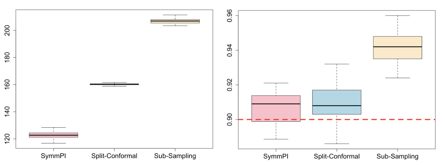
Figure 4: Empirical data example: Prediction set lengths and coverage probabilities for various methods with level $\alpha=0.10$. Left: Prediction set lengths; Right: Empirical coverage probabilities.

6 Conclusion and Discussion

We have presented a general methodology for predictive inference in arbitrary observation models satisfying distributional invariance. We have illustrated that our methods have competitive performance in a two layer hierarchical model. There are a number of intriguing directions for further research. In some examples, the data itself might not satisfy distributional invariance, but some transformation of the data—possibly dependent on unknown parameters—might do so. Can one extend our methods to this setting, possibly leveraging ideas such as joint coverage regions (Dobriban and Lin, 2023)? Moreover, is it possible to learn equivariant maps to enable improved predictive inference, as opposed to designing them as we did in this paper? Studying these questions is expected to benefit the broad applicability of rigorous predictive inference methods.

7 Supplementary Material

Additional notation and definitions. In the supplementary material we will use the following additional notation and definitions. If two sets $A,B$ are in a bijection, we write $A\cong B$. For a group $\mathcal{G}$ acting on a set $\mathcal{Z}$ by an action $\rho$, the stabilizer of an element $z\in\mathcal{Z}$ is the set $\{g\in\mathcal{G}:\rho(g)z=z\}$. The stabilizer is a subgroup of $\mathcal{G}$. For two sets $S,V$, a map $f:S\to V$, and a subset $V^{\prime}\subseteq V$, we denote by $f^{-1}(V^{\prime})$ the preimage of $V^{\prime}$ under $f$.

7.1 Discussion of Equivariance Properties

In this section, we discuss the key properties of deterministic equivariance, distributional equivariance, and distributional invariance, which form the building blocks of our theory. We shed light on the connections between these properties, and on their connections with various classical topics in statistics and the mathematical sciences. These discussions are not strictly needed for understanding the description of our methods.

7.1.1 Deterministic Equivariance

Recall that the deterministic $\mathcal{G}$ equivariance condition (2) requires that for all $z\in\mathcal{Z}$ and all $g\in\mathcal{G}$, $f(\rho(g)z)=\tilde{\rho}(g)f(z)$. Equivalently, one can require that for all $\mathcal{Z}$-valued random variables, $f(\rho(g)Z)=\tilde{\rho}(g)f(Z)$. Given $z\in\mathcal{Z}$, and $\tilde{z}\in\tilde{\mathcal{Z}}$, let $\mathcal{H}_{z},\tilde{\mathcal{H}}_{\tilde{z}}$ be their stabilizers with respect to $\rho,\tilde{\rho}$, respectively. We have the following result:

Proposition 7.1 (Characterizing equivariant maps).

The functions $f$ satisfying the deterministic equivariance condition (2) can be described as follows: partition $\mathcal{Z}$ into orbits, collecting representatives in a set $R$, so that we have the disjoint union $\mathcal{Z}=\cup_{z\in R}O_{z}$. For each orbit representative $z\in R$, choose $f(z)$ such that $\mathcal{H}_{z}$ is a subgroup of $\tilde{\mathcal{H}}_{f(z)}$. For all $z^{\prime}\in O_{z}$, choose any $g\in\mathcal{G}$ such that $z^{\prime}=\rho(g)z$, and define $f(z^{\prime})=\tilde{\rho}(g)f(z)$.

Proof.

First, we show that the procedure from the statement leads to equivariant functions. Indeed, if for some $g^{\prime}\in\mathcal{G}$, $\rho(g)z=\rho(g^{\prime})z$, then the definition of $f$ leads to $f(\rho(g)z)=f(\rho(g^{\prime})z)$, so $\tilde{\rho}(g)f(z)=\tilde{\rho}(g^{\prime})f(z)$. This shows that we must have $g(g^{\prime})^{-1}\in\tilde{\mathcal{H}}_{f(z)}$. Now, $\rho(g)z=\rho(g^{\prime})z$ shows that we have $g(g^{\prime})^{-1}\in\mathcal{H}_{z}$; and since by assumption $\mathcal{H}_{z}$ is a subgroup of $\tilde{\mathcal{H}}_{f(z)}$, the required condition $g(g^{\prime})^{-1}\in\tilde{\mathcal{H}}_{f(z)}$ follows, showing that the above procedure always leads to equivariant functions.

Second, we show that all equivariant functions satisfy these conditions. For any $h\in\mathcal{H}_{z}$, we have $f(z)=f(\rho(h)z)=\tilde{\rho}(h)f(z)$. $\mathcal{H}_{z}\subset\tilde{\mathcal{H}}_{f(z)}$, and since $\mathcal{H}_{z},\tilde{\mathcal{H}}_{f(z)}$ are both subgroups of $\mathcal{G}$, it follows that $\mathcal{H}_{z}$ is a subgroup of $\tilde{\mathcal{H}}_{f(z)}$. Moreover, if $z^{\prime}=\rho(g)z$, by equivariance, we have $f(z^{\prime})=\tilde{\rho}(g)f(z)$; showing that equivariant functions satisfy these conditions. ∎

7.1.2 Distributional Equivariance

We next characterize distributional equivariance. Consider a fixed $z\in\mathcal{Z}$. Recall that for $v\in\mathcal{Z}$, $O_{v}=\{\rho(g)\cdot v:g\in\mathcal{G}\}$ is the orbit of $v$ under $\mathcal{G}$. Denote the distribution of $\rho(G)v$ over the orbit $O_{v}$ with the sigma-algebra generated by the intersection of the sigma-algebra over $\mathcal{Z}$ with $O_{v}$ when $G\sim U$ by $\mu_{v}$. Similarly, for $v\in\tilde{\mathcal{Z}}$, define $\tilde{O}_{v}=\{\tilde{\rho}(g)\cdot v:g\in\mathcal{G}\}$. We have the following result:

Proposition 7.2 (Characterizing distributionally equivariant maps).

The functions $f$ satisfying the distributional equivariance condition (2) can be described as follows: for $P$-almost every $z$, we have that for any measurable set $\tilde{S}\subset\tilde{O}_{f(z)}$ and any $g\in\mathcal{G}$,

$$\mu_{z}(f^{-1}(\tilde{S}))=\mu_{z}(f^{-1}(\tilde{\rho}(g)\tilde{S})).$$ (18)

Informally, this means that the preimages of the elements of the orbit of $f(z)$ under $\mathcal{G}$ have the same density in the original orbit of $z$. Or, “orbits map to orbits, in the natural measure-preserving way”. In comparison, as shown in Section 7.1.1, deterministic $\mathcal{G}$-equivariance requires a more restrictive specific one-to-one correspondence within each orbit.

Proof.

If (1) holds, we can condition on $Z=z$ to deduce that $f(\rho(G)z)=_{d}\tilde{\rho}(G)f(z)$ for $P$-almost every $z$. Now, $f(\rho(G)z)$ is distributed as the pushforward $f\#\mu_{z}$ of $\mu_{z}$ under $f$, while $\tilde{\rho}(G)f(z)\sim\tilde{\mu}_{f(z)}$, so (1) holds iff

$$f\#\mu_{z}=\tilde{\mu}_{f(z)}.$$

By the definition of a pushforward measure, for any measurable set $\tilde{S}\subset\tilde{O}_{\tilde{z}}$, $f\#\mu_{z}(\tilde{S})=\mu_{z}(f^{-1}(\tilde{S})).$ Hence, the above means $\tilde{\mu}_{f(z)}(\tilde{S})=\mu_{z}(f^{-1}(\tilde{S})).$ Since for $G\sim U$, and any $g\in\mathcal{G}$, $\tilde{\rho}(g)\tilde{\rho}(G)f(z)=_{d}\tilde{\rho}(G)f(z)$, it follows that $\tilde{\mu}_{f(z)}(\tilde{\rho}(g)\tilde{S})=\tilde{\mu}_{f(z)}(\tilde{S})$, and thus the above implies that for any $g\in\mathcal{G}$, (18) holds. ∎

For a finite group $\mathcal{G}$, we obtain the following simpler result. Given $z\in\mathcal{Z}$, and $\tilde{z}\in\tilde{\mathcal{Z}}$, let $\mathcal{H}_{z},\tilde{\mathcal{H}}_{\tilde{z}}$ be their stabilizers with respect to $\rho,\tilde{\rho}$, respectively.

Corollary 7.3 (Equivariance in finite groups).

If $\mathcal{G}$ is finite, then given $z\in\mathcal{Z}$ and $\tilde{z}\in\tilde{\mathcal{Z}}$, and the actions $\rho,\tilde{\rho}$ of $\mathcal{G}$ on $\mathcal{Z},\tilde{\mathcal{Z}}$, the existence of an equivariant map $f:O_{z}\to\tilde{O}_{\tilde{z}}$ such that $f(z)=\tilde{z}$ is characterized as follows:

1. Deterministic equivariance is equivalent to $\mathcal{H}_{z}$ being a subgroup of $\tilde{\mathcal{H}}_{\tilde{z}}$, $\mathcal{H}_{z}\leq\tilde{\mathcal{H}}_{\tilde{z}}$.

2. Distributional equivariance is equivalent to the size of the group $\mathcal{H}_{z}$ dividing the size of the group $\tilde{\mathcal{H}}_{\tilde{z}}$, i.e., $|\mathcal{H}_{z}|\mid|\tilde{\mathcal{H}}_{\tilde{z}}|$.

Clearly, the condition for equivariant maps is stricter.

Proof.

The first part follows from Proposition 7.1. For the second part, since $\{\tilde{z}\}\in\tilde{O}_{\tilde{z}}$ is a measurable subset of $\tilde{O}_{\tilde{z}}$, and since for $S\subset O_{v}$ and $G$ distributed uniformly on the finite group $\mathcal{G}$, we have $\mu_{v}(S)=P(\rho(G)v\in S)=|S|/|O_{v}|$, the condition (18) characterizing distributional equivariance becomes that $r(\tilde{z}):=|f^{-1}(\tilde{\rho}(g)\tilde{z})|\in\mathbb{N}_{>0}$ does not depend on $g$. Now, from the orbit-stabilizer theorem (Artin, 2018, Proposition 6.8.4), we have that $\mathcal{G}/\mathcal{H}_{z}\cong O_{z}$, $\mathcal{G}/\tilde{\mathcal{H}}_{z}\cong\tilde{O}_{\tilde{z}}$. Thus, $|\mathcal{G}|/|\mathcal{H}_{z}|=r(\tilde{z})|\mathcal{G}|/|\tilde{\mathcal{H}}_{\tilde{z}}|$, and hence $|\tilde{\mathcal{H}}_{\tilde{z}}|=r(\tilde{z})|\mathcal{H}_{z}|$, and so the size of the group $\mathcal{H}_{z}$ divides the size of the group $\tilde{\mathcal{H}}_{\tilde{z}}$. ∎

As an example for a finite group $\mathcal{G}$, consider any sets of representatives $\mathcal{R},\tilde{\mathcal{R}}$ of the orbits of the action of $\rho$ on $\mathcal{Z}$, and $\tilde{\rho}$ on $\tilde{\mathcal{Z}}$, an arbitary injective map $r:\mathcal{R}\to\tilde{\mathcal{R}}$, and any collection of one-to-one maps $f_{z}:O_{z}\to\tilde{O}_{r(z)}$. Then $f$ defined as $f(z^{\prime})=f_{z}(z^{\prime})$ when $z^{\prime}\in O_{z}$ is distributionally equivariant. For concreteness, let $\mathcal{Z}=\mathcal{Z}^{\prime}=\{0,1,\ldots,j\}$ and $\mathcal{G}=\mathbb{Z}_{j+1}=(\{0,1,\ldots,j\},+)$ acting via addition $g\cdot z=g+z$ modulo $j+1$. Then deterministic equivariance requires $f(g+z)=g+f(z)$ modulo $j+1$, for all $g,z$. This means $f(z+g)=z+f(g)$, so $g+f(z)=z+f(g)$, so with $a=f(0)-0$, we have $f(z)=z+a$ for all $z$. In contrast, distributional equivariance requires that $f(G+z)=_{d}G+f(z)$ modulo $j+1$, when $G\sim U$, and for all $z$. It is clear that any function $f:\mathcal{Z}\to\mathcal{Z}^{\prime}$ satisfies this.

For the special case of the symmetric group where $\mathcal{G}=\mathrm{S}_{n}$, and for the permutation actions $\rho,\tilde{\rho}$ acting on $\mathcal{Z}=\mathcal{Z}_{0}^{n}$, Dean and Verducci (1990) have provided a sufficient condition for a transform $f$ to preserve equivariance. Their condition states that for any $z\in\mathcal{Z}_{0}^{n}$, and any $g^{\prime}\in\mathrm{S}_{n}$, there is $g\in\mathrm{S}_{n}$ such that $g^{\prime}f(z)=f(gz)$. Our result recovers theirs in this special case. Indeed, our condition Corollary 7.2 in this case states that the preimage of the orbit $\{gf(z):g\in S_{n}\}$ under $f$ equals the orbit $\{gz:g\in S_{n}\}$, which matches their condition.

7.1.3 Distributional Invariance

The distributional invariance $Z=_{d}\rho(G)Z$, when $G\sim U$, is equivalent to the distribution of $Z|\{Z\in O_{z}\}$ being $\mu_{z}$, for $P$-almost every $z\in\mathcal{Z}$. Thus, in this case, the orbits (or measurably chosen representatives), are a sufficient statistic for the distribution of $Z$. Thus distributional invariance is an example of conditional ancillarity.

The key advantage of distributional invariance is that it is preserved under compositions. In contrast, this is not always convenient for conditionally ancillarity. Suppose $Z\sim P$, $p\in\mathcal{P}$, is conditionally ancillary given $A$, where $A:\mathcal{Z}\to\mathcal{A}$ is a map, i.e., for almost every $a$ we have that $Z|A=a$ has the same distributions for all $P\in\mathcal{P}$. Now, for a map $f:\mathcal{Z}\to\tilde{\mathcal{Z}}$, we ask when $f(Z)$ is conditionally ancillary given $A$. In general, this is not ensured, because $f$ may map different preimages $A^{-1}(a)$, $a\in\mathcal{A}$ to the same value, and hence the resulting conditional distribution may mix the distributions of $Z|A=a$ with the—possibly $P$-dependent—distributions of $Z$ and $A$.

In contrast, a key advantage of group invariance is that it does not have this restriction. Different orbits may map into the same orbit, and the resulting distribution is still uniform. In the end, this enables the development of broader classes of architectures that preserve invariance and finally power our methods.

7.2 Distribution Shift with Non-symmetric Algorithm

This section is devoted to studying predictive inference in cases where a non-symmetric algorithm is employed, even if we have a distribution shift and so $Z\neq_{d}\rho(G)Z$. We present a novel algorithm along with theoretical coverage guarantees, wherein possibly distinct weights are assigned to various members within a representative set $S$, and the function $f$ may not necessarily be distributionally equivariant.

For a given group $\mathcal{G}$ and a function $\psi(\cdot)$, we consider the induced functions $\mathcal{F}=\{\ell_{g}\mid g\in\mathcal{G}\}$, where each $\ell_{g}$ is defined as $\ell_{g}(\tilde{z})=\psi(\tilde{\rho}(g)\tilde{z})$ for all $\tilde{z}$. Here we focus on a simplified scenario where the set $\mathcal{F}$ is finite and can be represented as $\mathcal{F}=\{\psi_{1},\ldots,\psi_{|\mathcal{F}|}\}$. In this case, in our non-symmetric algorithm, we sample the cosets (or, equivalently, a set of representatives denoted as $S=\{g_{1},\ldots,g_{|\mathcal{F}|}\}$) from a distribution $\Gamma_{S}$ with probabilities given by $(w_{1},\ldots,w_{|\mathcal{F}|})$. The procedure can also be extended to continuous groups using an approach similar to that discussed earlier.

The weights in $\Gamma_{S}$ can be arbitrary but are typically chosen aiming to minimize the coverage gap due to the distribution shift. For example, when considering the group $G=S_{n+1}$ and the function $\psi(z)=z_{n+1}$ for all $z$, the selection of weights is guided by the characteristics of the data structures, such as time series analysis and change point detection (Barber et al., 2023). In these cases, a common strategy is to allocate greater weights to elements that are closer in time to the unobserved data point.

Next, we formally define our prediction set when we do not assign equal weights to the representatives of cosets or we do not have a distributionally equivariant map $f$. We first sample a representative $g$ according to the probability measure $\Gamma_{S}$ and we construct our prediction set as follows:

$$T^{\mathrm{non-sym}}(z_{\mathrm{obs}})=\Bigg{\{}z:\psi(\tilde{\rho}(g)f(\rho^{-1}(g)z))\leqslant Q_{1-\alpha}\bigg{(}\sum_{j=1}^{|\mathcal{F}|}w_{j}\delta_{\psi_{j}(f(\rho^{-1}(g)z))}\bigg{)},\mathrm{obs}(z)=z_{\mathrm{obs}}\Bigg{\}}.$$ (19)

We next provide a coverage property for this prediction set. We let

$$\Delta^{w}:=\sum_{i=1}^{|\mathcal{F}|}w_{i}\mathrm{TV}\big{(}\nu_{i}(f(\rho^{-1}(g_{i})Z)),\nu_{i}(f(Z))\big{)},$$

where $\nu_{i}(x)=\psi_{i}(x)-Q_{1-\alpha}(\sum_{j=1}^{|\mathcal{F}|}w_{j}\delta_{\psi_{j}(x)})$ for all $x$. In addition, we let $F^{w}_{\tilde{z}}$ be the c.d.f. of the random variable $\psi(\rho(g)\tilde{z}),\,g\sim\Gamma_{S}$. Furthermore, we let $F^{w^{\prime}}_{\tilde{z}}$ be the probability it places on individual points, i.e., for $x\in\mathbb{R}$, $F^{w^{\prime}}_{\tilde{z}}(x)=F^{w}_{\tilde{z}}(x)-F^{w-}_{\tilde{z}}(x)$, where $F^{w-}_{\tilde{z}}(x)=\lim_{y\to x,y<x}F^{w}_{\tilde{z}}(y)\geqslant 0$. We then define $t^{w}_{\tilde{z}}:=Q_{1-\alpha}(\sum_{j=1}^{|\mathcal{F}|}w_{j}\delta_{\psi_{j}(\tilde{z})}).$ for all $\tilde{z}$. See Section 8.7 for the proof of the result below.

Theorem 7.4.

Regardless of the weights $(w_{1},\ldots,w_{|\mathcal{F}|})$, and regardless of whether $Z$ is distributionally invariant and $f$ is distributionally equivariant, the prediction set from (19) satisfies the coverage bound

$$-\Delta^{w}\leqslant\bigg{|}P\Big{(}Z\in T^{\mathrm{non-sym}}(Z_{\mathrm{obs}})\Big{)}-(1-\alpha)\bigg{|}\leqslant\mathbb{E}[F^{w^{\prime}}_{f(Z)}(t^{w}_{f(Z)})]+\Delta^{w}.$$

When $Z$ is distributionally invariant over $\mathcal{G}$, the coverage lower bound reduces to $1-\alpha$. If this distributional invariance property does not hold, we see that the prediction set now relies on the set of representatives $S$ that we choose. Therefore, in order to minimize the coverage gap, we suggest choosing each $g_{i}$ from each coset that minimizes the difference between $Z$ and $\rho^{-1}(g_{i})Z$. For the case in Barber et al. (2023), the suggested $g_{i}\in\mathrm{S}_{n+1}$ are permuting the $i$th and the $(n+1)$st entry of $Z$. While it would be desirable to compare the coverage of the symmetric and non-symmetric algorithms, in general, this does not seem straightforward. Therefore, we leave this to future work.

Our coverage conclusion in Theorem 7.4 reduces to the conclusion of non-exchangeable conformal prediction in Theorem 2 and 3 presented in Barber et al. (2023) when we let $\mathcal{G}=\mathrm{S}_{n+1}$ and $\psi(\tilde{z})=e_{n+1}^{\top}\tilde{z}$ and train a non-symmetric non-conformity score in terms of the input order of the data. We present the relevant details as an example, illustrated below:

Example 7.5 (Non-exchangeable conformal prediction).

To recover the results of Barber et al. (2023), we consider $Z=(Z_{1},\ldots,Z_{n+1})^{\top}$, where we have $Z_{i}=(X_{i},Y_{i})$ with $X_{i}$ being the covariate, $Y_{i}$ being the response.

Let $0\leqslant w_{1}\leqslant w_{2}\leqslant\ldots\leqslant w_{n}\leqslant w_{n+1}=1$, and $\tilde{w}_{i}=w_{i}/(\sum_{j=1}^{n+1}w_{j})$, $i\in[n+1]$. Denote by $g_{j}$ the transposition exchanging $j$ and $n+1$, keeping other indices fixed, and note that $g_{j}$, $j\in[n+1]$ is a set of representatives of $\mathcal{G}/\mathcal{H}$. Moreover, $g_{j}z:=z^{(j)}=(z_{1},\ldots$, $z_{j-1},z_{n+1},z_{j+1},\ldots,z_{j})^{\top}$, where we exchange $z_{n+1}\leftrightarrow z_{j}$. We construct the prediction set in the same way as (19) by letting $\psi(x)=e_{n+1}^{\top}x$, $\mathcal{G}=S_{n+1}$, and taking $Z_{i}=(X_{i},Y_{i})$ for all $i\in[n+1]$, and $f(z)=(R(z_{1}),\ldots,R(z_{n+1}))^{\top}$, where $R(z_{i})=|y_{i}-\hat{\mu}^{z}(x_{i})|$, for all $i\in[n+1]$, with $\hat{\mu}^{z}:\mathcal{Z}\to\mathbb{R}$ being non-symmetric in the sense that $\hat{\mu}^{gz}\neq\hat{\mu}^{z}$ for some $g\in\mathrm{S}_{n+1}$. Then, since $\textnormal{TV}\Big{(}\nu_{j}(f(Z)),\nu_{j}(f(g_{j}^{-1}Z))\Big{)}\leqslant\textnormal{TV}\Big{(}f(Z),f(g_{j}^{-1}Z)\Big{)}$ for all $i\in[n+1]$, Theorem 7.4 implies that the coverage probability is lower bounded as

$$P_{Z}\Big{(}Z_{n+1}\in T^{\tilde{w},n+1}(Z_{1:n})\Big{)}\geqslant 1-\alpha-\sum_{j=1}^{n}\tilde{w}_{j}\textnormal{TV}\Big{(}f(g_{j}^{-1}Z),f(Z)\Big{)}.$$

When $f$ is injective and $(Z_{1},\ldots,Z_{n+1})$ has a continuous distribution, Theorem 4.6 implies that

$$P_{Z}\Big{(}Z_{n+1}\in T^{\tilde{w},n+1}(Z_{1:n})\Big{)}\leqslant 1-\alpha+\tilde{w}_{n+1}+\sum_{j=1}^{n}\tilde{w}_{j}\textnormal{TV}\Big{(}f(g_{j}^{-1}Z),f(Z)\Big{)}.$$

Then, these results match with the conclusions in Theorems 2b & 3b of Barber et al. (2023).

Next we discuss the example of a two-layer tree.

Example 7.6 (Non-exchangeable conformal prediction for two-layer trees).

Continuing the example from Section 4.4.1, we consider predicting $Z_{M}^{(K)}$ in the final branch of the two-layer tree depicted in Figure 3, left panel. In the following, we will adopt the notations used there. However, we allow that $g\cdot\Gamma\neq_{d}\Gamma$: for instance, branch growth can be time-ordered and nodes within each branch $\Gamma_{k},k\in[K]$ can have stronger dependence compared to nodes across different branches. In such a scenario, it is appropriate to assign greater weights, denoted as $w_{i}^{(k)},i\in[M],k\in[K]$, to the leaves of the last branch relative to those in earlier branches.

For example, we can pick $0\leqslant w_{1}^{(1)}=\cdots=w_{1}^{(K)}\leqslant\cdots\leqslant w_{M}^{(1)}=\cdots=w_{M}^{(K)}$ and let $\tilde{w}_{i}^{(k)}=w_{i}^{(k)}/(\sum_{j=1,k=1}^{M,K}w_{j}^{(k)}).$ We let $g_{s}^{(q)},s\in[K],q\in[M]$ be the set of representatives of $\mathcal{G}/\mathcal{H},$ and $g_{s}^{(q)}z:=z^{(s,q)}=(R,\Gamma_{1},\cdots,\Gamma_{q-1},\Gamma_{K}^{s},\Gamma_{q+1},\cdots,\Gamma_{K-1},\Gamma_{q}),$ where

$$\Gamma_{K}^{s}=(C_{K},Z_{1}^{(K)},\cdots,Z_{s-1}^{(K)},Z_{M}^{(K)},Z_{s+1}^{(K)},\cdots,Z_{s}^{(K)}).$$

Here we first exchange the $q$-th branch with the $K$-th branch and then permute the last entry of the current $q$-th branch (the original $K$-th branch) with its $s$-th entry. We keep $f(z)=|z|$ for all $z\in\mathcal{Z}$, as we did in Section 4.4.1. Therefore, Theorem 7.4 implies that the coverage probability is lower bounded as

$$P_{Z}\Big{(}Z_{M}^{(K)}\in T^{\tilde{w}}(Z_{i}^{(k)},i\in[M],k\in[K]\setminus(M,K))\Big{)}\geqslant 1-\alpha-\sum_{i=1,k=1}^{M,K\setminus(M,K)}\tilde{w}_{i}^{(k)}\textnormal{TV}\Big{(}|(g_{i}^{(k)})^{-1}Z|,|Z|\Big{)}.$$

When $Z=(R,\Gamma_{1},\cdots,\Gamma_{K})$ has a continuous distribution, Theorem 4.6 implies that

$$P_{Z}\Big{(}Z_{M}^{(K)}\in T^{\tilde{w}}(Z_{i}^{(k)},i\in[M],k\in[K]\setminus(M,K))\Big{)}$$

$$\leqslant 1-\alpha+\tilde{w}_{M}^{(K)}+\sum_{i=1,k=1}^{M,K\setminus(M,K)}\tilde{w}_{i}^{(k)}\textnormal{TV}\Big{(}|\big{(}g_{i}^{(k)}\big{)}^{-1}Z|,|Z|\Big{)}.$$

7.3 Coarsening Approach for Predictive Inference on Graphs

From a practical perspective, if the graph is large, we can coarsen it. For instance, we can use a hierarchical graph clustering method to cluster nodes. We keep edges between the clustered nodes with associated multiplicities; thus we obtain a graph with multiple edges allowed between nodes. The automorphism group of the new graph can then be viewed as a subgroup of the original graph that fixes the vertices within each clustered node.

We can apply our method to the clustered graph by considering the values of clusters for which node observations are missing as also missing. This construction leads to prediction sets at the cluster-level, which we can view as prediction sets for any symmetric function of the node values, such as for their sum. If there is only one missing observation per cluster, then we can back out prediction sets for the individual nodes; e.g., if using the sum to aggregate, by subtracting the sum of the labeled nodes in the cluster. If there are several nodes with missing values in a cluster, then we obtain a prediction set for their sum.

For the tree-structured graphical model from Section 4.4.1 we can predict at a cluster after coarsening the graph as follows. We can define the clusters as the branches $C_{k},Z_{1}^{(k)},\ldots,Z_{M}^{(k)}$, for $k\in[K]$. We can re-write the data as $\Gamma=(R,\Gamma_{1}^{\top},\ldots,\Gamma_{K}^{\top})^{\top}$, where we treat every branch $\Gamma_{k}:=(C_{K},Z_{1}^{(K)},\ldots,Z_{M}^{(K)})^{\top},k\in[K]$ as one component. Our goal is to predict the sum of values of the last branch. We let $\psi(z)=|(0,0_{(K-1)\cdot(M+1)}^{\top},1_{M+1}^{\top})^{\top}z|$, so the quantile is $t^{(2)}_{z}:=Q_{1-\alpha}(|1^{\top}\gamma_{1}|,\ldots,|1^{\top}\gamma_{K}|)$, where $\gamma_{k}$ are the realized values of $\Gamma_{k}$, $k\in[K]$, and the prediction set is given by

$$T^{\mathrm{SymmPI}}(z_{\mathrm{obs}})=\{z:|1^{\top}\gamma_{K}|\leqslant t^{(2)}_{\tilde{z}},\,\mathrm{obs}(z)=z_{\mathrm{obs}}\}.$$

7.4 Graph Neural Network Construction for Un-supervised Learning

Here we give two graph neural network constructions for un-supervised learning: a simpler one that is easier to understand, and a more sophisticated one that has bettter performance by interpolating with standard conformal prediction.

7.4.1 GNN for Unsupervised Learning

We design a fixed GNN architecture where the neighborhood structure of the graph is as in Figure 3:

1. We let the sample means over the second-layer nodes be proxy statistics, setting

   $$\tilde{P}^{(k,0)}={M}^{-1}\sum_{i=1}^{M}Z_{i}^{(k)},\,k=1,\ldots,K.$$

   More generally, any permutation invariant functions over $Z_{i}^{(k)},i\in[M]$ are a valid choice. We also set the proxy $\tilde{P}^{0}$ for the root note to be zero, and let $Z_{i}^{(k,0)}=Z_{i}^{(k)}$.

2. We apply a modified two-layer MPGNN. In the first layer, we have the following.

   1. We update the leaves as $Z_{i}^{(k,1)}=|Z_{i}^{(k,0)}-\tilde{P}^{(k,0)}|$.

   2. We update the proxy variables as $\tilde{P}^{(k,1)}=\sum_{i\in\mathcal{N}(k)}\bigl{(}\tilde{P}^{(k,0)}-Z_{i}^{(k,0)}\bigr{)}^{2}/(M-1),$ which corresponds to (3) with $f_{0}(x)=y$, $f_{11}(x,y)=(x-y)^{2}/(M-1)$ and $f_{12}(\tilde{P}^{(k,0)},\tilde{P}^{0})=0$.

   In the second layer of the MPGNN, we update the leaves as follows:

   $$Z_{i}^{(k,2)}=\frac{Z_{i}^{(k,1)}}{\sqrt{\tilde{P}^{(k,1)}}}=\frac{\left|Z_{i}^{(k)}-{\sum_{i=1}^{M}Z_{i}^{(k)}}/{M}\right|}{\sqrt{\frac{1}{M-1}\sum_{j\in\mathcal{N}(k)}\biggl{(}Z_{j}^{(k)}-\frac{\sum_{j=1}^{M}Z_{j}^{(k)}}{M}\biggr{)}^{2}}}.$$

   This corresponds to (3) with $f_{1}(x,y)=x/\sqrt{y},f_{0}(x,y)=y$,

3. We construct prediction sets for $Z_{M}^{K}$ by following the method in Section 4.1.

7.4.2 Interpolation with Conformal Inference

Here, for every variable we have two channels.

1. Step 0: (Initialization)

   1. We let $\bar{Z}=\frac{1}{KM}\sum_{k=1}^{K}\sum_{i=1}^{M}Z_{i}^{(k,0)}$ and $\hat{\sigma}$ the sample standard deviation of the full sample. We set the zeroth-layer node $\tilde{P}^{0}$ to be $(\bar{Z},\hat{\sigma})^{\top}$.

   2. For first-layer nodes $\tilde{P}^{(k,0)}$, we initialize them as $(\frac{1}{M}\sum_{i=1}^{M}Z_{i}^{(k,0)},\hat{\sigma}_{k})^{\top}$, where $\hat{\sigma}_{k}$ is the standard error of the $\{Z_{i}^{(k,0)}\}_{i=1}^{M}.$

   3. For leaves, we augment all features $Z_{i}^{(k,0)}$ with a constant $1$; as the second channel is not used and only kept so that all nodes have two features. We denote $X_{i}^{(k,0)}=(Z_{i}^{(k,0)},1)^{\top}.$

2. Step 1: (Update)

   We update $\tilde{P}^{(k,0)}$ to $\tilde{P}^{(k,1)}$ for all $k\in[K]$ via $\tilde{P}^{(k,0)}$ and $\tilde{P}^{0}$ as

   $$\tilde{P}^{(k,1)}=f^{(1)}(\tilde{P}^{(k,0)},\tilde{P}^{0}) =\bigg{(}\bigg{|}\frac{\tilde{P}^{(k,0)}(1)-\tilde{P}^{0}(1)}{\tilde{P}^{(k,0)}(2)/\sqrt{M}}\bigg{|},\tilde{P}^{(k,0)}(2)\bigg{)}^{\top}=\bigg{(}\bigg{|}\frac{\bar{Z}_{k}-\bar{Z}}{\hat{\sigma}_{k}/\sqrt{M}}\bigg{|},\hat{\sigma}_{k}\bigg{)}^{\top}.$$

   We keep other variables—the zeroth layer node $\tilde{P}^{(1)}$ and leaves $X_{i}^{(k,1)},\forall k\in[K],i\in[M]$—unchanged: $\tilde{P}^{(1)}=\tilde{P}^{(0)}$ and $X_{i}^{(k,1)}=X_{i}^{(k,0)},\forall k\in[K],i\in[M]$.

3. Step 2: (Update)

   Again, we only update $\tilde{P}^{(k,1)}$, via

   $$\tilde{P}^{(k,2)}=f^{(2)}_{0}\bigg{(}\tilde{P}^{(k,1)},\sum_{i=1}^{M}f^{(2)}_{11}(\tilde{P}^{(k,1)},X_{i}^{(k,1)})+f^{(2)}_{12}(\tilde{P}^{(k,1)},\tilde{P}^{(1)})\bigg{)}.$$

   Here we take $f^{(2)}_{11}(\tilde{P}^{(k,1)},X_{i}^{(k,1)})=Z_{i}^{(k,1)}\mathbb{K}(\tilde{P}^{(k,1)}(1))/M$, for some kernel $\mathbb{K}$. Therefore, $\sum_{i=1}^{M}f^{(2)}_{11}(\tilde{P}^{(k,1)},X_{i}^{(k,1)})$ $=\bar{Z}_{k}\mathbb{K}(\tilde{P}^{(k,1)}(1)).$ We set $\mathbb{K}(x)=I(|x|\leqslant c)$ with some constant $c$, so that

   $$\sum_{i=1}^{M}f_{11}^{(2)}(\tilde{P}^{(k,1)},X_{i}^{(k,1)})=\bar{Z}_{k}I\bigg{(}\bigg{|}\frac{\bar{Z}_{k}-\bar{Z}}{\hat{\sigma}_{k}/\sqrt{M}}\bigg{|}\leqslant c\bigg{)}.$$

   For $f_{12}^{(2)}$ we let $f_{12}^{(2)}(\tilde{P}^{(k,1)},\tilde{P}^{(1)})=\bar{Z}(1-\mathbb{K}(\tilde{P}^{(k,1)}(1)))=\bar{Z}I\bigg{(}\bigg{|}\frac{\bar{Z}_{k}-\bar{Z}}{\hat{\sigma}_{k}/\sqrt{M}}\bigg{|}>c\bigg{)}$ Therefore,

   $$\tilde{P}^{(k,2)}=\Bigg{(}\bar{Z}_{k}I\bigg{(}\bigg{|}\frac{\bar{Z}_{k}-\bar{Z}}{\hat{\sigma}_{k}/\sqrt{M}}\bigg{|}\leqslant c\bigg{)}+\bar{Z}I\bigg{(}\bigg{|}\frac{\bar{Z}_{k}-\bar{Z}}{\hat{\sigma}_{k}/\sqrt{M}}\bigg{|}>c\bigg{)},\hat{\sigma}_{k}\Bigg{)}.$$ (20)

   We keep $X_{i}^{(k,2)}=X_{i}^{(k,1)}$ and $\tilde{P}^{(2)}=\tilde{P}^{(1)}.$

4. Step 3: (Update)

   We finally update all $X_{i}^{(k,3)}$, for all $i\in[M],k\in[K]$. We let

   $$X_{i}^{(k,3)} =f_{0}^{(3)}(X_{i}^{(k,2)},f_{1}^{(3)}(X_{i}^{(k,2)},\tilde{P}^{(k,2)}))$$

   $$=\Bigg{(}\Bigg{|}Z_{i}^{(k)}-\left[\bar{Z}I\left(\frac{|\bar{Z}_{k}-\bar{Z}|}{\hat{\sigma}_{k}/\sqrt{M}}\leqslant c\right)+\bar{Z}_{k}I\left(\frac{|\bar{Z}_{k}-\bar{Z}|}{\hat{\sigma}_{k}/\sqrt{M}}>c\right)\right]\bigg{|}/\hat{\sigma}_{k},1\Bigg{)}^{\top}.$$

   We take $v=(v_{1};\ldots;v_{n+1})^{\top}\in\mathbb{R}^{2\cdot(n+1)}$ and let $v_{n+1}=(1,0)^{\top}.$

7.5 Simulation with Random Sample Sizes

In this simulation, we let the number of branches be $K=20$. For every branch, we let $N_{k}\sim\mathrm{Unif}(\{10,20\}),k\in[K]$ independently in the setting of unsupervised learning. The other settings are the same as for the fixed sample size regime presented in the main text. The final statistics are:

$$\Bigg{|}Z_{i}^{(k)}-\left[\bar{Z}I\left(\frac{|\bar{Z}_{k}-\bar{Z}|}{\hat{\sigma}_{k}/\sqrt{M}}\leqslant c\right)+\bar{Z}_{k}I\left(\frac{|\bar{Z}_{k}-\bar{Z}|}{\hat{\sigma}_{k}/\sqrt{M}}>c\right)\right]\bigg{|}/\hat{\sigma}_{k},$$

for $i\in[M],k\in[K]$, where $\bar{Z}=\frac{1}{K}\sum_{k=1}^{K}\frac{1}{N_{k}}\sum_{i=1}^{N_{k}}Z_{i}^{(k)}$, for unsupervised learning.

For supervised learning, we also consider a setting very similar to the fixed sample size regime presented in the main text. The only difference is that we sample $N_{k}\sim\mathrm{Unif}(\{20,40\}),k\in[K]$ independently for each branch and use the first half of all branches as the training data. The output statistics are the same as (15) for supervised learning except that the datapoints used for training $\hat{\mu}_{k}(\cdot),k\in[K]$ and $\hat{\mu}(\cdot)$ are of random sizes.

In addition to the methods used in the main text, we also compare with hierarchical conformal prediction (HCP) (Lee et al., 2023). The results are presented in Tables 3 and 4, respectively. The conclusions are identical to those from the experiments from the main text. Here HCP performs well, similarly to our method. However, of course our method is more general and applicable to any symmetry group, not just to the hierarchical setting, as described in the main text.

	Estimator	$\sigma^{2}=10$	$\sigma^{2}=2$	$\sigma^{2}=0.5$	$\sigma^{2}=0$
$\alpha=0.05$	Length: SymmPI	2.076 (0.012)	2.097 (0.016)	2.138 (0.224)	2.019 (0.012)
	Coverage: SymmPI	0.957 (0.022)	0.950 (0.023)	0.949 (0.023)	0.952 (0.022)
	Length: HCP	41.076 (0.865)	8.064 (0.142)	2.774 (0.030)	1.996 (0.010)
	Coverage: HCP	0.948 (0.027)	0.955 (0.017)	0.945 (0.022)	0.952 (0.024)
	Length: Conformal	38.222 (0.716)	7.859 (0.138)	2.740 (0.031)	1.977 (0.009)
	Coverage: Conformal	0.945 (0.025)	0.950 (0.019)	0.943 (0.023)	0.947 (0.025)
	Length: Subsampling	44.377 (0.958)	9.149 (0.168)	3.129 (0.067)	2.220 (0.048)
	Coverage: Subsampling	0.949 (0.026)	0.954 (0.017)	0.949 (0.021)	0.951 (0.025)
	Length: Single-Tree	Inf	Inf	Inf	Inf
	Coverage: Single-Tree	1.0 (0.0)	1.0 (0.0)	1.0 (0.0)	1.0 (0.0)
$\alpha=0.15$	Length: SymmPI	1.516 (0.010)	1.524 (0.014)	1.547 (0.014)	1.470 (0.012)
	Coverage: SymmPI	0.844 (0.033)	0.842 (0.038)	0.850 (0.033)	0.857 (0.039)
	Length: HCP	28.771 (0.612)	5.835 (0.127)	2.030 (0.017)	1.451 (0.008)
	Coverage: HCP	0.849 (0.039)	0.837 (0.030)	0.848 (0.032)	0.853 (0.040)
	Length: Conformal	28.006 (0.668)	5.798 (0.125)	2.016 (0.016)	1.450 (0.007)
	Coverage: Conformal	0.846 (0.041)	0.837 (0.033)	0.843 (0.030)	0.853 (0.038)
	Length: Subsampling	30.821 (0.670)	6.347 (0.148)	2.172 (0.042)	1.549 (0.028)
	Coverage: Subsampling	0.848 (0.039)	0.838 (0.031)	0.848 (0.034)	0.863 (0.035)
	Length: Single-Tree	1.758 (0.052)	1.770 (0.053)	1.749 (0.056)	1.738 (0.047)
	Coverage: Single-Tree	0.872 (0.031)	0.877 (0.031)	0.874 (0.031)	0.878 (0.031)

Table 3: Prediction set length and coverage probability of our method and three benchmarks for unsupervised learning with a random sample size; same protocol as in Table 1.

	Estimator	$\sigma^{2}=10$	$\sigma^{2}=2$	$\sigma^{2}=0.5$	$\sigma^{2}=0$
$\alpha=0.05$	Length: SymmPI	2.080 (0.021)	2.105 (0.024)	2.067 (0.012)	2.013 (0.016)
	Coverage: SymmPI	0.955 (0.021)	0.942 (0.024)	0.950 (0.020)	0.951 (0.019)
	Length: HCP	12.618 (0.023)	3.098 (0.037)	2.071 (0.013)	1.993 (0.015)
	Coverage: HCP	0.953 (0.023)	0.952 (0.024)	0.948 (0.023)	0.950 (0.019)
	Length: Conformal	12.353 (0.248)	3.051 (0.038)	2.051 (0.012)	1.976 (0.014)
	Coverage: Conformal	0.948 (0.024)	0.948 (0.025)	0.945 (0.023)	0.948 (0.020)
	Length: Subsampling	12.821 (0.618)	3.152 (0.091)	2.069 (0.058)	1.990 (0.051)
	Coverage: Subsampling	0.923 (0.025)	0.919 (0.032)	0.927 (0.028)	0.932 (0.022)
	Length: Single-Tree	Inf	Inf	Inf	Inf
	Coverage: Single-Tree	1.0 (0.0)	1.0 (0.0)	1.0 (0.0)	1.0 (0.0)
$\alpha=0.15$	Length: SymmPI	1.512 (0.008)	1.531 (0.009)	1.507 (0.008)	1.463 (0.008)
	Coverage: SymmPI	0.854 (0.037)	0.847 (0.038)	0.857 (0.033)	0.852 (0.034)
	Length: HCP	7.986 (0.153)	2.143 (0.024)	1.510 (0.008)	1.451 (0.008)
	Coverage: HCP	0.855 (0.032)	0.857 (0.031)	0.858 (0.034)	0.854 (0.036)
	Length: Conformal	7.890 (0.163)	2.125 (0.025)	1.500 (0.008)	1.444 (0.008)
	Coverage: Conformal	0.848 (0.033)	0.853 (0.033)	0.855 (0.033)	0.851 (0.037)
	Length: Subsampling	8.414 (0.293)	2.229 (0.054)	1.565 (0.035)	1.479 (0.032)
	Coverage: Subsampling	0.841 (0.037)	0.843 (0.035)	0.846 (0.038)	0.836 (0.035)
	Length: Single-Tree	1.732 (0.046)	1.745 (0.051)	1.727 (0.043)	1.689 (0.050)
	Coverage: Single-Tree	0.876 (0.031)	0.878 (0.026)	0.881 (0.028)	0.867 (0.038)

Table 4: Prediction set length and coverage probability of our method and three benchmarks for supervised learning with a random sample size; same protocol as in Table 1.

7.6 Additional Information about Empirical Data Example

7.6.1 Discusson of Modelling Assumptions

Finally, we discuss modelling assumptions, and in particular the applicability of exchangeability assumptions to the empirical dataset. The covariate $X_{1}$ is the number of days lacking sleep. Within a branch, this covariate has a time trend, taking values $0,1,\ldots,9$. Thus, its values for one datapoint are not exchangeable with the values for other data points within the same branch. However, even if the covariates are not exchangeable, the values $\varepsilon_{k}=(\varepsilon_{1}^{(k)},\ldots,\varepsilon_{9}^{(k)})^{\top}$ of the random noise can be assumed exchangeable. Therefore, when we fit $\hat{\mu}_{k},k\in[18]$ accurately, the residuals (or non-conformity scores) are “nearly” exchangeable. This is expected to be a sufficient assumption for analyzing this dataset. In fact, when $\varepsilon_{i}^{(k)}$ is independent of $X_{i}^{(k)}$, some distributions of $\varepsilon_{i}^{(k)}$ (such as the Gaussian distribution) admit an upper bound $TV(Y_{i}^{(k)}-\hat{\mu}_{k}(X_{i}^{(k)}),Y_{i}^{(k)}-\mu_{k}^{*}(X_{i}^{(k)}))\leqslant C\mathbb{E}_{X_{i}^{(k)}}[|\hat{\mu}_{k}(X_{i}^{(k)})-\mu_{k}^{*}(X_{i}^{(k)}))|]$. Hence, if we estimate $\mu_{k}^{*}$ accurately, then the empirical residuals $Y_{i}^{(k)}-\hat{\mu}_{k}(X_{i}^{(k)})$ will be approximately exchangeable.

We remark that Dunn et al. (2022) also make a similar exchangeability assumption. However, they train a common $\hat{\mu}(\cdot)$ for all branches. For a given $k\in[18]$, the residuals $|Y_{i}^{(k)}-\hat{\mu}(X_{i}^{(k)})|,i\in[9]$ may not necessarily be exchangeable, since $\hat{\mu}(\cdot)$ could be very different from $\mu_{k}^{*}(\cdot)$ and thus these residuals can be strongly affected by $X_{i}^{(k)}$.

7.6.2 Additional Empirical Data Plots

In this section, we present the additional plots on the length of prediction sets and coverage probability via various methods with level $\alpha=0.20$ in the following figure 5.

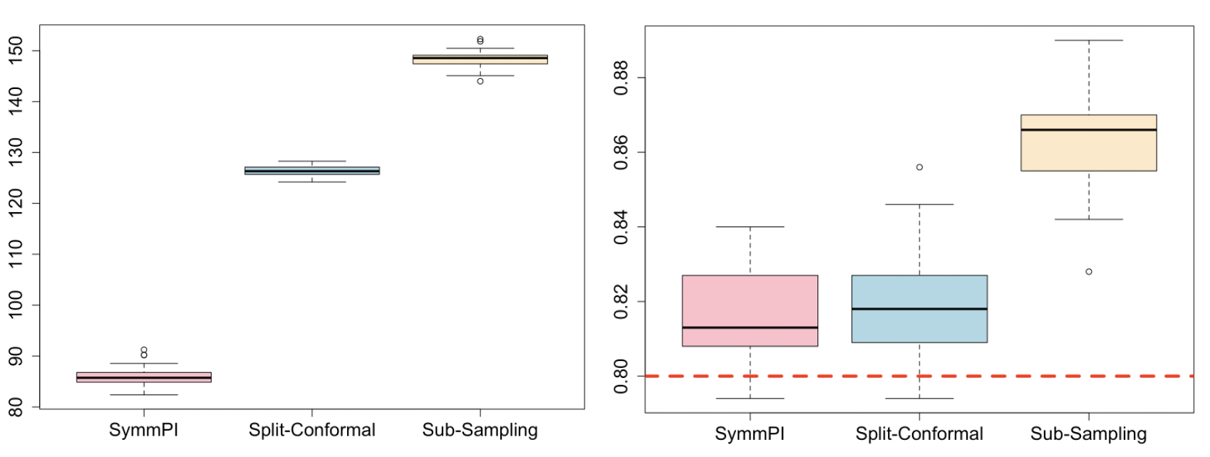
Figure 5: Prediction set lengths and coverage probabilities for various methods with level $\alpha=0.20$. Left: Prediction set lengths; Right: Empirical coverage probabilities.

8 Proofs

8.1 Proof of Theorem 4.2

Proof.

Since $\mathrm{obs}(z)=z_{\mathrm{obs}}$ by definition,

$$P(Z\in T_{r}(Z_{\mathrm{obs}})) =P(\psi(f(Z))<t_{f(Z)}\textnormal{ or }\psi(f(Z))=t_{f(Z)},\,V<\delta_{f(Z)}).$$ (21)

Now, for all $\tilde{z}\in\tilde{\mathcal{Z}}$, by the definitions of $t$ from (4) and $\delta$ from (6), we have

$$P_{G}(\psi(\tilde{\rho}(G)\tilde{z})<t_{\tilde{z}}\textnormal{ or }\psi(\tilde{\rho}(G)\tilde{z})=t_{\tilde{z}},\,V<\delta_{\tilde{z}})=F^{-}_{\tilde{z}}(t_{\tilde{z}})+F^{\prime}_{\tilde{z}}(t_{\tilde{z}})\delta_{\tilde{z}}=1-\alpha.$$

Hence, letting $\tilde{z}=f(z)$, we have for all $z\in\mathcal{Z}$ that $P_{G}(\psi(\tilde{\rho}(G)f(z))<t_{f(z)}\textnormal{ or }\psi(\tilde{\rho}(G)f(z))=t_{f(z)},\,V<\delta_{f(z)})=1-\alpha$. Therefore, using that $Z$ is $\mathcal{G}$-distributionally-invariant and $t$ is $\mathcal{G}$-invariant, (21) equals

$$P_{G,Z}(\psi(\tilde{\rho}(G)f(Z))<t_{\tilde{\rho}(G)f(Z)}\textnormal{ or }\psi(\tilde{\rho}(G)f(Z))=t_{\tilde{\rho}(G)f(Z)},\,V<\delta_{\tilde{\rho}(G)f(Z)})$$

$$=P_{G,Z}(\psi(\tilde{\rho}(G)f(Z))<t_{f(Z)}\textnormal{ or }\psi(\tilde{\rho}(G)f(Z))=t_{f(Z)},\,V<\delta_{f(Z)})$$

$$=\mathbb{E}_{Z}[P_{G}(\psi(\tilde{\rho}(G)f(Z))<t_{f(Z)}\textnormal{ or }\psi(\tilde{\rho}(G)f(Z))=t_{f(Z)},\,V<\delta_{f(Z)}))]=1-\alpha.$$

This proves the first relation in (8). The second relation follows since $T_{r}(z_{\mathrm{obs}})\subset T^{\mathrm{SymmPI}}(z_{\mathrm{obs}})$. Next, for $\tilde{z}\in\tilde{\mathcal{Z}}$, by the definitions of $t$ from (4) and of $F^{\prime}$,

$$P_{G}(\psi(\tilde{\rho}(G)\tilde{z})\leqslant t_{\tilde{z}})=F_{\tilde{z}}(t_{\tilde{z}})\leqslant 1-\alpha+F^{\prime}_{\tilde{z}}(t_{\tilde{z}}).$$

Hence, as above

$$P(Z\in T^{\mathrm{SymmPI}}(Z_{\mathrm{obs}})) =P(\psi(f(Z))\leqslant t_{f(Z)},\,\mathrm{obs}(Z)=z_{\mathrm{obs}})=P(\psi(f(Z))\leqslant t_{f(Z)})$$ (22)

$$=\mathbb{E}_{Z}[P_{G}(\psi(\tilde{\rho}(G)f(Z))\leqslant t_{f(Z)})]\leqslant 1-\alpha+\mathbb{E}_{Z}[F^{\prime}_{f(Z)}(t_{f(Z)})],$$

proving the third relation in (8).

∎

8.2 Proof of Proposition 4.3

Let $\mathcal{F}_{\tilde{z}}=\{\psi(\tilde{\rho}(g)\tilde{z}),\,g\in\mathcal{G}\}$ be the set of values of $\psi(\tilde{\rho}(g)\tilde{z})$, $g\in\mathcal{G}$. If $\mathcal{H}_{\tilde{z}}$ is a subgroup of $\mathcal{G}$, clearly for any $c\in\mathcal{F}_{\tilde{z}}$, there is a unique coset $\mathcal{C}=\mathcal{H}_{\tilde{z}}\cdot g$, for some $g\in\mathcal{G}$, such that for all $g^{\prime}\in\mathcal{C}$, $\psi(\tilde{\rho}(g^{\prime})\tilde{z})=c$. Thus, the size of each coset is $|\mathcal{H}_{\tilde{z}}|$. Thus, $F^{\prime}_{\tilde{z}}(x)\leqslant|\mathcal{H}_{\tilde{z}}|/|\mathcal{G}|$ for all $x\in\mathbb{R}$, which implies that $P(Z\in T^{\mathrm{SymmPI}}(Z_{\mathrm{obs}}))\leqslant 1-\alpha+\mathbb{E}|\mathcal{H}_{f(Z)}|/|\mathcal{G}|.$ Moreover, if $\mathcal{H}_{\tilde{z}^{\prime}}$ does not depend on $\tilde{z}^{\prime}$, then, $\mathcal{H}$ is clearly a group. In this case, $F^{\prime}_{f(Z)}(x)\leqslant|\mathcal{H}|/|\mathcal{G}|$ for all $x\in\mathbb{R}$, almost surely for $Z\sim P$; and hence $P(Z\in T^{\mathrm{SymmPI}}(Z_{\mathrm{obs}}))\leqslant 1-\alpha+|\mathcal{H}|/|\mathcal{G}|.$

8.3 Proof of Proposition 4.7

The proof of Proposition 4.7 is derived using the same method as outlined in Theorem 4.2 of Dobriban and Lin (2023). Therefore, we omit the details.

8.4 Proof of Theorem 4.6

Proof.

By (22), we have

$$P_{Z}\Big{(}Z\in T^{\mathrm{SymmPI}}(Z_{\mathrm{obs}})\Big{)}=\bigg{\{}P_{Z}\Big{(}\psi(f(Z))\leqslant t_{f(Z)}\Big{)}-P_{G,Z}\Big{(}\psi(\tilde{\rho}(G)f(Z))\leqslant t_{f(Z)}\Big{)}\bigg{\}}$$

$$+P_{G,Z}\Big{(}\psi(\tilde{\rho}(G)f(Z))\leqslant t_{f(Z)}\Big{)}=\mathbf{(i)}+\mathbf{(ii)}.$$

For the first term, by definition,

$$|\mathbf{(i)}| =\Bigg{|}\int_{G}\int_{Z}\bigg{[}I\Big{(}\psi(f(Z))\leqslant t_{f(Z)}\Big{)}-I\Big{(}\psi(\tilde{\rho}(G)f(Z))\leqslant t_{f(Z)}\Big{)}\bigg{]}dP(Z)dP(G)\Bigg{|}$$

$$=\Bigg{|}\int_{Z}\mathbb{E}_{G^{\prime}\sim U(\mathcal{G}/\mathcal{H})}\bigg{[}I\Big{(}\psi(f(Z))\leqslant t_{f(Z)}\Big{)}-I\Big{(}\psi(\tilde{\rho}(G^{\prime})f(Z))\leqslant t_{f(Z)}\Big{)}\bigg{]}dP(Z)\Bigg{|}\leqslant\Delta.$$

In the last line, we have used that $I\Big{(}\psi(f(z))\leqslant t_{f(z)}\Big{)}=I(\nu(\tilde{z})\leqslant 0)$ and $I\Big{(}\psi(\tilde{\rho}(G^{\prime})f(z))\leqslant t_{f(z)}\Big{)}=I(\nu(\tilde{\rho}(G^{\prime})\tilde{z})\leqslant 0)$; which also uses that $t$ is $\mathcal{G}$-invariant.

For the second term, by the definition of $t_{\tilde{z}}$ from (4), we have $\mathbf{(ii)}\leqslant\alpha.$ Combining the upper bounds on $\mathbf{(i)}$ and $\mathbf{(ii)}$, we obtain the lower bound in (11). Next, following the same proof procedure as in Theorem 4.2, for term $\mathbf{(ii)}$, we obtain that

$$P_{G,Z}\Big{(}\psi(\tilde{\rho}(G)f(Z))\leqslant t_{f(Z)}\Big{)}\leqslant 1-\alpha+\mathbb{E}[F^{\prime}_{f(Z)}(t_{f(Z)})].$$

Combining this with the upper bound of $\mathbf{(i)}$, the upper bound in (11) follows. ∎

8.5 Proof of Propositions 5.3 and 5.4

The proof of Propositions 5.3 and 5.4 follows directly from our construction of the deterministic equivariant massage-passing graph neural network and the distributional invariance of the input variable $Z$. Therefore, we omit the details.

8.6 Proof of Theorem 5.5

Proof.

Due to the data-generating process and the definition of $t_{\tilde{z}}$ in (16), for the given $\vec{n}=(n_{1},\ldots,n_{K})^{\top}$, it holds that $t_{\tilde{z}}=t_{g_{\vec{n}}\tilde{z}}$, for any $g_{\vec{n}}\in\mathcal{G}_{\vec{n}}=\mathrm{S}_{n_{1}}\otimes\mathrm{S}_{n_{2}}\otimes\ldots\otimes\mathrm{S}_{n_{K}}$. According the definition of $\mathcal{G}_{\vec{n}}$, and $t_{(\cdot)}$, recalling $\psi_{\vec{n}}(\tilde{z})=\tilde{z}_{n_{K}}^{(K)}$ for all $\tilde{z}\in\tilde{\mathcal{Z}}$, it holds conditionally on $\vec{n}$ that

$$P_{Z}\Big{(}\psi_{\vec{n}}(f(Z))>t_{f(Z)}\Big{)}=P_{G_{\vec{n}},Z}\Big{(}\psi_{\vec{n}}(G_{\vec{n}}\cdot f(Z))>t_{f(Z)}\Big{)}$$

$$\qquad=\mathbb{E}_{Z}\mathbb{E}_{G_{\vec{n}}}\Big{[}I\Big{(}\psi_{\vec{n}}(G_{\vec{n}}\cdot f(Z))>t_{f(Z)}\Big{)}\Big{]}=\mathbb{E}_{Z}\bigg{[}\frac{1}{n_{K}}\sum_{j=1}^{n_{K}}I([f(Z)]_{j}^{(K)}>t_{f(Z)})\bigg{]}.$$

We next define $\tilde{\psi}(x)=e_{K}^{\top}x$, where $e_{K}\in\mathbb{R}^{K}$ with the $K$-th entry being unity and others being zero, for all $x\in\mathbb{R}^{K}$. Furthermore, for the given $n$, we let $h:\mathcal{Z}^{*}\rightarrow\in\mathbb{R}^{K}$ by defining its $m$-th output entry as $[h(Z_{1},\ldots,Z_{K})]_{m}=\frac{1}{n_{m}}\sum_{j=1}^{n_{m}}I(f(Z_{j}^{(m)})>t_{f(Z)}),m\in[K]$.

Next, we take the randomness of $Z,\vec{N}$ into consideration. By the exchangeability of $(Z_{1},\ldots,Z_{K})^{\top}$ and the definition of $t_{(\cdot)}$, it holds that $h(Z_{1},\ldots,Z_{K})$ $=_{d}G^{\prime}h(Z_{1},\ldots,Z_{K})$ for $G^{\prime}\sim\mathrm{Unif}(\mathrm{S}_{K})$. Therefore, according to the definition of $\tilde{\psi}$ and $h(\cdot)$, it holds that

$$\mathbb{E}_{Z}\bigg{[}\frac{1}{N_{K}}\sum_{j=1}^{N_{K}}I([f(Z)]_{j}^{(K)}>t_{f(Z)})\bigg{]} =\mathbb{E}_{Z}\bigg{[}\tilde{\psi}(h(Z))\bigg{]}=\mathbb{E}_{Z,G^{\prime}}\bigg{[}\tilde{\psi}(G^{\prime}\cdot h(Z))\bigg{]}$$

$$=\mathbb{E}_{Z}\bigg{[}\frac{1}{K}\sum_{k=1}^{K}\frac{1}{N_{k}}\sum_{j=1}^{N_{k}}I([f(Z)]_{j}^{(k)}>t_{f(Z)})\bigg{]}\leqslant\alpha.$$

Therefore, we obtain

$$P\Big{(}Z\in T^{\mathrm{SymmPI}}(Z_{\mathrm{obs}},\vec{N})\Big{)} =P_{N,Z}(\psi_{\vec{N}}(f(Z))\leqslant t_{f(Z)},\,\mathrm{obs}(Z)=Z_{\mathrm{obs}})\geqslant 1-\alpha.$$

The upper bound can be proved in a similar way as the corresponding upper bound in the proof of Theorem 4.2, and we omit the details. ∎

8.7 Proof of Theorem 7.4

By the definition of the prediction set in (19), we have

$$P\bigg{(}\psi(\tilde{\rho}(G)f(\rho^{-1}(G)Z)>Q_{1-\alpha}\Big{(}\sum_{j=1}^{|\mathcal{F}|}w_{j}\delta_{\psi_{j}(f(\rho^{-1}(G)Z))}\Big{)}\bigg{)}$$

$$\qquad=\sum_{i=1}^{|\mathcal{F}|}w_{i}P\bigg{(}\psi(\tilde{\rho}(G)f(\rho^{-1}(G)Z)>Q_{1-\alpha}\Big{(}\sum_{j=1}^{|\mathcal{F}|}w_{j}\delta_{\psi_{j}(f(\rho^{-1}(G)Z))}\Big{)}\Big{|}G=g_{i}\bigg{)}.$$

Since $G$ is independent of $Z$, we obtain

$$\sum_{i=1}^{|\mathcal{F}|}w_{i}P\bigg{(}\psi(\rho(G)f(\rho^{-1}(G)Z)>Q_{1-\alpha}\Big{(}\sum_{j=1}^{|\mathcal{F}|}w_{j}\delta_{\psi_{j}(f(\rho^{-1}(G)Z))}\Big{)}\Big{|}G=g_{i}\bigg{)}$$

$$\qquad=\sum_{i=1}^{|\mathcal{F}|}w_{i}P\bigg{(}\psi_{i}(f(\rho^{-1}(g_{i})Z)>Q_{1-\alpha}\Big{(}\sum_{j=1}^{|\mathcal{F}|}w_{j}\delta_{\psi_{j}(f(\rho^{-1}(g_{i})Z))}\Big{)}\bigg{)}$$

$$\qquad\leqslant\sum_{i=1}^{|\mathcal{F}|}w_{i}P\bigg{(}\psi_{i}(f(Z))>Q_{1-\alpha}\Big{(}\sum_{j=1}^{|\mathcal{F}|}w_{j}\delta_{\psi_{j}(f(Z))}\Big{)}\bigg{)}+\sum_{i=1}^{|\mathcal{F}|}w_{i}\mathrm{TV}\big{(}\nu_{i}(f(\rho^{-1}(g_{i})Z)),\nu_{i}(f(Z))\big{)},$$

where $\nu_{i}(x)=\psi_{i}(x)-Q_{1-\alpha}(\sum_{j=1}^{|\mathcal{F}|}w_{j}\delta_{\psi_{j}(x)}).$ The inequality above holds since we can write

$$P\bigg{(}\psi_{i}(f(Z))>Q_{1-\alpha}\Big{(}\sum_{j=1}^{|\mathcal{F}|}w_{j}\delta_{\psi_{j}(f(Z))}\Big{)}\bigg{)}=I\big{(}\nu_{i}(f(Z))>0\big{)}$$

and

$$I\bigg{(}\psi_{i}(f(\rho^{-1}(g_{i})Z)>Q_{1-\alpha}\Big{(}\sum_{j=1}^{|\mathcal{F}|}w_{j}\delta_{\psi_{j}(f(\rho^{-1}(g_{i})Z))}\Big{)}\bigg{)}=I\big{(}\nu_{i}(f(\rho^{-1}(g_{i})Z))>0\big{)}.$$

Subsequently, we prove upper and lower bounds for term

$$\sum_{i=1}^{|\mathcal{F}|}w_{i}P\bigg{(}\psi_{i}(f(Z))>Q_{1-\alpha}\Big{(}\sum_{j=1}^{|\mathcal{F}|}w_{j}\delta_{\psi_{j}(f(Z))}\Big{)}\bigg{)}.$$

For the upper bound, this term is at most $\alpha$ by definition. For the lower bound, following an argument similar to the proof of Theorem 4.2, we obtain

$$\sum_{i=1}^{|\mathcal{F}|}w_{i}P\bigg{(}\psi_{i}(f(Z))\leqslant Q_{1-\alpha}\Big{(}\sum_{j=1}^{|\mathcal{F}|}w_{j}\delta_{\psi_{j}(f(Z))}\Big{)}\bigg{)}\leqslant 1-\alpha+\mathbb{E}_{Z}[F^{w^{\prime}}_{f(Z)}(t^{w}_{f(Z)})].$$

We then conclude the proof.

References

- Anderson and Robinson (2001) M. J. Anderson and J. Robinson. Permutation tests for linear models. Australian & New Zealand Journal of Statistics, 43(1):75–88, 2001.
- Angelopoulos et al. (2023) A. N. Angelopoulos, S. Bates, et al. Conformal prediction: A gentle introduction. Foundations and Trends® in Machine Learning, 16(4):494–591, 2023.
- Artin (2018) M. Artin. Algebra. Pearson, 2018.
- Babai (2016) L. Babai. Graph isomorphism in quasipolynomial time. In Proceedings of the forty-eighth annual ACM symposium on Theory of Computing, pages 684–697, 2016.
- Balkin et al. (2000) T. Balkin, D. Thome, H. Sing, M. Thomas, D. Redmond, N. Wesensten, J. Williams, S. Hall, G. Belenky, et al. Effects of sleep schedules on commercial motor vehicle driver performance. Technical report, United States. Department of Transportation. Federal Motor Carrier Safety Safety Administration, 2000.
- Barber et al. (2023) R. F. Barber, E. J. Candes, A. Ramdas, and R. J. Tibshirani. Conformal prediction beyond exchangeability. The Annals of Statistics, 51(2):816–845, 2023.
- Bates et al. (2021) S. Bates, A. Angelopoulos, L. Lei, J. Malik, and M. Jordan. Distribution-free, risk-controlling prediction sets. Journal of the ACM (JACM), 68(6):1–34, 2021.
- Bates et al. (2023) S. Bates, E. Candès, L. Lei, Y. Romano, and M. Sesia. Testing for outliers with conformal p-values. The Annals of Statistics, 51(1):149–178, 2023.
- Belenky et al. (2003) G. Belenky, N. J. Wesensten, D. R. Thorne, M. L. Thomas, H. C. Sing, D. P. Redmond, M. B. Russo, and T. J. Balkin. Patterns of performance degradation and restoration during sleep restriction and subsequent recovery: A sleep dose-response study. Journal of sleep research, 12(1):1–12, 2003.
- Blum-Smith and Villar (2022) B. Blum-Smith and S. Villar. Equivariant maps from invariant functions. arXiv preprint arXiv:2209.14991, 2022.
- Candès et al. (2023) E. Candès, L. Lei, and Z. Ren. Conformalized survival analysis. Journal of the Royal Statistical Society Series B: Statistical Methodology, 85(1):24–45, 2023.
- Chatzipantazis et al. (2023) E. Chatzipantazis, S. Pertigkiozoglou, K. Daniilidis, and E. Dobriban. Learning augmentation distributions using transformed risk minimization. Transactions on Machine Learning Research, 2023. URL https://openreview.net/forum?id=LRYtNj8Xw0.
- Chen et al. (2020) S. Chen, E. Dobriban, and J. H. Lee. A group-theoretic framework for data augmentation. Journal of Machine Learning Research, 21(245):1–71, 2020.