Information engine with feedback delay based on a two level system
Abstract
An information engine based on a two level system in contact with a thermal reservoir is studied analytically. The model incorporates delay time between the measurement of the state of the system and the feedback. The engine efficiency and work extracted per cycle are studied as a function of delay time and energy spacing between the two levels. It is found that the range of delay time over which one can extract work from the information engine increases with temperature. For delay times comparable to the relaxation time, efficiency and work per cycle are both maximum when , the energy difference between the levels. Generalized Jarzynski equality and the generalized integral fluctuation theorem are explicitly verified for the model. The results from the model are compared with the simulation results for a feedback engine based on a particle moving in a square potential. The variation of efficiency, work per cycle and efficacy with the delay time is compared using relaxation time in the two state model as the fitting parameter and leads to good fit.
I Introduction
An information engine uses the information gained from a measurement of the system to
extract work from thermal fluctuations [1, 2]. Historically it
was Maxwell who first suggested a thought experiment involving a demon whose measurements of molecular velocities
can be used to transfer heat from a cold to a hot body thus violating the second law of
thermodynamics. It is now generally accepted that there is no violation of the second law if
one considers the entropy generation associated with erasure of memory involved in
the measurement process [3, 4, 2, 5, 6].
For alternative views, see the following references [7, 8, 9, 10, 11]. Recently information engine or Maxwell’s demon, as it
is usually referred to, has been implemented experimentally in a variety of systems both classical
[12, 13, 14, 15] and quantum
[16, 17, 18, 19, 20, 21].
Stochastic thermodynamics deals with study of thermodynamics of small systems where fluctuations dominate [22]. Several fluctuation theorems have offered valuable insights into the production of entropy and the statistical connections between work and free energy for systems operating significantly beyond equilibrium [23, 24, 25, 26]. These results in stochastic thermodynamics has been generalized to the cases when there is measurement and feedback during the process [27, 28]. For example, the Jarzynski relation which connects the fluctuations in work, , during a non-equilibrium process to the free energy difference, , between the final and initial equilibrium states [25] has been modified to a form,
| (1) |
where is the inverse temperature and the angular brackets represent average over multiple trajectories of
the system starting from the equilibrium distribution.
This relation, known as the Generalized Jarzynski Relation (GJR), is valid for non-equilibrium processes
incorporating feedback mechanism. The right hand side of GJR, (referred to as efficacy), is the
sum of the probabilities of observing the time reversed trajectories in the time reversed protocols for
all possible protocols. is a measure of the reversibility of the process. The largest value that
can take is the number of outcomes in the measurement process and is attained for a fully reversible process.
In the absence of feedback, and the GJR reduces to the usual Jarzynski relation [25].
The experimental verification of GJR has been done for few systems [12, 29, 30, 31]. In the case of processes involving precise measurements (error-free) and
feedback mechanisms, we can establish a Generalized Integral Fluctuation Theorem (GIFT) expressed as
. Here, represents the information acquired
during the measurement process, and is the unavailable information to be determined through
the time-reversed process [32].
In the context of an information engine, efficiency quantifies the degree of conversion of information to work.
High efficiency requires a slow process thus compromises on power. Thus it is important to tune the
engine parameters such that efficiency and power are as required. Many recent works
have investigated methods to enhance the efficiency and power of information engine, both in experiments
[14, 33, 34] and in theoretical studies
[35, 36, 37]. Information engines based on colloidal
particle moving through a harmonic potential [38, 39, 15]
as well as periodic potentials [12, 40] have been studied.
These studies look into the possibility of extracting work or converting the information about
the position of the particle into work with the help of a feedback scheme. An information engine based
on a two level system where the state of the system is measured and feedback is effected has been theoretically
studied [41]. These simple information engine systems offer ways to understand the optimisation schemes.
In this study, we perform an analytical investigation of a two-state information engine that is in
contact with a heat bath. The model is similar to the one studied by Jaegon et al [41] but differs
in that in the current model there is a feedback delay between the measurement and feedback. The analytical
results are derived by assuming that the cycle time of the engine is large compared to the relaxation time of the system.
The feedback time and the energy difference between the two states
are the two parameters with respect to which the efficiency and work per cycle of the engine are studied.
We compare the analytical findings with the numerical results
obtained from the simulation of a particle moving within a one-dimensional periodic square potential. Over-damped
Langevin dynamics is used to simulate the motion of the particle.
Further, the generalized fluctuation relations of stochastic thermodynamics for this system are verified.
The paper is structured as follows: The model for the information engine is introduced in the next section and the assumptions and parameters of the model are defined. In Sec. III, we start with the study of information engine without feedback delay (Sec. III.1) and then generalize to one that incorporates feedback delay time (Sec. III.2). The engine performance parameters are worked out and the fluctuation theorems are verified. Sec. III.3 provides a comparison between the analytical results and the results obtained from the simulation of the particle moving in periodic square potential. Finally, in Sec. IV, we offer a summary of our findings and engage in a discussion of the results.
II The Model
The information engine consists of a two level system in contact with a thermal reservoir at temperature . The energies of the higher energy state (up state) and the lower energy state (down state) of the system are and respectively. Also present as a part of the information engine is an observer (Maxwell’s demon) who measures the state of the system at regular intervals of time, ( is an integer), and implements a feedback process depending on the outcome of the measurement. The feedback process is as follows: If the system is measured to be in the up state in the measurement, the demon flips the state of the system to down state at a time , with . is the feedback delay time. If the system is measured to be in the down state, no feedback is initiated.
The master equation for the process is given by
| (2) |
where and are the probabilities for finding the system in up and down states respectively and and are the rates of transition between the states (see Fig. 1).

Detailed balance condition in equilibrium dictates that , where . We shall work in energy unit where . The relaxation time for the process is, . Note that for the case when the measurement outcome is up state, the master equation has to be integrated in two time segments: from to and then from to . This is because, if the the measurement gives up state as the outcome, the state will be flipped after a delay time of .
III Results and analysis
In the analysis that follows, we shall assume that the time between the state flip and the next measurement time, , is much larger than the relaxation time . This would imply that the system is in equilibrium at the beginning of each cycle. We first work out the simpler case when (immediate feedback with no delay time). Subsequently, we relax this constraint and work out the results for the more general case.
III.1 Feedback engine with no delay time ()
We consider here the case when the feedback is implemented right after the measurement. The probability for spotting the particle in the up state during the measurement is,
| (3) |
which is the equilibrium distribution. Average information gathered during the measurement is,
| (4) |
This is related to the cost of running the information engine. Processing this information requires a minimum of of energy, associated with resetting the memory bits involved in the measurement process.
III.1.1 Efficiency and work per cycle
Since a work of is extracted every time the particle is spotted in the up state, the average work extracted per cycle is,
| (5) |
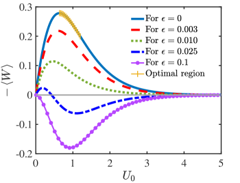
The variation of average work per cycle (WPC) as a function of is shown in Fig. 2 (blue solid curve). The optimal value for at which WPC is a maximum is . The fact that has to be of the order of for optimal work extraction can be understood as follows: If is much smaller than , the chance of spotting the system in the up state will be close to , but the resultant work extraction per flip will be small. For much larger than , the probability of observing the system in the up state reduces drastically leading again to low value of WPC.
The efficiency, defined as the ratio of work extracted to the cost of running the engine, is given by
| (6) |
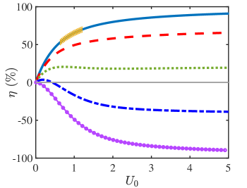
The efficiency is a monotonically increasing function of and saturates for values of as seen in Fig. 3 (blue solid curve). In the limit of , . It is easily seen that in this limit, . But this maximal efficiency happens at the expense of WPC going to zero. At the value of at which WPC is a maximum, . For optimal choices that do not compromise either efficiency or work per cycle, should lie between and (the shaded yellow region in the blue solid curve in Figs. 2 and 3) for the case when .
III.1.2 Verifying generalized Jarzynski relation
We compute the right and left hand sides of the GJR (Eq. (1)) separately for verifying the relation. Note that for the system considered because the energy spacing remains the same after the feedback process. The work variable, , can take two values: (i) , when particle is observed in the up state and (ii) , when the particle is observed in the down state. The corresponding probabilities are, and . Thus the left hand side of the GJR is
| (7) | |||||
The right hand side of GJR is , where and are probabilities to be determined by running the two protocols backwards for the case when the particle was observed in the up state in the forward cycle and in the down state in the forward cycle respectively. Note that the time reversed protocols start with the system in the equilibrium state and no feedback is involved. is the probability of finding the particle in the up state at time with the state flipped at (Note that the flip would in general be carried out at , but we are looking at an engine with ). is thus the probability of finding the system in the down state in equilibrium, which is . is the probability of finding the particle in the down state at time , starting from equilibrium with no flip in the state. Thus is also given by . Thus the right hand side of GJR is given by,
| (8) |
Comparing Eqs. (7) and (8) we see that GJR is valid for this system.
Efficacy, , is a measure of how reversible the engine is. In the limit , and . This is the largest possible value for for feedback process which involves two measurement outcomes. When , and efficacy becomes, . For this case there is no feedback because the two states are identical and the flip does not make a difference to the state. As expected, the GJR reduces to the usual Jarzynsky equality for this case. When , efficacy becomes . The information is used in least optimal manner in this situation. This is because the demon, rather than extracting work, flips the state when the system is in the lower of the energy states. Note that with , the up state becomes the lower energy state.
III.1.3 Verifying generalized integral fluctuation theorem
To verify GIFT, we need the values of the information variable, and the unavailable information, for the two outcomes of the measurement. For the case when the system is measured in the up state, is given by and for the other case information is, . The unavailable information for the two cases are given by and respectively. Using the values of the probabilities determined above for the occurrence of the two outcomes, we have,
| (9) | |||||
and thus verifying GIFT for this case. Note that if one ignores the unavailable information, , then GIFT will be found to be violated. This is because we have assumed a measurement without error. In fact, one can easily see that , giving a value less than one.
III.2 Feedback engine with delay time ()
We now consider the case where there is a finite feedback delay time, , between the measurement and state flip. As discussed above, the relaxation time for the system is . Delay in implementing the feedback would imply that at the instant of a state flip, there is a finite probability that the system’s state differs from the measured state. These probabilities are:
where we have defined as the probability that the state of the system is at time given that its state at time is ().
III.2.1 Efficiency and work per cycle
The average work extracted per cycle can be computed by taking into consideration the above probabilities. The average work extracted per cycle is
| (10) |
where . The first term in the above equation accounts for the positive work extraction that happens when the state of the system is measured in the up state and it is also in the up state at the time of the state flip. The second term corresponds to the negative work extracted, that happens when the state is measured to be up but has switched to down state during the delay time, .
In Fig. 2 we have shown the variation of WPC with for different finite delay times: (red dashed curve), (green dotted curve), (blue dash-dotted curve) and (connected circles). The value of is taken to be for all the cases. As expected WPC is reduced for larger delay times because the information gained is utilised less optimally with increasing delay time. Also observed is the shift in the location of the peak value of WPC to smaller as delay time is increased. This means that for a fixed value of , the maximum of WPC occurs for larger temperatures as delay time is increased. For large delay times compared to , WPC becomes negative (connected circle curve for in Fig. 2) indicating that most of the times when the state is flipped, it is in the down state. At intermediate delay times, the WPC takes both positive and negative values with the WPC values initially increasing from zero and then becoming negative and eventually approach zero from below (see dash-dotted curve for in Fig. 2).
The efficiency of the information engine with feedback delay is given by,
| (11) |
The average information, is the same as that given in the previous section. This is because the feedback delay time has no bearing on the measurement probability when the cycle time is large compared to the relaxation time and the feedback delay time. Fig. 3 shows the variation of efficiency as a function of for the same set of values for considered above for the case of WPC. Relaxation time, , is also the same. We have seen that for , the efficiency increases monotonically with , attaining the maximum value of as tends to infinity. But as the delay time is increased, the peak in efficiency shifts to lower values of . As expected, the peak value of efficiency also decreases as is increased. For of the order of , both efficiency and WPC are maximum for . These features are seen in the green dotted curve () and the blue dash-dotted curve () in Figs. 2 and 3.
III.2.2 Generalized Jarzynski relation with feedback delay
We have seen in the previous section that without feedback delay, the efficacy, . It was shown that this was indeed equal to thus verifying GJR. We now find for the case with non-zero delay time and propose to verify the validity of GJR for this case.
For the present case, in the expression for , is the probability of finding the system in the up state at with the system starting from equilibrium at and a flip of the state being carried out at (Note that there is no measurement involved in the reverse process.). Thus is given by the sum of two terms: (i) the probability that at the time just before the flip, the system is in the down state (which means after the flip, the system will be in the up state) and then it remains in the up state till time and (ii) the probability that at the time just before the flip, the system is in the up state (which means after the flip, the system will be in the down state) and then to be found in the up state at the time . on the other hand is just the probability of the system to be found in the down state in equilibrium. This is the reverse process when the particle in measured in the down state in the forward process and does not involve any feedback. Thus we have,
| (12) |
This gives,
| (13) |
which reduces to for the case when , as expected.
To evaluate the LHS of GJR, note that the possible values of are , and , with probabilities , and . Therefore,
| (14) |
Substituting for and making use of the relation , the above expression reduces to
| (15) |
which is the same as (Eq. 13), thus validating the GJR. One can similarly verify the validity of GIFT, which is presented in the appendix A.
III.3 Comparison with simulation results
Consider a particle moving in one dimension in a periodic square potential
| (16) | |||||
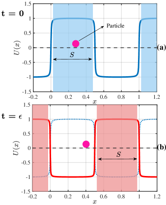
with as shown in Fig. 4. The particle is in contact with a heat bath at temperature, . One can implement an information engine using this system by measuring the position of the particle and initiating a feedback protocol [40]. The protocol closely resembles that of the two state information engine discussed above and is as follows: At times given by , a measurement of the particle’s position is carried out. If the particle is located in the region with higher potential energy, referred to as region (see Fig. 4 (a)), then the potential is flipped (that is, ) at a time where is the engine cycle time and is the feedback delay time. If the particle is not spotted in , then no feedback process is initiated. The interval is kept large enough to ensure that the system equilibriates before each measurement. This is not a necessary part of the current model but is done so that the comparison with the analytical results from the two sate model can be made.
Even though the state space of the current system, which is a continuum of states, is different from that of the two level system considered above, there are similarities. In equilibrium, the probability for finding the particle in the region of higher potential will be equal to the probability of finding the two level system in the up state. In the two-state model, the relaxation to equilibrium is governed by a single relaxation time. However, this process might differ for the particle in the square potential and could involve multiple time scales whose values depend on the height and the period of the potential. But as a first approximation, one can model the relaxation using a single relaxation time approximation. This would allow us to compare the simulation results for the particle in the square potential with the analytical results for the two level system by using the relaxation time as a fit parameter. We carry out this comparison below.
The simulation has been carried out using the over-damped Langevin equation,
| (17) |
where is the mass of the particle and is the friction coefficient. is the thermal noise with zero average and the correlation function is given by . Fluctuation-dissipation relation connects the strength of the noise, , to the friction coefficient, , by the relation: . is the conservative force arising from a potential, . The square potential is modelled using the function . The value of the parameter determines the sharpness of the potential and the parameter is adjusted so as to make the amplitude of the potential to be . Fig. 4 shows the shape of , for and which gives a good approximation to with .
The above equation Eq. (17) has been integrated numerically using the discretized version [42],
| (18) |
where is the time step and is a Gaussian distributed random variable with zero mean and variance equal to . Since does not have a discontinuity at , one needs to choose the region appropriately. We have chosen region such that it approximately covers the elevated part of the potential (see Fig. 4). is taken as the region between and to before the flip (Fig. 4 (a)) and from to after the flip (Fig. 4 (b)), encompassing a total length of and periodically repeating. We work with a system of units defined by , and . Time scale in the problem is set by , which is set to . The length scale of the problem is the period of the potential, which is . The integration time step of the simulation is taken to be . The time step has been kept small because at the region where the potential changes, close to , the forces can be very large. We have verified the convergence of the solution by checking out sample trajectories at one order smaller time step. Simulations have been carried out by varying the amplitude of the potential as well as the delay time . The WPC, efficiency and efficacy are computed by averaging over cycles. The averaging over large number of trials are particularly necessary for finding efficacy accurately [43, 44].
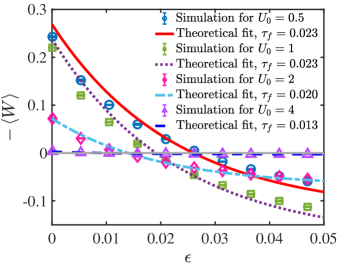
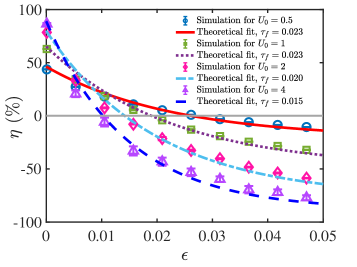
Work per cycle as a function of the delay time for various values of are shown in Fig. 5. As expected, for a given value of , WPC decreases with because the particle might drift away from the higher potential region if one waits longer for the feedback process after the measurement. It is observed that the zero crossing of WPC occurs at lower values of for larger values. This implies that the range of delay time over which the information engine can extract work decreases with decreasing temperature. For small , the WPC reduces by a factor of almost when is varied from to , which is approximately half the relaxation time (see red solid line in Fig. 5). This drop is more drastic for higher values of with WPC dropping by nearly one fourth its value at (see blue dash-dot line in Fig. 5). The curves in Fig. 5 are theoretical fit to the data obtained using the analytic results from the two state model. The relaxation time, , is the fit parameter. We see that there is good fit for all values of considered. This justifies the single relaxation time approximation. It is seen that value of depends on with decreasing as increases. The dependency of efficiency on is given in Fig. 6 for different values of . Like in the case of WPC the efficiency decreases monotonically with delay time. The theoretical fits using the two state results yield similar values of as those obtained from the WPC curve fits.
Efficacy, , has been computed by finding the average from the simulations. The dependency of on the delay time for various values of are shown in Fig. 7. The plot qualitatively resembles those found in the experimentally realized information engine based on a particle moving in a sinusoidal potential [12]. The maximum value that efficacy can take is for this feedback engine as there are two outcomes possible during the measurement. High efficacy values are obtained for small delay times and large . For and , we find efficacy values close to . As expected, the efficacy approaches one as the delay time is increased implying that the Jarzynski equality holds when the feedback is redundant. The theoretical fit for this case leads to values of close to those obtained from the previous fits.
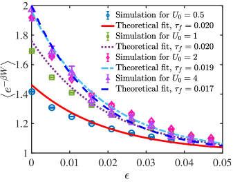
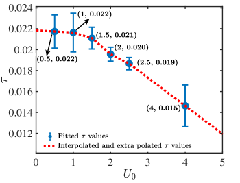
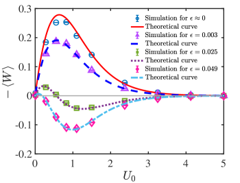
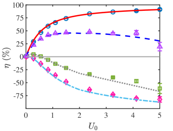
We have averaged the values of obtained from the three sets of fittings carried out above. This gives the variation of as a function of and is shown in Fig. 8. Further, we extrapolate this data to get estimates of for arbitrary values of close to the ones used in the simulations. It is seen that the relaxation time has a strong dependence on the amplitude of the potential, particularly for large values of . We have used the extrapolated data of values to plot the theoretical curves for WPC vs. and vs. along with the results obtained from simulation. These results are shown in Figs. 9 and 10 respectively. There is excellent match between simulation data and model results. Note that the plots of WPC vs. and vs. in Figs. 2 and 3 respectively are for fixed value, whereas for the present case varies with . It is seen from vs plot (Fig. 10) that for short delay times compared to the relaxation time the efficiency increases with (red solid curve). But at larger delay times the efficiency is maximum at intermediate values of (blue dashed curve and black dotted curve).
IV Conclusion
Information engine based on a two state model is possibly the simplest information
engine that can be studied with feedback delay time incorporated. The model allows for
an exact calculation of important engine performance indicators: efficiency, work extracted per cycle
and efficacy. The key control parameters of the engine are the feedback delay time and the energy gap
between the levels or alternately the temperature at which the engine functions. Some of the important
observations from the analytical study of the two state system with feedback are the following:
(i) The engine performance deteriorates with increasing delay time. As delay time becomes large
compared to the relaxation time, one would expect the work extracted
per cycle to saturate to a negative value. This is because the system is more likely to be in
the down state () at the time of the state flip. The efficacy in this
limit will saturate to value , indicating that the information gained is not utilized in
extracting work from the thermal fluctuations.
(ii) For the case of zero delay time the efficiency increases monotonically with whereas
WPC has a peak at intermediate . For finite delay time the peak in WPC and shift to lower
values of .
(iii) The range of delay time over which the engine can extract positive work increase as
decreases, or equivalently the range increases with temperature.
(iv) For delay time of the order of the relaxation time, both WPC and have maxima close to
but below (in units of ). Since is the level spacing, this implies that for a
fixed level spacing the optimal temperature to run the engine is roughly given by is of the same
order as the energy difference between the levels.
The information engine presented here allowed for verification of generalized fluctuation theorems of stochastic thermodynamics. The importance of the unavailable information term in the GIFT relation is explicitly brought out. It is to be noted that the introduction of error into the measurement process will alter the form of the GIFT. In that scenario, the in the LHS of the GIFT will not be present. In the context of stochastic thermodynamics of feedback systems, this simple model can also be of pedagogic interest to understand various fluctuation theorems.
Comparison of the model results with simulation of an information engine based on a particle moving in square potential leads to good match. The efficacy variation as a function of delay time shows the same features that were observed in the experimentally realized information engine based on a particle moving in a sinusoidal potential [12]. The fit values of the relaxation time determined from variation of efficiency, WPC and efficacy with , all give similar values of for all values of considered. The variation of WPC and efficiency with for the particle based information engine has similar features as that for the two state system. The details of the behavior are however different due to the dependence of relaxation time on the amplitude of the square potential.
The current work assumes that the cycle time is large compared to the relaxation time, so that one can assume equilibrium conditions at the beginning of each cycle. This is the reason one had to look at WPC, rather than power of the engine. One can extend the analysis to the case where cycle time is finite. One then needs to work out the steady state probability with feedback in place. Another improvement to the model could be introduction of error in the measurement process. This would make the model more realistic and will allow one to optimize the engine in the presence of imperfect measurements. Work is in progress to incorporate these modifications to the model. Most of the results discussed here should be experimentally accessible in the framework of colloidal particle based information engines.
Acknowledgements.
TJ would like to acknowledge financial support under the DST-SERB Grant No: CRG/2020/003646.Appendix A Generalized integral fluctuation theorem (GIFT) with feedback delay
To show that GIFT holds, we need to prove . The possible values of are , and , with probabilities , and respectively. The corresponding values of are , and respectively. And the values for are , and respectively (where and are given by Eq. (12)).
| (19) | |||||
Substituting for and simplifying,
| (20) | |||||
Substituting for and and making use of the relation and , the above expression reduces to
| (21) | |||||
where .
Simplifying 21 we get,
| (22) |
References
- Clerk Maxwell [1871] J. Clerk Maxwell, Theory of Heat (Longmans, Green, and Co., London, UK, 1871).
- Maruyama et al. [2009] K. Maruyama, F. Nori, and V. Vedral, Rev. Mod. Phys. 81, 1 (2009).
- Landauer [1961] R. Landauer, IBM J. Res. Dev. 5, 183 (1961).
- Bennett [1982] C. H. Bennett, International Journal of Theoretical Physics 21, 905 (1982).
- Sagawa and Ueda [2009] T. Sagawa and M. Ueda, Physical review letters 102, 250602 (2009).
- Leff and Rex [2003] H. S. Leff and A. F. Rex, Computing 2 (2003).
- Earman and Norton [1998] J. Earman and J. D. Norton, Studies In History and Philosophy of Science Part B: Studies In History and Philosophy of Modern Physics 29, 435 (1998).
- Earman and Norton [1999] J. Earman and J. D. Norton, Studies In History and Philosophy of Science Part B: Studies In History and Philosophy of Modern Physics 30, 1 (1999).
- Hemmo and Shenker [2010] M. Hemmo and O. Shenker, The Journal of Philosophy 107, 389 (2010).
- Norton [2011] J. D. Norton, Studies in History and Philosophy of Science Part B: Studies in History and Philosophy of Modern Physics 42, 184 (2011).
- Kish and Granqvist [2012] L. B. Kish and C. G. Granqvist, EPL (Europhysics Letters) 98, 68001 (2012).
- Toyabe et al. [2010] S. Toyabe, T. Sagawa, M. Ueda, E. Muneyuki, and M. Sano, Nature physics 6, 988 (2010).
- Bérut et al. [2012] A. Bérut, A. Arakelyan, A. Petrosyan, S. Ciliberto, R. Dillenschneider, and E. Lutz, Nature 483, 187 (2012).
- Saha et al. [2021] T. K. Saha, J. N. Lucero, J. Ehrich, D. A. Sivak, and J. Bechhoefer, Proceedings of the National Academy of Sciences 118 (2021).
- Paneru et al. [2018a] G. Paneru, D. Y. Lee, T. Tlusty, and H. K. Pak, Physical review letters 120, 020601 (2018a).
- Koski et al. [2014a] J. V. Koski, V. F. Maisi, J. P. Pekola, and D. V. Averin, Proceedings of the National Academy of Sciences 111, 13786 (2014a).
- Najera-Santos et al. [2020] B.-L. Najera-Santos, P. A. Camati, V. Métillon, M. Brune, J.-M. Raimond, A. Auffèves, and I. Dotsenko, Phys. Rev. Research 2, 032025(R) (2020).
- Averin et al. [2011] D. V. Averin, M. Möttönen, and J. P. Pekola, Physical Review B 84, 245448 (2011).
- Camati et al. [2016] P. A. Camati, J. P. Peterson, T. B. Batalhão, K. Micadei, A. M. Souza, R. S. Sarthour, I. S. Oliveira, and R. M. Serra, Physical review letters 117, 240502 (2016).
- Naghiloo et al. [2018] M. Naghiloo, J. Alonso, A. Romito, E. Lutz, and K. Murch, Physical review letters 121, 030604 (2018).
- Chida et al. [2017] K. Chida, S. Desai, K. Nishiguchi, and A. Fujiwara, Nature communications 8, 1 (2017).
- Jarzynski [2013] C. Jarzynski, Prog. Math. Phys. 63, 145 (2013).
- Evans et al. [1993] D. J. Evans, E. G. D. Cohen, and G. P. Morriss, Physical review letters 71, 2401 (1993).
- Gallavotti and Cohen [1995] G. Gallavotti and E. G. D. Cohen, Physical review letters 74, 2694 (1995).
- Jarzynski [1997] C. Jarzynski, Phys. Rev. Lett. 78, 2690 (1997).
- Crooks [1999] G. E. Crooks, Physical Review E 60, 2721 (1999).
- Parrondo et al. [2015] J. M. Parrondo, J. M. Horowitz, and T. Sagawa, Nat. Phys. 11, 131 (2015).
- Sagawa and Ueda [2010] T. Sagawa and M. Ueda, Physical review letters 104, 090602 (2010).
- Koski et al. [2014b] J. V. Koski, V. F. Maisi, T. Sagawa, and J. P. Pekola, Phys. Rev. Lett. 113, 030601 (2014b).
- Paneru et al. [2020] G. Paneru, S. Dutta, T. Sagawa, T. Tlusty, and H. K. Pak, Nature Communications 11, 1012 (2020).
- Paneru and Kyu Pak [2020] G. Paneru and H. Kyu Pak, Advances in Physics: X 5, 1823880 (2020).
- Ashida et al. [2014] Y. Ashida, K. Funo, Y. Murashita, and M. Ueda, Physical Review E 90, 052125 (2014).
- Paneru et al. [2018b] G. Paneru, D. Y. Lee, J.-M. Park, J. T. Park, J. D. Noh, and H. K. Pak, Physical Review E 98, 052119 (2018b).
- Rico-Pasto et al. [2021] M. Rico-Pasto, R. K. Schmitt, M. Ribezzi-Crivellari, J. M. Parrondo, H. Linke, J. Johansson, and F. Ritort, Physical Review X 11, 031052 (2021).
- Lucero et al. [2021] J. N. Lucero, J. Ehrich, J. Bechhoefer, and D. A. Sivak, Physical Review E 104, 044122 (2021).
- Dinis and Parrondo [2020] L. Dinis and J. M. R. Parrondo, Entropy 23, 8 (2020).
- Pal et al. [2014] P. Pal, S. Rana, A. Saha, and A. Jayannavar, Physical Review E 90, 022143 (2014).
- Abreu and Seifert [2011] D. Abreu and U. Seifert, Epl 94, 10 001 (2011).
- Bauer et al. [2012] M. Bauer, D. Abreu, and U. Seifert, Journal of Physics A: Mathematical and Theoretical 45, 162001 (2012).
- V. and Joseph [2022] K. V. and T. Joseph, Phys. Rev. E 106, 054146 (2022).
- Um et al. [2015] J. Um, H. Hinrichsen, C. Kwon, and H. Park, New Journal of Physics 17, 085001 (2015).
- Ermak [1975] D. L. Ermak, The Journal of Chemical Physics 62, 4197 (1975), https://doi.org/10.1063/1.430301 .
- Jarzynski [2011] C. Jarzynski, Annu. Rev. Condens. Matter Phys. 2, 329 (2011).
- Liphardt et al. [2002] J. Liphardt, S. Dumont, S. B. Smith, I. Tinoco Jr, and C. Bustamante, Science 296, 1832 (2002).