Planar Hall effect from superconducting fluctuations

Abstract

We study the planar Hall effect (PHE), and reexamine the Lifshitz invariants in the spin-orbit coupled superconductors. In the Rashba superconductor, the PHE is finite as fluctuations are faster along the applied field than perpendicular to it. We consider spin-orbit splitting that is larger than the critical temperature. In this regime the Cooper pairs are predominantly intra-band. The effective two-band interaction matrix elements are not sensitive enough to the field to affect the PHE. However, in a wide range of parameters this dependence does modify the Lifshitz invariant, linear in field and responsible for the spin diode effect. This contribution is a geometrical effect of the adjustment of the spin texture to the applied field. As such, it also allows the repulsion or attraction in the spin triplet channel to affect the Lifshitz invariant. While the PHE can be studied within the effective two-band superconductor model with an original pairing interaction, the Lifshitz invariant, in general, cannot. Disorder is shown to only moderately suppress the PHE.

I Introduction

The Planar Hall effect (PHE) is a special kind of a magneto-resistance anisotropy induced by a finite magnetization and/or the applied magnetic field $\mathbf{B}$. The PHE is finite if the conductivity for the current along and perpendicular to the magnetization or in-plane magnetic field, $\sigma_{\parallel}$ and $\sigma_{\perp}$ respectively, are different [1, 2]. It has been reported in LaAlO₃/SrTiO₃ and LaVO₃/KTaO₃ interfaces [3, 4, 5, 6], in topological insulator nano-devices [7, 8, 9, 10], semiconducting thin films [11], superconductors with strong spin-orbit coupling [12], Kagome metals [13], and Weyl semimetals [14].

In contrast to the more standard Hall effect(s) in the perpendicular field, the PHE contribution makes the conductivity tensor, $\hat{\sigma}$ anisotropic while leaving it symmetric. Onsager relation, $\hat{\sigma}_{xy}(\mathbf{B})=\hat{\sigma}_{yx}(-\mathbf{B})$ implies that PHE is quadratic rather than linear in $B$. This fact is the main reason for the utility of the PHE to detect the onset of either ferromagnetic or anti-ferromagnetic order in magnets [15, 16, 17]. Indeed, in one form or another PHE is allowed by symmetry in the majority of magnetic materials. However, in non-magnetic materials it has been reported in a relatively small number of measurements.

In one such experiment the PHE is measured in the two-dimensional electron system formed at the (111) interface between LaAlO₃ and SrTiO₃ [3, 4, 5]. In this case the PHE is accompanied by the six-fold magneto-resistance variation caused by the in-plane field rotation. In contrast to the the six-fold variation expected from the hexagonal lattice symmetry of the interface, the two-fold symmetry is a well defined fingerprint of the PHE. Specifically, as the field rotates in the $xy$-plane through the angle $\theta$ starting at $\mathbf{B}\parallel\hat{x}$ the PHE varies as $\sigma_{xy}(\theta)=(\sigma_{\parallel}-\sigma_{\perp})\sin 2\theta$.

Another representative experiment reports the two-fold variation of the thermodynamic and transport properties of a few-layer NbSe₂ as the in-plane field rotates [18]. In a mono-layer of the same material on a substrate, the two-fold variation is superimposed on the six-fold variation expected for the hexagonal crystals, at least in some range of applied fields [19].

Both experimental systems exhibit the superconducting transition and are characterized by the finite spin-orbit spin splitting due to the broken inversion symmetry. The paradigmatic model applying to both experimental setups is the 2D interacting electron systems with broken basal mirror symmetry. Such 2D system possesses an $n$-fold out-of-plane vertical rotation symmetry axis accompanied by $n$ vertical mirror planes. These operations form the $C_{nv}$ symmetry group typically with $n=3,6,\infty$ giving rise to the generalized Rashba spin-orbit interaction [20]. The PHE results from the interplay between the Rashba spin-orbit interaction and the Zeeman coupling due to the applied in-plane magnetic field. Henceforth, we refer to this setting as Rashba-Zeeman model.

In the presence of the spin-orbit interaction the current operator becomes spin dependent. Unlike the regular, spin-independent part of the current proportional to the momentum, the spin-dependent part, known as anomalous velocity, causes the universal intrinsic spin Hall effect in the clean system [21]. It is also is affected by the Zeeman coupling that similarly couples to the spin. Therefore, the anomalous velocity gives rise to the PHE in an ideally clean system. However, unlike the spin Hall effect, the PHE is included in the symmetric part of the conductivity tensor that describes Ohmic losses. Therefore, the static dc PHE is ill-defined for an ideal clean system.

The addition of arbitrarily weak disorder, in turn, makes the field induced anisotropy, $|\sigma_{\parallel}-\sigma_{\perp}|$ zero unless the applied field becomes unrealistically large [22]. This result is a consequence of the cancellation of the anomalous velocity by the the modification of the regular velocity component technically known as vertex corrections. Such a cancellation occurs at arbitrary finite disorder at zero frequency, i.e for static response functions, and is known from the previous studies of the spin Hall conductivity [23, 24, 25, 26].

In contrast to the 2D electron gas of finite concentration the electrons on a surface of the 3D topological insulators have a Dirac dispersion. Their velocity is therefore purely anomalous and free of vertex correction cancellations. It is natural to expect a relatively strong PHE in such systems. Indeed, recently, the PHE has been measured in a thin film of the topological insulator Bi_2-xSb_xTe₃. The reported PHE has two peaks as a function of gate voltage [8]. The gate voltage separating the two peaks fixes the Fermi level at the Dirac point of the in-plane dispersion of the topologically protected surface states.

Magnetic field breaks the time reversal symmetry, and splits the Dirac point by lifting the Kramers degeneracy. Its effect on PHE is more subtle however, as the the latter is even in $B$. Indeed, according to one scenario, the PHE originates from the scattering anisotropy off the impurities caused by the weak in-plane magnetic field [8]. This approach extends the previous work [27] based on the Boltzmann-like transport equations by inclusion of the contributions to the scattering $\hat{T}$-matrix beyond Born approximation. In other theories the PHE is interpreted as originating from the field-induced tilt of the Dirac cone [28].

In this work we focus on the PHE originating from superconducting fluctuations in the metallic regime. In a common setting this transport mechanism, known as paraconductivity, produces the isotropic Aslamazov-Larkin correction $\sigma_{\mathrm{AL}}$ to the normal state Drude conductivity, $\sigma_{\mathrm{D}}$. Except for a narrow temperature ($T$) interval near the critical temperature ($T_{c}$), $T-T_{c}\ll T_{c}$, this correction is small, $\sigma_{\mathrm{AL}}\ll\sigma_{\mathrm{D}}$. In contrast, since in the normal state PHE vanishes, the anisotropic paraconductivity accounts for the whole effect for all temperatures above $T_{c}$.

The paraconductivity becomes anisotropic as a result of the coupling of the magnetic field to the Cooper pairs orbital momentum, $\mathbf{q}$. To the linear order in $\mathbf{B}$ such coupling includes the Lifshitz invariants entering the free energy [20]. These terms lead to the superconducting diode effect in superconducting films [29, 30]. We demonstrate that the PHE appears in the second order in both the field and momentum. In result, while PHE implies transport anistropy, it does not lead to the non-reciprocal critical currents below $T_{c}$.

In addition to the finite spin splitting, the breaking of the inversion symmetry allows spin singlet and spin triplet Cooper pairs of the same symmetry to coexist [31, 32, 33]. The applied field partially transforms the spin singlet Cooper pairs into spin triplet Cooper pairs [34]. These spin triplets inherit the symmetry of the field that induces them. As a result, they are distinct from the triplets coexisting with the singlets in the absence of an external fields.

Because the superconducting triplet order parameter has the same symmetry as the applied field, it couples to the Cooper pair momentum in exactly the same way as the applied field. It follows that the triplet correlation may result into the PHE. In this work we focus on the repulsive interaction in the triplet channel. We find that the contribution of spin triplet channel to PHE is generally small. In contrast, its contribution to the Lifshitz invariant can be significant.

The paper is organized as follows. Sec. II contains the phenomenological description of the PHE. In Sec. III we formulate the microscopic model to study the PHE. The formulation includes the repulsion interaction in the triplet channel. Section IV includes detailed calculation of the coefficients in the Ginzburg-Landau free energy linear and quadratic in Cooper pair momentum. This section includes the contribution of the triplet interaction. In the final Sec. V we discuss the results and outline future research directions.

II PHE from paraconductivity

In this section we discuss the phenomenology of the PHE arising from superconducting fluctuations. We focus on a 2D system confined to the $xy$-plane and having the $C_{nv}$ symmetry, $n=3,12,\infty$ appropriate to the Rashba spin-orbit interaction. Within the time dependent Ginzburg-Landau theory, the paraconductivity is determined by the Cooper pair charge, $2e$ dispersion relation, $\varepsilon_{\mathbf{q}}$ and the velocity, $\mathbf{v}_{\mathbf{q}}=\partial_{\mathbf{q}}\varepsilon_{\mathbf{q}}$ [35]

$$\delta\sigma_{\alpha\beta}=2e^{2}T\gamma_{\text{GL}}\sum_{\mathbf{q}}\frac{v^{\alpha}_{\mathbf{q}}v^{\beta}_{\mathbf{q}}}{\varepsilon^{3}_{\mathbf{q}}}\,.$$ (1)

Hereinafter we set $\hbar=k_{B}=c=1$.

In this work we ignore any change in the Cooper pair relaxation mechanism caused by the external perturbations. Hence, in Eq. (1) we set $\gamma_{\text{GL}}=\pi\nu_{0}/8T_{c}$ with the density of states per spin in the normal state without spin-orbit interaction and magnetic field, $\nu_{0}$. This specific value of the relaxation rate assumes the normalization convention of the Ginzburg-Landau free energy in which the order parameter coincides with the spectral gap. The value of the conductivity, Eq. (1) does not depend on the order parameter normalization convention.

The PHE is captured by the contributions to $\varepsilon_{\mathbf{q}}$ that are quadratic in field and momentum. To second order in $\mathbf{B}$ and $\mathbf{q}$, the dispersion relation, constrained by symmetry, takes the form,

$$\varepsilon_{\mathbf{q}}= \epsilon+\xi^{2}q^{2}\!+\!\mathcal{L}_{1}(\mathbf{q}\times\mathbf{B})\cdot\hat{z}$$

$$+\mathcal{L}_{2}\left[(\mathbf{q}\cdot\mathbf{B})^{2}-(\mathbf{q}\times\mathbf{B})^{2}\right],$$ (2)

where the mass term, $\epsilon=(T-T_{c})/T$ contains a field dependent transition temperature $T_{c}=T_{c}(B)$. The second term describes the field dependent part size of the Cooper pair $\xi=\xi(B)$.

Symmetry allows for the linear in momentum and in-plane field Lifshitz invariant, $\mathcal{L}_{1}\neq 0$ [20]. The main focus of this work is the dispersion anisotropy expressed by the last term of Eq. (II). The two terms proportional to $\mathcal{L}_{1,2}$ lead to entirely distinct consequences. By shifting the minimum of the dispersion relation to a finite momentum, a finite Lifshitz invaraint, $\mathcal{L}_{1}\neq 0$ promotes the helical state [36]. The Josephson junction with the weak link in a helical state is anomalous [37]. This implies a finite phase shift of the the current-phase relation of such a junction.

We show that the effect of the second contribution quadratic in momentum $q$ is to make the conductivity anisotropic. This anisotropy reflects the anisotropy of the Cooper pair dispersion. The Lifshitz invariant linear in momentum does not cause anisotropy. Indeed for $\mathcal{L}_{1}\neq 0$ and $\mathcal{L}_{2}=0$ the equal energy contours, $\varepsilon_{\mathbf{q}}=\mathrm{const}$, are circular, albeit shifted by a finite momentum. In contrast, for $\mathcal{L}_{2}\neq 0$ the equal energy contours are elliptical. It is this anisotropy of the Cooper pair dispersion relation that gives rise to the PHE.

Combining Eqs. (1) and (II) results in the transport anisotropy

$$\sigma_{\parallel}-\sigma_{\perp}=\sigma_{\mathrm{AL}}B^{2}\frac{\mathcal{L}_{2}}{\xi_{0}^{2}}\,,$$ (3)

where $\xi_{0}=\xi(B=0)$, and $\sigma_{AL}=e^{2}/16\epsilon$ in 2D. This result follows as for $\mathcal{L}_{2}>0$ the fluctuations carried by Cooper pairs are faster along $\mathbf{B}$ than perpendicular to it. The result (3) does not contain the Lifshitz invariant $\mathcal{L}_{1}$ and solely depends on the coefficient $\mathcal{L}_{2}$. The current discussion assumes that the Zeeman energy is sufficiently small, $B\ll\min\{T_{c},1/\tau\}$. Here $1/\tau$ is the disorder scattering rate. In Eq. (3) and below we have set the $g$ -factor to two, and have absorbed the Bohr magneton, $\mu_{B}$ into the definition of $\mathbf{B}$ for clarity.

In Sec. IV we present the details of the calculation of the dispersion relation (II). These coefficients are summarized in Sec. III.1 for the clean and dirty limits, $T_{c}\gg 1/\tau$ and $T_{c}\ll 1/\tau$, respectively. In all of the calculations we assume that the spin-orbit energy splitting $\Delta_{\mathrm{SO}}$ at the Fermi level is larger than other energy scales except for the Fermi energy, $E_{F}$. The parameter range we study here is,

$$B\ll\min\{T_{c},1/\tau\}\,,\max\{T_{c},1/\tau\}\ll\Delta_{\mathrm{SO}}\ll E_{F}\,.$$ (4)

The second condition in Eq. (4) disfavours the inter-band Cooper pairs. It therefore essentially implies that the two spin split bands can be treated as a two-band superconductor. As our focus is on the fluctuation correction to the PHE it suffices to focus on the parameter range Eq. (4). The extension of the present treatment beyond the limit set by Eq. (4) is relegated to future studies. In the considered limit of the effective two-band superconductor the quasi-classical theory has been previously developed, [38]. We have checked the consistency of our approach and the quasi-classical theory reproducing the earlier results in special cases.

III Microscopic Model

We consider the two-dimensional disordered superconductor placed in the in-plane magnetic field $\mathbf{B}$, and described by the Hamiltonian,

$$H=H_{0}+H_{SO}+H_{Z}+H_{dis}+H_{p}\,,$$ (5)

where $H_{0}$ is the kinetic energy of the free electrons, $H_{SO}$ stands for the spin-orbit coupling present in systems without an inversion center, $H_{Z}$ is the Zeeman interaction term, $H_{dis}$ is the non-magnetic disorder potential, and $H_{p}$ is the pairing interaction. Close to the $\Gamma$ point we can assume that the system has a $C_{\infty v}$ symmetry. In this limit the dispersion relation is parabolic with an effective mass $m$,

$$H_{0}=\sum_{\mathbf{k}s}c^{\dagger}_{\mathbf{k}s}(k^{2}/2m)c_{\mathbf{k}s}\,,$$ (6)

where $c^{\dagger}_{\mathbf{k}s}$ creates an electron with momentum $\mathbf{k}$ and spin projection $s=\pm 1/2$ on the $z$-direction perpendicular to the basal $xy$-plane.

The spin-orbit coupling takes the standard form,

$$H_{SO}=\sum_{\mathbf{k},ss^{\prime}}c^{\dagger}_{\mathbf{k}s}\left[\boldsymbol{\gamma}(\mathbf{k})\cdot\boldsymbol{\sigma}\right]_{ss^{\prime}}c_{\mathbf{k}s^{\prime}}\,,$$ (7)

where $\boldsymbol{\sigma}=(\sigma_{x},\sigma_{y},\sigma_{z})$ is a vector of Pauli matrices acting in the spin space. The $C_{\infty v}$ symmetry gives rise to the Rashba spin-orbit coupling, $\boldsymbol{\gamma}(\mathbf{k})=\alpha\left(\mathbf{k}\times\hat{z}\right)$.

The Zeeman coupling has a standard form,

$$H_{Z}=\sum_{\mathbf{k},ss^{\prime}}c^{\dagger}_{\mathbf{k}s}\left[\mathbf{B}\cdot\boldsymbol{\sigma}\right]_{ss^{\prime}}c_{\mathbf{k}s^{\prime}}\,.$$ (8)

The spin-interactions (7) and (8) give rise to the two spin-split bands labeled by the index $\lambda=\pm$ with the energies counted relative to the Fermi energy $E_{F}$,

$$\xi^{\lambda}_{\mathbf{k},\mathbf{B}}=k^{2}/2m+\lambda\alpha\tilde{k}-E_{F}\,,$$ (9)

where $\tilde{\mathbf{k}}=\mathbf{k}+\alpha^{-1}\hat{z}\times\mathbf{B}$. The spinors $\psi_{\mathbf{B}}^{\lambda}$ that make $H_{0}+H_{SO}$ diagonal read

$$\psi_{\mathbf{B}}^{\lambda}(\mathbf{k})=\frac{1}{\sqrt{2}}\begin{bmatrix}1\\ \lambda\frac{\tilde{k}_{y}-i\tilde{k}_{x}}{\tilde{k}}\end{bmatrix}\,.$$ (10)

The inverse transformation reads,

$$c_{\mathbf{k}\uparrow} =2^{-1/2}\left[\psi_{\mathbf{B}}^{+}(\mathbf{k})+\psi_{\mathbf{B}}^{-}(\mathbf{k})\right]$$

$$c_{\mathbf{k}\downarrow} =2^{-1/2}\left[\psi_{\mathbf{B}}^{+}(\mathbf{k})-\psi_{\mathbf{B}}^{-}(\mathbf{k})\right](\tilde{k}_{y}+i\tilde{k}_{x})\tilde{k}^{-1}\,.$$ (11)

In the limit $B=0$, we introduce the spinors of the chiral basis

$$\psi_{\mathbf{k}}^{\lambda}=\psi_{\mathbf{B}=0}^{\lambda}(\mathbf{k})\,.$$ (12)

The chiral basis spinors, (12) as well as the dispersion denoted as $\xi^{\lambda}_{\mathbf{k}}=\xi^{\lambda}_{\mathbf{k},\mathbf{B}=0}$ are obtained from Eqs.(10) and (9), respectively by setting $\tilde{\mathbf{k}}=\mathbf{k}$. The difference between the energy of the two chirality bands defines the spin-orbit energy splitting as

$$\Delta_{\mathrm{SO}}=\xi^{+}_{\mathbf{k}_{F}}-\xi^{-}_{\mathbf{k}_{F}}=2\alpha k_{F}\,.$$ (13)

At $B=0$, the two spin split Fermi momenta are $k^{\lambda}_{F}=\sqrt{\alpha^{2}m^{2}+k_{F}^{2}}-\lambda m\alpha$, $k_{F}=\sqrt{2mE_{F}}$. The Fermi velocity, $v_{F}=\sqrt{v_{F0}^{2}+\alpha^{2}}$, $v_{F0}=k_{F}/m$ is the same for both chiralities $\lambda=\pm 1$.

The density of states for the two bands reads $\nu_{\lambda}=\nu_{0}(1-\lambda x)$, where $x=\Delta_{\mathrm{SO}}/4E_{F}$. The finite difference of the two densities of states, $\nu_{-}-\nu_{+}=2\nu_{0}x$ is necessary for the Lifshitz invariant in the limit of weak magnetic field. One of our results is that this is not strictly speaking true once the Cooper pairing in the triplet channel is taken into account repulsive or attractive alike. Hence we turn to the description of the pairing interaction with this observation in mind.

For simplicity we consider the short range spin conserving disorder potential of the form,

$$H_{dis}=V\sum_{\mathbf{R}_{j}}\sum_{\mathbf{k}^{\prime},\mathbf{k},s}e^{i(\mathbf{k}^{\prime}-\mathbf{k})\cdot\mathbf{R}_{j}}c^{\dagger}_{\mathbf{k}s}c_{\mathbf{k}^{\prime}s}\,,$$ (14)

where the summation over the scattering centers labeled by $j$ and placed at random locations, $\mathbf{R}_{i}$. The disorder, Eq. (14) gives rise to the disorder scattering rate, $1/\tau=2\pi\nu_{0}|V|^{2}$.

The pairing interaction is assumed to contain singlet and triplet parts, $H_{p}=H_{p}^{s}+H_{p}^{t}$, where the singlet part is standard

$$H_{p}^{s}= \frac{g}{4}\sum_{\mathbf{k},\mathbf{k}^{\prime},\mathbf{q};s}\left\{c^{\dagger}_{\mathbf{k}_{+}s_{1}}\left[i\sigma_{y}\right]_{s_{1},s_{2}}c^{\dagger}_{-\mathbf{k}_{-}s_{2}}\right\}$$

$$\times\left\{c_{-\mathbf{k}^{\prime}_{-}s_{3}}\left[i\sigma_{y}\right]^{\dagger}_{s_{3}s_{4}}c_{\mathbf{k}^{\prime}_{+}s_{4}}\right\}\,,$$ (15)

where we have introduced the notation $\mathbf{k}_{\pm}=\mathbf{k}\pm\mathbf{q}/2$, and $\sum_{\mathbf{k},\mathbf{k}^{\prime},\mathbf{q};s}$ denotes the summation over the momenta $\mathbf{k}$, $\mathbf{k}^{\prime}$ and $\mathbf{q}$ as well as over all the spin indices. The coupling $g$ fixes the critical temperature, $T_{c0}=(2e^{\gamma_{E}}/\pi)\omega_{D}\exp(-1/|g|\nu_{0})$, where $\gamma_{E}$ is the Euler gamma constant, and $\omega_{D}$ is the Debye frequency.

The triplet channel interaction is parametrized by the $\mathbf{d}_{\mathbf{k}}$-vector that is odd in momentum,

$$H_{p}^{t}= \frac{g_{t}}{4}\sum_{\eta=x,y}\sum_{\mathbf{k},\mathbf{k}^{\prime},\mathbf{q};s}\left\{c^{\dagger}_{\mathbf{k}_{+}s_{1}}\left[\mathbf{d}^{\eta}_{\mathbf{k}}\cdot\boldsymbol{\sigma}i\sigma_{y}\right]_{s_{1}s_{2}}c^{\dagger}_{-\mathbf{k}_{-}s_{2}}\right\}$$

$$\times\left\{c_{-\mathbf{k}^{\prime}_{-}s_{3}}\left[\mathbf{d}^{\eta}_{\mathbf{k}^{\prime}}\cdot\boldsymbol{\sigma}i\sigma_{y}\right]^{\dagger}_{s_{3}s_{4}}c_{\mathbf{k}^{\prime}_{+}s_{4}}\right\}\,,$$ (16)

where the $\eta=x,y$ stands for the two components of the $\mathbf{d}_{\mathbf{k}}$-vector.

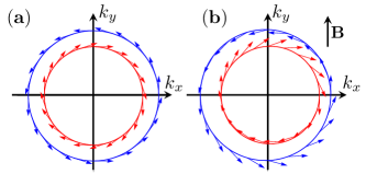
Figure 1: The deformation of the spin texture set by the Rashba spin-orbit interaction by the in-plane field (arbitrary units). The two circles are the Fermi surfaces of the two spin split bands. The arrows stand for the spin polarization at the point of origin. (a) We set $\Delta_{\mathrm{SO}}=0.6E_{F}$ for illustration. (b) An in-plane field $\mathbf{B}=B\hat{y}$ shifts the two Fermi surfaces in the opposite directions. The deformation of the spin textures is the largest along the $k_{y}$ axis, where the combination $\boldsymbol{\gamma}(\mathbf{k})\times\mathbf{B}$ is maximal.

We choose the triplet interaction that is motivated by geometrical arguments. Such triplet interaction arises from the deformation of the spin polarization texture by the Zeeman interaction, see Fig. 1. The deformation at a particular momentum $\mathbf{k}$ is proportional to the cross product, $\boldsymbol{\gamma}(\mathbf{k})\times\mathbf{B}$. This observation allows one to formulate the field induced triplet order parameter for any given spin-orbit interaction [34]. Such field induced triplets have the same transformation properties as the field that induces them.

For the Rashba spin-orbit coupling, Eq. (7), writing $\boldsymbol{\gamma}(\mathbf{k})\times\mathbf{B}=\alpha\hat{z}(\mathbf{B}\cdot\mathbf{k})$ we deduce the following form of the field induced triplet interactions,

$$\mathbf{d}_{\mathbf{k}}^{x}=\hat{z}\cos\varphi\,,\quad\mathbf{d}_{\mathbf{k}}^{y}=\hat{z}\sin\varphi\,,$$ (17)

where we denote $k_{x}=k\cos\varphi$ and $k_{y}=k\sin\varphi$. Eq. (17) signifies that the Zeeman field couples to $p$-wave triplet interaction channel. It is clear that the pair of functions Eq. (17) as well as the pair of the in-lane field components, $\mathbf{B}=(B_{x},B_{y})$ both transform as the $E_{2}$ irreducible representation of $C_{\infty v}$ as expected.

We note in passing that the out-of-plane field belongs to the $A_{2}$ irreducible representation of the same group. The one-component triplets of the $A_{2}$ symmetry of the form, $\mathbf{d}_{\mathbf{k}}=\hat{\mathbf{k}}$ are expected to be essential for the field pointing out of plane. In fact such triplets potentially play an important role in the field induced transition to the odd parity singlet state in the locally noncentrosymmetric CeRh₂As₂ superconductor [39].

Below in Sec. IV we provide all the details of the calculation of the dispersion relation, Eq. (II). For convenience, prior to delving into the details we list the coefficients entering the dispersion relations in the clean and dirty limits in Sec. III.1.

III.1 Summary of the dispersion relation Eq. (II)

We discuss now in turn all terms in the dispersion relation (II) of different order in momentum and field. We give the general result and the expressions in the clean and dirty limits.

III.1.1 Critical temperature suppression

To zero order in both momentum and the field, Eq. (II) describes the critical temperature reduction caused by the applied field,

$$T_{c}-T_{c0}=-4T_{c0}B^{2}\tau\gamma_{2}$$ (18)

where $T_{c0}=T_{c}(B=0)$. Here we have introduced the useful sums over the Matsubara frequencies, $\varepsilon_{n}=2\pi T(n+1/2)$,

$$\gamma_{k} =T\sum_{\varepsilon_{n}>0}\frac{\pi}{\varepsilon_{n}^{2}\left(1+2k\tau\varepsilon_{n}\right)}\,,$$ (19a)

$$u_{k} =T\sum_{\varepsilon_{n}>0}\frac{\pi}{2\varepsilon_{n}^{k}\left(1+2\tau\varepsilon_{n}\right)^{3}\left(1+4\tau\varepsilon_{n}\right)^{2}}\,,$$ (19b)

where $k$ is non-negative integer.

In the clean and dirty limit $\gamma_{k}$, Eq. (19a) attains the values

$$\tau\gamma^{c}_{k}=\frac{2}{k}\frac{[\xi^{c}_{0}]^{2}}{v_{F}^{2}}\,,\,\,\,\tau\gamma^{d}_{k}=2\frac{[\xi^{d}_{0}]^{2}}{v_{F}^{2}}$$ (20)

expressible in terms of the zero field size of the Cooper pairs $\xi_{0}$ in respective limits,

$$\xi_{0}^{c}=\left[\frac{7\zeta(3)v_{F}^{2}}{32\pi^{2}T_{c}^{2}}\right]^{1/2},\,\,\xi_{0}^{d}=\left[\frac{\pi\tau v_{F}^{2}}{16T_{c}}\right]^{1/2}\,.$$ (21)

The clean limit of $\tau\gamma_{2}$ as given by Eq. (20) when substituted to Eq. (18) reproduces the result of Ref. [40]. In the dirty limit, we have instead

$$T_{c}-T_{c0}=-B^{2}\frac{\pi\tau}{2}\,.$$ (22)

Comparison of the clean limit result and Eq. (22) shows that the disorder opposes the pair breaking effect of the in-plane field. This is in contrast to the case of Ising superconductors with $\boldsymbol{\gamma}(\mathbf{k})\parallel\hat{z}$, [41, 32, 42].

The superconducting transition occurs into the helical state with the finite momentum, $\mathbf{q}_{h}=\hat{z}\times\mathbf{B}\mathcal{L}_{1}/2\xi_{0}^{2}$. This, however has negligible effect on the critical temperature.

III.1.2 Lifshitz invariant, $\mathcal{L}_{1}$

The Lifshitz invariant has been obtained previously in Ref. [38, 43],

$$\mathcal{L}_{1}=xv_{F}\tau\gamma_{2}\,.$$ (23)

The clean and dirty limits of Eq. (23) follow from Eqs. (20) and (21). The suppression of $\mathcal{L}_{1}$ caused by the disorder follows from the ratio of $\mathcal{L}^{c,d}_{1}$ in the clean and dirty limits,

$$\frac{\mathcal{L}^{d}_{1}}{\mathcal{L}^{c}_{1}}=\frac{2\pi^{3}}{7\zeta(3)}T_{c}\tau\,.$$ (24)

We stress that a finite result is obtained only if the density of states at the two spin split bands are not the same, $x\neq 0$. The dependence of $\mathcal{L}_{1}$ on the disorder strength and the temperature are the same as that of the $T_{c}$ suppression as both are proportional to $\tau\gamma_{2}$. So stronger pair breaking leads to enhanced $\mathcal{L}_{1}$.

Apart from Eq. (23) there is an additional contribution to $\mathcal{L}_{1}$,

$$\delta\mathcal{L}^{s}_{1}=\frac{1}{|g|\nu_{0}}\frac{1}{k_{F}\Delta_{\mathrm{SO}}}$$ (25)

originating from the modification of the matrix elements of the spin singlet interaction, (III) by the field. This can be interpreted as arising from the field induced deformation of the spin texture, see Fig. 1. Here we underestimate $\mathcal{L}^{s}_{1}$ by ignoring $\log(\omega_{D}/\Delta_{\mathrm{SO}})$ in comparison to $\log(\omega_{D}/T_{c})$. Otherwise Eq. (25) acquires an additional factor of two.

At first glance in the considered range of parameters, Eq. (4), Eq. (25) is smaller than the standard expression, (23) that scales with $T_{c}^{-1}$. Eq. (25) nevertheless can be comparable or even exceed Eq. (23) because it is enhanced by the large factor $1/|g|\nu_{0}$, and Eq. (23) furthermore contains $x\ll 1$. Specifically, in the clean limit, the ratio

$$\frac{\delta\mathcal{L}_{1}^{s}}{\mathcal{L}_{1}^{c}}=\frac{1}{|g|\nu_{0}}\frac{T_{c}^{2}}{\Delta^{2}_{\mathrm{SO}}}\frac{(8\pi)^{2}}{7\zeta(3)}$$ (26)

can be large even within the range, Eq. (4). For instance, taking $\omega_{D}=250$K, $\Delta_{\mathrm{SO}}=50$K Eq. (26) gives $\delta\mathcal{L}^{s}_{1}/\mathcal{L}_{1}^{c}\approx 3.2$ for $g\nu_{0}=0.25$. At the same time $T_{c}\approx 5$K still satisfies the condition, $T_{c}\ll\Delta_{\mathrm{SO}}$. Making the system dirtier further increases the ratio (26). For coupling that is sufficiently weak the rapid decrease in $T_{c}$ makes this ratio inevitably small.

The triplet channel interaction (III) makes a contribution to the Lifshitz invariant that is similar in form to that of the interaction in the singlet channel, Eq. (25),

$$\delta\mathcal{L}^{t}_{1}=2\frac{g^{*}_{t}}{|g|}\delta\mathcal{L}^{s}_{1}\,.$$ (27)

The sign of the correction (27) is the same as the sign of the renormalized triplet interaction amplitude, $g^{*}_{t}$. This amplitude replaces the bare interaction $g_{t}$

Cooper channel renormalization takes the form $g^{*}_{t}=g_{t}[1+\varkappa g_{t}\log(\omega_{D}/\Delta_{\mathrm{SO}})]^{-1}$. Here $\varkappa$ is a numerical constant of order one. The low energy cut-off of the logarithm is $\Delta_{\mathrm{SO}}$ since at $B=0$ and $q=0$ the triplet interaction is purely inter-band. Hence, in the considered range of parameters, $g_{t}^{*}\lesssim g_{t}$, and $|g_{t}^{*}|\gtrsim|g_{t}|$ in case of repulsion and attraction interaction in the triplet channel, respectively. Clearly the ratio $\delta\mathcal{L}^{t}_{1}/\delta\mathcal{L}^{s}_{1}$ depends on the model parameters.

III.1.3 Field dependence of the Cooper pair size, $\xi$

To second order in $B$ we write $\xi^{2}=\xi_{0}^{2}+\xi_{2}^{2}B^{2}$, where up to a small corrections in $x\ll 1$

$$\xi_{0}^{2}=\frac{1}{2}v_{F}^{2}\tau\gamma_{1}\,$$ (28)

is standard, [44]. In the clean and dirty limits, $\xi_{0}$ reduces to $\xi_{0}^{c,d}$ given by Eqs. (21), respectively.

The angular average size of the Cooper pairs decreases in a weak field by an amount,

$$\xi_{2}^{2}=-\rho_{2}-\rho_{1}/4\,,$$ (29)

where as in Eq. (28) we have set $x$ to zero, and introduced

$$\rho_{1}= 2\pi\tau^{2}v_{F}^{2}\left(13\tau u_{2}+72\tau^{2}u_{1}+96\tau^{3}u_{0}\right)\,,$$ (30a)

$$\rho_{2}= \frac{\pi}{2}\tau^{2}v_{F}^{2}\left(4u_{3}+37\tau u_{2}+104\tau^{2}u_{1}+96\tau^{3}u_{0}\right)\,.$$ (30b)

In the clean limit we have

$$\rho^{c}_{1}=93\zeta(5)\left(\frac{4}{7\zeta(3)}\right)^{2}\frac{[\xi^{c}_{0}]^{4}}{v_{F}^{2}}\,,\quad\rho^{c}_{2}=\rho^{c}_{1}/4\,.$$ (31)

In the dirty limit,

$$\rho^{d}_{1}=52\tau^{2}[\xi_{0}^{d}]^{2}\,,\quad\rho^{d}_{2}=\frac{14\zeta(3)}{\pi^{2}}\frac{\tau}{T_{c}}[\xi_{0}^{d}]^{2}\,.$$ (32)

III.1.4 The field induced anisotropy

The field induced anisotropy of the Cooper pairs is encapsulated in the $\mathcal{L}_{2}$ coefficient,

$$\mathcal{L}_{2}=\rho_{1}/4\,.$$ (33)

Based on Eqs. (31) and (32) we have for the ratio of the anisotropy coefficient in the clean and dirty limits,

$$\frac{\mathcal{L}^{d}_{2}}{\mathcal{L}^{c}_{2}}=(\tau T_{c})^{3}\frac{206\pi^{5}}{93\zeta(5)}\,.$$ (34)

Eq. (34) indicates that the disorder suppresses the planar Hall effect. This is to be expected as the disorder tends to restore the isotropy of the dispersion relation of the Cooper pairs.

Similar to the case of the Lifshitz invariant the variation of the matrix elements of the singlet pairing interaction as well as the $p$-wave triplet interaction introduce corrections to $\mathcal{L}_{2}$. These corrections read

$$\delta\mathcal{L}_{2}^{s}=\frac{1}{|g|\nu_{0}}\frac{c^{s}_{2}}{k_{F}^{2}\Delta_{\mathrm{SO}}^{2}}\,,\quad\delta\mathcal{L}^{t}_{2}=c_{2}^{t}\frac{g^{*}_{t}}{|g|}\delta\mathcal{L}^{s}_{2}\,,$$ (35)

respectively with a numerical constants $c_{2}^{s,t}$. Unlike in the case of $\mathcal{L}_{1}$ these corrections are small,

$$\frac{\delta\mathcal{L}_{2}^{s,t}}{\mathcal{L}_{2}}\propto\frac{1}{|g|\nu_{0}}\left(\frac{T_{c}}{E_{F}}\right)^{2}\left(\frac{T_{c}}{\Delta_{\mathrm{SO}}}\right)^{2}\,.$$ (36)

In contrast to the ratio, Eq. (26), the ratio Eq. (36) contains an extra small parameter $(T_{c}/E_{F})^{2}$. This makes the contributions Eq. (35) irrelevant. The reason for this difference is that in contrast to $\mathcal{L}_{2}$, $\mathcal{L}_{1}$ hinges on the finite difference of the density of states at the two spin split Fermi surfaces. This increases the relative importance of the corrections $\delta\mathcal{L}_{1}^{s,t}$.

IV Calculation of the dispersion of the Cooper pairs

In this section we perform the calculation of the Cooper pair dispersion, Eq. (II). For now we focus on the pairing in the s-wave singlet channel. At the latter stage we analyze the additional contributions due to the triplet channel interaction. Introduce the correlation function for the Cooper pairs at the momentum $\mathbf{q}$ and bosonic Matsubara frequency, $\Omega_{n}=2\pi Tn$ [35],

$$K \left(\mathbf{q},i\Omega_{m}\right)=\sum_{\mathbf{k},\mathbf{k}^{\prime},s}\int_{0}^{T^{-1}}d\tau\exp(i\Omega_{n}\tau)$$

$$\times \Big{\langle}T_{\tau}\big{\{}c_{-\mathbf{k}_{-}s_{1}}(\tau)\left[i\sigma_{y}\right]^{\dagger}_{s_{1}s_{2}}c_{\mathbf{k}_{+}s_{2}}(\tau)$$

$$\times c_{\mathbf{k}^{\prime}_{+}s_{1}}^{\dagger}(\tau)\left[i\sigma_{y}\right]_{s_{1},s_{2}}c_{-\mathbf{k}^{\prime}_{-}s_{2}}^{\dagger}(\tau)\big{\}}\Big{\rangle}\,,$$ (37)

where $T_{\tau}$ stands for the time ordering in the imaginary time $\tau$, and for any operator $O$, $O(\tau)=\exp(H\tau)O\exp(-H\tau)$.

The dynamic properties of the Cooper pairs are contained in the retarded correlation functions obtained form (IV) via the analytic continuation, $i\Omega_{n}\rightarrow\Omega+i0_{+}$. In this work we assume that the dependence of the Cooper pair propagators on the frequency $\Omega$ at $\Omega\lesssim T-T_{c}\ll T_{c}$ is unaffected by the magnetic field and the spin orbit interaction. Under this condition we take the Cooper pairs dissipation rate $\gamma_{\text{GL}}$ in Eq. (1) as in the standard BCS theory. This assumption holds under the conditions (4). We therefore set $\Omega_{n}=0$ in Eq. (IV) above.

In the weak coupling regime, $g\nu_{0}\ll 1$ the correlation function (IV) takes the standard form

$$K\left(\mathbf{q},i\Omega_{m}\right)=\frac{\Pi_{\mathbf{q}}\left(i\Omega_{m}\right)}{1+(g/4)\Pi_{\mathbf{q}}\left(i\Omega_{m}\right)}\,,$$ (38)

where the polarization operator, $\Pi_{\mathbf{q}}$ is the correlation function, $K$ in the non-interacting limit, $g=0$.

The dispersion relation is given by the inverse correlation function (IV),

$$\nu_{0}\varepsilon_{\mathbf{q}}=1/g+\Pi_{\mathbf{q}}/4\,,$$ (39)

where as before the order parameter is normalized to be a equal to the gap function at equilibrium.

IV.1 Chiral basis formulation

The calculation of the Cooper pair dispersion, (39) is performed in the chiral basis, Eq. (12). This is done in two steps. First we perform the transformation to the basis, Eq. (10) that diagonalizes the free part of the Hamiltonian (5) including Eqs. (6), (7) and (8). Second, one performs the expansion of the dispersion relation (39) in $B$. As $B$ is set to zero, the generic basis Eq. (10) turns into the chiral basis, Eq. (12).

The transformation to the basis, Eq. (10) has an advantage of making the Green function matrix diagonal, $G_{\lambda\lambda^{\prime}}=\delta_{\lambda\lambda^{\prime}}G_{\lambda}$ even at finite $B$. The diagonal elements of the Green function read,

$$G_{\lambda}(\mathbf{k},\varepsilon_{n})=\left[i\varepsilon_{n}-\xi^{\lambda}_{k}-\mathbf{v}_{F}\cdot\mathbf{Q}^{\lambda}+i\frac{\mathrm{sgn}(\varepsilon_{n})}{2\tau}\right]^{-1}\,,$$ (40)

where

$$\mathbf{Q}^{\lambda}=\mathbf{q}/2+\lambda\hat{z}\times\mathbf{B}/v_{F}\,.$$ (41)

We note that the diagonal form of the Green function presumed by the Eq. (40) is preserved by the disorder potential only if the disorder potential does not mix spin split bands. This imposes the condition $\max\{1/\tau,T_{c}\}\ll\Delta_{\mathrm{SO}}$ included in Eq. (4).

To encompass the effect of the disorder we express the Cooper pair propagator in terms of the Green functions and the Cooperon vertex, $\overline{\Gamma}^{\lambda}_{\lambda^{\prime}}(\mathbf{k},\mathbf{q},\mathbf{B},\varepsilon_{n})$, see Fig. 2,

$$\!\Pi_{\mathbf{q}}\!=\!2T\!\!\sum_{\mathbf{k},\varepsilon_{n}\lambda\lambda^{\prime}}\!\!\left[i\check{\sigma}_{y}(\mathbf{k},\mathbf{q},\mathbf{B})\right]_{\lambda\lambda^{\prime}}\mathbb{G}^{\lambda}_{\lambda^{\prime}}\left(\mathbf{k},\mathbf{q},\mathbf{B},\varepsilon_{n}\right)\overline{\Gamma}^{\lambda}_{\lambda^{\prime}}\,,$$ (42)

where the combinatorial factor of 2 is included and,

$$\mathbb{G}^{\lambda}_{\lambda^{\prime}}\left(\mathbf{k},\mathbf{q},\mathbf{B},\varepsilon_{n}\right)=G_{\lambda}\left(\mathbf{k}_{+},\varepsilon_{n}\right)G_{\lambda^{\prime}}\left(-\mathbf{k}_{-},-\varepsilon_{n}\right)\,,$$ (43)

and $\left[i\check{\sigma}_{y}(\mathbf{k},\mathbf{q},\mathbf{B})\right]$ stands for the interaction vertex of the interaction Hamiltonian Eq. (III) in the basis, Eq. (10). It defined such that the interaction Hamiltonian, (III) takes the form

$$H_{p}^{s}= \frac{g}{4}\sum_{\mathbf{k},\mathbf{k}^{\prime},\mathbf{q};\lambda}\left\{\hat{\psi}_{\mathbf{B}}^{\lambda_{1}\dagger}(\mathbf{k}_{+})\left[i\check{\sigma}_{y}\right]_{\lambda_{1},\lambda_{2}}\hat{\psi}_{\mathbf{B}}^{\lambda_{2}\dagger}(-\mathbf{k}_{-})\right\}$$

$$\times\left\{\hat{\psi}_{\mathbf{B}}^{\lambda_{3}}(-\mathbf{k}^{\prime}_{-})\left[i\check{\sigma}_{y}\right]^{\dagger}_{\lambda_{3}\lambda_{4}}\hat{\psi}_{\mathbf{B}}^{\lambda_{4}}(\mathbf{k}^{\prime}_{+})\right\}\,.$$ (44)

Naturally, $\left[i\check{\sigma}_{y}(\mathbf{k},\mathbf{q},\mathbf{B})\right]$ vertex takes a more complex form of Eq. (A) than just $i\sigma_{y}$ in the original basis, Eq. (III). We will see, however, that since the interaction vertex depends on the two small parameters, $q/k_{F}\ll 1$ and $B/\Delta_{\mathrm{SO}}\ll 1$ it is greatly simplified in the studied limit.

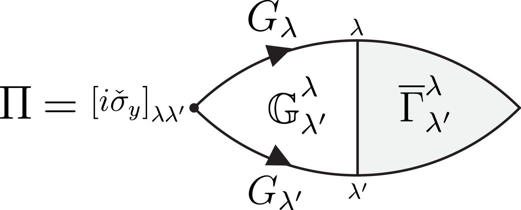
Figure 2: Diagrammatic presentation of the equation (42) defining the effect of the disorder on the fluctuation spectrum. $\mathbb{G}^{\lambda}_{\lambda^{\prime}}$ is introduced in Eq. (43), and $\Gamma^{\lambda}_{\lambda^{\prime}}$ stands for the Cooperon vertex.

In contrast to the interaction vertex in Eq. (42), the second factor, $\mathbb{G}^{\lambda}_{\lambda^{\prime}}$ depends on the momentum and the field via the dimensionless parameters, $qv_{F}/\max\{T_{c},1/\tau\}$ and $B/\max\{T_{c},1/\tau\}$. Because as stated in Eq. (4), $\max\{T_{c},1/\tau\}\ll\Delta_{\mathrm{SO}}$ and $T_{c}\ll E_{F}$ we can discard the momentum and the field dependence of $i\check{\sigma}_{y}(\mathbf{k},\mathbf{q},\mathbf{B})$ and keep it only in the $\mathbb{G}^{\lambda}_{\lambda^{\prime}}$. As detailed in App. A.1, to zero order in $q/k_{F}$ and $B/\Delta_{\mathrm{SO}}$, the interaction vertex,

$$\left[i\check{\sigma}_{y}(\mathbf{k})\right]_{\lambda\lambda^{\prime}}=i\lambda\delta_{\lambda\lambda^{\prime}}e^{i\varphi}\,$$ (45)

is purely intra-band.

IV.2 Cooperon vertex renormalization

The Cooperon vertex introduced in Eq. (42) satisfies the integral equation, see Fig. 3,

$$\overline{\Gamma}^{\lambda}_{\lambda^{\prime}} \left(\mathbf{k},\mathbf{q},\mathbf{B},\varepsilon_{n}\right)=\left[i\check{\sigma}_{y}\right]_{\lambda\lambda^{\prime}}+\sum_{\mathbf{p}^{\prime}\eta\eta^{\prime}}{}^{\lambda}_{\lambda^{\prime}}\!\tilde{V}^{\eta}_{\eta^{\prime}}\left(\mathbf{k},\mathbf{k}^{\prime}\right)$$

$$\times\mathbb{G}^{\eta}_{\eta^{\prime}}\left(\mathbf{k}^{\prime},\mathbf{q},\mathbf{B},\varepsilon_{n}\right)\overline{\Gamma}^{\eta}_{\eta^{\prime}}\left(\mathbf{k}^{\prime},\mathbf{q},\mathbf{B},\varepsilon_{n}\right)\,,$$ (46)

where $\tilde{V}$ is the scattering vertex in the chiral basis. All the important electron momenta are close to $k_{F}$. For such momenta we have

$${}^{\lambda}_{\lambda^{\prime}}\!\tilde{V}^{\eta}_{\eta^{\prime}}\left(\mathbf{k},\mathbf{k}^{\prime}\right)\approx \frac{V^{2}}{4}\left[1+\lambda\eta e^{-i\left(\varphi-\varphi^{\prime}\right)}\right]$$

$$\times\left[1+\lambda^{\prime}\eta^{\prime}e^{-i\left(\varphi-\varphi^{\prime}\right)}\right]\,.$$ (47)

This equation holds under the same conditions as Eq. (45), see App. B.

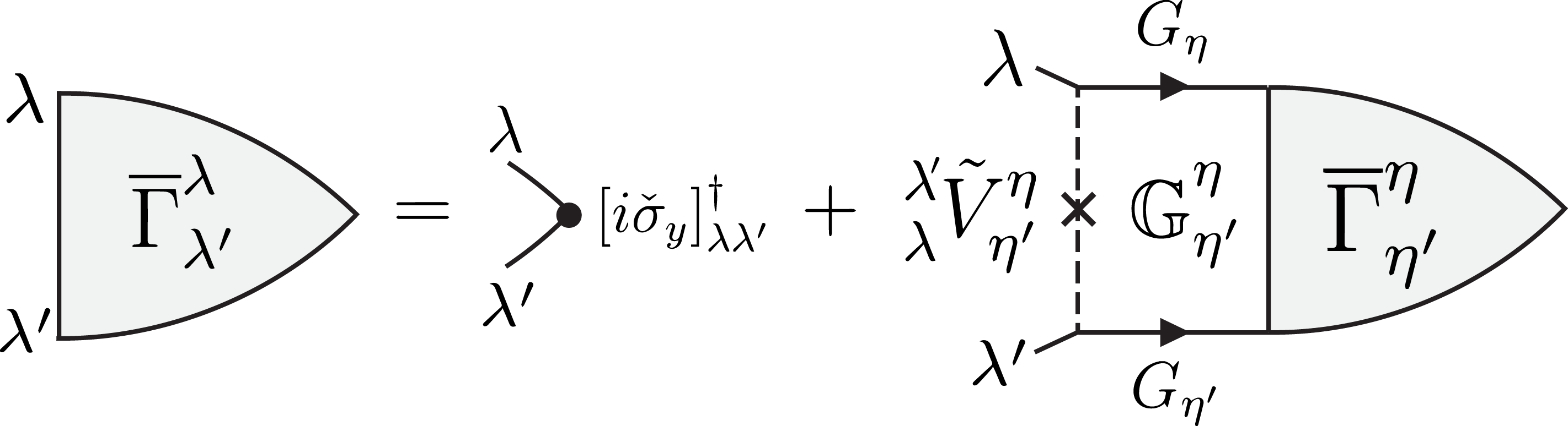
Figure 3: Diagrammatic presentation of the integral equation (IV.2) satisfied by the Cooperon vertex, $\overline{\Gamma}$. The disorder scattering vertex, $\tilde{V}$, is defined in Eq. (IV.2), and $\mathbb{G}$ stands for the product of the two Green functions, see Eq. (43).

As discussed in App. C the inter-band scattering processes captured by Eq. (IV.2) by the terms with $\eta\neq\eta^{\prime}$ give a negligible contribution under the condition $\max\{1/\tau,T_{c}\}\ll\Delta_{\mathrm{SO}}$. This restriction is consistent with the Green function, Eq. (40) being diagonal in the band index. The above condition, in fact ensures the two spin split bands can be treated as a two-band superconductor. In this approximation the inter-band pairing has a negligible effect.

Considering only the intra-band Cooper pairs we follow the standard route by integrating over fast electron momentum introducing the integral,

$$\overline{\mathbb{G}}_{\lambda}^{\lambda}\left(\varphi,\mathbf{q},\mathbf{B},\varepsilon_{n}\right)= \nu_{\lambda}\int_{-\infty}^{\infty}d\xi_{\mathbf{k}}^{\lambda}\mathbb{G}_{\lambda}^{\lambda}\left(\mathbf{k},\mathbf{q},\mathbf{B},\varepsilon_{n}\right)$$

$$= \frac{2\pi\nu_{\lambda}}{2|\varepsilon_{n}|+2i\mathbf{v}_{F}\cdot\mathbf{Q}^{\lambda}+\frac{\mathrm{sgn}(\varepsilon_{n})}{\tau}}.$$ (48)

The integration in Eq. (IV.2) has an effect of setting all the electron momenta to the Fermi momentum. In result, keeping only intra-band contributions, Eq. (IV.2) is transformed to

$$\overline{\Gamma}^{\lambda}_{\lambda} \left(\varphi,\mathbf{q},\mathbf{B},\varepsilon_{n}\right)=\left[i\check{\sigma}_{y}\left(\varphi\right)\right]_{\lambda\lambda}+\int\frac{d\varphi^{\prime}}{2\pi}\sum_{\eta}{}^{\lambda}_{\lambda}\!\tilde{V}^{\eta}_{\eta}\left(\varphi-\varphi^{\prime}\right)$$

$$\times\overline{\mathbb{G}}^{\eta}_{\eta}\left(\varphi^{\prime},\mathbf{q},\mathbf{B},\varepsilon_{n}\right)\overline{\Gamma}^{\eta}_{\eta}\left(\varphi^{\prime},\mathbf{q},\mathbf{B},\varepsilon_{n}\right)\,.$$ (49)

It is convenient to introduce the modified vertex function,

$$\Gamma_{\lambda}(\varphi)=ie^{i\varphi}\overline{\Gamma}^{\lambda}_{\lambda}(\varphi).$$ (50)

and the modified disorder scattering vertex,

$${}^{\lambda}_{\lambda}{\tilde{V}}^{\eta}_{\eta}\left(\varphi-\varphi^{\prime}\right)={\left[V_{0}\right]}_{\lambda\eta}\left(\varphi-\varphi^{\prime}\right)\,.\left[e^{i(\varphi^{\prime}-\varphi)}\right]\,.$$ (51)

Multiplying Eq. (IV.2) by $-ie^{-i\varphi}$, and using the definitions (50) and (51) we write it in the form,

$$\Gamma_{\lambda}\left(\varphi\right)= \lambda+\sum_{\eta}\int_{0}^{2\pi}\frac{d\varphi^{\prime}}{2\pi}{\left[V_{0}\right]}_{\lambda\eta}\left(\varphi-\varphi^{\prime}\right)$$

$$\times\overline{\mathbb{G}}^{\eta}_{\eta}\left(\varphi^{\prime}\right)\Gamma_{\eta}\left(\varphi^{\prime}\right)\,$$ (52)

illustrated graphically in Fig. 4. The disorder scattering vertex $V_{0}$ in Eq. (IV.2) is fixed by Eqs. (IV.2) and (51),

$${\left[V_{0}\right]}_{\lambda\eta}=\frac{V^{2}}{2}\left[\cos\left(\varphi-\varphi^{\prime}\right)+\lambda\eta\right]\,.$$ (53)

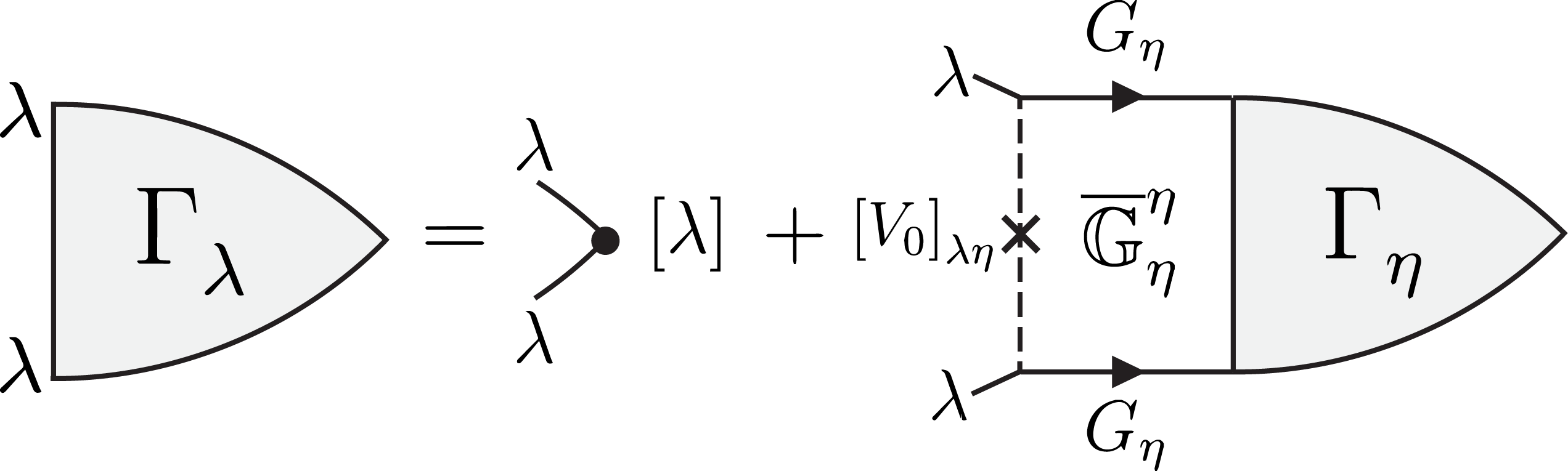
Figure 4: Diagrammatic representation of the integral equation (IV.2) satisfied by the modified Cooperon vertex, $\Gamma$. The disorder scattering amplitude $V_{0}$ is defined by Eq. (53). The integrated product of the two Green functions, $\bar{\mathbb{G}}$ is given by Eq. (IV.2).

It is clear from Eq. (IV.2) and the form of the disorder scattering amplitude, Eq. (53) that the solution to the Eq. (IV.2) takes the form,

$$\Gamma_{\lambda}\left(\varphi\right) =C_{\lambda}^{\left(0\right)}+C_{\lambda}^{\left(c\right)}\cos\varphi+C_{\lambda}^{\left(s\right)}\sin\varphi\,.$$ (54)

The specific form of Eq. (54) turns equation (IV.2) into six linear algebraic equations for the six unknown coefficients $C_{\pm}^{\left(0\right)}$, $C_{\pm}^{\left(c\right)}$, and $C_{\pm}^{\left(s\right)}$. These equations can be summarized as follows. Introduce the column vector,

$$\mathbf{C}=\left[C_{+}^{\left(0\right)},C_{+}^{\left(c\right)},C_{+}^{\left(s\right)},C_{-}^{\left(0\right)},C_{-}^{\left(c\right)},C_{-}^{\left(c\right)}\right]^{\mathrm{t}}\,,$$ (55)

where the superscript $\mathrm{t}$ stands for the transposition. The linear equation satisfied by $\mathbf{C}$ takes the form,

$$\left(\mathbb{M}-\mathbb{1}_{6}\right)\mathbf{C}=\left[-1,0,0,1,0,0\right]^{\mathrm{t}}\,,$$ (56)

where $\mathbb{1}_{6}$ is the six by six unit matrix, and $\mathbb{M}$ can be written as the two by two matrix

$$\mathbb{M}=\begin{bmatrix}A_{+}&A^{\prime}_{-}\\ A^{\prime}_{+}&A_{-}\end{bmatrix}\,$$ (57)

with entries that are three by three matrices,

$$A_{\lambda}=\begin{bmatrix}A_{\lambda}^{00}&A_{\lambda}^{10}&A_{\lambda}^{01}\\ A_{\lambda}^{10}&A_{\lambda}^{20}&A_{\lambda}^{11}\\ A_{\lambda}^{01}&A_{\lambda}^{11}&A_{\lambda}^{02}\end{bmatrix}\,,$$ (58)

where

$$A_{\lambda}^{mn}=\frac{V^{2}}{2}\int_{0}^{2\pi}\frac{d\varphi}{2\pi}\overline{\mathbb{G}}^{\lambda}_{\lambda}\left(\varphi\right)\cos^{m}\varphi\sin^{n}\varphi\,.$$ (59)

In Eq. (57) $A^{\prime}_{\lambda}$ differ from $A_{\lambda}$ by a sign of the entries in the first row of the defining Eq. (58).

To complete the calculation, we rewrite the expression for the polarization operator Eq. (42) within the approximations made above in the form, see Fig. 5,

$$\Pi_{\mathbf{q}}=2T\sum_{\varepsilon_{n}}\int_{0}^{2\pi}\frac{d\varphi}{2\pi}\left(\overline{\mathbb{G}}^{+}_{+}\Gamma_{+}-\overline{\mathbb{G}}^{-}_{-}\Gamma_{-}\right)\,.$$ (60)

We have checked that at $q=0$ and $B=0$, Eq. (60) reduces to the expression, $\Pi_{\mathbf{q}}=4\pi\nu_{0}/|\varepsilon_{n}|$ which does not include the disorder in accordance with the Anderson theorem.

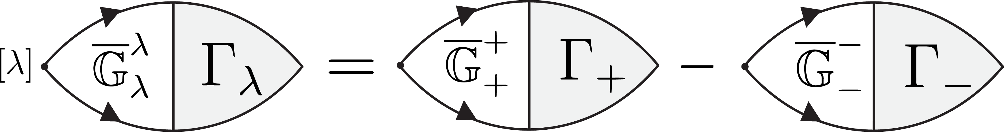
Figure 5: Diagrammatic presentation of the expression (60) for the polarization operator $\Pi_{\mathbf{q}}$. The integrated product of the two Green functions $\bar{\mathbb{G}}$ is given by Eq. (IV.2). The Cooperon vertex, $\Gamma$, satisfies the integral Eq. (IV.2) illustrated in Fig. 4.

The outline of the remaining calculation is as follows. We solve the Eq. (56). This gives the Cooperon vertex via the expansion, Eq. (54). This solution, in turn, allows us to evaluate the polarization operator using Eq. (60). The knowledge of $\Pi_{\mathbf{q}}$ translates directly into the Cooper pair dispersion, Eq. (39).

The calculations are performed to the fourth order in $\mathbf{Q}^{\lambda}$. This implies according to the definition (41) that we keep all the terms in the Cooper pair dispersion to the order $n_{q}$ in $q$ and $n_{B}$ in $B$ such that $n_{q}+n_{B}\leq 4$. Clearly, such procedure is sufficient to obtain all the terms in the expression (II). Each of the coefficients in Eq. (II) is given in Sec. III.1 in clean and dirty limits.

V Discussion and outlook

We have studied the way superconducting fluctuations lead to the two-fold magneto-resistance anisotropy in the form of the PHE. We have focused on the paradigmatic model of the Rashba-Zeeman superconductor in the metallic regime, $E_{F}\gg\Delta_{\mathrm{SO}}$. In this limit, the PHE vanishes in the absence of interactions and at a non-zero disorder concentration.

In contrast, interactions in the Cooper pairing channel produce a finite contribution to PHE. This makes the paraconductivity due to the superconducting fluctuations the primary source of the two-fold magneto-resistance anisotropy in spin-orbit coupled systems. More specifically, the PHE results from the anisotropy of the dispersion relation of the Cooper pairs. Such anisotropy is only moderately suppressed by disorder.

We have limited the consideration to large spin-orbit splitting, Eq. (4) where the Rashba-Zeeman superconductor can be effectively described as a two-band superconductor. This statement in the present approach amounts to the inter-band pairing making a negligible contribution the Cooper pair dispersion. Indeed, the Cooper pair anisotropy can be safely calculated within this approximation.

The interaction matrix elements in the effective two-band theory generally depend on the Cooper pair momentum and the applied field. Such dependence is nominally weak and can be ignored in most situations. This, however, may not be the case when one specifically considers the Lifshitz invariant, linear in field and momentum. Within the two-band approximation it builds on the finite difference in the density of states at the two spin split Fermi surfaces, and it scales, therefore, with $\Delta_{\mathrm{SO}}/E_{F}\ll 1$. Because of this smallness, the field dependence of the interaction matrix elements can make a comparable or even bigger contribution to the Lifshitz invariant if $T_{c}\ll\Delta_{\mathrm{SO}}\lesssim T_{c}/\sqrt{|g|\nu_{0}}$.

The above field dependence of interaction matrix elements originates from the deformation of the spin texture of the two spin split bands, see Fig. 1. This adjustment gives rise to yet another effect, contributing, again, to the Lifshitz invariant. It allows certain triplet correlations to affect the spin singlet Cooper pairs at finite field. In Rashba-Zeeman system such field induced triplet state have a $p$-wave symmetry. As the spin texture is deformed by the field, the $p$-wave triplet Cooper pairs gradually turn into the $s$-wave spin-singlet Cooper pairs. Such a conversion is mediated by the Rashba spin-orbit interaction. The repulsion or attraction in this specific triplet channel makes a contribution to the Lifshitz invariant similar to that of the singlet channel.

In contrast to the Lifshitz invaraint, the PHE is not sensitive to the difference in the density of states at the two spin split Fermi surfaces. In result, we have found that the PHE can be safely studied within the two-band approximation, in the limit, $\Delta_{\mathrm{SO}}\gg T_{c}$. Namely, as far as the PHE is concerned, one can ignore the field dependence of the attraction interaction in singlet channel as well as the contribution of the triplet channel. We speculate that this is not the case in the opposite regime, $\Delta_{\mathrm{SO}}\ll T_{c}$.

Our results bear implications on the PHE in the topological surface states. The present derivation applies as is to the metallic regime with the Fermi energy far above or below the Dirac point. Indeed, in this regime the electron dispersion becomes similar to the one in the Rashba-Zeeman system. Yet, even close to Dirac point the superconducting fluctuations have a potential to appreciably modify the PHE. In particular, the triplet correlations have a potential to play an important role due to the spin-orbit coupling being the dominant energy scale at the charge neutrality.

We note that the interaction matrix elements may exhibit a non-analytic momentum dependence at a special configuration with equal spin-orbit and Zeeman splitting. In this case the two spin split Fermi surfaces touch, see Fig. 1. At the same configuration the applied field drives the topological transition of the spin texture. This unusual regime, however, can be reached if $T_{c}\gg\Delta_{\mathrm{SO}}$ which is the opposite limit of the effective two-band theory considered in this work. It is left for future investigations.

Appendix A Pairing interaction Hamiltonian in the basis, Eq. (10)

In this section we transform the singlet pairing interaction Hamiltonian, Eq. (III) to the basis, Eq. (10) that diagonalizes the free part of the Hamiltonian. We then show that to the zero-order expansion in $q/k_{F},B/\Delta_{\mathrm{SO}}\ll 0$, the interaction vertex is given by Eq. (45). This procedure amounts to transformation to the chiral basis, Eq. (12). For completeness we do it in two steps. First transform to the basis, Eq. (10), and second reduce it to the transformation to the basis, Eq. (12). The inverse transformation Eq. (III) implies

$$\hat{c}^{\dagger}_{\uparrow} \left(\mathbf{k}+\frac{\mathbf{q}}{2}\right)\!=\!\frac{1}{\sqrt{2}}\left[\hat{\psi}_{\mathbf{B}}^{+{\dagger}}\left(\mathbf{k}+\frac{\mathbf{q}}{2}\right)\!+\!\hat{\psi}_{\mathbf{B}}^{-{\dagger}}\left(\mathbf{k}+\frac{\mathbf{q}}{2}\right)\right]$$ (61a)

$$\hat{c}^{\dagger}_{\downarrow} \left(\mathbf{k}+\frac{\mathbf{q}}{2}\right)=\frac{1}{\sqrt{2}}\left[\hat{\psi}_{\mathbf{B}}^{+{\dagger}}\left(\mathbf{k}+\frac{\mathbf{q}}{2}\right)-\hat{\psi}_{\mathbf{B}}^{-{\dagger}}\left(\mathbf{k}+\frac{\mathbf{q}}{2}\right)\right]$$

$$\times\left[\frac{\left(k_{y}+\frac{q_{y}}{2}+\frac{B_{x}}{\alpha}\right)-i\left(k_{x}+\frac{q_{x}}{2}-\frac{B_{y}}{\alpha}\right)}{\sqrt{\left(k_{x}+\frac{q_{x}}{2}-\frac{B_{y}}{\alpha}\right)^{2}+\left(k_{y}+\frac{q_{y}}{2}+\frac{B_{x}}{\alpha}\right)^{2}}}\right]$$ (61b)

and similarly

$$\hat{c}_{\uparrow}\! \!\left(\mathbf{k}^{\prime}+\frac{\mathbf{q}}{2}\right)=\frac{1}{\sqrt{2}}\left[\hat{\psi}^{+}_{\mathbf{B}}\left(\mathbf{k}^{\prime}\!+\!\frac{\mathbf{q}}{2}\right)+\hat{\psi}^{-}_{\mathbf{B}}\left(\mathbf{k}^{\prime}\!+\!\frac{\mathbf{q}}{2}\right)\right]$$ (62a)

$$\hat{c}_{\downarrow} \left(\mathbf{k}^{\prime}+\frac{\mathbf{q}}{2}\right)=\frac{1}{\sqrt{2}}\left[\hat{\psi}^{+}_{\mathbf{B}}\left(\mathbf{k}^{\prime}+\frac{\mathbf{q}}{2}\right)-\hat{\psi}^{-}_{\mathbf{B}}\left(\mathbf{k}^{\prime}+\frac{\mathbf{q}}{2}\right)\right]$$

$$\times\left[\frac{\left(k_{y}^{\prime}+\frac{q_{y}}{2}+\frac{B_{x}}{\alpha}\right)+i\left(k_{x}^{\prime}+\frac{q_{x}}{2}-\frac{B_{y}}{\alpha}\right)}{\sqrt{\left(k_{x}^{\prime}+\frac{q_{x}}{2}-\frac{B_{y}}{\alpha}\right)^{2}+\left(k_{y}^{\prime}+\frac{q_{y}}{2}+\frac{B_{x}}{\alpha}\right)^{2}}}\right].$$ (62b)

We, therefore, have based on Eq. (61),

$$\hat{c}^{\dagger}_{\uparrow}\left(\mathbf{k}+\frac{\mathbf{q}}{2}\right)\left[i\sigma_{y}\right]_{\uparrow\downarrow}\hat{c}^{\dagger}_{\downarrow}\left(-\mathbf{k}+\frac{\mathbf{q}}{2}\right)$$

$$=\frac{1}{2}\left[\hat{\psi}^{+{\dagger}}_{\mathbf{B}}\left(\mathbf{k}+\frac{\mathbf{q}}{2}\right)+\hat{\psi}^{-{\dagger}}_{\mathbf{B}}\left(\mathbf{k}+\frac{\mathbf{q}}{2}\right)\right]$$

$$\times\left[\hat{\psi}^{+{\dagger}}_{\mathbf{B}}\left(-\mathbf{k}+\frac{\mathbf{q}}{2}\right)-\hat{\psi}^{-{\dagger}}_{\mathbf{B}}\left(-\mathbf{k}+\frac{\mathbf{q}}{2}\right)\right]$$

$$\times\left[\frac{\left(-k_{y}+\frac{q_{y}}{2}+\frac{B_{x}}{\alpha}\right)-i\left(-k_{x}+\frac{q_{x}}{2}-\frac{B_{y}}{\alpha}\right)}{\sqrt{\left(-k_{x}+\frac{q_{x}}{2}-\frac{B_{y}}{\alpha}\right)^{2}+\left(-k_{y}+\frac{q_{y}}{2}+\frac{B_{x}}{\alpha}\right)^{2}}}\right]$$ (63)

and similarly,

$$\hat{c}^{\dagger}_{\downarrow}\left(\mathbf{k}+\frac{\mathbf{q}}{2}\right)\left[i\sigma_{y}\right]_{\downarrow\uparrow}\hat{c}^{\dagger}_{\uparrow}\left(-\mathbf{k}+\frac{\mathbf{q}}{2}\right)$$

$$=-\frac{1}{2}\left[\hat{\psi}^{+{\dagger}}_{\mathbf{B}}\left(\mathbf{k}+\frac{\mathbf{q}}{2}\right)-\hat{\psi}^{-{\dagger}}_{\mathbf{B}}\left(\mathbf{k}+\frac{\mathbf{q}}{2}\right)\right]$$

$$\times\left[\hat{\psi}^{+{\dagger}}_{\mathbf{B}}\left(-\mathbf{k}+\frac{\mathbf{q}}{2}\right)+\hat{\psi}^{-{\dagger}}_{\mathbf{B}}\left(-\mathbf{k}+\frac{\mathbf{q}}{2}\right)\right]\times$$

$$\times\left[\frac{\left(k_{y}+\frac{q_{y}}{2}+\frac{B_{x}}{\alpha}\right)-i\left(k_{x}+\frac{q_{x}}{2}-\frac{B_{y}}{\alpha}\right)}{\sqrt{\left(k_{x}+\frac{q_{x}}{2}-\frac{B_{y}}{\alpha}\right)^{2}+\left(k_{y}+\frac{q_{y}}{2}+\frac{B_{x}}{\alpha}\right)^{2}}}\right].$$ (64)

The sum of the two contributions, Eqs. (A) and (A) gives rise to the vertex in the basis, Eq. (10),

$$\left[i\check{\sigma}_{y}\left(\mathbf{k},\mathbf{q},\mathbf{B}\right)\right]_{\lambda\lambda^{\prime}}=$$

$$-\frac{1}{2}\left[\lambda\frac{\left(k_{y}+\frac{q_{y}}{2}+\frac{B_{x}}{\alpha}\right)-i\left(k_{x}+\frac{q_{x}}{2}-\frac{B_{y}}{\alpha}\right)}{\sqrt{\left(k_{x}+\frac{q_{x}}{2}-\frac{B_{y}}{\alpha}\right)^{2}+\left(k_{y}+\frac{q_{y}}{2}+\frac{B_{x}}{\alpha}\right)^{2}}}\right.$$

$$- \lambda^{\prime}\left.\frac{\left(-k_{y}+\frac{q_{y}}{2}+\frac{B_{x}}{\alpha}\right)-i\left(-k_{x}+\frac{q_{x}}{2}-\frac{B_{y}}{\alpha}\right)}{\sqrt{\left(k_{x}-\frac{q_{x}}{2}+\frac{B_{y}}{\alpha}\right)^{2}+\left(k_{y}-\frac{q_{y}}{2}-\frac{B_{x}}{\alpha}\right)^{2}}}\right].$$ (65)

Repeating the same steps for the annihilation operators, Eq. (62) we obtain the result,

$$\left[i\check{\sigma}_{y}\left(\mathbf{k}^{\prime},\mathbf{q},\mathbf{B}\right)\right]_{\lambda\lambda^{\prime}}^{\dagger}=$$

$$-\frac{1}{2}\left[\lambda\frac{\left(k^{\prime}_{y}+\frac{q_{y}}{2}+\frac{B_{x}}{\alpha}\right)+i\left(k^{\prime}_{x}+\frac{q_{x}}{2}-\frac{B_{y}}{\alpha}\right)}{\sqrt{\left(k^{\prime}_{x}+\frac{q_{x}}{2}-\frac{B_{y}}{\alpha}\right)^{2}+\left(k^{\prime}_{y}+\frac{q_{y}}{2}+\frac{B_{x}}{\alpha}\right)^{2}}}\right.$$

$$- \lambda^{\prime}\left.\frac{\left(-k^{\prime}_{y}+\frac{q_{y}}{2}+\frac{B_{x}}{\alpha}\right)+i\left(-k^{\prime}_{x}+\frac{q_{x}}{2}-\frac{B_{y}}{\alpha}\right)}{\sqrt{\left(k^{\prime}_{x}-\frac{q_{x}}{2}+\frac{B_{y}}{\alpha}\right)^{2}+\left(k^{\prime}_{y}-\frac{q_{y}}{2}-\frac{B_{x}}{\alpha}\right)^{2}}}\right].$$ (66)

A.1 Approximate expression for the interaction amplitude

As is explained in the main text, in the regime considered in this work it is sufficient to keep the interaction vertices, Eqs. (A) and (A) to zero order in $q/k_{F}$ and $B/\Delta_{\mathrm{SO}}$. Writing the momentum $\mathbf{k}=k\hat{x}\cos\varphi+k\hat{y}\sin\varphi$ as in the main text, we reduce the interaction vertices to the following expressions,

$$\left[i\check{\sigma}_{y}\left(\varphi\right)\right] =ie^{i\varphi}\sigma_{z}$$ (67a)

$$\left[i\check{\sigma}_{y}\left(\varphi^{\prime}\right)\right]^{\dagger} =-ie^{-i\varphi^{\prime}}\sigma_{z}\,.$$ (67b)

Crucially, the interaction amplitude in the chiral representation are purely intra-band.

Appendix B Disorder scattering vertex

Here we transform the disorder Hamiltonian, and the disorder scattering vertex to the basis Eq. (10). As in the case of interaction, we proceed by keeping the scattering vertices to zero order in $q/k_{F}$ and $B/\Delta_{\mathrm{SO}}$. As before, this greatly simplifies the scattering vertices.

To write the spin conserving Hamiltonian, Eq. (14) in the basis Eq. (10), it is enough to use the following transformed bilinear combinations,

$$\hat{c}^{\dagger}_{\uparrow} \left(\mathbf{k}^{\prime}+\mathbf{q}/2\right)\hat{c}_{\uparrow}\left(\mathbf{k}+\mathbf{q}/2\right)$$

$$=\frac{1}{2}\sum_{\eta,\eta^{\prime}=+,-}\hat{\psi}_{\mathbf{B}}^{\eta{\dagger}}\left(\mathbf{k}^{\prime}+\frac{\mathbf{q}}{2}\right)\hat{\psi}_{\mathbf{B}}^{\eta^{\prime}}\left(\mathbf{k}+\frac{\mathbf{q}}{2}\right)\,,$$ (68)

and similarly,

$$\hat{c}^{\dagger}_{\downarrow} \left(\mathbf{k}^{\prime}+\mathbf{q}/2\right)\hat{c}_{\downarrow}\left(\mathbf{k}+\mathbf{q}/2\right)$$

$$=\frac{1}{2}\sum_{\eta,\eta^{\prime}=+,-}(-1)^{\eta+\eta^{\prime}}\hat{\psi}_{\mathbf{B}}^{\eta{\dagger}}\left(\mathbf{k}^{\prime}+\frac{\mathbf{q}}{2}\right)\hat{\psi}_{\mathbf{B}}^{\eta^{\prime}}\left(\mathbf{k}+\frac{\mathbf{q}}{2}\right)$$

$$\times\frac{\left(k_{y}^{\prime}+\frac{q_{y}}{2}+\frac{B_{x}}{\alpha}\right)-i\left(k_{x}^{\prime}+\frac{q_{x}}{2}-\frac{B_{y}}{\alpha}\right)}{\sqrt{\left(k_{x}^{\prime}+\frac{q_{x}}{2}-\frac{B_{y}}{\alpha}\right)^{2}+\left(k_{y}^{\prime}+\frac{q_{y}}{2}+\frac{B_{x}}{\alpha}\right)^{2}}}$$

$$\times\frac{\left(k_{y}+\frac{q_{y}}{2}+\frac{B_{x}}{\alpha}\right)+i\left(k_{x}+\frac{q_{x}}{2}-\frac{B_{y}}{\alpha}\right)}{\sqrt{\left(k_{x}+\frac{q_{x}}{2}-\frac{B_{y}}{\alpha}\right)^{2}+\left(k_{y}+\frac{q_{y}}{2}+\frac{B_{x}}{\alpha}\right)^{2}}}\,.$$ (69)

The Hamiltonian, Eq. (14) takes the form,

$$\mathcal{H}_{\text{dis}} =\sum_{\mathbf{R}_{j}}\sum_{\mathbf{k}^{\prime},\eta,\eta^{\prime}}V_{\eta\eta^{\prime}}\left(\mathbf{k},\mathbf{k}^{\prime};\mathbf{q},\mathbf{B}\right)e^{i(\mathbf{k}^{\prime}-\mathbf{k})\cdot\mathbf{R}_{j}}$$

$$\times\hat{\psi}_{\mathbf{B}}^{\eta{\dagger}}\left(\mathbf{k}^{\prime}+\frac{\mathbf{q}}{2}\right)\hat{\psi}_{\mathbf{B}}^{\eta^{\prime}}\left(\mathbf{k}+\frac{\mathbf{q}}{2}\right)\,,$$ (70)

where

$$V_{\eta\eta^{\prime}} \left(\mathbf{k},\mathbf{k}^{\prime};\mathbf{q},\mathbf{B}\right)=\frac{V}{2}$$

$$+\frac{V}{2}\eta\eta^{\prime}\frac{\left(k_{y}^{\prime}+\frac{q_{y}}{2}+\frac{B_{x}}{\alpha}\right)-i\left(k_{x}^{\prime}+\frac{q_{x}}{2}-\frac{B_{y}}{\alpha}\right)}{\sqrt{\left(k_{x}^{\prime}+\frac{q_{x}}{2}-\frac{B_{y}}{\alpha}\right)^{2}+\left(k_{y}^{\prime}+\frac{q_{y}}{2}+\frac{B_{x}}{\alpha}\right)^{2}}}$$

$$\times\frac{\left(k_{y}+\frac{q_{y}}{2}+\frac{B_{x}}{\alpha}\right)+i\left(k_{x}+\frac{q_{x}}{2}-\frac{B_{y}}{\alpha}\right)}{\sqrt{\left(k_{x}+\frac{q_{x}}{2}-\frac{B_{y}}{\alpha}\right)^{2}+\left(k_{y}+\frac{q_{y}}{2}+\frac{B_{x}}{\alpha}\right)^{2}}}.$$ (71)

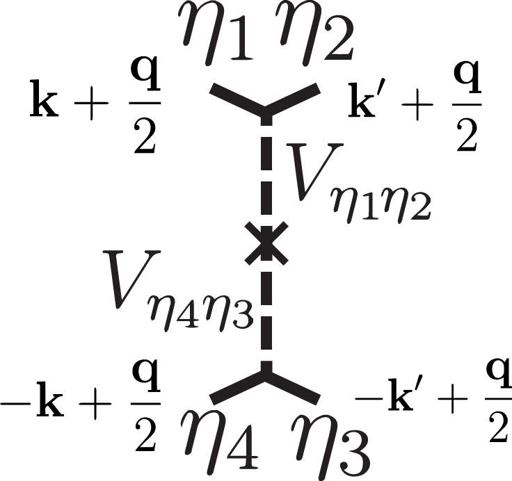
Figure 6: Diagrammatic presentation of the disorder scattering vertex, Eq. (B). The matrix elements $V_{\eta_{i}\eta_{j}}$ are given by Eq. (B).

The disorder scattering amplitude is schematically shown in Fig. 6. Based on Eqs.  (B) and (B) it takes the form,

$${}^{\eta_{1}}_{\eta_{4}}\!{\tilde{V}}^{\eta_{2}}_{\eta_{3}}\left(\mathbf{k},\mathbf{k}^{\prime};\mathbf{q,\mathbf{B}}\right)= V_{\eta_{1}\eta_{2}}\left(\mathbf{k},\mathbf{k}^{\prime};\mathbf{q},\mathbf{B}\right)$$

$$\times V_{\eta_{4}\eta_{3}}\left(-\mathbf{k},-\mathbf{k}^{\prime};\mathbf{q},\mathbf{B}\right).$$ (72)

To zero order in $q/k_{F}$ and $B/\Delta_{\mathrm{SO}}$, Eq. (B) simplifies,

$$V_{\eta\eta^{\prime}}\left(\varphi,\varphi^{\prime}\right)=\frac{V}{2}\left[1+\eta\eta^{\prime}e^{-i\left(\varphi-\varphi^{\prime}\right)}\right]\,.$$ (73)

The same limit of Eq. (73) turns Eq. (B) into Eq. (IV.2) of the main text.

Appendix C The contribution of the inter-band Cooper pairs

In this section we show that the contribution of the terms with $\eta\neq\eta^{\prime}$ to the integral equation (IV.2) is negligible in the range of parameters specified by Eq. (4). To this end we compute $\overline{\mathbb{G}}_{+}^{-}$ setting $\nu_{+}=\nu_{-}=\nu_{0}$, i.e. we set $x=0$. Using the definition, Eq. (41) the simple calculation gives ($\varepsilon_{n}>0$)

$$\overline{\mathbb{G}}^{+}_{-}\left(\varphi,\mathbf{q},\mathbf{B},\varepsilon_{n}\right)\!\approx\!\frac{2\pi\nu_{0}}{2\varepsilon_{n}+\Delta_{\mathrm{SO}}+iv_{F}(q_{x}+q_{y})+\frac{1}{\tau}}.$$ (74)

In contrast to Eq. (IV.2), Eq. (74) does not contain the field $\mathbf{B}$. Therefore at lease in the limit $x=0$ it contributes nothing both to the Lifhsitz invariant and to the PHE. The field dependence might appear in Eq. (74) at higher orders in $x$. This ensures that the contribution of inter-band processes to PHE is negligible. The same is true for the Lifshitz invariant since Eq. (74) contains an additional parameter, $\max\{T_{c},1/\tau\}/\Delta_{\mathrm{SO}}$ that is small in the regime, Eq. (4). We conclude that the contributions of the inter-band Cooper pairs are negligible in the regime, Eq. (4).

References

- Goldberg and Davis [1954] C. Goldberg and R. E. Davis, New galvanomagnetic effect, Phys. Rev. 94, 1121 (1954).
- Zhong et al. [2023] J. Zhong, J. Zhuang, and Y. Du, Recent progress on the planar hall effect in quantum materials, Chinese Physics B 32, 047203 (2023).
- Annadi et al. [2013] A. Annadi, Z. Huang, K. Gopinadhan, X. R. Wang, A. Srivastava, Z. Q. Liu, H. H. Ma, T. P. Sarkar, T. Venkatesan, and Ariando, Fourfold oscillation in anisotropic magnetoresistance and planar hall effect at the laalo3/srtio3 heterointerfaces: Effect of carrier confinement and electric field on magnetic interactions, Phys. Rev. B 87, 201102 (2013).
- Rout et al. [2017] P. K. Rout, I. Agireen, E. Maniv, M. Goldstein, and Y. Dagan, Six-fold crystalline anisotropic magnetoresistance in the (111) LaAlO3/SrTiO3 oxide interface, Phys. Rev. B 95, 241107 (2017).
- Maniv et al. [2017] E. Maniv, Y. Dagan, and M. Goldstein, Correlation-induced band competition in srtio3/laalo3, MRS Advances 2, 1243 (2017).
- Wadehra et al. [2020] N. Wadehra, R. Tomar, R. M. Varma, R. K. Gopal, Y. Singh, S. Dattagupta, and S. Chakraverty, Planar hall effect and anisotropic magnetoresistance in polar-polar interface of lavo3-ktao3 with strong spin-orbit coupling, Nature Communications 11, 874 (2020).
- Sulaev et al. [2015] A. Sulaev, M. Zeng, S.-Q. Shen, S. K. Cho, W. G. Zhu, Y. P. Feng, S. V. Eremeev, Y. Kawazoe, L. Shen, and L. Wang, Electrically tunable in-plane anisotropic magnetoresistance in topological insulator bisbtese2 nanodevices, Nano Letters 15, 2061 (2015).
- Taskin et al. [2017] A. A. Taskin, H. F. Legg, F. Yang, S. Sasaki, Y. Kanai, K. Matsumoto, A. Rosch, and Y. Ando, Planar hall effect from the surface of topological insulators, Nature Communications 8, 1340 (2017).
- Chiba et al. [2017] T. Chiba, S. Takahashi, and G. E. W. Bauer, Magnetic-proximity-induced magnetoresistance on topological insulators, Phys. Rev. B 95, 094428 (2017).
- Mehraeen and Zhang [2023] M. Mehraeen and S. S. L. Zhang, Proximity-induced nonlinear magnetoresistances on topological insulators (2023), arXiv:2312.05035 [cond-mat.mes-hall] .
- Akouala et al. [2019] C. R. Akouala, R. Kumar, S. Punugupati, C. L. Reynolds, J. G. Reynolds, E. J. Mily, J.-P. Maria, J. Narayan, and F. Hunte, Planar hall effect and anisotropic magnetoresistance in semiconducting and conducting oxide thin films, Applied Physics A 125, 293 (2019).
- Li et al. [2022] J. Li, Z. Wu, and G. Feng, Observation of planar hall effect in a strong spin-orbit coupling superconductor lao0.5f0.5bise2, Journal of Superconductivity and Novel Magnetism 35, 3521 (2022).
- Li et al. [2023] L. Li, E. Yi, B. Wang, G. Yu, B. Shen, Z. Yan, and M. Wang, Higher-order oscillatory planar hall effect in topological kagome metal, npj Quantum Materials 8, 2 (2023).
- Medel Onofre and Martín-Ruiz [2023] L. Medel Onofre and A. Martín-Ruiz, Planar hall effect in weyl semimetals induced by pseudoelectromagnetic fields, Phys. Rev. B 108, 155132 (2023).
- Bodnar et al. [2018] S. Y. Bodnar, L. Šmejkal, I. Turek, T. Jungwirth, O. Gomonay, J. Sinova, A. A. Sapozhnik, H. J. Elmers, M. Kläui, and M. Jourdan, Writing and reading antiferromagnetic mn2au by néel spin-orbit torques and large anisotropic magnetoresistance, Nature Communications 9, 348 (2018).
- Baltz et al. [2018] V. Baltz, A. Manchon, M. Tsoi, T. Moriyama, T. Ono, and Y. Tserkovnyak, Antiferromagnetic spintronics, Rev. Mod. Phys. 90, 015005 (2018).
- Yin et al. [2019] G. Yin, J.-X. Yu, Y. Liu, R. K. Lake, J. Zang, and K. L. Wang, Planar hall effect in antiferromagnetic mnte thin films, Phys. Rev. Lett. 122, 106602 (2019).
- Hamill et al. [2021] A. Hamill, B. Heischmidt, E. Sohn, D. Shaffer, K.-T. Tsai, X. Zhang, X. Xi, A. Suslov, H. Berger, L. Forró, F. J. Burnell, J. Shan, K. F. Mak, R. M. Fernandes, K. Wang, and V. S. Pribiag, Two-fold symmetric superconductivity in few-layer NbSe2, Nature Physics 17, 949 (2021).
- Cho et al. [2022] C.-w. Cho, J. Lyu, L. An, T. Han, K. T. Lo, C. Y. Ng, J. Hu, Y. Gao, G. Li, M. Huang, N. Wang, J. Schmalian, and R. Lortz, Nodal and nematic superconducting phases in NbSe2 monolayers from competing superconducting channels, Phys. Rev. Lett. 129, 087002 (2022).
- Smidman et al. [2017] M. Smidman, M. B. Salamon, H. Q. Yuan, and D. F. Agterberg, Superconductivity and spin–orbit coupling in non-centrosymmetric materials: a review, Reports on Progress in Physics 80, 036501 (2017).
- Sinova et al. [2004] J. Sinova, D. Culcer, Q. Niu, N. A. Sinitsyn, T. Jungwirth, and A. H. MacDonald, Universal intrinsic spin hall effect, Phys. Rev. Lett. 92, 126603 (2004).
- Schwab and Raimondi [2002] P. Schwab and R. Raimondi, Magnetoconductance of a two-dimensional metal in the presence of spin-orbit coupling, The European Physical Journal B - Condensed Matter and Complex Systems 25, 483 (2002).
- Inoue et al. [2004] J.-i. Inoue, G. E. W. Bauer, and L. W. Molenkamp, Suppression of the persistent spin hall current by defect scattering, Phys. Rev. B 70, 041303 (2004).
- Rashba [2004] E. I. Rashba, Sum rules for spin hall conductivity cancellation, Phys. Rev. B 70, 201309 (2004).
- Raimondi and Schwab [2005] R. Raimondi and P. Schwab, Spin-hall effect in a disordered two-dimensional electron system, Phys. Rev. B 71, 033311 (2005).
- Sinova et al. [2015] J. Sinova, S. O. Valenzuela, J. Wunderlich, C. H. Back, and T. Jungwirth, Spin hall effects, Rev. Mod. Phys. 87, 1213 (2015).
- Trushin et al. [2009] M. Trushin, K. Výborný, P. Moraczewski, A. A. Kovalev, J. Schliemann, and T. Jungwirth, Anisotropic magnetoresistance of spin-orbit coupled carriers scattered from polarized magnetic impurities, Phys. Rev. B 80, 134405 (2009).
- Zheng et al. [2020] S.-H. Zheng, H.-J. Duan, J.-K. Wang, J.-Y. Li, M.-X. Deng, and R.-Q. Wang, Origin of planar hall effect on the surface of topological insulators: Tilt of dirac cone by an in-plane magnetic field, Phys. Rev. B 101, 041408 (2020).
- Edelstein [1996] V. M. Edelstein, The ginzburg - landau equation for superconductors of polar symmetry, Journal of Physics: Condensed Matter 8, 339 (1996).
- Kochan et al. [2023] D. Kochan, A. Costa, I. Zhumagulov, and I. utić, Phenomenological theory of the supercurrent diode effect: The lifshitz invariant (2023), arXiv:2303.11975 [cond-mat.supr-con] .
- Gor’kov and Rashba [2001] L. P. Gor’kov and E. I. Rashba, Superconducting 2d system with lifted spin degeneracy: Mixed singlet-triplet state, Phys. Rev. Lett. 87, 037004 (2001).
- Frigeri et al. [2004] P. A. Frigeri, D. F. Agterberg, A. Koga, and M. Sigrist, Superconductivity without inversion symmetry: MnSi versus CePt3Si, Phys. Rev. Lett. 92, 097001 (2004).
- Yip [2014] S. Yip, Noncentrosymmetric superconductors, Annual Review of Condensed Matter Physics 5, 15 (2014), https://doi.org/10.1146/annurev-conmatphys-031113-133912 .
- Möckli and Khodas [2019] D. Möckli and M. Khodas, Magnetic-field induced pairing in ising superconductors, Phys. Rev. B 99, 180505 (2019).
- Larkin and Varlamov [2005] A. Larkin and A. Varlamov, Theory of Fluctuations in Superconductors (Oxford University Press, Incorporated, Oxford, UNITED KINGDOM, 2005) pp. –.
- Agterberg [2003] D. Agterberg, Novel magnetic field effects in unconventional superconductors, Physica C: Superconductivity 387, 13 (2003), proceedings of the 3rd Polish-US Workshop on Superconductivity and Magnetism of Advanced Materials.
- Hasan et al. [2022] J. Hasan, K. N. Nesterov, S. Li, M. Houzet, J. S. Meyer, and A. Levchenko, Anomalous Josephson effect in planar noncentrosymmetric superconducting devices, Phys. Rev. B 106, 214518 (2022).
- Houzet and Meyer [2015] M. Houzet and J. S. Meyer, Quasiclassical theory of disordered rashba superconductors, Phys. Rev. B 92, 014509 (2015).
- Möckli and Ramires [2021] D. Möckli and A. Ramires, Superconductivity in disordered locally noncentrosymmetric materials: An application to , Phys. Rev. B 104, 134517 (2021).
- Barzykin and Gor’kov [2002] V. Barzykin and L. P. Gor’kov, Inhomogeneous stripe phase revisited for surface superconductivity, Phys. Rev. Lett. 89, 227002 (2002).
- Bulaevskii et al. [1976] L. Bulaevskii, A. Guseinov, and A. Rusinov, Superconductivity in crystals without symmetry centers, Zh. Eksp. Teor. Fiz. 71, 2356 (1976).
- Ilić et al. [2017] S. Ilić, J. S. Meyer, and M. Houzet, Enhancement of the Upper Critical Field in Disordered Transition Metal Dichalcogenide Monolayers, Physical Review Letters 119, 117001 (2017).
- Edelstein [2021] V. M. Edelstein, Ginzburg-landau theory for impure superconductors of polar symmetry, Phys. Rev. B 103, 094507 (2021).
- Kopnin [2001] N. Kopnin, Theory of Nonequilibrium Superconductivity (Oxford University Press, 2001).