PULASki: Learning inter-rater variability using statistical distances to improve probabilistic segmentation

Abstract

In the domain of medical imaging, many supervised learning based methods for segmentation face several challenges such as high variability in annotations from multiple experts, paucity of labelled data and class imbalanced datasets. These issues may result in segmentations that lack the requisite precision for clinical analysis and can be misleadingly overconfident without associated uncertainty quantification. We propose the PULASki as a computationally efficient generative tool for biomedical image segmentation that accurately captures variability in expert annotations, even in small datasets. Our approach makes use of an improved loss function based on statistical distances in a conditional variational autoencoder structure (Probabilistic UNet), which improves learning of the conditional decoder compared to the standard cross-entropy particularly in class imbalanced problems. We analyse our method for two structurally different segmentation tasks ( intracranial vessel and multiple sclerosis (MS) lesion) and compare our results to four well-established baselines in terms of quantitative metrics and qualitative output. These experiments are characterised by class-imbalanced, low signal to noise ratio data sets with highly ambiguous features. Empirical results demonstrate the PULASKi method outperforms all baselines at the 5% significance level. Our experiments are also of the first to present a comparative study of the computationally feasible segmentation of complex geometries using 3D patches and the traditional use of 2D slices. The generated segmentations are shown to be much more anatomically plausible than in the 2D case, particularly for the vessel task. Our method can also be applied to a wide range of multi-label segmentation tasks and and is useful for downstream tasks such as hemodynamic modelling (computational fluid dynamics and data assimilation), clinical decision making, and treatment planning.

1 Introduction

The recent explosion in deep learning based medical image segmentation techniques has led to a dramatic improvement in the rapid diagnosis, treatment planning and modelling of various diseases [1, 2]. Medical image segmentation has specific challenges compared to other classical computer vision tasks, which has spurred the development of several bespoke machine learning tools [3, 4, 5]. Such issues include 1) limited availability of labelled training data, due to the expertise and excessive time required to create annotations; 2) class imbalance, particularly where the class of interest (e.g., tumour) is infrequently represented in the dataset; 3) complex and ambiguous features which are difficult to identify from Magnetic Resonance Imaging (MRI) data with low signal to noise ratio, leading to variation in annotations from different graders for the same image; and 4) considerable anatomic variability between patients. As a result, quantifying the uncertainty in predicted segmentations, regardless of the chosen method, is paramount to prevent over-confident and biased diagnoses [6, 7]. Generating multiple plausible segmentations also supports ensemble-based uncertainty quantification in biomedical computational fluid dynamics (CFD) models (e.g., [8, 9]). We propose an accurate and computationally feasible method for generating ensembles of plausible segmentations in medical applications plagued by the aforementioned issues.

Significant research effort in the field of deep learning based medical image segmentation has focused on improving the accuracy of convolutional neural networks (CNNs). By now, the U-Net [10] and Attention U-Net [11] have emerged as empirically successful methods for image segmentation in a range of computer vision tasks not limited to medical imaginEnhancements of such methods have been developed to remain competitive when trained on small data sets, e.g., via deformation consistent, multiscale supervision [12], along with improved loss functions for heavily class imbalanced data sets, such as the Focal Tversky Loss [13]. However, uncertainty quantification of such outputs remains a considerable challenge, which is exacerbated when training data are sparse. Furthermore, the logits or activations produced from most deep learning based segmentation methods provide only a pixel-wise measure of uncertainty and cannot be reliably used to generate samples from the underlying joint distribution [14, 15]. This necessitates tailor-made methods that carefully account for the joint probability between pixels, as in, for instance, Deep Ensembles [16] and Stochastic Segmentation Networks [14].

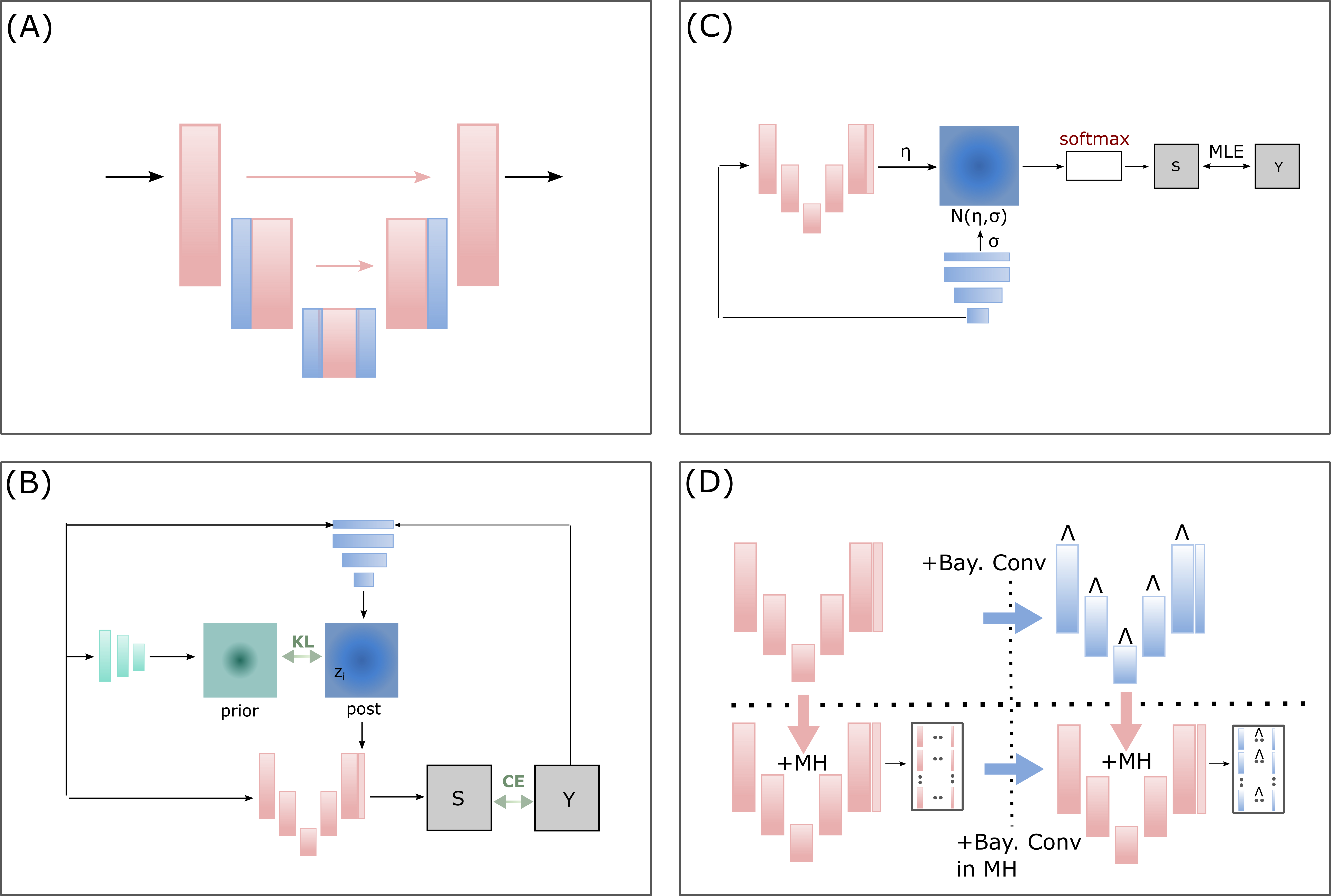
While Bayesian methods [17, 18, 19] are supported by rich theory for quantifying both aleatoric and epistemic uncertainty, it is necessary to resort to approximations of both the prior and posterior in most high dimensional medical imaging applications. In Bayesian neural networks, weights are treated as random variables whose distributional properties must also be estimated from data. This is particularly challenging in medical imaging problems where annotated data sets are limited, thus exacerbating the issue of parameter identifiability [20]. Arguably the most prominent, flexible and easily implementable approach is Monte Carlo dropout [21, 22], which involves randomly removing elements of the input tensor [23] or removing channels (i.e., feature maps) while using spatial dropouts with convolutional layers [24], during both training and inference. This serves as a fast but somewhat crude approximation to the posterior. Variational autoencoder and variational inference methods, such as the Probabilistic U-Net [25], Variational Inference U-Net (VI U-Net) and Multi-Head VI U-Net [26]) can serve as a fast and reasonably approximation, as they not only drastically simplify computation of the posterior, but typically also capture uncertainty through a lower dimensional latent variable which is more identifiable. However, these methods rely on a cross-entropy style reconstruction term in the evidence lower bound (ELBO), which is known to be problematic for class imbalanced data sets [13, 27, 28], as is common in medical image segmentation.

A modified version of the Probabilistic U-net [25] that allows for improved representation of inter-rater variability in annotations in class-imbalanced data has been investigated in this research, by experimenting with a range of distribution losses. The literature lacks 3D implementation of generative models, whereas a comparison between 2D and 3D models is rarely performed. Hence, this research also investigates the influence of training on 2D slices compared to 3D patchesTesting of the method is primarily focused on intracranial segmentations of blood vessels and lesions due to multiple sclerosis. The features of interest are complex in their geometry and ambiguous and there exists appreciable variability in annotations between graders. We focus on methods capable of generating ensembles of segmentations that can then be used to represent uncertainty in the model domain in hemodynamic models. These models are crucial for better understanding the development and diagnoses of cardiovascular and neurovascular diseases which count as the 1st and 2nd leading cause of death worldwide [29, 30, 9]. Although we verify our method on intracranial segmentation, it can be applied to other segmentation tasks where multiple annotations per image are available.

2 Background

Figure 1: Schematic of Baseline Methods: (A): Monte-Carlo-Dropout (MC-DO); (B): Probabilistic U-Net (ProbU-Net); (C): Stochastic Segmentation Network (SSN); (D): Multi-head Variational Inference U-Net (MH VI U-Net)

2.1 Notation

Throughout the manuscript, we make use of the following notation:

• $x=$ random variable representing image data, i.e. a 2D or 3D matrix containing brightness values for each pixel/voxel.

• ${\bf x}=$ dataset consisting of $N$ independent and identically distributed data of the random variable $x$.

• $x_{ijk}$ = entry in the $i$th position of the first dimension (i.e. row), $j$th position of the second dimension (i.e. column) and $k$th position of the third dimension of a 3D matrix $x$.

• $y$ = random variable denoting the “ground truth” segmentation of the image $x$.

• $c_{ij}$ = categorical random variable of the class for the $ij$th pixel

• $s=$ predicted plausible segmentation for an image $x$, with the same dimensions as $x$.

• $\{v^{i}\}_{i=1:M}$ denotes a set of $M$ plausible samples of a random variable $v$.

• $z\in\mathbb{R}^{p}=$ $p$-channel feature map of image-segmentation pair.

• $\eta$ = logits i.e. outputs from the final activation layer of a given neural network. When $x$ is a 2D image of size $d\times d$, $\eta\in\mathbb{R}^{d\times d\times K}$ where $K$ is the desired number of classes.

• $M$ = number of samples from posterior net or no. of plausible segmentations per image.

Finally, we use ${}^{\prime}.^{\prime}$ to indicate the multiplication operation and reserve use of $\times$ when defining sizes of matrices.

2.2 U-Net

The U-Net [10] is a CNN characterised by a contracting network comprising successive convolution, ReLU activation and max-pooling layers that generates low resolution feature maps, combined with an expanding network where max-pooling is replaced by upsampling to increase the resolution of the output. Skip connections allow high resolution features generated along the contracting network to be combined with the upsampling output, thereby improving the precision of the segmentation. We summarise the U-Net architecture using the following simplified notation

$$\tilde{x} =f_{U}(x;\psi_{u});\quad\tilde{x}\in\mathbb{R}^{d\times d\times 64}$$ (1)

$$\eta =f_{1\times 1}(\tilde{x},\psi_{1});\quad\eta\in\mathbb{R}^{d\times d\times K}$$ (2)

where the input $x\in\mathbb{R}^{d\times d}$ represents a 2D matrix of pixel values (but can also accommodate 3D images); $f_{U}$ denotes the combination of all $3\times 3$ convolution, ReLU, pooling and up-convolution layers in the U-Net; $\tilde{x}\in\mathbb{R}^{d\times d\times 64}$ is a 64-channel feature map of the same resolution as the input image; $f_{1\times 1}$ is a $1\times 1$ convolution layer that reduces the dimensionality of the feature space to that of the desired number of classes, $K$; $\eta\in\mathbb{R}^{d\times d\times K}$ is a $K$-channel feature map of the same resolution as the original image; and $\psi=[\psi_{u},\psi_{1}]$ is a vector of trainable parameters (e.g., convolution kernel weights). The categorical distribution of $c_{ij}$, the class for the $ij$th pixel, is then obtained by converting the feature map $\eta$ to a probability for each channel or class using the soft-max operator, i.e.

$$p_{\eta}\left(c_{ij}=k\right)=\frac{\exp\left(\eta_{ijk}\right)}{\sum_{k=1}^{K}\exp\left(\eta_{ijk}\right)}$$ (3)

Since we are primarily interested in binary segmentation ($K=2$), we consider a special case of the soft-max operator, the sigmoid function, to compute class probabilities,

$$p_{\eta}(c_{ij}=1) =\frac{1}{1+\exp(-\beta_{ij})},$$ (4)

$$p_{\eta}(c_{ij}=0) =1-p_{\eta}(c_{ij}=1)=\frac{\exp(-\beta_{ij})}{1+\exp(-\beta_{ij})}.$$ (5)

where $\beta_{i,j}:=\eta_{ij1}-\eta_{ij0}$. Finally, the predicted segmentation $s$, is given by a $d\times d$ integer-valued matrix of class labels from the set $\{1,2,\cdots,K\}$, where $s_{ij}$ is typically obtained by selecting the label corresponding to the maximum class probability,

$$s_{ij} =\arg\max_{k}p_{k}\left(\eta_{ij}\right),\quad\text{for all}\enskip i,j.$$ (6)

This approach is known to produce unrealistic and noisy segmentations [31], hence we adopt a commonly used image thresholding strategy suitable for binary segmentation whereby

$$s_{ij}=\begin{cases}1&p_{\eta}(c_{ij}=1)\geq\tau\\ 0&\text{otherwise},\end{cases}$$ (7)

where $\tau$ is decision threshold. This threshold is determined using Otsu’s method [32] which gives the optimal value of $\tau$ that minimises intra-class intensity variance. Note that $\tau=0.5$ corresponds to (6).

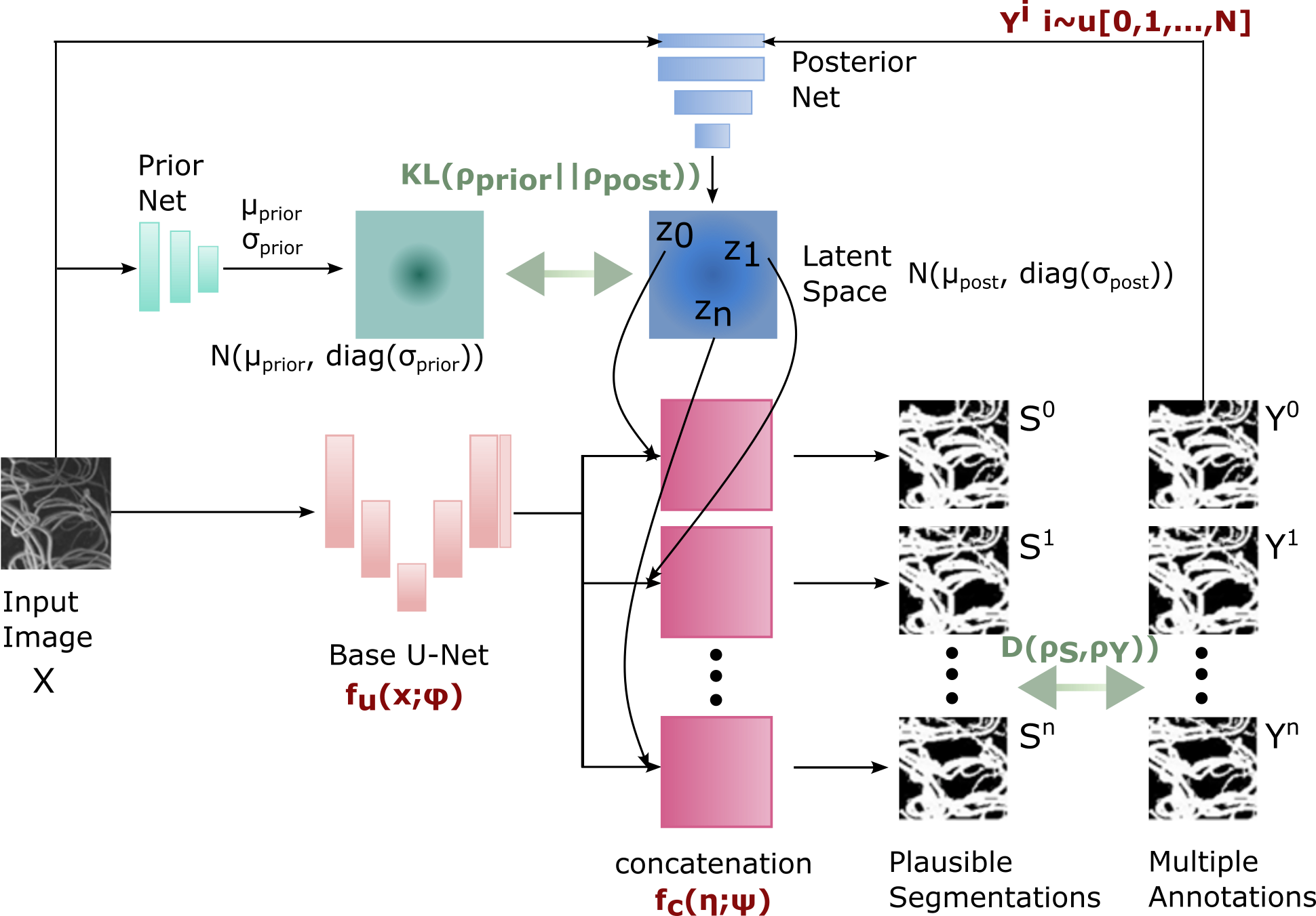
2.3 Probabilistic U-Net

The U-Net in principle provides probabilistic outputs through independent pixel-wise categorical distributions (see 3), although it provides a poor representation of the dependence between pixels. The Probabilistic U-Net [25] has emerged as an empirically competitive approach to quantifying aleatoric uncertainty by making use of ideas from conditional variational auto-encoders (cVAEs) and $\beta$-VAEs [33, 34]. This is done by incorporating a random latent factor $z\in\mathbb{R}^{d}$, that represents a low dimensional embedding of the image-segmentation pair, which is then used to efficiently generate samples of plausible segmentations $s$. The distribution of $z$ is captured through the intractable posterior $p_{\theta}(z|{\bf x,y})$, whose form is learned from the data. In cVAEs, the goal is to determine $\theta,\phi$ such that a more tractable form $q_{\phi}(z|{\bf x,y})$ best approximates the intractable posterior $p_{\theta}(z|{\bf x},{\bf y})$ and $p_{\theta}(x|{\bf y})$ approximates the true conditional data distribution $p(x|{\bf y})$. As is common in many applications of variational inference, the posterior $p_{\theta}(z|{\bf x,y})$ is assumed to be well approximated by a Gaussian distribution,

$$q_{\phi}(z|{\bf x},{\bf y})=N(\mu({\bf x},{\bf y}),\Sigma({\bf x},{\bf y})),$$ (8)

where $\mu({\bf x},{\bf y})\in\mathbb{R}^{d}$, $\Sigma({\bf x},{\bf y})$ a $d\times d$ matrix with zeros on the off-diagonal and diagonal given by $\sigma({\bf x},{\bf y})\in\mathbb{R}^{d}$. The mean and covariance $\mu$ and $\sigma$ respectively are given by,

$$\mu(x,y)=NN_{post,\mu}\left(x,y;\phi_{\mu}\right),$$ (9)

$$\sigma(x,y)=NN_{post,\sigma}\left(x,y;\phi_{\sigma}\right),$$

where $NN_{post,\mu}(x,y;\phi_{\mu})$ indicates a neural network that takes as input an image $x$ and its corresponding segmentation $y$ and is parameterised by $\phi_{\mu}$; and $\phi=[\phi_{\mu},\phi_{\sigma}]$. The parameters $\theta,\phi$ are determined by minimising a modified version of the per-datapoint negative evidence lower bound (ELBO), given by

$$\underbrace{-\mathbb{E}_{q_{\phi}(z|x,y)}[\log p_{\theta}(y|x,z)]}_{\text{reconstruction term}}+\beta\underbrace{KL(q_{\phi}(z|x,y)||p_{\theta}(z|x))}_{\text{regularisation term}},$$ (10)

where $\beta$ is a tuning parameter controlling the influence of the regularisation term and $p_{\theta}({\bf z}|{\bf x})$ is the conditional prior on $z$ which is also learnt from the data. It takes a similar form to the approximate posterior except that only images ${\bf x}$ are taken as inputs, i.e. $p_{\theta}(z|{\bf x})=N(\mu_{prior}({\bf x}),\Sigma_{prior}({\bf x}))$, with

$$\mu_{\text{prior }}(x)=NN_{\text{prior},\mu}\left(x;\theta_{\mu}\right)$$ (11)

$$\sigma_{\text{prior }}(x)=NN_{\text{prior },\sigma}\left(x;\theta_{\sigma}\right),$$

and $\theta=[\theta_{\mu},\theta_{\sigma}]$ denotes the weights and biases of the prior neural networks. The reconstruction term in 10 is equivalent to the expected cross-entropy, which penalises differences between the ground truth segmentation $y$ and generated segmentation $s$. In summary, the entire set of parameters $\{\theta,\psi,\phi\}$ is jointly learned by minimising an empirical approximation of the loss function 10 assuming independent and identically distributed (iid) data, given by

$$\sum_{n=1}^{N}\left(\frac{1}{M}\sum_{m=1}^{M}-\log p_{\eta^{m,n}}(c=y^{n})\right)+\beta KL(q_{\phi}(z|x^{n},y^{n})||p_{\theta}(z|x^{n}))$$ (12)

where $p_{\eta^{m,n}}(c=y^{n})=\prod_{ij}p_{\eta^{m,n}}(c_{ij}=y_{ij}^{n})$ and $p_{\eta^{m,n}}(c_{ij}=y^{n}_{ij})$ is the class probability of the $i,j$th pixel corresponding to the $n$th true segmentation $y^{n}$, computed using the softmax or sigmoid operator (3 or 4-5 respectively). The feature map corresponding to the $n$th image is obtained using a minor modification to the standard U-Net,

$$\tilde{x}^{n} =f_{U}(x^{n};\psi_{u});$$ (13)

$$z^{m,n} \sim q_{\phi}(z|x^{n},y^{n});$$ (14)

$$\eta^{m,n} =[f_{1\times 1}(\tilde{x}^{n},\psi_{1});E_{d\times d}(z^{m,n})]$$ (15)

where $E_{d\times d}$ denotes the expansion operation that expands $z^{n}$ by repeating its values to match the dimensions of $f_{1\times 1}(\tilde{x}^{n},\psi_{1})$. Further details on training are given in Section 4.3. Once trained, a set of $M$ plausible segmentations for a new image $\mathcal{X}$ can be obtained by evaluating 13-15 $M$ times with 14 replaced by

$$z^{i} \sim p_{\theta}(z|\mathcal{X})$$ (16)

The resulting feature map for each sample is then converted to a segmentation using the same procedure as detailed in section 2.2. An overview of the method can be found in Figure 1b.

2.4 Multi-head Variational Inference U-Net (MH VI U-Net)

The MH-VI U-Net [26] is a variational inference based extension of the multi-headed U-Netwhich aims to improve out-of-distribution robustness. The multi-head approach consists of a base model (e.g., a U-Net) and an ensemble of “heads”, typically a series of convolutions in the final layers of the U-Net. The MH-VI U-Net aims to improve on the classical MH U-Net by replacing regular convolutions with Bayesian convolutions in the heads. The classical MH U-Net allows only for maximum likelihood estimation of the weights at each head.

The base model is taken to be a reduced parameter version of the U-Net, and the depth of each head is typically restricted by the number of heads due to memory constraints. Variational inference is then employed to efficiently approximate the posterior distribution of the weights in head $h$, $w_{h}$ which is approximated by $q_{\theta_{h}}(w_{h})$. Here $\Theta=[\theta_{1},\theta_{2},\cdots,\theta_{H}]$ denotes the variational parameters to be optimised, obtained by minimising a linear combination of the per head negative ELBO and the joint ELBO over all $H$ heads given by

$$\lambda\mathcal{L}_{\Theta}({\bf x,y})+(1-\lambda)\frac{1}{H}\sum_{h=1}^{H}\mathcal{L}_{\theta_{h}}({\bf x,y})$$ (17)

where $\mathcal{L}_{\mu}({\bf x,y})$ is the negative ELBO, i.e.

$$\mathcal{L}_{\mu}({\bf x,y}):=-\mathbb{E}_{q_{\mu}(w)}[\log p({\bf y}|{\bf x},w)]+\beta KL(q_{\mu}(w)||p(w))$$ (18)

where $\beta$ is the temperature, $w$ is a vector of the weights of the U-Net and $\mu$ denotes the variational parameters to be optimised. The tuning parameter $\lambda$ can be seen as a bridge between classical deep ensemble training $(\lambda=0)$ and joint estimation $(\lambda=1)$. While both the VI-MH U-Net and the Probabilistic U-Net rely on variational inference, they primarily differ in terms of how randomness is introduced into the U-Net: in the VI-MH U-Net this is via the weights of the network, compared to in the probabilistic U-Net where this is done on some low dimensional latent feature map.

2.5 Stochastic Segmentation Networks (SSN)

Stochastic Segmentation Networks [14] were proposed to model aleatoric uncertainty primarily due to integrader variability. Unlike the Probabilistic U-Net, the SSN can be more easily used with any neural network based segmentation model. The logits (i.e. inputs to the softmax) $\eta\in\mathbb{R}^{d^{2}.K\times 1}$, represented here as a flattened vector, are modelled as a Gaussian random variable whose mean and covariance are modelled by neural networks,

$$p_{\gamma}(\eta|x)=N(\mu(x),\Sigma(x)),$$ (19)

where

$$\Sigma(x)=PP^{T}+D,$$ (20)

and $P\in\mathbb{R}^{d^{2}.K\times R}$ is known as a covariance factor and $R$ controls the rank of the matrix and $D\in\mathbb{R}^{d^{2}K\times d^{2}K}$ is a diagonal matrix with $\sigma$ on the diagonal. The mean, covariance factor and diagonal are represented by neural networks,

$$\mu(x) =NN_{\mu}(x;\gamma_{\mu})$$ (21)

$$\sigma(x) =NN_{\sigma}(x;\gamma_{\sigma})$$

$$P(x) =NN_{P}(x;\gamma_{P}).$$

where the parameters $\gamma=[\gamma_{\mu},\gamma_{\sigma},\gamma_{P}]$ are learnt during training. Note that unlike in the Probabilistic U-Net, the uncertainty on the logits is not updated according to the segmentation masks $y$ in the training data, in other words, there is no Bayesian updating of a prior to a posterior. The parameters of the segmentation network, $\psi$, and $\gamma$ are jointly learned by minimising the negative log-likelihood over the entire dataset, assuming iid data,

$$-\log\left(p({\bf y}|{\bf x})\right) =-\sum_{n=1}^{n}\log\left(\mathbb{E}_{p_{\gamma}(\eta^{n}|x^{n})}[p(y^{n}|\eta^{n})]\right)$$ (22)

$$\approx-\sum_{n=1}^{n}\log\left(\frac{1}{M}\sum_{m=1}^{M}\prod_{i,j}p_{\eta^{n,m}}(c_{ij}=y^{n}_{ij})\right)$$ (23)

where $\eta^{n,m}\sim N(\mu(x^{n}),\Sigma(x^{n}))$ as defined in 19. Note that 22 takes a similar form to 12 but without a regularisation term due to the lack of the Bayesian update. This may potentially lead to a less tractable optimisation problem that may have difficulty converging [35].

2.6 Monte Carlo Dropout

Monte Carlo Dropout (MCDO) is a widespread tool for approximating model uncertainty in neural networks by randomly removing layers during both training and prediction phases [36, 37]. In the context of the U-Net, MCDO can be implemented by adding spatial dropout layers [24] after every encoding (pair of convolution layers with batch normalisation and ReLU activations, followed by average pooling) and decoding block (transposed convolution, followed by a pair of convolution layers wit batch normalisation and ReLU). The key idea behind MCDO is to randomly switch on and off neurons (i.e. set their weights to zero) according to a pre-specified probability. Running this procedure $M$ times allows one to generate $M$ segmentations. However, it is noteworthy that even though utilising the Dropout function is computationally inexpensive, there are a number of intrinsic shortcomings of MCDO, such as unreliable uncertainty quantification, subpar calibration, and inadequate out-of-distribution detection [26].

3 PULASki - Probabilistic Unet Loss Assessed through Statistical distances

Figure 2: Schematic of the proposed PULASki method.

Our main focus is to improve the capability of U-Net based image segmentation methods to capture predicted aleatoric uncertainty, primarily due to inter-rater variability. Inter-rater variability is a persistent issue in biomedical segmentation which arises primarily due to the low signal to noise ratio in the raw data and complexity of the features being segmented (e.g., small cerebral vessels). In the original formulation of the Probabilistic U-Net, the reconstruction term in the ELBO 10 can be seen as an empirical approximation of the expected cross-entropy,

$$\mathbb{E}_{z\sim q_{\phi}(z|x,y)}[H(p(y|x),p_{\theta}(y|z,x)]$$ (24)

where

$$H(p(y|x),p_{\theta}(y|z,x))=-\sum_{y\in\mathcal{Y}}p(y|x)\log p_{\theta}(y|z,x)$$ (25)

and $\mathcal{Y}$ is the set of all possible segmentations for a given image. The standard cross-entropy has several known shortcomings for class-imbalanced datasets and for multi-label classification problems [13, 27, 28]. An empirical approximation of the cross-entropy between $p(y|x)$ and $p_{\theta}(y|z,x)$ when used to approximate the ELBO is indistinguishable from the standard ELBO (12) when multiple labels are treated as conditionally independent data. This makes it poorly suited for learning the conditional distribution $p(y|x)$.

We propose to modify the loss function 12 in the probabilistic U-Net by replacing the expected cross-entropy term with a more general statistical distance between $p_{\theta}(y|x)$ and $p(y|x)$. Various choices are possible, and we focus our attention on those that have the potential to more efficiently capture features of $p(y|x)$ when only samples from it are available. Our proposed loss function (per data point) is

$$\mathbb{E}_{z\sim q_{\phi}(z|x,y)}\left[D(p(y|x),p_{\theta}(y|x,z))\right]+\beta KL(q_{\phi}(z|x,y)||p_{\theta}(z|x))$$ (26)

where $D(p,q)$ is an appropriate statistical distance between two probability distributions $p,q$. In practice, distances are usually approximated using the empirical distributions; Samples from $p_{\theta}(y|x,z)$ can be easily generated during training using the same operations as for the Probabilistic U-Net (see 13 - 15. An empirical approximation of $p(y|x)$ is available whenever there are multiple plausible segmentations per image. A schematic of the method can be found in Figure 2. Our proposed method bears some resemblance to wasserstein autoencoders [38], although our primary focus is on varying the reconstruction loss for conditioned generation whereas their focus is on alternative regularisation terms.

Crucially, all statistical distances considered here are differentiable, so that they can be used as loss-functions in standard gradient-based optimisation methods such as ADAM. We focus on distances that are well known in the image analysis literature, as described below.

3.1 Frechet Inception Distance (FID)

The FID [39] is a pseudometric based on the Wasserstein-2 distance and is widely used particularly in training GANs for image generation. Computing the Wasserstein-2 distance between two arbitrary empirical distributions can be computationally prohibitive in DL applications which require repeated evaluations during training. Calculation of the FID requires approximating the distributions by a Gaussian, which then allows one to exploit the existence of a closed form solution to the Wasserstein-2 distance for Gaussian distributions, making it fast to implement. It provides a reasonable approximation for distributions whose first two moments exist, although it can produce biased estimates [40].

In the image generation or segmentation context, the FID is computed as

$$D_{FID}:=|\mu-\hat{\mu}|_{2}^{2}+Tr(\Sigma+\hat{\Sigma}-2(\Sigma^{1/2}\hat{\Sigma}\Sigma^{1/2})^{1/2})$$ (27)

where $\hat{\mu}\in\mathbb{R}^{v}$ and $\hat{\Sigma}\in\mathbb{R}^{v\times v}$ are the sample mean and covariance respectively of $\{a^{m}\}_{m=1:M}$ where $a^{m}$ denotes a flattened (i.e. vectorised) version of the matrix $\eta^{m}$ as defined in 15 of length $v=d\times d\times K$. Likewise, $\mu$ and $\Sigma$ denote the sample mean and covariance respectively of the final activations (i.e. logits) from an Inception Net V3 [41] which takes the plausible segmentations rather than raw images as inputs. Since the inception net is only trained on 2D images, we only make use of the FID for the experiments involving 2D images.

3.2 Hausdorff Divergence

The Hausdorff distance is a way of measuring distances between subsets of metric spaces (rather than measure spaces). It has traditionally been used in computer vision to measure the degree of similarity between two objects, such as image segmentations, by measuring distances between points of the two sets. The traditional Hausdorff distance can be lifted to measuring statistical distance between probability measures. In the case of discrete measures $\alpha,\beta$ on $\mathbb{R}^{d}$ given as weighted point clouds i.e.

$$\alpha=\sum_{i=1}^{N}\alpha_{i}\delta_{x_{i}};\quad\beta=\sum_{i=1}^{N}\beta_{i}\delta_{y_{i}};$$ (28)

where $\delta_{x}$ is the Dirac delta function centred at $x$, the Hausdorff divergence is defined (as per definition A.2 in [42]) as

$$d_{H}(\alpha,\beta):=\frac{1}{2}\langle\alpha-\beta,\nabla F_{\epsilon}(\alpha)-\nabla F_{\epsilon}(\beta)\rangle.$$ (29)

The Hausdorff divergence is equivalent to the symmetric Bregman divergence induced by $F_{\epsilon}$, a strictly convex functional, where $F_{\epsilon}$ is the Sinkhorn negentropy, defined as:

$$F_{\epsilon}(\alpha):=-\frac{1}{2}\mathrm{OT}_{\epsilon}(\alpha,\alpha)$$ (30)

where $OT_{\epsilon}$ is the entropy-regularised optimal transport cost, given by:

$$OT_{\epsilon}(\alpha,\beta)=\min_{\pi\in M^{+}(X\times X)}\left\langle\pi,C(x,y)\right\rangle+\epsilon KL(\pi||\alpha\otimes\beta)$$ (31)

and we let $C(x,y)=\frac{1}{2}\|x-y\|_{2}^{2}$,i.e. the squared Euclidean distance (corresponding to the Wasserstein-2 distance).

The above is more specifically referred to as the $\epsilon$-Hausdorff divergence, as it is based on $OT_{\epsilon}$ which only produces an $\epsilon$-approximate solution to the exact OT problem. The $\epsilon$-Hausdorff divergence is generally cheaper to compute than the closely related $\epsilon$-Sinkhorn divergence or debiased Sinkhorn divergence (see Section 3.3) as it relies on solving the symmetric OT problem $OT_{\epsilon}(\alpha,\alpha)$ rather than $OT_{\epsilon}(\alpha,\beta)$.

3.3 de-biased Sinkhorn divergence

A more accurate but computationally expensive approximation of the $p$-Wasserstein distance is the so-called de-biased Sinkhorn divergence [43]

$$S_{\epsilon}(\alpha,\beta):=\text{OT}_{\epsilon}(\alpha,\beta)-\frac{1}{2}\text{OT}_{\epsilon}(\alpha,\alpha)-\frac{1}{2}\text{OT}_{\epsilon}(\beta,\beta)$$ (32)

where $\alpha,\beta$ are any positive measures and $\text{OT}_{\epsilon}$ is the entropic-regularised form of the optimal transport loss 31. This divergence has been used in training generative models (See e.g. [44] ). We utilise the method proposed in [42] which makes use of a multiscale Sinkhorn algorithm to compute $S_{\epsilon}(\alpha,\beta)$.

4 Experiments

4.1 Datasets and Labels

Figure 3: Rate of occurrence (RoO) of labels across multiple annotations. The brighter (yellow) the voxel appears, the more often it is labelled as vessel (A) or lesion (B) across the available annotations. (A): Ten segmentations per image from one subject in OpenNeuro’s ‘StudyForrest’ dataset were generated using the Frangi filter. A vessel cross section at the location of the red line is displayed within the red square. (B): Multiple Sclerosis lesion segmentations from 7 expert annotators for one subject.

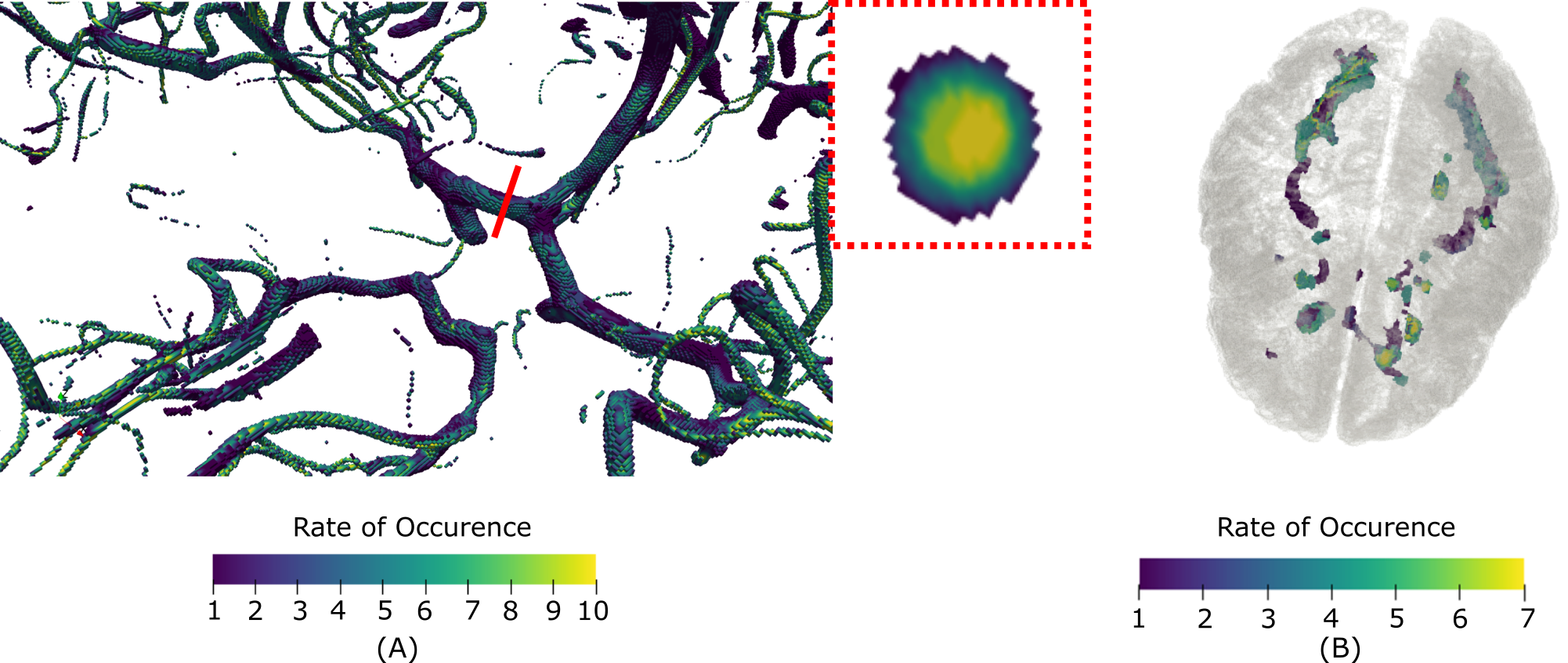
To be able to validate the proposed approach, the OpenNeuro’s ‘StudyForrest’ dataset which contains 20 subjects was used for vessel segmentation. It contains 7T MRA-ToF full brain volumetric images with [480 × 640 × 163] matrix size in NIFTI format recorded with a Siemens MR scanner at 7-Tesla using a 3D Multiple Overlapping Thin Slab Acquisition Time of Flight angiography sequence (0.3 mm isotropic voxel size) [45]. Training the network requires multiple plausible segmentations. For the ‘StudyForrest’ dataset, multiple manual labels did not exist. Therefore, ten synthetic plausible segmentations per case have been generated using the Frangi filter [46]. The Frangi scale range has been set to $\sigma$ $\sim$ [1 8] and a step size between the sigmas of 2 was chosen. Following parameters, known as vesselness constants, have been sampled from truncated normal distributions: (i) $\mathrm{Frangi}_{\alpha}$ $\sim$ TN(0.5 1) determines if its a line (vessel) or plane like structure; (ii) $\mathrm{Frangi}_{\beta}$ $\sim$ TN(0.5 1) determines the deviation from a blob like structure; (iii) $\mathrm{Frangi}_{C}$ $\sim$ TN(500 100) gives a threshold between eigenvalues of noise and vessel structures. The resulting ”inter-rater” agreement of the generated dataset was calculated using $K\alpha$ (discussed later in Sec. 4.3) and has a value of 0.40.

For further validating the proposed method, 3T FLAIR MRIs from the publicly available multiple sclerosis (MS) segmentation dataset, that was used for MICCAI 2016 challenge [47], containing MRI scans of 53 patients and their corresponding manual segmentations of the lesions by seven experts, was utilised. After thorough examination of expert voting, one subject was excluded due to significant discrepancies in expert annotations. In this case, two graders determined that no voxels represented an MS lesion, four experts identified only a few voxels as MS tissue, and one grader marked nearly the entire brain. Accurate identification of multiple sclerosis lesions is difficult due to variability in lesion location, size and shape – which is also reflected in the resulting very low inter-rater agreement. The inter-rater agreement was assessed using $K\alpha$ for the MS dataset, resulting in an agreement of 0.60. However, when considering only brain regions where at least one grader noted an MS occurrence, the alpha decreased to 0.28.

The Rate of Occurence (RoO), illustrating the frequency of a voxel being labeled as a vessel or MS lesion in the annotation is displayed in Figure 3. The RoO serves as a visual representation of the data variability, complementing the $K\alpha$ coefficient. The overall darker shade of the CoW region in the vessel image indicates high variability in the underlying plausible segmentations. The cross-sectional view of the vessel reveals that variability increases with distance from the center of the vessel. Smaller vessels exhibit comparatively lower variability, even in the outer regions, when compared with the larger vessels within the CoW region. In the MS dataset, certain expansive regions, denoted by dark blue areas, are identified as lesions by only one grader. Voxels at the center of the MS region are consistently marked as MS by (almost) all graders.

4.2 Implementation

There are two methods for managing 3D volumetric images: (i) processing them in 2D, treating each slice as an individual data point, or (ii) working directly in 3D. However, due to computational limitations, it is often impossible to work with the full 3D volume. Hence, patch-based approaches are adapted. These patches can be 3D patches (3D sub-blocks from the 3D volume), or 2D patches (2D slices taken a particular imaging plane). 2D models are less computationally hungry, while 3D patches provide better spatial context encoding possibility. This research explores both these directions – working with 2D slices following the acquisition plane using 2D models utilising 2D convolution operations and working with 3D patches employing 3D models with 3D convolution operations.

The PULASki method was implemented by extending the pipeline available from DS6 [12]. It is based on PyTorch [48] and used TorchIO [49] for creating 3D patches or extracting 2D slices from the available 3D volumes. All the statistical distances used in PULASKi (discussed in Sec. 3) were calculated using the GeomLoss [50]. The weights and biases of all the models (proposed and baselines, including their sub-models – e.g., prior net), were initialised by sampling a uniform distribution $\mathcal{U}(-\sqrt{k},\sqrt{k})$, where $k=\frac{\text{ groups }}{C_{\text{in }}*\prod_{i=0}^{1}\text{ kernel\_size }[i]}$ for the convolutional layers and $k=\frac{1}{in\_features}$ for the linear layers.

In this implementation, the latent space was formulated using three convolutional channels, each with a single pixel/voxel (shape 1x1 for 2D and 1x1x1 for 3D), resulting in the size of the latent variable being three. These channels were expanded to the original input size prior to ’injecting’ them into the last layer of the base U-Net of the probabilistic U-Nets (PULASki methods, as well as baseline Prob UNet). This ’injection’ is performed by concatenating a sampled value from the latent space with the output of the penultimate layer of the base U-Net, and then supplying it to the final layer, which is a convolutional layer with a kernel size of 1x1 or 1x1x1 for the 2D and 3D versions, respectively.

The baseline probabilistic U-Net experiments were performed by adapting the PyTorch implementation available from [51]. As the loss function for the baseline probabilistic UNet, as well as for the MCDO UNet, Focal Tversky Loss (FTL) [13] was employed. Cross-entropy (CE) loss used in the original probabilisitic UNet work was replaced with FTL as CE might not be optimal when there is a big imbalance between the positive (1) and negative (0) classes in the image mask as CE treats them both equally – a common scenario in medical image segmentation tasks [52, 28]. A balanced version of CE loss (weighted CE) might combat this issue [28]. Dice loss, on the other hand, is a commonly used loss function in medical image segmentation tasks, providing a better trade-off between precision and recall [13]. FTL, designed specifically for medical image segmentation tasks, achieves an even better trade-off between precision and recall when training on small structures [13], and has also been shown to outperform CE, weighted CE, and Dice [52].

The SSN method was performed using the DeepMedic convolutional neural network [53] as backbone, as was done in the original paper [14]. DeepMedic is a dual pathway, 11 layers deep, three-dimensional convolutional neural network, that was developed for brain lesion segmentation. The network has two parallel convolutional pathways that process the input images at multiple scales simultaneously, capturing both local and larger contextual information, and employs a novel training scheme that alleviates the class-imbalance problem and enables dense training on 3D image segments. Contrary to U-Nets, which condense and then expand the input to produce the final output, DeepMedic employs a fully convolutional network that processes the input at different resolutions through two parallel pathways, then uses a series of convolutional and pooling layers to extract features at different scales, and finally combines these features through concatenation and further convolutional layers to provide the output.

The final baseline model, MH-VI U-Net [26], was implemented by adapting the official code. All parameters, including four heads with a $\lambda$ of $0.5$, were kept the same as the original implementation.

The models were trained by optimising the respective loss function for that particular model (as discussed earlier) using the Adam optimiser for 500 epochs. It is worth mentioning that all the models reached convergence before the pre-set number of epochs and the model state with the lowest validation loss was chosen for final evaluation. To reduce the training time per epoch, a limit of randomly chosen patch/slice was chosen with a uniform probability from all available samples, for each experiment – 1500 and 4000, for 2D and 3D, respectively for the task of vessel segmentation, and 10000 for the task of MS segmentation. Increasing the limit will not have any impact on the results as all models converged before the 500th epoch – rather, it will increase the time to finish 500 epochs, while converging after an earlier epoch. Trainings were performed using Nvidia 2080 TI, V100, A6000 GPUs – chosen depending upon the computational demands of each model. The complete implementation of this project (PULASki method, as well as the baselines used here) is publicly available on GitHub.

It is worth mentioning that training 3D models is more challenging than their 2D counterparts, owing to the increase in computational complexity and overhead. Moreover, 3D experiments were not conducted for PULASki with FID loss, as it utilises a pretrained Inception Net V3, which is a 2D model. To employ FID loss in 3D, slices from the 3D patches must be considered separately, and the losses then need to be amalgamated, significantly increasing the computational requirements and also rendering it not a purely 3D approach. Replacing the Inception Net V3 with an alternative 3D model could have been a possibility; however, this would no longer constitute the use of FID loss.

4.3 Training and Evaluation

For training and evaluation of the network, the ”StudyForrest” dataset was randomly divided into training, validation, and test sets in the ratio of 9:2:4. The MS dataset was divided accordingly and resulted in the ration 32:7:14 for training, validation and testing. Two sets of experiments were performed during this research: 2D and 3D. For the 2D experiments, 2D samples (commonly known as slices) were taken from the 3D volumes along the acquisition dimension (i.e. the slice-dimension that was used during the acquisition of the MRIs as they were all acquired in 2D and not 3D). On the other hand, 3D samples (commonly known as patches) of $64^{3}$ were taken from the volumes with dimensions, with strides of $32$, $32$, and $16$, across sagittal (width), coronal (height), and axial (depth), respectively. This was done to get overlapped samples and to allow the network to learn inter-patch continuity. During inference, the overlapped portions were averaged to obtain smoother output. It is to be noted that these sub-divisions of the available 3D volumes into 2D slices or 3D patches are essential to reduce the computational overheads, as well as to have more individual samples for the models during training.

For evaluating the results, Generalised Energy Distance (GED) [54, 25] was employed, calculated using the following equation:

$$D_{\mathrm{GED}}^{2}\left(P_{\mathrm{Y}},P_{\mathrm{S}}\right)=2\mathbb{E}[d(s,y)]-\mathbb{E}\left[d\left(s,s^{\prime}\right)\right]-\mathbb{E}\left[d\left(y,y^{\prime}\right)\right],$$ (33)

where $P_{\mathrm{Y}}$ is the ground-truth distribution, $P_{\mathrm{S}}$ is the distribution of the output of the model, $y$ and $y^{\prime}$ are sampled from $P_{\mathrm{Y}}$, $s$ and $s^{\prime}$ are sampled from $P_{\mathrm{S}}$, and finally $d$ is the distance measure , which in this research was the intersection over union (IoU) that can be calculated using:

$$d=\frac{|\{i,j:s_{ij}=1\cap y_{ij}=1\}|}{|\{i,j:s_{ij}=1\cup y_{ij}=1\}|}$$ (34)

where $y_{ij}$ and $s_{ij}$ denote the value at the pixel $(i,j)$, in ground-truth and prediction, respectively.

Although GED serves as a metric to evaluate how close the distribution of the prediction is to the distribution of the annotations, it does not tell anything regarding whether or not the variability present in the annotation is similar to the variability in the predictions produced by the method. Krippendorff’s alpha ($K\alpha$) [55] is a statistical measure that shows the agreement among the samples - commonly used to evaluate the inter-rater agreement. Hence, $K\alpha$ was used as an additional metric to evaluate how closely the methods reproduced the inter-rater disagreement, and is calculated as:

$$K\alpha=1-\frac{D_{o}}{D_{e}}$$ (35)

where $D_{e}$ is the expected disagreement assuming that raters are making their ratings randomly and $D_{o}$ represents the observed disagreement among raters calculated as:

$$D_{o}=\frac{1}{N}\sum_{i=1}^{2}\sum_{j=1}^{2}o_{ij}\delta^{2}_{ij}$$ (36)

where $N$ is the total number of pairwise comparisons between raters for each voxel, $o_{ij}$ is the observed frequency of voxels that are assigned to both category $i$ and $j$ in these pairwise comparisons, and $\delta^{2}_{ij}$ represents the difference function (0 for $i=j$ and 1 for $i\neq j$ for binary segmentation). For calculating $D_{e}$, $e_{ij}$ is used instead of $o_{ij}$, representing the expected frequency of voxels assigned to both category $i$ and $j$ if the raters were guessing without any systematic bias – calculated by multiplying the probabilities (derived from marginal totals) of each category being chosen independently by two raters. two distinct forms of $K\alpha$ values were computed: $K\alpha_{all}$ - $K\alpha$ calculations encompassing the entire volume and $K\alpha_{ROI}$ - $K\alpha$ was computed solely based on the voxels identified by at least one rater. These two are collectively referred to as $K\alpha$ throughout this manuscript.

Finally, the statistical significance of the variance noted across various methods and metrics was ascertained utilising the signed Wilcoxon Rank test [56].

5 Results

5.1 Statistical measures of predicted segmentation variability

Figure 4: Quantitative assessment of distribution of generated segmentations per image compared to available data. Boxplots show variation in Generalised Energy Distance (GED) scores per image in the test set for all baselines and PULASKi with different statistical distances. Results for the vessel and MS lesion segmentation task are shown in the top and bottom rows, respectively.

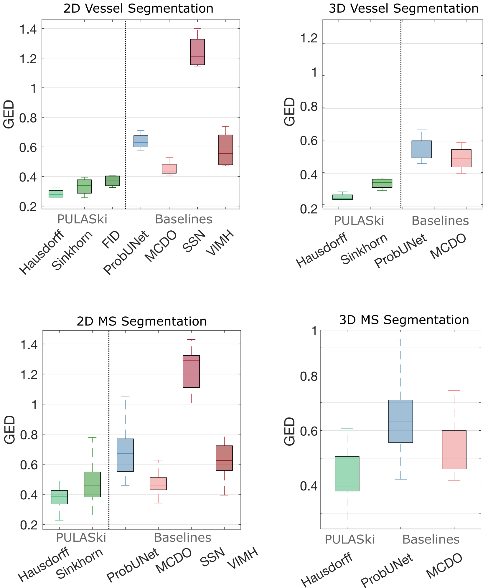
Evaluation metrics on predicted segmentations from the trained PULASKi show statistically significant improved representation of segmentation variability compared to all baselines. These conclusions hold both when training on 2D slices and 3D patches and for both the vessel and MS lesion segmentation tasks. We evaluated Generalised Energy Distances (GEDs) and Krippendorff’s alpha ($K\alpha$, see Section 4.3) across 10 generated segmentations for a given image, over 4 images in vessel segmentation and 12 MS experiments respectively, as summarised in Figure 4 and Table 1. The annotated data consists of 7 plausible annotations per image in MS and 10 in vessel. Boxplots in Figure 4 are are computed over the set of GED values calculated for each image. Table 1 shows $K\alpha$ values calculated over the entire volume ($\mathrm{K\alpha_{all}}$) and only on voxels classified as vessel or lesion in at least one annotation ($\mathrm{K\alpha_{ROI}}$). This second set of alpha values was chosen to minimise the influence of class imbalance, as only 0.13 % and 2.56 % of the overall volumes are lesions and vessels, respectively. It merits mention that the 2D PULASki FID and 3D PULASki Sinkhorn training failed to converge (i.e., got stuck in local minima), and hence were not included in the results.

PULASKi with the Hausdorff divergence shows the best performance across both experiments, in terms of both GED and $K\alpha$. It provides an improvement over the standard Probabilistic U-Net of 56 and 51 % for 2D and 3D vessel segmentation and 46 and 33 % for 2D and 3D MS lesion segmentation, in terms of the average GED. The chosen statistical distances with PULASKi more often that not provide a statistically significant improvement in terms of both evaluation metrics over baselines at the 5% significance level, particularly in the vessel segmentation task (see Table 2). PULASKi (Hausdorff) was the only method to consistently outperform baselines at the 5% significance level. Amongst the baselines methods, MCDO with FTL loss allows for the best representation of inter-rater variability in terms of both GED (average of 0.45 for 2D and 0.49 for 3D in vessel segmentation and 0.47 for 2D and 0.55 for 3D in MS segmentation) and $K\alpha$, rather surprisingly. VI-MH U-Net provides a slight improvement over the Probabilistic U-Net in the 2D experiments. The SSN was completely unable to represent the underlying variability in the training data, as evidenced by the large GED and Krippendorff alpha scores. We posit that this is due to the cross-entropy term style loss function being bad for class imbalanced data and due to the lack of regularisation, which is present in PULASKi, Probabilistic U-Net and VI-MH U-Net.

When evaluating difference in performance between 2D and 3D implementations, there is less agreement between GED trends and $K\alpha$ trends compared to overall performance between methods. For instance, the PULASKi with Hausdorff shows improvements of about 20 % in terms of $\mathrm{K\alpha_{ROI}}$ in the 2D implementation (23.63 and 31.28) compared to 3D (45.40 and 50.56) for both vessel and MS tasks, although the reverse is true with looking at median GED.

Finally, we also assessed statistical significance of differences between the ground truth and predicted distributions from the PULASKi in terms of Krippendorff alpha scores. Hausdorff 2D was the only method that did not have any statistically significant difference, as opposed to all other methods (including the baselines, p-values not shown in the table). This suggests that while our PULASKi improves on existing methods, careful choice of the statistical distance is needed to ensure an accurate representation of inter-rater variability.

Table 1: Quantitative assessment of the distribution of generated segmentations using Krippendorff’s alpha, calculated on the entire volume ($\mathrm{K\alpha_{all}}$) and only on voxels classified as vessel or lesion in at least one annotation ($\mathrm{K\alpha_{ROI}}$). Values are indicated as mean over all images $\pm$ one standard deviation.

Vessel Segmentation
	2D
	$\mathrm{K\alpha_{all}}$	$\mathrm{K\alpha_{ROI}}$
Annotation	$40.24\pm 8.62$	$22.35\pm 10.9$
PULASki HD	$50.34\pm 2.31$	$31.28\pm 2.39$
PULASki SH	$57.62\pm 1.18$	$34.96\pm 1.3$
PULASki FID	$50.21\pm 0.39$	$29.66\pm 0.61$
Prob UNet	$99.83\pm 0.01$	$63.08\pm 0.59$
MCDO UNet	$90.00\pm 1.36$	$58.71\pm 1.07$
SSN	$100.0\pm 0$	$100.0\pm 0$
VIMH	$88.78\pm 1.79$	$57.90\pm 1.22$
	3D
	$\mathrm{K\alpha_{all}}$	$\mathrm{K\alpha_{ROI}}$
Annotation	$40.24\pm 8.62$	$22.35\pm 10.9$
PULASki HD	$76.70\pm 3.05$	$50.56\pm 3.18$
PULASki SH	$82.85\pm 2.27$	$53.30\pm 2.36$
Prob UNet	$99.72\pm 0.02$	$62.74\pm 0.17$
MCDO UNet	$95.91\pm 0.55$	$62.09\pm 0.70$
MS Segmentation
	2D
	$\mathrm{K\alpha_{all}}$	$\mathrm{K\alpha_{ROI}}$
Annotation	$60.40\pm 14.06$	$27.60\pm 10.13$
PULASki HD	$62.06\pm 11.88$	$25.52\pm 9.13$
PULASki SH	$76.41\pm 10.16$	$40.75\pm 8.85$
Prob UNet	$99.93\pm 0.03$	$57.88\pm 3.70$
MCDO UNet	$82.93\pm 8.19$	$46.74\pm 6.01$
SSN	$100.0\pm 0$	$100.0\pm 0$
VIMH	$83.53\pm 14.07$	$45.78\pm 10.13$
	3D
	$\mathrm{K\alpha_{all}}$	$\mathrm{K\alpha_{ROI}}$
Annotation	$60.40\pm 14.06$	$27.60\pm 10.13$
PULASki HD	$86.58\pm 5.81$	$49.00\pm 4.31$
Prob UNet	$99.92\pm 0.03$	$58.39\pm 2.50$
MCDO UNet	$95.87\pm 2.32$	$55.47\pm 1.99$

Table 2: $p$-values obtained using the Wilcoxon rank test while comparing the different PULASki methods against the baselines and annotations combining both data sets. Significance indicated at $\alpha=0.05$ (✓: Significant, ✗: Not Significant).

	Prob UNet			MCDO UNet			SSN			VIMH			Annotation
PULASki Method	GED	$\mathrm{K\alpha_{all}}$	$\mathrm{K\alpha_{ROI}}$	GED	$\mathrm{K\alpha_{all}}$	$\mathrm{K\alpha_{ROI}}$	GED	$\mathrm{K\alpha_{all}}$	$\mathrm{K\alpha_{ROI}}$	GED	$\mathrm{K\alpha_{all}}$	$\mathrm{K\alpha_{ROI}}$	$\mathrm{K\alpha_{all}}$	$\mathrm{K\alpha_{ROI}}$
Hausdorff 2D	✓($<10^{-6}$)	✓($<10^{-4}$)	✓($<10^{-4}$)	✓($<0.001$)	✓($<10^{-4}$)	✓($<10^{-4}$)	✓($<10^{-7}$)	✓($<10^{-4}$)	✓($<10^{-4}$)	✓($<10^{-6}$)	✓($<10^{-4}$)	✓($<10^{-4}$)	✗$(0.13)$	✗$(1.0)$
Sinkhorn 2D	✓($<0.001$)	✓($<10^{-4}$)	✓($<10^{-4}$)	✗$(1.0)$	✓($<10^{-4}$)	✓($<10^{-4}$)	✓($<10^{-7}$)	✓($<10^{-4}$)	✓($<10^{-4}$)	✓($<0.01$)	✓($<10^{-4}$)	✓($<0.001$)	✓($<10^{-4}$)	✓($<10^{-4}$)
Hausdorff 3D	✓($<10^{-5}$)	✓($<10^{-4}$)	✓($<10^{-4}$)	✓($<0.01$)	✓($<10^{-4}$)	✓($<10^{-4}$)	-	-	-	-	-	-	✓($<10^{-4}$)	✓($<10^{-4}$)

5.2 Qualitative measures of predicted segmentation variability

Figure 5: Rate of occurrence (RoO) of labels across generated segmentations for a given subject. The brighter (yellow) the voxel appears, the more often it is labelled as vessel (A,C) or lesion (B,D). The annotaded data is displayed in the dashed rectangle for vessel segmentation (A) and MS lesion (B). (A) RoO for the 2D vessel segmentation for PULASki method with different loss functions (FID, Sinkhorn and Hausdorff divergence) shown in the top row; baselines (Probabilistic U-Net, MCDO, VIMH, SSN) shown in bottom row. All methods were trained on 10 plausible labels per image. A detailed view of a specific region, indicated in the red rectangle, is provied below the larger volume. (B) RoO for the 2D Multiple sclerosis segmentation for PULASki method with different loss functions (Sinkhorn and Hausdorff) and selected baselines. All methods were trained on 7 plausible labels per image. (C) and (D) RoO for the 3D implementation in vessel segmentation and MS segmentation, respectively.

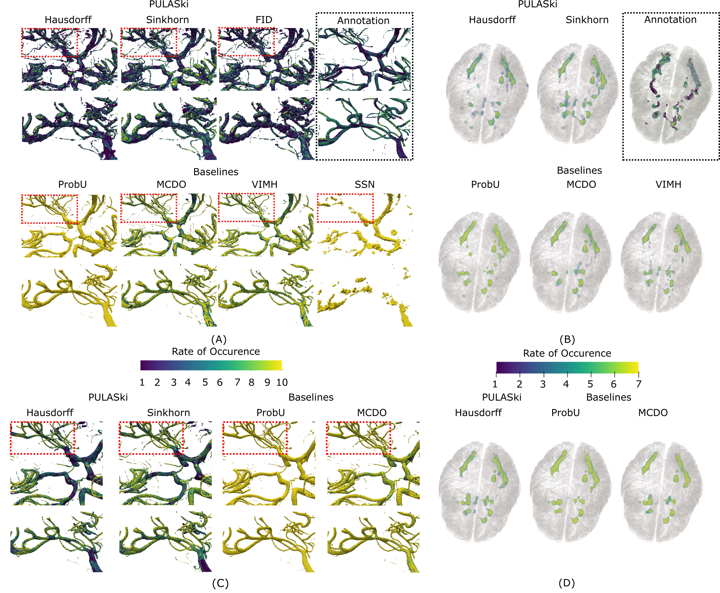
While evaluation metrics provide a concise quantitative measure of how closely the predicted distribution matches the annotations, qualitative results can be useful to determine which specific features are well represented by different methods. We plotted the frequency of labelling as vessel or lesion at a voxel level across 10 predicted segmentations from each method (Rate of Occurrence (RoO) see Figure 5. The brighter (yellow), the voxel appears, the more often it is labelled as a vessel or MS lesion throughout the output plausible segmentations. In line with the quantitative metrics, the PULASKi approach generates segmentations with structure and levels of agreement between annotations that are more consistent with the training data (see Figure 3), for both vessel and lesion segmentation. However, frequencies appear to be better represented in the vessel segmentation task than in the MS lesion task, where the extent of lesions is smaller and level of agreement across predicted segmentations higher than in the training data (see Figure 3(B)). This is true not just for PULASKi, but across all methods and could be attributed to the lower inter-rater agreement in the annotated MS data. Finally, vessel thickness and lesion extents are slightly over-estimated in the PULASKi method in 2D slice based training compared to 3D volumes.

The baseline probabilistic U-Net provides reasonable segmentations in terms of vessel structure and MS lesion shape, however it is clear from Figure 5 that the variability between segmentations is very poorly represented. Both MCDO and VI-MH U-Net demonstrate superior performance to the probabilistic U-Net; the improvement of the VI-MH over the probabilistic U-Net is much clearer in Figure 5 compared to the evaluation metrics where there was not a statistically significant difference. Consistent with the evaluation metrics, the SSN provides unrealistic, disjointed vessel segmentations and poor representation of variability. Smaller vessels are particularly poorly segmented in the SSN, suggesting that the DeepMedic architecture might not be suitable for small vessel segmentation. But the multi-scale nature of DeepMedic should have been better for large, as well as small vessels. But maybe it simply ignored the small vessels and focused only on the large vessels. The dual-pathway idea of DeepMedic might have been acting against vessels that appeared only on one pathway (higher scale). In fact, methods that are more capable of producing segmentations with less agreement between annotations are better able to segment small vessels (see red rectangle in Figure 5), although many of these vessels are unrealistically disjointed. This indicates that further refinements are needed to simultaneously segment both large and small vessels, whilst representing underlying variability in annotations.

5.3 Pixel-wise Probability Distribution

Figure 6: 3D volume of pixel-wise probability of being a vessel for 6 (exemplary chosen) of the 10 generated plausible segmentations in the 3D Hausdorff implementation. The median over the 10 output segmentations is displayed at the bottom. Higher probability of the voxel being a vessel is shown in blue, while red indicates low probability. The green arrows indicate internal vessel parts that become visible because the measurement field of view ends at that specific location.

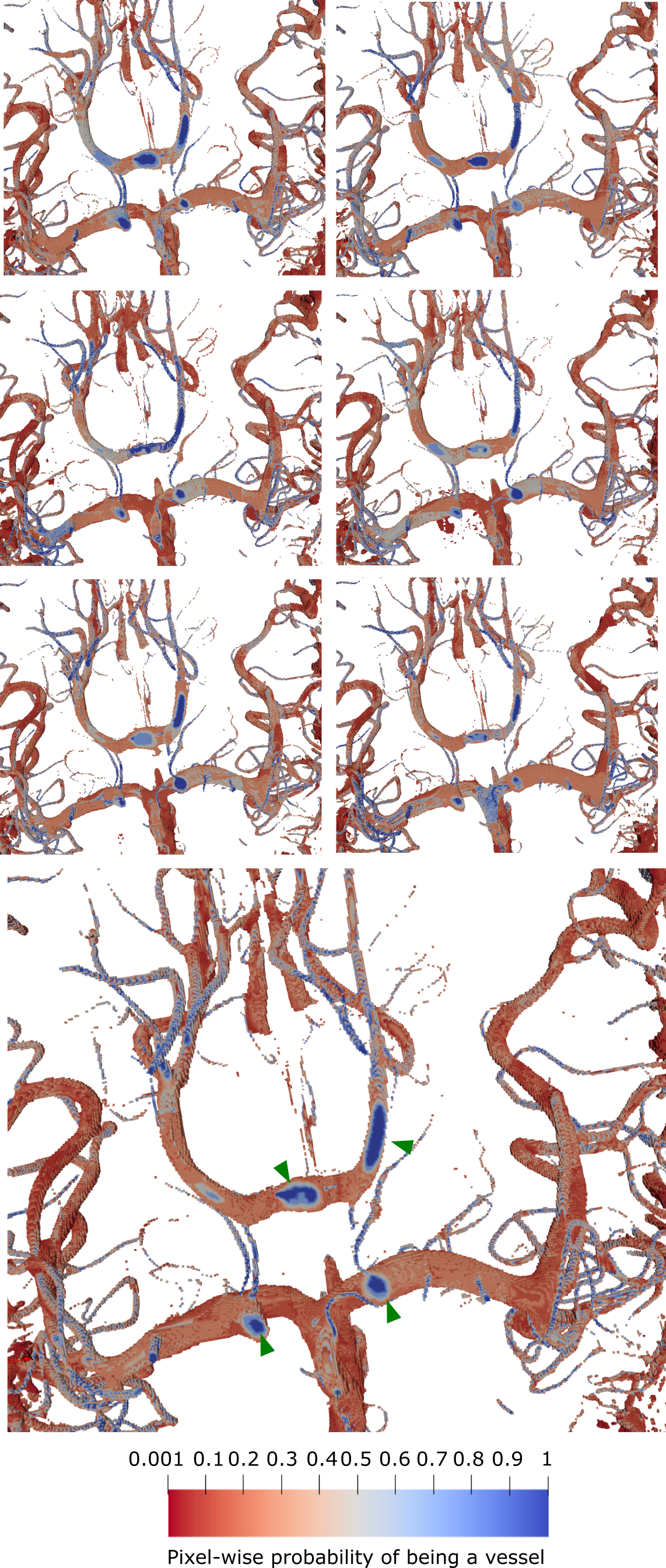
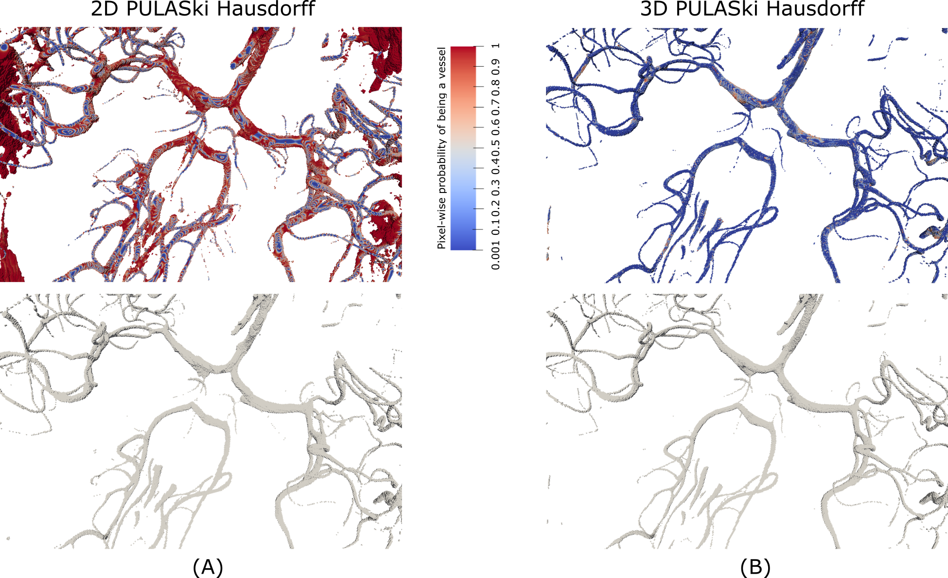
Pixel-wise class probabilities, or marginal probabilities, are useful for a variety of downstream tasks although they only partially capture the dependence structure between pixels. Such tasks include setting appropriate thresholds to estimate vessel diameter in surface mesh generation, or to estimated uncertainty of hemodynamic simulations in underlying surface meshes. Here we consider pixel-wise probabilities to be the output of the soft-max operator (i.e. the logits), noting that the probability itself is random in all methods considered. Different to the RoO discussed in Section 5.2, variations in the pixel-wise probabilities can be used as a measure of model uncertainty. As evident in Figure 6, there can often be significant variability in pixel-wise class probabilities at vessel junctions and boundaries. This holds for the PULASKi with Hausdorff divergence; similar levels of variability were not observed for the baselines method consistent with the under-estimation of uncertainty in terms of other metrics. Conversely, pixel-wise probabilities are much less variable along the vessel centreline and are closer to probability 1 than at other locations as expected.

5.4 2D vs 3D models

Figure 7: Comparison of 2D and 3D vessel segmentation for the PULASki method with Hausdorff divergence, exemplary shown for one plausible generated segmentation. The full volume is shown in the left column. Detailed views are displayed showing larger vessels (red square, middle column) and smaller vessels (blue square, right column), respectively.

Figure 8: Comparison of pixel wise probability maps (median over generated segmentations) for a given subject in 2D vs 3D Hausdorff implementation for the vessel segmentation task. The median was calculated over probability maps corresponding to 10 generated segmentations from the trained PULASKi model. The whole volume is displayed in the top row and cross sections of the middle and posterior cerebral arteries (MCA and PCA) are presented in the bottom row, with corresponding locations indicated by green lines.

Figure 9: Comparison Maximum Intensity Projection (MIP) generated from the median pixel-wise probability maps for a given subject in 2D vs 3D Hausdorff implementation for the vessel segmentation task. Results are shown for threshold of 0.5 in (A) and 0.001 in (B). The green circle encompasses a region that includes small vessels, and its sensitivity to selected thresholds is particularly pronounced in the 2D implementation.

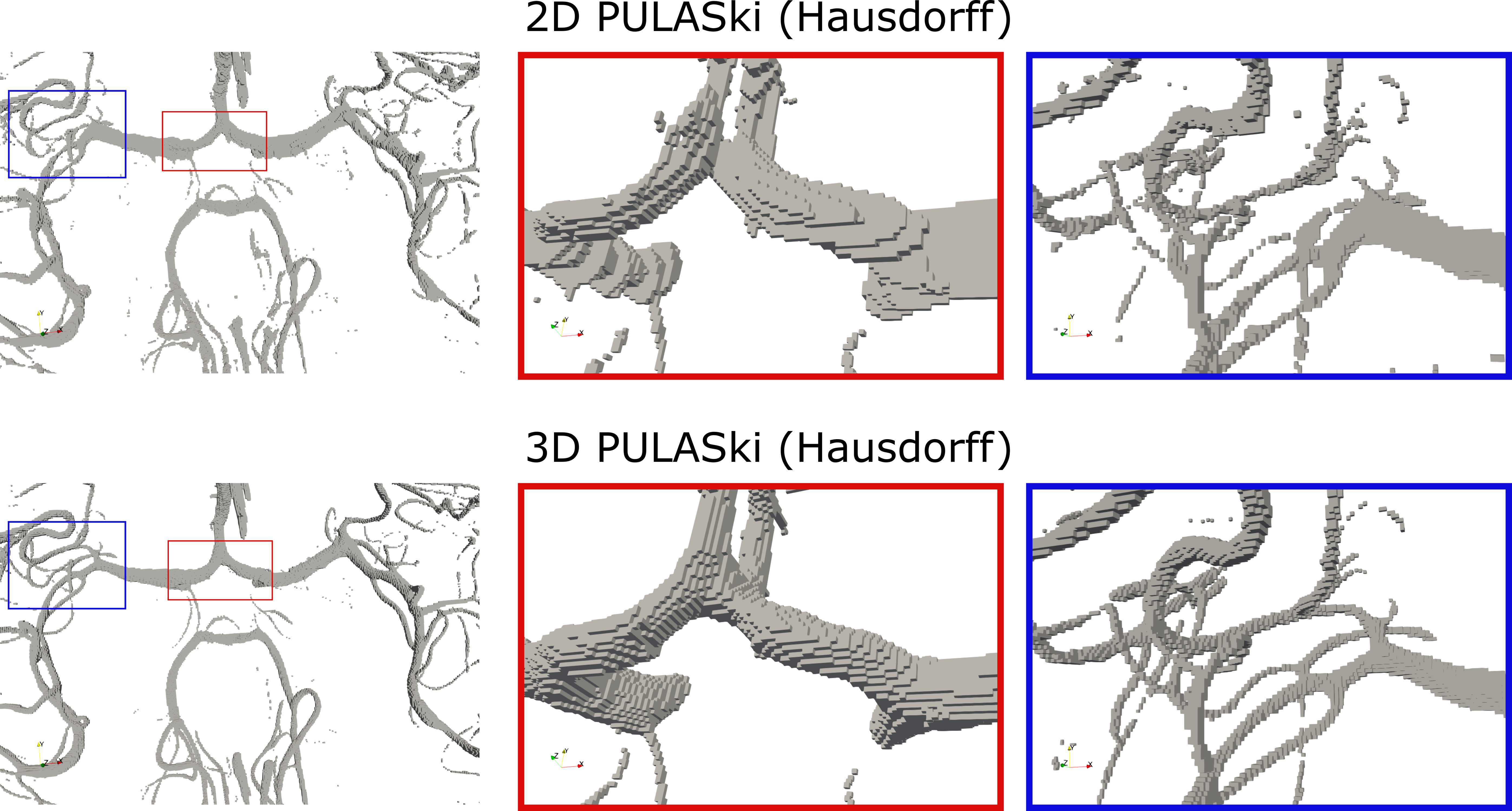
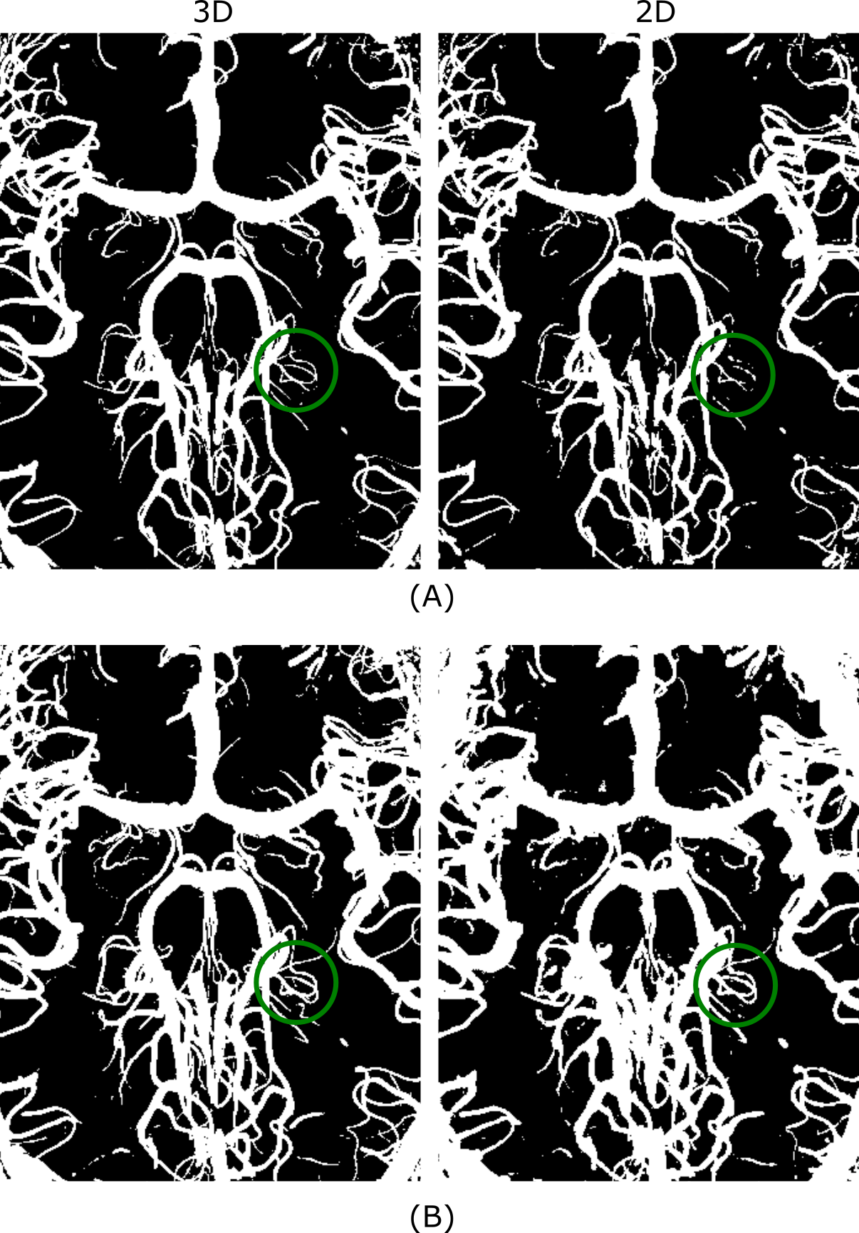
Training models to segment inherently 3D volumes using training data consisting of 2D slices, whilst computationally cheaper, generally produces poorer quality segmentations. As described in Section 5.1, GED scores were comparable between 2D and 3D implementations of the best performing method (PULASki with Hausforff distance), while the $K\alpha$ value was slightly lower for 3D compared to 2D. However, 3D mesh visualisation of the segmented vessels (Figure 7) reveals unrealistic “stacked” or “stapled” regions more prevalent in the 2D implementation than 3D. Moreover, it can be observed in Figure 8 that the pixel-wise probability of a voxel being a vessel exhibits a nearly discrete distribution of probability in 2D, whereas in 3D it gradually decreases from the centre to the edges. This can be attributed the lack of continuity between 2D slices, which is much better preserved when training on 3D patches. In the 3D implementation, predictions during inference are generated in overlapping patches. The final prediction is obtained by averaging over the overlapping region, thereby providing a better transition across patches. This makes the 3D results better suited for downstream tasks, e.g., 3D surface generation for CFD or DA, where smooth transitions are important. This smoothness can further be observed in figure 6, where pixel-wise probabilities have a much more spatially consistent structure in 3D than 2D. However, the averaging operation that allows smoother transitions in the 3D implementation has the potential to reduce variability in the generated segmentations, as indicated in Figure 5 and the higher $K\alpha$ values (Table 1). Moreover, the 3D implementation yields more certain pixel-wise probabilities. The Maximum Intensity Projection (MIP) of the pixel-wise probabilities for all values that exceed a probability of 0.5 (top row) and 0.001 (bottom row) confirm greater certainty and stability in the 3D implementation (Figure 9. Specifically, for small vessels (green circle), the 2D projection represents the area only for the lower threshold as a connected vessel segment, whereas the 3D implementation illustrates analogous structures for both thresholds. Although smaller vessels appear adequately represented in the lower threshold of the 2D segmentation, larger vessels appear to be overestimated.

Figure 10: Approximation of the most probable (maximum likelihood) segmentation from the PULASKi method in 2D (A) and 3D (B) implementation. This was calculated by adopting the prior mean for the latent vector $z$. The top row shows the corresponding pixel wise probabilities of being a vessel and the bottom row displays the final segmentation, obtained by applying Otsu’s method to threshold the probability map.

Figure 11: Surface mesh created using the most probable segmentation from the 2D (A) and 3D (B) Hausdorff PULASki implementation. The CoW region is depicted in the left column showcasing larger vessels, while the middle and right columns display zoomed views of smaller vessel structures close to the right and left middle cerebral arteries.

5.5 Anatomical plausibility of generated segmentations

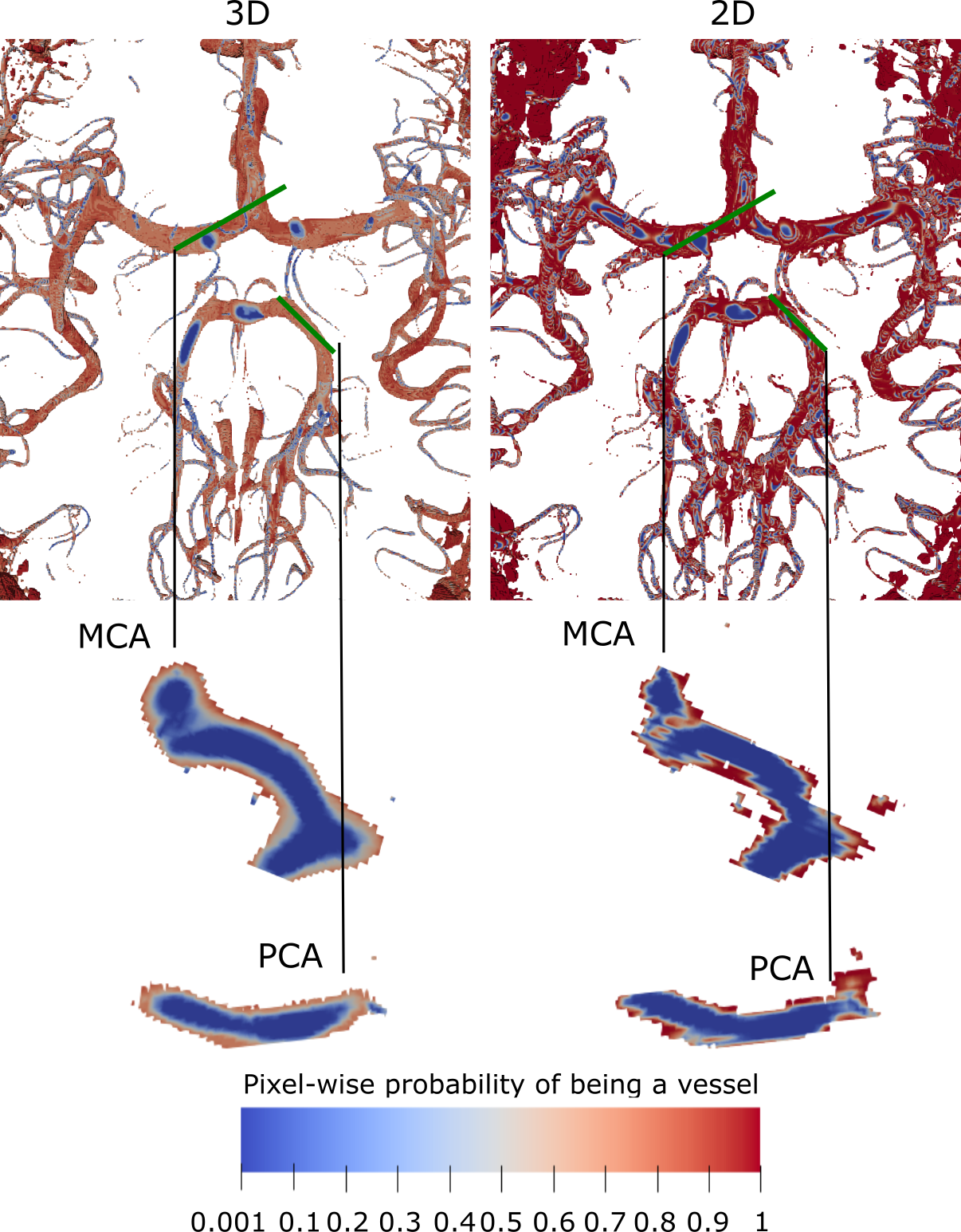
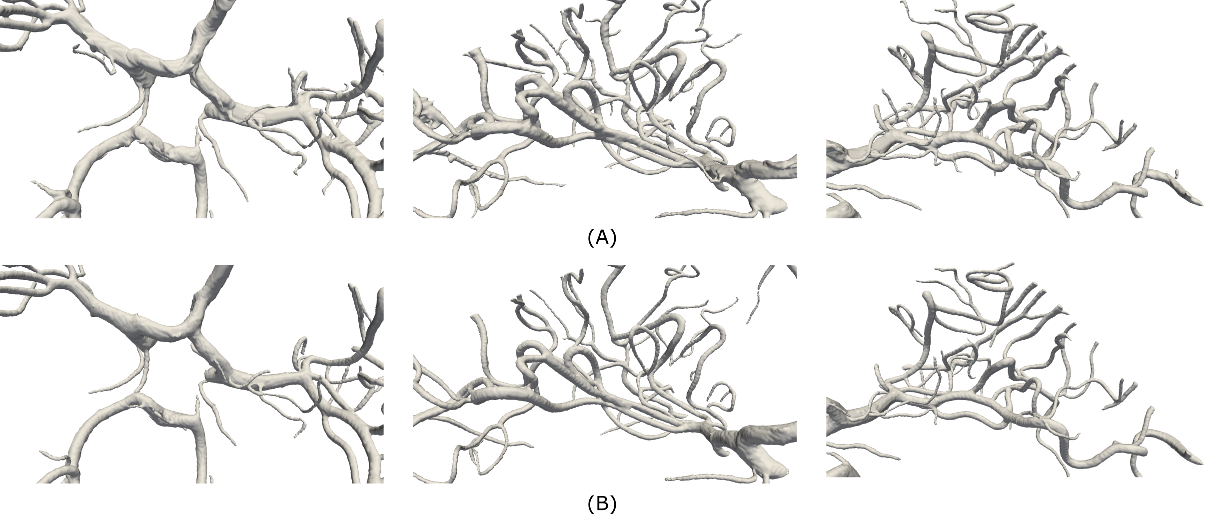
Several downstream tasks necessitate not only an estimation of the most likely segmentation, but also the generation of smooth surface meshes for the segmented volume. For instance, conducting a CFD simulation within a segmented vessel demands seamlessly connected and smooth surface structures. Figure 10 shows pixel-wise probabilities (logits) generated from the PULASKi (Hausdorff) with the prior mean of the latent variable $z$. This was then used together with Otsu’s method to generate an approximation of the most probable segmentation (Figure 11). Both 2D and 3D implementations yield segmentations that are in large part anatomically credible, in particular the Circle of Willis region is showing connected anterior, posterior and middle cerebral arteries. The left posterior communicating artery (Pcom) is reconstructed with the 3D implementaion, while the right Pcom is disconnected. However, this could also be attributed to the individual anatomy of the CoW in individual patients, which can be a physiological normal variant The most probable segmentation also appears to be significantly more anatomically credible (in terms of less stacked/stapled segmentations, disjointed vessels and smoother tube like vessel structures) than the randomly generated segmentations (see Figure 7). Most notably, Figure 10 demonstrates increased pixel-wise uncertainty in the 2D implementation relative to its 3D counterpart. This could be attributed to the fact that in 2D, the model learns and infers in a disjoint fashion (i.e., each slice is learnt and predicted independently), and also the models do not learn the relation in the $Z$ direction. While in 3D, the model learns from overlapping 3D patches, and during inference, overlapped parts of the patches are averaged – parts of the images with less certainty are averaged out, resulting in more confident segmentations. This discrepancy in 2D has implications for the generation of surface meshes necessary for CFD and other numerical simulations, as illustrated in Figure 11. As anticipated, the surface structure of the meshes is smoother in the 3D implementation (especially for the larger CoW region). Additionally, the 2D implementation has a tendency to produce thicker vessel segmentations (Figure 11) than in 3D which is in line with the higher pixel-wise uncertainty and likely due to inefficiencies of the 2D implementation rather than reflecting actual vessel thickness. However, the 2D meshes are satisfactory and could be utilised for downstream tasks with additional processing steps, such as smoothing. This may be desirable in cases where the computational overhead of a 3D implementation for training is prohibitive.

5.6 Methodological insights

Table 3: Comparison of the network architectures in terms of the number of trainable parameters

	2D	3D
Probabilistic UNets (including PULASki)	7,509,580	22,512,940
MCDO UNet	7,701,825	22,399,425
SSN	425,287	1,042,507
VIMH	1,899,968	5,519,360

Table 4: Comparison of the computational complexity of the models by the means of MACs

	MACs ($\times 10^{9}$)
	2D VSeg	2D MSSeg	3D VSeg/MSSeg
Probabilistic UNets (including PULASki)	54.75	11.51	58.61
MCDO UNet	92.70	19.48	97.63
SSN	34.93	7.34	113.70
VIMH	26.61	4.32	45.79

Table 5: Comparison of model efficiency, in terms of MACs (of the network architectures) per trainable parameter, presented in logarithmic (base 10) scale

	MACs/Parameter (log)
	2D VSeg	2D MSSeg	3D VSeg/MSSeg
Probabilistic UNets (including PULASki)	3.86	3.19	3.42
MCDO UNet	4.08	3.40	3.64
SSN	4.91	4.24	5.04
VIMH	4.15	3.36	3.92

The superior performance of PULASKi with an appropriate statistical distance compared to baselines can be primarily attributed to two factors; 1) effective learning of a low dimensional representation on which uncertainty quantification can be performed efficiently and 2) the chosen distribution based reconstruction losses that better capture inter grader variability (that is, to better learn $p(y|z,x)$). A significant challenge in the case studies considered here is class imbalance; for the MS training data only 0.13% of the full training data set corresponds to lesions and 2.56% corresponds to vessel in the intracranial vessel segmentation data on average. PULASKi is more robust to class imbalance issues than the adopted baselines, as no specific measures were adopted to deal with it while the original formulation of the Probabilistic U-Net failed to even converge during training until the cross-entropy was replaced with the Focal Tversky Loss (FTL) [13].

The chosen statistical distances in PULASKi are also numerically better suited to comparing the distribution of segmentations for a given image with the model output distribution. Empirical cross-entropy style losses used in the baselines poorly capture the variability in the conditional distribution $p(y|x)$, as the log probabilities for all segmentations, regardless of the corresponding image, are lumped together through a sum (see e.g., 12). Poor performance of the SSN can be attributed to similar issues, given the similarity of the loss function to that of the Probabilistic U-net, although there are likely additional shortcomings of the Deepmedic architecture for the tasks at hand. The lower resolution input might ignore smaller structures - a very frequent occurrence in both tasks performed here. Thed We attribute improved performance of the PULASKi using the Hausdorff divergence, over the theoretically more accurate de-biased Sinkhorn divergence to potential instabilities introduced when solving for the more complicated optimal transport loss in (32). The use of multiple “heads” in the MH VI-Unet appears to not be flexible enough to represent inter-rater variability in the examined case studies, although this could potentially be improved by increasing the number of heads. This would also then increase the computational expense.

Efficiency of the network architecture as well as accuracy of automatic segmentation methods are important, particularly when used with systems with limited hardware capabilities as often found in clinical settings. Efficiency with respect to the number of trainable parameters and computational complexity can be assessed by the Multiply-Accumulate Operations (MACs) per trainable parameter. To determine this we first calculated the MACs for a forward pass of each architecture and can be found in Table 4. Since MACs depend on input data size, there are differences between the vessel and lesion segmentation task in the 2D implementation as the input slices differ in size. However, the 3D implementation relies on patches of the same size in both tasks (see Table 4). The total number of trainable parameters was also computed for each architecture (Table 3), which also helps provide some insights as to the differing accuracy of the methods. The significantly lower number of trainable parameters in the SSN (with DeepMedic) could indicate that the architecture is not sufficiently flexible for the tasks at hand, to represent complex segmentations. The better performing methods (MCDO, PULASKi) have a similar number of trainable parameters, significantly more than in the SSN. In terms of efficiency, we see that the Probabilistic U-Net based methods (including PULASKi) are most efficient (Table 5), with SSN the least efficient despite the very low number of trainable parameters. However, it is worth mentioning that during training, there are additional overheads (e.g., loss calculation and backward pass), and the best performing distances (Hausdorff and Sinkhorn) are computationally more expensive than evaluating the cross-entropy.

6 Discussion

Segmenting complex vessel geometries and tissue lesions from noisy MRI remains a challenging task, despite improvements in imaging technology. Often times there is significant variation in labels from human annotators for the same image. Supervised and semi-supervised deep learning based segmentation is rapidly developing to provide more accurate results in a fraction of the time of traditional methods. Ensuring these methods faithfully capture the underlying uncertainty in labelled data is paramount, so as to prevent over-confident diagnoses of diseases and model predictions. Our method provides a significant improvement on many existing methods for capturing inter-rater variability in deep learning based medical image segmentation, for the same amount of training data. It is easily implementable and can be used to provide practitioners with pixel-wise uncertainties and generate several whole volume plausible segmentations for ensemble-based modelling purposes involving computational fluid dynamics models and data assimilation [8].

Experimental results on intracranial image segmentation tasks show that the distribution based loss functions utilised in our proposed method, PULASKi, drastically improve the ability to learn diverse plausible segmentations for a given image. The loss functions are also far less sensitive to class imbalance in the training data set, based on experiments in both vessel and multiple sclerosis segmentation tasks in 2D and 3D cases. Furthermore, there are minimal extra hyper-parameters to be specified compared to existing methods (e.g., probabilistic U-net), whilst simultaneously providing dramatic improvement in performance. Our experimental results also demonstrate a significant improvement in both the anatomical plausibility of generated segmentations and representation of uncertainty when training on 3D patches rather than 2D slices. In particular, vessel thickness seems to be overestimated easily in the 2D implementation with an uncertain threshold and vessel boundaries are not as smooth as in 3D.

The representation of small vessels is drastically improved using 3D training data, a task that has traditionally been incredibly challenging. Manual and semi-automated segmentation, despite being time-consuming, is typically deemed reliable primarily for medium to large vessels, as indicated in previous studies [57, 12]. The proposed work is one of the first studies to demonstrate reliable segmentation of small vessels and supports the results of [12] by producing a set of plausible segmentations. Moreover, PULASki was the only method showing variability in the subset of possible segmentations within the area of smaller vessels, as illustrated in the RoO results (Figure 5) This also aligns more closely with the annotated data, as depicted in 3. This provides significant opportunity to improve the modeling of cerebral small-vessel which supports the research in diseases that are difficult to predict and manage, e.g., CSVD. In the MS segmentation task, PULASKi also provides an improved representation of inter-rater variability over the baselines, although “outlier” or “extreme” annotations are still not represented well. This suggests potential for further improvements to quantify distributional tails more accurately. 5

While PULASki, as well as the baseline methods presented here, are aimed at providing multiple plausible segmentations. However, there can be situations where obtaining one single segmentation per input is required (e.g. at clinics). In such scenarios, majority voting from the predicted plausible segmentations can be taken, or even the segmentation from the prior mean can be utilised.

It should be noted that the distribution-based loss functions in PULASKi are more computationally expensive to evaluate than the standard cross-entropy or FTL used in the benchmark methods. However, we anticipate that this is generally not prohibitive, as training is typically undertaken offline and there is no further computational burden for inference tasks, compared to other variational autoencoder based methods.

References

- [1] Y. Li, J. Ni, A. Elazab, J. Wu, Multiple self-attention network for intracranial vessel segmentation, in: 2021 International Joint Conference on Neural Networks (IJCNN), IEEE, 2021, pp. 1–8.
- [2] J. Ni, J. Wu, H. Wang, J. Tong, Z. Chen, K. K. Wong, D. Abbott, Global channel attention networks for intracranial vessel segmentation, Computers in biology and medicine 118 (2020) 103639.
- [3] S. Chatterjee, A. Sciarra, M. Dünnwald, P. Tummala, S. K. Agrawal, A. Jauhari, A. Kalra, S. Oeltze-Jafra, O. Speck, A. Nürnberger, Strega: Unsupervised anomaly detection in brain mris using a compact context-encoding variational autoencoder, Computers in Biology and Medicine 149 (2022) 106093.
- [4] M. Antonelli, A. Reinke, S. Bakas, K. Farahani, A. Kopp-Schneider, B. A. Landman, G. Litjens, B. Menze, O. Ronneberger, R. M. Summers, et al., The medical segmentation decathlon, Nature communications 13 (1) (2022) 4128.
- [5] I. Qureshi, J. Yan, Q. Abbas, K. Shaheed, A. B. Riaz, A. Wahid, M. W. J. Khan, P. Szczuko, Medical image segmentation using deep semantic-based methods: A review of techniques, applications and emerging trends, Information Fusion 90 (2023) 316–352.
- [6] S. Czolbe, K. Arnavaz, O. Krause, A. Feragen, Is segmentation uncertainty useful?, in: International Conference on Information Processing in Medical Imaging, Springer, 2021, pp. 715–726.
- [7] G. Varoquaux, V. Cheplygina, Machine learning for medical imaging: methodological failures and recommendations for the future, NPJ digital medicine 5 (1) (2022) 48.
- [8] F. Gaidzik, S. Pathiraja, S. Saalfeld, D. Stucht, O. Speck, D. Thévenin, G. Janiga, Hemodynamic data assimilation in a subject-specific circle of willis geometry, Clinical Neuroradiology 31 (3) (2021) 643–651.
- [9] C. Chen, C. Qin, H. Qiu, G. Tarroni, J. Duan, W. Bai, D. Rueckert, Deep learning for cardiac image segmentation: a review, Frontiers in Cardiovascular Medicine 7 (2020) 25.
- [10] O. Ronneberger, P. Fischer, T. Brox, U-net: Convolutional networks for biomedical image segmentation, in: Medical Image Computing and Computer-Assisted Intervention–MICCAI 2015: 18th International Conference, Munich, Germany, October 5-9, 2015, Proceedings, Part III 18, Springer, 2015, pp. 234–241.
- [11] O. Oktay, J. Schlemper, L. L. Folgoc, M. Lee, M. Heinrich, K. Misawa, K. Mori, S. McDonagh, N. Y. Hammerla, B. Kainz, et al., Attention u-net: Learning where to look for the pancreas, arXiv preprint arXiv:1804.03999.
- [12] S. Chatterjee, K. Prabhu, M. Pattadkal, G. Bortsova, C. Sarasaen, F. Dubost, H. Mattern, M. de Bruijne, O. Speck, A. Nürnberger, Ds6, deformation-aware semi-supervised learning: Application to small vessel segmentation with noisy training data, Journal of Imaging 8 (10) (2022) 259.
- [13] N. Abraham, N. M. Khan, A novel focal tversky loss function with improved attention u-net for lesion segmentation, in: 2019 IEEE 16th international symposium on biomedical imaging (ISBI 2019), IEEE, 2019, pp. 683–687.
-
[14]
M. Monteiro, L. Le Folgoc, D. Coelho de Castro, N. Pawlowski, B. Marques,
K. Kamnitsas, M. van der Wilk, B. Glocker,
Stochastic
segmentation networks: Modelling spatially correlated aleatoric uncertainty,
in: H. Larochelle, M. Ranzato, R. Hadsell, M. Balcan, H. Lin (Eds.), Advances
in Neural Information Processing Systems, Vol. 33, Curran Associates, Inc.,
2020, pp. 12756–12767.
URL https://proceedings.neurips.cc/paper/2020/file/95f8d9901ca8878e291552f001f67692-Paper.pdf - [15] M. C. Krygier, T. LaBonte, C. Martinez, C. Norris, K. Sharma, L. N. Collins, P. P. Mukherjee, S. A. Roberts, Quantifying the unknown impact of segmentation uncertainty on image-based simulations, Nature communications 12 (1) (2021) 5414.
- [16] J. Caldeira, B. Nord, Deeply uncertain: comparing methods of uncertainty quantification in deep learning algorithms, Machine Learning: Science and Technology 2 (1) (2020) 015002.
- [17] Y. Li, S. Rao, A. Hassaine, R. Ramakrishnan, D. Canoy, G. Salimi-Khorshidi, M. Mamouei, T. Lukasiewicz, K. Rahimi, Deep bayesian gaussian processes for uncertainty estimation in electronic health records, Scientific reports 11 (1) (2021) 20685.
- [18] M. Abdar, F. Pourpanah, S. Hussain, D. Rezazadegan, L. Liu, M. Ghavamzadeh, P. Fieguth, X. Cao, A. Khosravi, U. R. Acharya, et al., A review of uncertainty quantification in deep learning: Techniques, applications and challenges, Information fusion 76 (2021) 243–297.
- [19] Y. Kwon, J.-H. Won, B. J. Kim, M. C. Paik, Uncertainty quantification using bayesian neural networks in classification: Application to biomedical image segmentation, Computational Statistics & Data Analysis 142 (2020) 106816.
- [20] I. Khemakhem, D. Kingma, R. Monti, A. Hyvarinen, Variational autoencoders and nonlinear ica: A unifying framework, in: International Conference on Artificial Intelligence and Statistics, PMLR, 2020, pp. 2207–2217.
- [21] Y. Gal, Z. Ghahramani, Dropout as a bayesian approximation: Representing model uncertainty in deep learning, in: international conference on machine learning, PMLR, 2016, pp. 1050–1059.
[22]
A. Mobiny, P. Yuan, S. K. Moulik, N. Garg, C. C. Wu, H. Van Nguyen,
DropConnect is effective
in modeling uncertainty of Bayesian deep networks, Scientific Reports
11 (1) (2021) 1–14.
arXiv:1906.04569,
doi:10.1038/s41598-021-84854-x.
URL https://doi.org/10.1038/s41598-021-84854-x - [23] G. E. Hinton, N. Srivastava, A. Krizhevsky, I. Sutskever, R. R. Salakhutdinov, Improving neural networks by preventing co-adaptation of feature detectors, arXiv preprint arXiv:1207.0580.
- [24] J. Tompson, R. Goroshin, A. Jain, Y. LeCun, C. Bregler, Efficient object localization using convolutional networks, in: Proceedings of the IEEE conference on computer vision and pattern recognition, 2015, pp. 648–656.
- [25] S. Kohl, B. Romera-Paredes, C. Meyer, J. De Fauw, J. R. Ledsam, K. Maier-Hein, S. A. Eslami, D. J. Rezende, O. Ronneberger, A probabilistic u-net for segmentation of ambiguous images, in: Advances in neural information processing systems, 2018, pp. 6965–6975.
- [26] M. Fuchs, C. Gonzalez, A. Mukhopadhyay, Practical uncertainty quantification for brain tumor segmentation, in: International Conference on Medical Imaging with Deep Learning, PMLR, 2022, pp. 407–422.
- [27] M. R. Rezaei-Dastjerdehei, A. Mijani, E. Fatemizadeh, Addressing imbalance in multi-label classification using weighted cross entropy loss function, in: 2020 27th National and 5th International Iranian Conference on Biomedical Engineering (ICBME), IEEE, 2020, pp. 333–338.
- [28] J. Tian, N. C. Mithun, Z. Seymour, H.-P. Chiu, Z. Kira, Striking the right balance: Recall loss for semantic segmentation, in: 2022 International Conference on Robotics and Automation (ICRA), IEEE, 2022, pp. 5063–5069.
- [29] F. Fan, J. L. Saver, Neurovascular disease is the second leading cause of death in the united states (us): A modern disease burden analysis, Stroke 49 (Suppl_1) (2018) A169–A169.
- [30] B. C. Campbell, D. A. De Silva, M. R. Macleod, S. B. Coutts, L. H. Schwamm, S. M. Davis, G. A. Donnan, Ischaemic stroke, Nature reviews Disease primers 5 (1) (2019) 70.
- [31] S. Singh, N. Mittal, H. Singh, D. Oliva, Improving the segmentation of digital images by using a modified otsu’s between-class variance, Multimedia Tools and Applications (2023) 1–43.
- [32] N. Otsu, A threshold selection method from gray-level histograms, IEEE transactions on systems, man, and cybernetics 9 (1) (1979) 62–66.
- [33] I. Higgins, L. Matthey, A. Pal, C. Burgess, X. Glorot, M. Botvinick, S. Mohamed, A. Lerchner, beta-VAE: Learning basic visual concepts with a constrained variational framework, in: ICLR, 2017. doi:10.1177/1078087408328050.
- [34] D. P. Kingma, M. Welling, An introduction to variational autoencoders, Foundations and Trends in Machine Learning 12 (4) (2019) 307–392. arXiv:1906.02691, doi:10.1561/2200000056.
- [35] T. Poggio, Q. Liao, A. Banburski, Complexity control by gradient descent in deep networks, Nature communications 11 (1) (2020) 1027.
- [36] A. Kendall, V. Badrinarayanan, R. Cipolla, Bayesian segnet: Model uncertainty in deep convolutional encoder-decoder architectures for scene understanding, arXiv preprint arXiv:1511.02680.
- [37] Y. Gal, Z. Ghahramani, Dropout as a bayesian approximation: Representing model uncertainty in deep learning, in: international conference on machine learning, PMLR, 2016, pp. 1050–1059.
[38]
I. Tolstikhin, O. Bousquet, S. Gelly, B. Schoelkopf,
Wasserstein
Auto-encoders, in: ICLR, 2018, pp. 1–16.
URL http://www.niassembly.gov.uk/globalassets/documents/raise/publications/2015/general/9915.pdf - [39] M. Heusel, H. Ramsauer, T. Unterthiner, B. Nessler, S. Hochreiter, GANs trained by a two time-scale update rule converge to a local Nash equilibrium, Advances in Neural Information Processing Systems 2017-December (Nips) (2017) 6627–6638. arXiv:1706.08500.
- [40] M. Bińkowski, D. J. Sutherland, M. Arbel, A. Gretton, Demystifying mmd gans, in: International Conference on Learning Representations, 2018.
- [41] C. Szegedy, V. Vanhoucke, S. Ioffe, J. Shlens, Z. Wojna, Rethinking the inception architecture for computer vision, in: Proceedings of the IEEE conference on computer vision and pattern recognition, 2016, pp. 2818–2826.
- [42] J. Feydy, Geometric data analysis, beyond convolutions, Ph.D. thesis (2020). doi:10.4324/9781315516257-1.
- [43] A. Ramdas, N. G. Trillos, M. Cuturi, On wasserstein two-sample testing and related families of nonparametric tests, Entropy 19 (2) (2017) 1–15. arXiv:1509.02237, doi:10.3390/e19020047.
[44]
A. Genevay, G. Peyre, M. Cuturi,
Learning generative
models with sinkhorn divergences, in: A. Storkey, F. Perez-Cruz (Eds.),
Proceedings of the Twenty-First International Conference on Artificial
Intelligence and Statistics, Vol. 84 of Proceedings of Machine Learning
Research, PMLR, 2018, pp. 1608–1617.
URL https://proceedings.mlr.press/v84/genevay18a.html - [45] C. O. Häusler, M. Hanke, A studyforrest extension, an annotation of spoken language in the german dubbed movie “forrest gump” and its audio-description, F1000Research 10.
- [46] A. F. Frangi, W. J. Niessen, K. L. Vincken, M. A. Viergever, Multiscale vessel enhancement filtering, in: International conference on medical image computing and computer-assisted intervention, Springer, 1998, pp. 130–137.
- [47] O. Commowick, M. Kain, R. Casey, R. Ameli, J.-C. Ferré, A. Kerbrat, T. Tourdias, F. Cervenansky, S. Camarasu-Pop, T. Glatard, et al., Multiple sclerosis lesions segmentation from multiple experts: The miccai 2016 challenge dataset, Neuroimage 244 (2021) 118589.
- [48] A. Paszke, S. Gross, F. Massa, A. Lerer, J. Bradbury, G. Chanan, T. Killeen, Z. Lin, N. Gimelshein, L. Antiga, et al., Pytorch: An imperative style, high-performance deep learning library, Advances in neural information processing systems 32.
- [49] F. Pérez-García, R. Sparks, S. Ourselin, Torchio: a python library for efficient loading, preprocessing, augmentation and patch-based sampling of medical images in deep learning, Computer Methods and Programs in Biomedicine 208 (2021) 106236.
- [50] J. Feydy, T. Séjourné, F.-X. Vialard, S.-i. Amari, A. Trouve, G. Peyré, Interpolating between optimal transport and mmd using sinkhorn divergences, in: The 22nd International Conference on Artificial Intelligence and Statistics, 2019, pp. 2681–2690.
- [51] J. Petersen, P. F. Jäger, F. Isensee, S. A. Kohl, U. Neuberger, W. Wick, J. Debus, S. Heiland, M. Bendszus, P. Kickingereder, et al., Deep probabilistic modeling of glioma growth, in: Medical Image Computing and Computer Assisted Intervention–MICCAI 2019: 22nd International Conference, Shenzhen, China, October 13–17, 2019, Proceedings, Part II 22, Springer, 2019, pp. 806–814.
- [52] S. Rajaraman, G. Zamzmi, S. K. Antani, Novel loss functions for ensemble-based medical image classification, Plos one 16 (12) (2021) e0261307.
[53]
K. Kamnitsas, C. Ledig, V. F. J. Newcombe, J. P. Simpson, A. D. Kane, D. K.
Menon, D. Rueckert, B. Glocker,
Efficient
multi-scale 3D CNN with fully connected CRF for accurate brain lesion
segmentation, Medical Image Analysis 36 (2017) 61–78.
doi:https://doi.org/10.1016/j.media.2016.10.004.
URL https://www.sciencedirect.com/science/article/pii/S1361841516301839 - [54] G. J. Székely, M. L. Rizzo, Energy statistics: A class of statistics based on distances, Journal of statistical planning and inference 143 (8) (2013) 1249–1272.
- [55] K. Krippendorff, Content analysis: An introduction to its methodology, Sage publications, 2018.
- [56] F. Wilcoxon, Individual comparisons by ranking methods, in: Breakthroughs in Statistics: Methodology and Distribution, Springer, 1992, pp. 196–202.
- [57] T. Jerman, F. Pernuš, B. Likar, Ž. Špiclin, Beyond frangi: an improved multiscale vesselness filter, in: Medical Imaging 2015: Image Processing, Vol. 9413, SPIE, 2015, pp. 623–633.