AdamL: A fast adaptive gradient method
incorporating loss function

Abstract

Adaptive first-order optimizers are fundamental tools in deep learning, although they may suffer from poor generalization due to the nonuniform gradient scaling. In this work, we propose AdamL, a novel variant of the Adam optimizer, that takes into account the loss function information to attain better generalization results. We provide sufficient conditions that together with the Polyak-Łojasiewicz inequality, ensure the linear convergence of AdamL. As a byproduct of our analysis, we prove similar convergence properties for the EAdam, and AdaBelief optimizers. Experimental results on benchmark functions show that AdamL typically achieves either the fastest convergence or the lowest objective function values when compared to Adam, EAdam, and AdaBelief. These superior performances are confirmed when considering deep learning tasks such as training convolutional neural networks, training generative adversarial networks using vanilla convolutional neural networks, and long short-term memory networks. Finally, in the case of vanilla convolutional neural networks, AdamL stands out from the other Adam’s variants and does not require the manual adjustment of the learning rate during the later stage of the training.

Keywords: adaptive gradient methods, non-convex optimization, convergence analysis

1 Introduction

First-order optimization approaches, e.g., stochastic gradient descent (with momentum) methods (SGD) (Robbins and Monro, 1951), prevail in the training of deep neural networks due to their simplicity. However, the constant learning stepsize along each gradient coordinate generally limits the convergence speed of SGD. This can be addressed by adaptive gradient methods, such as Adagrad (Duchi et al., 2011), RMSProp (Tieleman and Hinton, 2012) and Adam (Kingma and Ba, 2014). Adam, which is arguably the most used optimizer, combines the main ingredients from the SGD with momentum (Qian, 1999) and RMSprop.

Although at early stages of training the adaptive methods usually show a faster decay of the objective function value than SGD, their convergence becomes slower at later stages (Keskar and Socher, 2017; Wilson et al., 2017). Furthermore, the nonuniform scaling of the gradient may cause worse performances on the unseen data, a phenomenon that is often called poor generalization (Hoffer et al., 2017; Keskar and Socher, 2017).

Prior Work. Many techniques have been merged to bridge the generation gap between adaptive and non-adaptive gradient methods. For instance, the procedure SWATS, proposed in (Keskar and Socher, 2017), switches from Adam to SGD when a triggering condition is satisfied. Another example is the method Adabound (Luo et al., 2019) that applies a smooth transition from adaptive methods to SGD as the time step increases, by means of dynamic bounds on the learning rates.

A recent study introduces a variant of the Adam optimizer called AdaBelief (Zhuang et al., 2020), which achieves the initial fast convergence of adaptive methods, good generalization as SGD, and training stability in complex settings such as generative adversarial networks (GANs). Adabelief is obtained from Adam by replacing the exponential moving average of the squares of the gradients, used to estimate the second moment, with the difference between the true gradient and its first moment; the authors call this quantity the “belief” term. Finally, AdaBelief adds a small positive constant $\varepsilon$ at each iteration to its second moment estimate. It is claimed that by using the “belief” term, AdaBelief considers the curvature of the objective function to improve the convergence (Zhuang et al., 2020, Sec. 2.2). However, it has been empirically demonstrated on test cases from image classification, language modeling, and object detection, that modifying the Adam scheme by simply adding the constant $\varepsilon$ to its second moment estimate, yields comparable performances as AdaBelief (Yuan and Gao, 2020). The method obtained with such a modification is called EAdam. The similar performances of EAdam and AdaBelief in these case studies require further investigations and are the main motivation of this work.

These variants of the Adam optimizer such as Adabound, AdaBelief, and EAdam are empirically shown to achieve faster convergence and better generalization performances than Adam. The convergence is normally proven by measuring the algorithm regret $R_{k}$, after a certain number of iteration steps $k$, and by showing that either $\lim_{k\to\infty}\tfrac{R_{k}}{k}=0$ or that $\lim_{k\to\infty}\nabla f(\mathbf{x}^{(k)})=\mathbf{0}$ (Kingma and Ba, 2014; Luo et al., 2019; Zhuang et al., 2020). However, the convergence analyses developed so far do not provide tools for comparing the convergence rates of the different optimizers. From a theoretical perspective, it remains uncertain whether there is an optimizer that is superior to the others, even in specific scenarios. In general, there is a lack of comparisons of the convergence rates of adaptive gradient optimizers.

Contribution of the paper. Inspired by the body of work on Adam-type optimizers, we propose a novel adaptive optimization method that we call AdamL. This method incorporates information from the loss function by linking the magnitude of the update to the distance between the value of the objective function at the current iterate and the optimum. When the loss function is not directly accessible, i.e. the optimal value is unknown, a dynamic approximation strategy can be employed. The idea is to improve the adaptivity of the scheme by taking small steps when the loss function is small and large steps otherwise. AdamL has also the advantage that it does not need a user that manually decreases the learning rate at the late stage of the training, e.g., when training convolutional neural networks.

On the theoretical side, we study and compare the convergence properties of the EAdam, AdaBelief, and AdamL optimizers, under the Polyak-Łojasiewicz (PL) inequality. Within this context, we provide sufficient conditions for the monotonicity and linear convergence of the above Adam’s variants. Moreover, we discuss the relation between these conditions and two phases that are often encountered in the execution of Adam’s variants. In the first phase, the methods behave similarly to SGD with decreasing learning rate with respect to the iteration steps; in the second phase, they perform like Adam. Finally, we perform extensive numerical tests to show that with a proper scaling strategy of the loss function, the AdamL optimizer yields faster and more stable convergence than the other adaptive gradient optimizers (Adam, AdaBelief, and EAdam). The considered case studies involve image classification tasks on the Cifar10 and Cifar100 datasets, language modeling on Penn Treebank, and the training of WGANs on Cifar10 and Anime Faces.

Outline. A review of the considered adaptive gradient methods is presented in section 2. The AdamL method is introduced in subsection 2.3. In section 3, we introduce a framework for analyzing the monotonicity and convergence rate of adaptive gradient methods under the assumption of an objective function satisfying the PL inequality. The main theoretical results are given in Propositions 1–6. The performance of AdamL is validated and compared with those of the other optimizers in section 4. Conclusions are drawn in section 5.

Notation. Throughout the paper we use bold lower case letters, e.g. $\mathbf{g}$, for vectors; superscripted case letters, e.g., $\mathbf{g}^{(k)}$ for the $k$th iteration step dependency; subscripted case letters, e.g., $g_{i}$ for the $i$th element of the vector; lower case Greek letters, for scalars. For the ease of readability, all the operations on/between vectors are elementary-wise, e.g., $\tfrac{{\bf m}^{(k)}}{\mathbf{g}^{(k)}}$, $({\mathbf{g}}^{(k)})^{2}$, $\sqrt{\mathbf{g}^{(k)}}$ and $|\,\mathbf{g}^{(k)}\,|$ represent the component-wise division, square, square root and absolute value on $\mathbf{g}^{(k)}$, respectively. When we write an operation between a vector and a scalar, we mean the component-wise operation between the former and a vector having all entries equal to the scalar. For instance, $\frac{\delta}{\mathbf{g}+\varepsilon}$ indicates the vector with entries $\frac{\delta}{g_{i}+\varepsilon}$.

2 Adaptive gradient optimization methods

This work is concerned with the following stochastic optimization problem

$$\min_{\mathbf{x}\in\mathcal{X}}\{f(\mathbf{x}):=\mathrm{E}_{\xi\sim\mathcal{D}}\,[\,F(\bf x,\xi)\,]\},$$ (1)

where $\mathcal{X}\subset\mathbb{R}^{n}$ is a nonempty compact set, $\xi$ is a random vector whose probability distribution $P$ is supported on set $\mathcal{D}\subset\mathbb{R}^{r}$ and $F:\mathcal{X}\times\mathcal{D}\to\mathbb{R}$. Concerning the objective function, we make the following assumptions that are common to many other studies on the convergence analysis of stochastic optimization, e.g. see (Kingma and Ba, 2014; Luo et al., 2019; Nemirovski et al., 2009; Ghadimi et al., 2016; Ghadimi and Lan, 2013; Nguyen et al., 2019).

Assumption 1

The function $f:\mathbb{R}^{n}\to\mathbb{R}$ satisfies the PL inequality, $F(\cdot,\xi)$ is $L$-smooth for every realization of $\xi$, the stochastic gradient $\nabla_{\mathbf{x}}F(\mathbf{x},\xi)$ is bounded and unbiased for every $\xi\in\mathcal{D}$, and the variance of $\nabla_{\mathbf{x}}F(\mathbf{x},\xi)$ is uniformly bounded. In particular, there exist constants $\sigma,\mu,L,G>0$ such that the following inequalities hold:

$$2\mu\,(f(\mathbf{x})-f^{*}) \leq\|\nabla f(\mathbf{x})\|^{2},$$ (2)

$$\|\nabla_{\mathbf{x}}F(\mathbf{x}_{1},\xi)-\nabla_{\mathbf{x}}F(\mathbf{x}_{2},\xi)\| \leq L\,\|\mathbf{x}_{1}-\mathbf{x}_{2}\|,$$ (3)

$$\mathrm{E}\,[\,\nabla_{\mathbf{x}}F(\mathbf{x},\xi)\,] =\nabla f(\mathbf{x}),$$ (4)

$$\|\nabla_{\mathbf{x}}F(\mathbf{x},\xi)\|_{\infty} \leq G,$$ (5)

$$0\leq\mathrm{E}\,[\,\|\nabla_{\mathbf{x}}F(\mathbf{x},\xi)\|^{2}\,] -\|\nabla f(\mathbf{x})\|^{2}\leq\sigma^{2},$$ (6)

for any $\mathbf{x},\mathbf{x}_{1},\mathbf{x}_{2}\in\mathbb{R}^{n}$.

Note that Eq. 4 always holds if $f(\cdot)$ is finite valued in a neighborhood of a point $x$ (Nemirovski et al., 2009, cf. (13)). On the basis of Eq. 3, Eq. 4, and Jensen’s inequality, we have that

$$\|\nabla f(\mathbf{x}_{1})-\nabla f(\mathbf{x}_{2})\| \leq L\,\|\mathbf{x}_{1}-\mathbf{x}_{2}\|.$$ (7)

2.1 Algorithms

Let us review the Adam method and two of its variants, namely EAdam and Adabelief. Adam combines the main schemes of two other popular optimizers, i.e., momentum and RMSProp. Similar to momentum, the Adam optimizer updates the parameters using the exponential moving average (EMA) of the gradient $\nabla_{\mathbf{x}}F(\mathbf{x}^{(k)},\xi)$, i.e., the first raw moment estimate. The learning rate is scaled with the same rule of RMSProp, i.e., the EMA of the squared gradient, namely the second raw moment estimate. Since the first and second raw moment estimates are biased by their initialization, a bias correction is applied. EAdam and AdaBelief follow the same updating scheme as Adam, with the exception that they employ alternative second moment estimates, as outlined in Table 1. In Algorithm 1, we present a general template of these adaptive gradient methods; to obtain a specific optimizer it is sufficient to define $\boldsymbol{\eta}^{(k)}$ in the while loop with the corresponding second raw moment estimate in Table 1: $\mathbf{v}^{(k)}$ for Adam, $\mathbf{y}^{(k)}$ for EAdam, and $\mathbf{s}^{(k)}$ for AdaBelief. The hyperparameters $\beta_{1},\beta_{2}\in(0,1)$ control the exponential decay rates of these moving averages and $\eta>0$ affects the magnitude of the learning rate. For a detailed description of these algorithms see (Kingma and Ba, 2014; Yuan and Gao, 2020; Zhuang et al., 2020). Differently from the Adam and EAdam optimizers, AdaBelief computes its second moment based on the square of the difference between the first moment and the gradient, expressed as $(\nabla_{\mathbf{x}}F(\mathbf{x}^{(k)},\xi)-{\bf{m}}^{(k)})^{2}$. Note that the second moment of the EAdam ($\mathbf{y}^{(k)}$) and AdaBelief ($\mathbf{s}^{(k)}$) optimizers involve an additional scalar parameter, denoted by $\varepsilon$. In particular, the presence of the $\varepsilon$ term in EAdam and AdaBelief ensures that all the components of ${\bf y}^{(k)}$ and ${\bf s}^{(k)}$ are positive; instead, the entries of ${\bf v}^{(k)}$ in Adam are only non-negative.

  Input: $\mathbf{x}^{(0)}$, hyperparameters $\beta_{1},\beta_{2}\in(0,1)$ and $\varepsilon>0$Initialize ${\bf m}^{(0)}=\mathbf{0}$, $k=0$While $\mathbf{x}^{(k)}$ not converged

             $\mathbf{g}^{(k)}=\nabla_{\mathbf{x}}F(\mathbf{x}^{(k)},\xi^{(k)})$

             ${\bf m}^{(k+1)}=\beta_{1}\,{\bf m}^{(k)}+(1-\beta_{1})\,\mathbf{g}^{(k)}$

             $\mathbf{x}^{(k+1)}=\mathbf{x}^{(k)}-\boldsymbol{\eta}^{(k+1)}\,\tfrac{{\bf m}^{(k+1)}}{1-\beta_{1}^{k+1}}$, where $\boldsymbol{\eta}^{(k+1)}$ is computed as in Table 1

             $k=k+1$ End While

Algorithm 1 Template of adaptive gradient algorithms

Table 1: Summary of the adaptive learning rate for the Adam, EAdam, and AdaBelief optimizers. The starting point of all the sequences is the zero vector, i.e., ${\bf v}^{(0)}={\bf y}^{(0)}={\bf s}^{(0)}={\bf 0}$.

Optimizer	Adaptive learning rate
Adam	$\boldsymbol{\eta}^{(k+1)}=\tfrac{\eta}{\sqrt{\tfrac{\mathbf{v}^{(k+1)}}{1-\beta_{2}^{k+1}}}+\varepsilon}$, ${\bf v}^{(k+1)}=\beta_{2}\,{\bf v}^{(k)}+(1-\beta_{2})\,(\mathbf{g}^{(k)})^{2}$
EAdam	$\boldsymbol{\eta}^{(k+1)}=\tfrac{\eta}{\sqrt{\tfrac{\mathbf{y}^{(k+1)}}{1-\beta_{2}^{k+1}}}+\varepsilon}$, ${\bf y}^{(k+1)}=\beta_{2}\,{\bf y}^{(k)}\!+(1-\beta_{2})\,(\mathbf{g}^{(k)})^{2}+\varepsilon$
AdaBelief	$\boldsymbol{\eta}^{(k+1)}=\tfrac{\eta}{\sqrt{\tfrac{\mathbf{s}^{(k+1)}}{1-\beta_{2}^{k+1}}}+\varepsilon}$, ${\bf s}^{(k+1)}=\beta_{2}\,{\bf s}^{(k)}\!+(1-\beta_{2})\,(\mathbf{g}^{(k)}\!-{\bf m}^{(k+1)})^{2}+\varepsilon$

2.2 The role of gradient and curvature in choosing the step size

The discussion in (Zhuang et al., 2020, Sec. 2.2) suggests that a smart optimizer should take into account the curvature of the loss function, rather than simply applying large updating stepsizes when the gradients are large. Indeed, the gradient only measures the local steepness of a function while the curvature indicates how fast the gradient is changing.

Figure 1 illustrates the updating magnitude $\Delta^{(k)}:=|\eta^{(k)}\,m^{(k)}|$ applied in the SGD and in the various adaptive optimizers for two types of objective functions of scalar argument, with different curvature near their optima. Figure 1a is used in (Zhuang et al., 2020, Fig. 1) to give an intuition of the situations where Adabelief outperforms Adam and EAdam. In particular, the region of $x_{4},$ $x_{5}$, and $x_{6}$ is characterized by large gradients and a small curvature; here, the ideal stepsize would be large but both Adam and EAdam have to rely on small updates, see the definitions of $\mathbf{v}^{(k)}$ and $\mathbf{y}^{(k)}$. In view of the small curvature, Adabelief does not encounter this problem.

However, even Adabelief might struggle in the situation depicted in Figure 1b: both the gradient and the curvature near the optima are small and an ideal stepsize, in the region of $x_{7},$ $x_{8}$, and $x_{9}$, would be also small. In this context, the Adam, EAdam, and Adabelief optimizers use a large update of the stepsize. Therefore, relying only on considerations of either the gradient or curvature may not guarantee the use of an appropriate updating step size for gradient-based optimization methods.

(a) cf. (Zhuang et al., 2020, fig. 1)

(b)

Figure 1: Curvature of different functions and their ideal learning rate for different optimizers; the methods with undesired updating magnitudes are marked in red.

2.3 A new adaptive gradient method incorporating the loss function

In the situation described in Figure 1, the ideal stepsize changes proportionally with respect to the value $f(\mathbf{x}^{(k)})-f^{*}$. This means that a large stepsize is favorable when $f(\mathbf{x}^{(k)})$ is much larger than $f^{*}$ and decreasing the stepsize is advantageous when $f(\mathbf{x}^{(k)})$ gets close to $f^{*}$. Motivated by this argument, we propose a new variant of Adam that takes into account the loss function, AdamL. The updating rule of AdamL adheres to the same template in Algorithm 1, where the adaptive stepsize and the computation of the second moment estimate are performed as follows:

$$\boldsymbol{\eta}^{(k+1)}=\eta\,\sqrt{\tfrac{1-\beta_{2}^{k+1}}{\mathbf{w}^{(k+1)}}},$$ (8a)

$${\mathbf{w}}^{(k+1)} =\beta_{2}\,{\mathbf{w}}^{(k)}+(1-\beta_{2})\tfrac{(\mathbf{g}^{(k)})^{2}}{\gamma\,(\ell^{(k)})^{\varphi}}+\varepsilon\,\ell^{(k)},$$ (8b)

and

$$\ell^{(k)}:=\ell(f(\mathbf{x}^{(k)})-f^{*}),$$ (8c)

where $\gamma,\varphi$ are positive parameters and $\ell:\mathbb{R}^{+}\rightarrow\mathbb{R}^{+}$ is a scalar function that we call scaling function. The choice of the scaling function and of the hyperparameters is problem dependent and has to be done to ensure that the value of $\gamma\,(\ell^{(k)})^{\varphi}$ decreases and increases as $f(\mathbf{x}^{(k)})$ approaches and moves away from a neighborhood of $f^{*}$, respectively. We set the power function with a positive exponent in the denominator of the second moment estimate because it exhibits a desirable property: as the $\varphi$ increases, the function becomes flatter when $\ell^{(k)}\in(0,1)$ and grows more than linearly when $\varphi>1$ and $\ell^{(k)}>1$. Subsection 2.4 contains a detailed discussion of the choice of the scaling function and the hyperparameters for AdamL.

Looking at Eq. 8 we see that the second moment estimate of AdamL combines the adaptive term $(1-\beta_{2})\,\tfrac{(\mathbf{g}^{(k)})^{2}}{\gamma\,(\ell^{(k)})^{\varphi}}$ with the non-adaptive term $\varepsilon\,\ell^{(k)}$. In particular, AdamL behaves like SGD when $\varepsilon\ell^{(k)}$ is significantly larger than the maximum entry of the first term, and like Adam when $\varepsilon\ell^{(k)}$ is significantly lower than the minimum entry. Therefore, unlike other methods like SWATS (Keskar and Socher, 2017), which sets a triggering condition, or Adabound (Luo et al., 2019), which uses dynamic bounds on learning rates, AdamL can automatically switch between a non-adaptive and an adaptive method (SGD and Adam). To facilitate our analysis, we consider the cases where the adaptive term is entry-wise larger than the non-adaptive one and vice versa; see the third-row entry in Table 2 for the rigorous relation. Qualitatively, we can describe these two updating modes as follows:

• Non-Adaptive Mode: AdamL behaves like SGD with an increasing stepsize as $\ell^{(k)}$ decreases;

• Adaptive Mode: AdamL behaves like Adam with a decreasing stepsize as $\ell^{(k)}$ decreases.

Alternative scenarios may arise, for example, when certain gradient components exhibit Non-Adaptive Mode behavior while others adopt the Adaptive Mode, or when the non-adaptive term $\varepsilon\,\ell^{(k)}$ and the adaptive term $(1-\beta_{2})\,\tfrac{(\mathbf{g}^{(k)})^{2}}{\gamma\,(\ell^{(k)})^{\varphi}}$ have similar magnitudes. However, the latter case is highly improbable or undesirable. Indeed, we can use the parameter $\varphi$ to adjust the speed of the transitions from the Non-Adaptive Mode to the Adaptive Mode. Specifically, a larger value of $\varphi$ results in a faster decay of $(\ell^{(k)})^{\varphi}$ when $\ell^{(k)}\in(0,1)$. This indicates that for $\ell^{(k)}\in(0,1)$, the non-adaptive term $\varepsilon\,\ell^{(k)}$ decreases by a factor of $\ell^{(k)}$ and the adaptive term $(1-\beta_{2})\,\tfrac{(\mathbf{g}^{(k)})^{2}}{\gamma\,(\ell^{(k)})^{\varphi}}$ increases by a factor of $(\ell^{(k)})^{\varphi}$. Conversely, when $\ell^{(k)}\geq 1$, the non-adaptive term $\varepsilon\,\ell^{(k)}$ increases by of factor of $\ell^{(k)}$, and the adaptive term $(1-\beta_{2})\,\tfrac{(\mathbf{g}^{(k)})^{2}}{\gamma\,(\ell^{(k)})^{\varphi}}$ decreases by a factor of $(\ell^{(k)})^{\varphi}$. There may be a transient where these two terms become similar, but this is likely to be short already for moderate values of $\varphi$.

During the early stage of the training, when $f(\mathbf{x}^{(k)})$ is far from $f^{*}$, the Non-Adaptive Mode is beneficial since the updating stepsize increases in the direction where $f(\mathbf{x}^{(k)})$ approaches $f^{*}$. Additionally, to prevent poor generalization on unseen datasets, it is beneficial to have a small updating stepsize near the optimum. Therefore, it is advantageous that AdamL uses the Adaptive Mode near $f^{*}$.

2.4 Choosing the hyperparameters in AdamL

Impact of hyperparameters in AdamL. The hyperparameter $\gamma$ (cf. Eq. 8b) can be used to realize a smooth transition between Non-Adaptive and Adaptive Modes. In general, as $\gamma$ increases, the AdamL optimizer tends to postpone its transition from the Non-Adaptive Mode to the Adaptive Mode. In our implementation, we use as the default setting $\gamma=1$ and we increase the value of $\gamma$ only when an early transition is observed. Additionally, a larger value of $\varphi$ results in a faster decay of $(\ell^{(k)})^{\varphi}$ when $\ell^{(k)}\in(0,1)$, implying a faster switch from the Non-Adaptive Mode to the Adaptive Mode. On the basis of Eq. 8c, $\ell^{(k)}$ decreases as $f(\mathbf{x}^{(k)})$ converges to $f^{*}$. To activate the Adaptive Mode, the exponent $\varphi$ (cf. Eq. 8b) should be determined based on the minimum attainable value of $\ell^{(k)}$. In particular, it should guarantee that $(1-\beta_{2})\tfrac{(\mathbf{g}^{(k)})^{2}}{\gamma\,(\ell^{(k)})^{\varphi}}$ increases faster than $\varepsilon\,\ell^{(k)}$.

When a small updating stepsize is beneficial, we recommend scaling $\ell^{(k)}$ to make it range in $(0,1)$, so that $(\ell^{(k)})^{\varphi}$ decreases as $f(\mathbf{x}^{(k)})$ approaches $f^{*}$. In this case, a larger value of $\varphi$ results in an earlier switch from the Non-Adaptive Mode to the Adaptive Mode. By means of numerical experiments in section 4, we find that $\varphi=4$ or even larger values are typically good choices for training CNNs, WGANs, and LSTMs.

Choice of the scaling function. In some deep learning tasks, such as image classification and regression, the minimum cost function value can be very close to zero. For instance, in the context of image classification, it is common to use activation functions like sigmoid or softmax at the output layer and the cross-entropy loss function as the cost function. Therefore, the range of the loss function is often distributed between $(0,1)$. In this case, one can directly use $\ell^{(k)}=f(\mathbf{x}^{(k)})$. However, in several training tasks, $f^{*}$ is unknown and one needs at least an estimate of the range of the cost function to define $\ell^{(k)}$. A straightforward approach is to first run Adam and store the quantities $f_{\max}$ and $f_{\min}$ representing the highest and smallest value of the cost function observed throughout Adam’s execution, respectively; then set $\ell^{(k)}:=\frac{f(\mathbf{x}^{(k)})-f_{\min}}{f_{\max}-f_{\min}}$. Although this approach requires running Adam, AdamL consistently yields higher training and testing accuracy compared to the first run.

In the following we present an alternative method to estimate the range of the cost function and determining $\ell^{(k)}$, in the context of various training tasks. In cases where the cost function values are consistently positive, and the minimum cost function value is unknown, we take $f_{\min}=0$. Then, we set $\ell^{(0)}=1$ for the initial training epoch, and choose $\ell^{(k)}=\frac{f(\mathbf{x}^{(k)})}{f_{\max}}$ for the remaining training epochs, where $f_{\max}$ indicates the maximum cost function value observed in the first epoch. We remark that in the (unusual) case that full batch size is applied, $f_{\max}$ can be estimated by setting $\ell^{(j)}=1$ for a few iterations, e.g., $j=0,\dots,k_{0}$ and $f_{\max}=\max_{j=0,\dots,k_{0}}f(\mathbf{x}^{(j)})$. This ensures that $\ell^{(k)}$ falls approximately within the range $(0,1]$. We will assess the effectiveness of this strategy by training 1-, 2-, and 3-layer LSTMs on Penn Treebank in section 4.

A pseudocode implementing AdamL in scenarios where $f_{\max}$ and $f_{\min}$ are unknown, is reported in Algorithm 2. In our numerical tests, we will use this procedure to train LSTMs and WGANs (see also next paragraph).

Applying AdamL to WGANs. The AdamL optimizer can be adapted to address min-max problems arising in the training of WGANs. In this context, the generator aims to minimize the Wasserstein distance (or critic’s output) (Arjovsky et al., 2017, Eq. (2)), while the discriminator/critic aims to maximize it. A detailed description of the WGAN procedure is given in (Arjovsky et al., 2017, Algorithm. 1). We emphasize that we apply AdamL only for updating the parameters of the discriminator. This is because, in WGAN, the parameters of the discriminator are more frequently updated compared to that of the generator (cf. (Arjovsky et al., 2017, Algorithm 1)), and this enables us to get a more accurate approximation of the Wasserstein distance (Arjovsky et al., 2017, Sec. 3). For the generator, we set $\ell^{(k)}=1$ for all $k$, which is equivalent to the EAdam optimizer.

To shed some light on the setting for AdamL, we assume that the Wasserstein distance of the discriminator is $f_{1}(d_{\text{real}},\mathbf{x})-f_{1}(d_{\text{fake}},\mathbf{x})$, where $d_{\text{real}}$ and $d_{\text{fake}}$ denote the real and fake samples, respectively; $f_{1}$ represent the function that generates the discriminator’s output. The discriminator aims to maximize $f_{1}(d_{\text{real}},\mathbf{x})-f_{1}(d_{\text{fake}},\mathbf{x})$, which can be interpreted as maximizing $f_{1}(d_{\text{real}},\mathbf{x})$ and minimizing $f_{1}(d_{\text{fake}},\mathbf{x})$ simultaneously. By defining $f(\mathbf{x}^{(k)}):=f_{1}(d_{\text{fake}},\mathbf{x}^{(k)})$ and $\ell^{(k)}=\frac{f(\mathbf{x}^{(k)})-f_{\min}}{f_{scale}}$, where $f_{scale}:=10^{\lfloor\log_{10}(f_{\max}-f_{\min})\rfloor}$, we have that $\ell^{(k)}$ is scaled to approximately fall within the range of $(0,1)$. This scaling ensures that AdamL uses a smaller stepsize when $f(\mathbf{x}^{(k)})$ decreases. Reducing the updating stepsize yields smoother training progress, which often leads to improved convergence towards the desired equilibrium between the generator and discriminator. Note that $f_{\min}$ and $f_{\max}$ can be easily estimated by setting $\ell^{(0)}=1$ for the first training epoch because, when training a GAN, it is common to observe significant variation in the discriminator’s output during the first training epoch. As we will see in the numerical tests of section 4, typically, there is no need to frequently update the maximum or minimum values of the discriminator’s output in the rest of the training process. This is because, instead of consistently decreasing the value of the discriminator’s (or critic’s) output, GANs are designed to gradually improve and reach a more stable equilibrium between the discriminator and generator.

  Input: $\mathbf{x}^{(0)}$, hyperparameters $\beta_{1},\beta_{2}\in(0,1)$, $\varepsilon,\eta,\gamma,\varphi>0$, number of training epochs $n_{\mathrm{epoch}}>0$, and number of iterations per epoch $n_{\mathrm{iter}}>0$ (based on mini-batch size)Initialize $\mathbf{m}^{(0)},\mathbf{w}^{(0)},\mathbf{s}^{(0)}=\mathbf{0}$For $k=0,\dots,n_{\mathrm{epoch}}$

            If $k=0$

                 For $j=1,\dots,n_{\mathrm{iter}}$

                          set $\ell^{(j)},\gamma=1$,

                          $\mathbf{g}^{(j)}=\nabla_{\mathbf{x}}F(\mathbf{x}^{(j)},\xi^{(j)})$

                          $\mathbf{m}^{(j+1)}=\beta_{1}\,\mathbf{m}^{(j)}+(1-\beta_{1})\,\mathbf{g}^{(j)}$

                          ${\mathbf{w}}^{(j+1)}=\beta_{2}\,{\mathbf{w}}^{(j)}+(1-\beta_{2})\tfrac{(\mathbf{g}^{(j)})^{2}}{\gamma\,(\ell^{(j)})^{\varphi}}+\varepsilon\,\ell^{(j)}$

                          $\mathbf{x}^{(j+1)}=\mathbf{x}^{(j)}-\eta\,\frac{\sqrt{1-\beta_{2}^{j+1}}}{1-\beta_{1}^{j+1}}\tfrac{\mathbf{m}^{(j+1)}}{\sqrt{{\mathbf{w}}^{(j+1)}}}$

                          If $j=1$

                               $f_{\min}=F(\mathbf{x}^{(1)},\xi^{(1)})$ and $f_{\max}=F(\mathbf{x}^{(1)},\xi^{(1)})$

                          Else

                               $f_{\min}=\min(f_{\min},F(\mathbf{x}^{(j)},\xi^{(j)}))$

                               $f_{\max}=\max(f_{\max},F(\mathbf{x}^{(j)},\xi^{(j)}))$

                          End

                 End

            Else

                 For $j=k\,n_{\mathrm{iter}}+1,\dots,(k+1)\,n_{\mathrm{iter}}$

                          set $\ell^{(j)}=\frac{f(\mathbf{x}^{(j)})}{f_{\max}}$ (LSTMs) and $\ell^{(j)}=\frac{f(\mathbf{x}^{(j)})-f_{\min}}{f_{\max}-f_{\min}}$ (WGANs)

                          $\mathbf{g}^{(j)}=\nabla_{\mathbf{x}}F(\mathbf{x}^{(j)},\xi^{(j)})$

                          $\mathbf{m}^{(j+1)}=\beta_{1}\,\mathbf{m}^{(j)}+(1-\beta_{1})\,\mathbf{g}^{(j)}$

                          ${\mathbf{w}}^{(j+1)}=\beta_{2}\,{\mathbf{w}}^{(j)}+(1-\beta_{2})\tfrac{(\mathbf{g}^{(j)})^{2}}{\gamma\,(\ell^{(j)})^{\varphi}}+\varepsilon\,\ell^{(j)}$

                          $\mathbf{x}^{(j+1)}=\mathbf{x}^{(j)}-\eta\,\frac{\sqrt{1-\beta_{2}^{j+1}}}{1-\beta_{1}^{j+1}}\tfrac{\mathbf{m}^{(j+1)}}{\sqrt{{\mathbf{w}}^{(j+1)}}}$

                 End

            EndEnd

Algorithm 2 AdamL for unknown $f_{\max}$ and $f_{\min}$ for LSTMs and WGANs

2.5 Summary of the second moment estimates

To facilitate the convergence analysis in section 3, we summarize the second moment estimates of the four optimizers, i.e., Adam, EAdam, AdaBelief, and AdamL. The starting vectors $\mathbf{v}^{(0)}$, $\mathbf{y}^{(0)}$, $\mathbf{s}^{(0)}$ and $\mathbf{w}^{(0)}$ are assumed to be initialized as zero vectors.

The second raw moment estimate $\mathbf{v}^{(k)}$ of Adam (Kingma and Ba, 2014) is

$$\mathbf{v}^{(k+1)}=(1-\beta_{2})\sum_{j=0}^{k}\beta_{2}^{k-j}(\mathbf{g}^{(j)})^{2}.$$ (9)

The second raw moment estimate $\mathbf{y}^{(k)}$ of EAdam (Yuan and Gao, 2020) is

$$\mathbf{y}^{(k+1)}=(1-\beta_{2})\sum_{j=0}^{k}\beta_{2}^{k-j}(\mathbf{g}^{(j)})^{2}+\varepsilon\sum_{j=0}^{k}\beta_{2}^{j}.$$ (10)

The estimation of second raw moment $\mathbf{s}^{(k)}$ of AdaBelief (Zhuang et al., 2020) is

$$\mathbf{s}^{(k+1)} =(1-\beta_{2})\sum_{j=0}^{k}\beta_{2}^{k-j}(\mathbf{g}^{(j)}-\mathbf{m}^{(j+1)})^{2}+\varepsilon\sum_{j=0}^{k}\beta_{2}^{j}.$$ (11)

The second raw moment estimate $\mathbf{w}^{(k)}$ of AdamL is defined as

$$\mathbf{w}^{(k+1)} =(1-\beta_{2})\sum_{j=0}^{k}\beta_{2}^{k-j}\tfrac{(\mathbf{g}^{(j)})^{2}}{\gamma\,(\ell^{(j)})^{\varphi}}+\varepsilon\,\sum_{j=0}^{k}\beta_{2}^{k-j}\ell^{(j)}.$$ (12)

2.6 Adaptive and non-adaptive behavior of the optimizers

Looking at Eqs. 9, 10, 11 and 12 we note that similarly to AdamL, the second moment estimates in EAdam and AdaBelief integrate non-adaptive and adaptive terms. As in subsection 2.3, although there may be additional scenarios, we focus on the following two major modes:

• Non-Adaptive Mode: the method performs like SGD with decreasing updating stepsize as the increasing number of iteration steps;

• Adaptive Mode: the method behaves like an adaptive gradient method with the adaptive updating stepsize;

that are identified by the conditions in the first and second-row entry of Table 2. Note that for the EAdam and AdaBelief optimizers, the updating stepsize is the same in the Non-Adaptive Mode. However, they may have different triggering conditions for the transition between the Non-Adaptive mode and the Adaptive mode. In the Adaptive Mode, EAdam and AdaBelief take large updating stepsizes in the direction of small gradient and curvature, respectively. When both the curvature and gradients are sufficiently small to the extent that only the accumulated $\varepsilon$ is significant, they tend to switch to the Non-Adaptive Mode, where the performance of EAdam and AdaBelief is likely to be similar, given that their second moment estimates are identical. This can explain the comparable results of EAdam and AdaBelief in image classifications and language modeling in (Yuan and Gao, 2020). However, since AdaBelief considers the curvature of the loss function, it may perform better than EAdam in the regions of the objective function characterized by large gradients and small curvature. The proposed AdamL takes into account the magnitude of the loss function and adjusts the second raw moment estimate accordingly. In general, it proceeds an increasing stepsize in the Non-Adaptive Mode when the loss function value decreases and uses decreasing stepsize in the Adaptive Mode when the loss function value decreases.

Table 2: Condition for activating Adaptive and Non-Adaptive updating modes for each optimizer

Optimizer	Updating mode	Sufficient condition
EAdam	Adaptive	$(1-\beta_{2})\sum_{j=0}^{k}\beta_{2}^{k-j}(\mathbf{g}^{(j)})^{2}>\varepsilon\sum_{j=0}^{k}\beta_{2}^{j}$
	Non-Adaptive	$\varepsilon\sum_{j=0}^{k}\beta_{2}^{j}>(1-\beta_{2})\sum_{j=0}^{k}\beta_{2}^{k-j}(\mathbf{g}^{(j)})^{2}$
AdaBelief	Adaptive	$(1-\beta_{2})\sum_{j=0}^{k}\beta_{2}^{k-j}(\mathbf{g}^{(j)}-\mathbf{m}^{(j+1)})^{2}>\varepsilon\sum_{j=0}^{k}\beta_{2}^{j}$
	Non-Adaptive	$\varepsilon\sum_{j=0}^{k}\beta_{2}^{j}>(1-\beta_{2})\sum_{j=0}^{k}\beta_{2}^{k-j}(\mathbf{g}^{(j)}-\mathbf{m}^{(j+1)})^{2}$
AdamL	Adaptive	$(1-\beta_{2})\sum_{j=0}^{k}\beta_{2}^{k-j}\tfrac{(\mathbf{g}^{(j)})^{2}}{\gamma\,(\ell^{(j)})^{\varphi}}>\varepsilon\,\sum_{j=0}^{k}\beta_{2}^{k-j}\ell^{(j)}$
	Non-Adaptive	$\varepsilon\,\sum_{j=0}^{k}\beta_{2}^{k-j}\ell^{(j)}>(1-\beta_{2})\sum_{j=0}^{k}\beta_{2}^{k-j}\tfrac{(\mathbf{g}^{(j)})^{2}}{\gamma\,(\ell^{(j)})^{\varphi}}$

In the subsequent section, we conduct an analysis on how different estimations of the second raw moment influence the convergence rate under the PL condition.

3 Convergence analysis

Throughout this section, we indicate with $k\in\mathbb{N}$ the number of iteration steps that have been run by the algorithm under consideration. Note that Adam, EAdam, AdaBelief, and AdamL share the same first moment estimates, as they are all based on Algorithm 1. Therefore, the different convergence rates are only attributed to the various second raw moment estimates. In view of this and similarly to other studies (Cao et al., 2020; Reddi et al., 2018; Zhuang et al., 2020), where the condition $\lim_{k\to\infty}\beta_{1}^{(k)}=0$ is employed to streamline the analysis, we make the simplifying assumption that $\beta_{1}=0$. The convergence analysis incorporating such simplification is frequently denoted as the convergence of an “Adam-type” optimizer (Cao et al., 2020; Zhuang et al., 2020).

In subsection 2.5, we observed that we can identify two modes for the updating procedure of the EAdam, AdaBelief, and AdamL; see, e.g., Table 2. It is crucial to note the possibility that certain gradient components may exhibit behavior resembling the Non-Adaptive Mode, while others adhere to the Adaptive Mode. However, in our analysis, we only draw connections between our theoretical results and the conditions shown in Table 2. Note that for the AdaBelief optimizer, we have only the Non Adaptive mode since $\beta_{1}=0$ implies $\mathbf{m}^{(k+1)}=\mathbf{g}^{(k)}$ and this makes its first term identically zero.

For each optimizer, we provide sufficient conditions to ensure the monotonicity and the linear convergence of the scheme up to $\mathcal{O}(\sigma)$ and $\mathcal{O}(\sigma^{2})$ terms, depending on the larger value between $\sigma$ and $\sigma^{2}$ (cf. Eq. 14). We remark that looking at the coefficients in front of the $\mathcal{O}(\sigma)$ and $\mathcal{O}(\sigma^{2})$ terms yields insights into the role of the parameters in determining how rapidly the method converges and how close to the optimum can get. A technical aspect, that will be useful for quantifying the convergence rates of the various methods, is to have non-zero lower bounds for the entries of the second moment estimates (that are all made of non-negative entries). We see that the sequences $\mathbf{y}^{(k)},\mathbf{s}^{(k)},$ and $\mathbf{w}^{(k)}$ are ensured to be always positive and that the sought lower bounds can be retrieved by looking at the second addends of Eqs. 10, 11 and 12. To get the positivity property also for $\mathbf{v}^{(k)}$ (Adam) we have to assume that the chosen starting point $\mathbf{x}^{(0)}$ is such that $\mathbf{g}^{(0)}$ has all non-zero entries. Note that this is not too restrictive as, in most cases, the set of starting points violating this condition has zero Lebesgue measure in $\mathcal{X}$. In view of Eq. 9, we see that $\mathbf{v}^{(k)}\geq(1-\beta)\beta_{2}^{k-1}\mathbf{g}^{(0)}$ that allows us to consider

$$v_{\min}(\mathbf{x}_{0}):=(1-\beta_{2})\,\beta_{2}^{k-1}\,\min_{i=1,\dots,n}(g_{i}^{(0)})^{2}>0,$$ (13)

as lower bound for the minimum non-zero entry among the second raw moment estimates computed over the first $k$ iteration steps of Adam, starting from $\mathbf{x}^{(0)}$. When the starting point is clear from the context we just write $v_{\min}$ to lighten the notation.

Finally, other useful tools for our analysis are the positive random variables

$$\sigma_{i}^{2}:=\mathrm{E}\,[(g_{i}^{(k)})^{2}\,]-\nabla f(\mathbf{x}^{(k)})_{i}^{2},$$ (14)

so that $\sum_{i=1}^{n}\sigma_{i}^{2}=\sum_{i=1}^{n}\big{(}\mathrm{E}\,[(g_{i}^{(k)})^{2}\,]-(\nabla f(\mathbf{x}^{(k)})_{i})^{2}\big{)}=\mathrm{E}\,[\,\|\mathbf{g}^{(k)}\|^{2}\,]-\|\nabla f(\mathbf{x}^{(k)})\|^{2}\leq\sigma^{2}$ (cf. Eq. 6). On the basis of Jensen’s inequality, concavity, and Eq. 14, we get

$$\mathrm{E}\,[\,|g_{i}^{(k)}|\,]\leq\sqrt{\mathrm{E}\,[\,(g_{i}^{(k)})^{2}\,]}=\sqrt{\sigma_{i}^{2}+\nabla f(\mathbf{x}^{(k)})_{i}^{2}}\leq|\nabla f(\mathbf{x}^{(k)})_{i}|+\sigma_{i}.$$ (15)

In the next sections, we address the convergence analysis of EAdam-type, AdaBelief-type, and AdamL-type optimizers.

3.1 Convergence results for EAdam

Let us begin by studying the convergence of the EAdam-type optimizer under 1. The proposition below outlines two sufficient conditions that guarantee the monotonicity of EAdam and are applicable in both the Non-Adaptive and Adaptive updating modes (see Table 2).

Proposition 1

Let the objective function satisfy 1 and the starting point $\mathbf{x}^{(0)}\in\mathbb{R}^{n}$ be such that $g_{i}^{(0)}\neq 0~{}\forall i$. Assume that $\beta_{1}=0$ and $k\in\mathbb{N}$ iteration steps of the EAdam optimizer (cf. Algorithm 1 with Eq. 10) have been executed with input parameters $\beta_{2}\in(0,1)$, $\eta,\varepsilon\in\mathbb{R}^{+}$ such that one of the following two conditions is satisfied

• $\sum_{j=0}^{k}\beta_{2}^{j}\geq\max\big{\{}\tfrac{4\,G}{\sqrt{\varepsilon}},\tfrac{2}{\sqrt{1-\beta_{2}}}\big{\}}$, and $\eta\leq\tfrac{\sqrt{\varepsilon\,\sum_{j=0}^{k}\beta_{2}^{j}}}{2\,L}$;

• $v_{\min}>4\,\varepsilon$, $\sum_{j=0}^{k}\beta_{2}^{j}\geq\max\big{\{}\tfrac{4\,G}{\sqrt{v_{\min}}},\tfrac{4\,\varepsilon}{(1-\beta_{2})\,v_{\min}}\big{\}}$, and $\eta\leq\tfrac{\sqrt{v_{\min}}}{2\,L}$;

then, the random vector $\mathbf{x}^{(k)}$ satisfies

$$\mathrm{E}\,[\,f(\mathbf{x}^{(k)})\,]\leq\mathrm{E}\,[\,f(\mathbf{x}^{(k-1)})\,]+\,C_{E,1}\,\sigma+\,C_{E,2}\,\sigma^{2},$$

where, in case $(i)$

$$C_{E,1}=\sqrt{\frac{n}{\beta_{2}\,\varepsilon}}\,\cdot\frac{\eta\,G}{\sum_{j=0}^{k-1}\beta_{2}^{j}},\qquad C_{E,2}=\frac{\eta}{\varepsilon\sum_{j=0}^{k-1}\beta_{2}^{j}}\left(\tfrac{1}{2}\,L\,\eta+G\sqrt{\frac{1-\beta_{2}}{\beta_{2}}}\right),$$ (16)

and in case $(ii)$

$$C_{E,1}=\sqrt{\frac{n\,\varepsilon}{\beta_{2}}}\cdot\frac{\eta\,G}{v_{\min}},\qquad C_{E,2}=\frac{\eta}{v_{\min}}\left(\tfrac{1}{2}\,L\,\eta+G\sqrt{\frac{1-\beta_{2}}{\beta_{2}}}\right).$$ (17)

Proof  We follow the main line of the proof for (Zaheer et al., 2018, Thm. 1). On the basis of the property that $\mathrm{E}\,[\,\mathrm{E}\,[\,f(\mathbf{x}^{(k+1)})-f(\mathbf{x}^{(k)})\ \big{|}\ \mathbf{x}^{(k)},\,\xi^{(k)}\,]\ \big{|}\ \mathbf{x}^{(k)}\,]=\mathrm{E}\,[\,f(\mathbf{x}^{(k+1)})\ \big{|}\ \mathbf{x}^{(k)}\,]-f(\mathbf{x}^{(k)})$, the Lipschitz continuous gradient property and Algorithm 1 (cf. Eq. 9), we have that

$$\mathrm{E}\, [\,f(\mathbf{x}^{(k+1)})\ \big{|}\ \mathbf{x}^{(k)}\,]-f(\mathbf{x}^{(k)})$$

$$\leq-\eta\,\bigg{\|}\tfrac{\nabla f(\mathbf{x}^{(k)})}{\big{(}\sqrt{\tfrac{1-\beta_{2}^{k}}{1-\beta_{2}^{k+1}}\,\beta_{2}\,\,\overline{\mathbf{y}}^{(k)}}+\varepsilon\big{)}^{1/2}}\bigg{\|}^{2}+\tfrac{L\eta^{2}}{2}\,\mathrm{E}\,\Big{[}\,\Big{\|}\tfrac{\mathbf{g}^{(k)}}{\sqrt{\overline{\mathbf{y}}^{(k+1)}}+\varepsilon}\Big{\|}^{2}\ \big{|}\ \mathbf{x}^{(k)}\,\Big{]}$$

$$\qquad+\eta\,|\nabla f(\mathbf{x}^{(k)})|^{T}\,\Big{|}\mathrm{E}\,\Big{[}\,\tfrac{\mathbf{g}^{(k)}}{\sqrt{\tfrac{1-\beta_{2}^{k}}{1-\beta_{2}^{k+1}}\,\beta_{2}\,\overline{\mathbf{y}}^{(k)}}+\varepsilon}-\tfrac{\mathbf{g}^{(k)}}{\sqrt{\overline{\mathbf{y}}^{(k+1)}}+\varepsilon}\ \big{|}\ \mathbf{x}^{(k)}\,\Big{]}\Big{|}.$$ (18)

Additionally, for $k\geq 1$, we have

$$\tfrac{\mathbf{g}^{(k)}}{\sqrt{\tfrac{1-\beta_{2}^{k}}{1-\beta_{2}^{k+1}}\,\beta_{2}\,\overline{\mathbf{y}}^{(k)}}+\varepsilon}-\tfrac{\mathbf{g}^{(k)}}{\sqrt{\overline{\mathbf{y}}^{(k+1)}}+\varepsilon}$$

$$\leq\tfrac{|\mathbf{g}^{(k)}|}{\big{(}\sqrt{\overline{\mathbf{y}}^{(k+1)}}+\varepsilon\big{)}\left(\sqrt{\tfrac{\beta_{2}}{1-\beta_{2}^{k+1}}\,\mathbf{y}^{(k)}}+\varepsilon\right)\sqrt{1-\beta_{2}^{k+1}}}\cdot\tfrac{(1-\beta_{2})\,(\mathbf{g}^{(k)})^{2}+\varepsilon}{\sqrt{\mathbf{y}^{(k+1)}}+\sqrt{\beta_{2}\,\mathbf{y}^{(k)}}}$$

$$=\tfrac{|\mathbf{g}^{(k)}|}{\big{(}\sqrt{\overline{\mathbf{y}}^{(k+1)}}+\varepsilon\big{)}\left(\sqrt{\tfrac{\beta_{2}}{1-\beta_{2}^{k+1}}\,\mathbf{y}^{(k)}}+\varepsilon\right)\sqrt{1-\beta_{2}^{k+1}}}\cdot\tfrac{(1-\beta_{2})\,(\mathbf{g}^{(k)})^{2}+\varepsilon}{(\beta_{2}\,\mathbf{y}^{(k)}+(1-\beta_{2})\,(\mathbf{g}^{(k)})^{2}+\varepsilon)^{1/2}+\sqrt{\beta_{2}\,\mathbf{y}^{(k)}}}$$

$$\leq\tfrac{\sqrt{1-\beta_{2}}\,(\mathbf{g}^{(k)})^{2}+\sqrt{\varepsilon}\,|\mathbf{g}^{(k)}|}{\big{(}\sqrt{\overline{\mathbf{y}}^{(k+1)}}+\varepsilon\big{)}\left(\sqrt{\tfrac{\beta_{2}}{1-\beta_{2}^{k+1}}\,\mathbf{y}^{(k)}}+\varepsilon\right)\sqrt{1-\beta_{2}^{k+1}}}.$$ (19)

Substituting it into Eq. 18, we achieve the following upper bound:

$$\mathrm{E}\, [\,f(\mathbf{x}^{(k+1)})\ \big{|}\ \mathbf{x}^{(k)}\,]-f(\mathbf{x}^{(k)})$$

$$\leq-\eta\,\bigg{\|}\tfrac{\nabla f(\mathbf{x}^{(k)})}{\big{(}\sqrt{\tfrac{\beta_{2}\,\mathbf{y}^{(k)}}{1-\beta_{2}^{k+1}}}+\varepsilon\big{)}^{1/2}}\bigg{\|}^{2}+\tfrac{L\eta^{2}}{2}\,\mathrm{E}\,\Big{[}\,\Big{\|}\tfrac{\mathbf{g}^{(k)}}{\sqrt{\overline{\mathbf{y}}^{(k+1)}}+\varepsilon}\Big{\|}^{2}\ \big{|}\ \mathbf{x}^{(k)}\,\Big{]}$$

$$\qquad+\eta\,\big{|}\nabla f(\mathbf{x}^{(k)})\big{|}^{T}\,\mathrm{E}\,\bigg{[}\,\tfrac{\sqrt{1-\beta_{2}}\,(\mathbf{g}^{(k)})^{2}+\sqrt{\varepsilon}\,|\mathbf{g}^{(k)}|}{\big{(}\sqrt{\overline{\mathbf{y}}^{(k+1)}}+\varepsilon\big{)}\left(\sqrt{\tfrac{\beta_{2}}{1-\beta_{2}^{k+1}}\,\mathbf{y}^{(k)}}+\varepsilon\right)\sqrt{1-\beta_{2}^{k+1}}}\,\bigg{]}.$$ (20)

Now, we divide the proof according to the assumptions $(i)$ and $(ii)$.

$(i)$ Note that Eq. 10 implies $y_{i}^{(k)}\geq\varepsilon\,\sum_{j=0}^{k-1}\beta_{2}^{j}$ for all $k$, which yields

$$\mathrm{E}\, [\,f(\mathbf{x}^{(k+1)})\ \big{|}\ \mathbf{x}^{(k)}\,]-f(\mathbf{x}^{(k)})$$

$$\leq-\eta\,\Bigg{\|}\tfrac{\nabla f(\mathbf{x}^{(k)})}{\big{(}\sqrt{\tfrac{\beta_{2}\,\mathbf{y}^{(k)}}{1-\beta_{2}^{k+1}}}+\varepsilon\big{)}^{1/2}}\Bigg{\|}^{2}+\tfrac{L\eta^{2}}{2\,\sqrt{\varepsilon\,\sum_{j=0}^{k}\beta_{2}^{j}}}\,\mathrm{E}\,\Big{[}\,\Big{\|}\tfrac{\mathbf{g}^{(k)}}{(\sqrt{\overline{\mathbf{y}}^{(k+1)}}+\varepsilon)^{1/2}}\Big{\|}^{2}\ \big{|}\ \mathbf{x}^{(k)}\,\Big{]}$$

$$\qquad+\tfrac{\eta\,\sqrt{1-\beta_{2}}\,G}{\sqrt{\varepsilon\,\sum_{j=0}^{k}\beta_{2}^{j}}\,\sqrt{1-\beta_{2}^{k+1}}}\,\mathrm{E}\,\bigg{[}\,\tfrac{(\mathbf{g}^{(k)})^{2}}{\sqrt{\tfrac{\beta_{2}}{1-\beta_{2}^{k+1}}\,\mathbf{y}^{(k)}}+\varepsilon}\ \bigg{|}\ \mathbf{x}^{(k)}\,\bigg{]}$$

$$\qquad+\tfrac{\eta\sqrt{\varepsilon}}{\sqrt{\varepsilon\,\sum_{j=0}^{k}\beta_{2}^{j}}\,\sqrt{1-\beta_{2}^{k+1}}}\,\big{|}\nabla f(\mathbf{x}^{(k)})\big{|}^{T}\,\mathrm{E}\,\bigg{[}\,\tfrac{|\mathbf{g}^{(k)}|}{\sqrt{\tfrac{\beta_{2}}{1-\beta_{2}^{k+1}}\,\mathbf{y}^{(k)}}+\varepsilon}\,\bigg{]}.$$

In view of the properties $\overline{\mathbf{y}}^{(k+1)}=\tfrac{\mathbf{y}^{(k+1)}}{1-\beta_{2}^{k+1}}\geq\tfrac{\beta_{2}\,\mathbf{y}^{(k)}}{1-\beta_{2}^{k+1}}$, Eq. 14, and Eq. 15, we have that

$$\mathrm{E}\,[ \,f(\mathbf{x}^{(k+1)})\ \big{|}\ \mathbf{x}^{(k)}\,]-f(\mathbf{x}^{(k)})$$

$$-\eta\,\Bigg{\|}\tfrac{\nabla f(\mathbf{x}^{(k)})}{\big{(}\sqrt{\tfrac{\beta_{2}\,\mathbf{y}^{(k)}}{1-\beta_{2}^{k+1}}}+\varepsilon\big{)}^{1/2}}\Bigg{\|}^{2}+\tfrac{L\eta^{2}}{2\,\sqrt{\varepsilon\,\sum_{j=0}^{k}\beta_{2}^{j}}}\Big{(}\,\Bigg{\|}\tfrac{\nabla f(\mathbf{x}^{(k)})}{\big{(}\sqrt{\tfrac{\beta_{2}\,\mathbf{y}^{(k)}}{1-\beta_{2}^{k+1}}}+\varepsilon\big{)}^{1/2}}\Bigg{\|}^{2}+\sum_{i=1}^{d}\tfrac{\sigma_{i}^{2}}{\sqrt{\,y^{(k+1)}_{i}}+\varepsilon}\Big{)}$$

$$\qquad+\tfrac{\eta\,\sqrt{1-\beta_{2}}\,G}{\sqrt{\varepsilon\,\sum_{j=0}^{k}\beta_{2}^{j}}\,\sqrt{1-\beta_{2}^{k+1}}}\,\,\Big{(}\,\Bigg{\|}\tfrac{\nabla f(\mathbf{x}^{(k)})}{(\sqrt{\tfrac{\beta_{2}\,\mathbf{y}^{(k)}}{1-\beta_{2}^{k+1}}}+\varepsilon)^{1/2}}\Bigg{\|}^{2}+\sum_{i=1}^{d}\tfrac{\sigma_{i}^{2}}{\sqrt{\tfrac{\beta_{2}}{1-\beta_{2}^{k+1}}\,y_{i}^{(k)}}+\varepsilon}\Big{)}$$

$$\qquad+\tfrac{\eta\,\sqrt{\varepsilon}}{\sqrt{\varepsilon\,\sum_{j=0}^{k}\beta_{2}^{j}}\,\sqrt{1-\beta_{2}^{k+1}}}\,\Big{(}\,\Bigg{\|}\tfrac{\nabla f(\mathbf{x}^{(k)})}{\big{(}\sqrt{\tfrac{\beta_{2}\,\mathbf{y}^{(k)}}{1-\beta_{2}^{k+1}}}+\varepsilon\big{)}^{1/2}}\Bigg{\|}^{2}+\sum_{i=1}^{d}\tfrac{G\,\sigma_{i}}{\sqrt{\tfrac{\beta_{2}}{1-\beta_{2}^{k+1}}\,y_{i}^{(k)}}+\varepsilon}\Big{)}.$$

Furthermore, Eq. 14 yields $\sum_{i=1}^{n}\sigma_{i}\leq\sqrt{n}\,\sigma$. Substituting it into the equation above and considering the properties $\sqrt{\beta_{2}\,y^{(k)}_{i}}\geq\sqrt{\beta_{2}\,\varepsilon\,\sum_{j=0}^{k-1}\beta_{2}^{j}}$ and $1-\beta_{2}^{k+1}=(1-\beta_{2})\sum_{j=0}^{k}\beta_{2}^{j}$, it follows that

$$\mathrm{E}\,[\,f(\mathbf{x}^{(k+1)})\ \big{|}\ \mathbf{x}^{(k)}\,]-f(\mathbf{x}^{(k)}) \leq-\eta\,\Bigg{(}1-\tfrac{2\,\Big{(}\tfrac{G}{\,\sqrt{\sum_{j=0}^{k}\beta_{2}^{j}}}+\sqrt{\tfrac{\varepsilon}{1-\beta_{2}^{k+1}}}\Big{)}+L\,\eta}{2\,\sqrt{\varepsilon\,\sum_{j=0}^{k}\beta_{2}^{j}}}\Bigg{)}\Bigg{\|}\tfrac{\nabla f(\mathbf{x}^{(k)})}{\big{(}\sqrt{\tfrac{\beta_{2}\,\mathbf{y}^{(k)}}{1-\beta_{2}^{k+1}}}+\varepsilon\big{)}^{1/2}}\Bigg{\|}^{2}$$

$$\qquad+\Big{(}\tfrac{L\eta^{2}}{2\,\varepsilon\,\sum_{j=0}^{k-1}\beta_{2}^{j}}+\tfrac{\eta\,G\,\sqrt{1-\beta_{2}}}{\sqrt{\beta_{2}}\,\varepsilon\,\sum_{j=0}^{k-1}\beta_{2}^{j}}\Big{)}\,\sigma^{2}+\tfrac{\eta\,G\,\sqrt{n}}{\sqrt{\beta_{2}\,\varepsilon\,}\sum_{j=0}^{k-1}\beta_{2}^{j}\,}\,\sigma.$$ (21)

The inequalities $\sum_{j=0}^{k}\beta_{2}^{j}\geq\tfrac{4\,G}{\sqrt{\varepsilon}}$ and $\eta\leq\tfrac{\sqrt{\varepsilon\,\sum_{j=0}^{k}\beta_{2}^{j}}}{2\,L}$, imply that

$$\mathrm{E}\,[\,f(\mathbf{x}^{(k+1)})\ \big{|}\ \mathbf{x}^{(k)}\,]-f(\mathbf{x}^{(k)}) \leq-\eta\,\Big{(}\tfrac{1}{2}-\tfrac{1}{\sqrt{\sum_{j=0}^{k}\beta_{2}^{j}}\,\sqrt{1-\beta_{2}^{k+1}}}\Big{)}\Bigg{\|}\tfrac{\nabla f(\mathbf{x}^{(k)})}{\big{(}\sqrt{\tfrac{\beta_{2}\,\mathbf{y}^{(k)}}{1-\beta_{2}^{k+1}}}+\varepsilon\big{)}^{1/2}}\Bigg{\|}^{2}$$

$$\qquad+\underbrace{\tfrac{\eta\,G\,\sqrt{n}}{\sqrt{\beta_{2}\,\varepsilon\,}\sum_{j=0}^{k-1}\beta_{2}^{j}\,}}_{C_{E,1}}\,\sigma+\underbrace{\tfrac{\eta}{\varepsilon\,\sum_{j=0}^{k-1}\beta_{2}^{j}}\Big{(}\tfrac{L\,\eta}{2}+\tfrac{G\,\sqrt{1-\beta_{2}}}{\sqrt{\beta_{2}}}\Big{)}}_{C_{E,2}}\,\sigma^{2}.$$ (22)

Finally, $\sum_{j=0}^{k}\beta_{2}^{j}\geq\tfrac{2}{\sqrt{1-\beta_{2}}}$ and $1-\beta_{2}^{k+1}=(1-\beta_{2})\sum_{j=0}^{k}\beta_{2}^{j}$ imply that $\tfrac{1}{2}\geq\tfrac{1}{\sqrt{\sum_{j=0}^{k}\beta_{2}^{j}}\,\sqrt{1-\beta_{2}^{k+1}}}$, which gives the claim.

$(ii)$ In view of $y_{i}^{(k)}\geq v_{\min}$ and Eq. 20, we have that $\mathrm{E}\,[\,f(\mathbf{x}^{(k+1)})\ \big{|}\ \mathbf{x}^{(k)}\,]-f(\mathbf{x}^{(k)})$ is bounded from above by

$$-\eta\,\Bigg{\|}\tfrac{\nabla f(\mathbf{x}^{(k)})}{\big{(}\sqrt{\tfrac{\beta_{2}\,\mathbf{y}^{(k)}}{1-\beta_{2}^{k+1}}}+\varepsilon\big{)}^{1/2}}\Bigg{\|}^{2}+\tfrac{L\eta^{2}}{2\,(\sqrt{v_{\min}}+\varepsilon)}\,\mathrm{E}\,\Big{[}\,\Big{\|}\tfrac{\mathbf{g}^{(k)}}{(\sqrt{\overline{\mathbf{y}}^{(k+1)}}+\varepsilon)^{1/2}}\Big{\|}^{2}\ \big{|}\ \mathbf{x}^{(k)}\,\Big{]}$$

$$\qquad+\tfrac{\eta\,\sqrt{1-\beta_{2}}\,G}{(\sqrt{v_{\min}}+\varepsilon)\,\sqrt{1-\beta_{2}^{k+1}}}\,\mathrm{E}\,\bigg{[}\,\tfrac{(\mathbf{g}^{(k)})^{2}}{\sqrt{\tfrac{\beta_{2}}{1-\beta_{2}^{k+1}}\,\mathbf{y}^{(k)}}+\varepsilon}\ \bigg{|}\ \mathbf{x}^{(k)}\,\bigg{]}$$

$$\qquad+\tfrac{\eta}{(\sqrt{v_{\min}}+\varepsilon)\,\sqrt{1-\beta_{2}^{k+1}}}\,\big{|}\nabla f(\mathbf{x}^{(k)})\big{|}^{T}\,\mathrm{E}\,\bigg{[}\,\tfrac{\sqrt{\varepsilon}\,|\mathbf{g}^{(k)}|}{\sqrt{\tfrac{\beta_{2}}{1-\beta_{2}^{k+1}}\,\mathbf{y}^{(k)}}+\varepsilon}\,\bigg{]}.$$

Following an analogous argument to the one used to get Eq. 21, we obtain

$$\mathrm{E}\,[\, f(\mathbf{x}^{(k+1)})\ \big{|}\ \mathbf{x}^{(k)}\,]-f(\mathbf{x}^{(k)})$$

$$\leq-\eta\,\Big{(}1-\tfrac{\sqrt{1-\beta_{2}}\,G+\sqrt{\varepsilon}}{(\sqrt{v_{\min}}+\varepsilon)\,\sqrt{1-\beta_{2}^{k+1}}}-\tfrac{L\eta}{2\,(\sqrt{v_{\min}}+\varepsilon)}\Big{)}\,\Big{\|}\tfrac{\nabla f(\mathbf{x}^{(k)})}{\big{(}\sqrt{\tfrac{\beta_{2}\,\mathbf{y}^{(k)}}{1-\beta_{2}^{k+1}}}+\varepsilon\big{)}^{1/2}}\Big{\|}^{2}$$

$$\qquad+\Big{(}\tfrac{L\eta^{2}}{2\,(\sqrt{v_{\min}}+\varepsilon)^{2}}+\tfrac{\eta\,\sqrt{1-\beta_{2}}\,G}{\sqrt{\beta_{2}}\,(\sqrt{v_{\min}}+\varepsilon)^{2}\,}\Big{)}\,\sigma^{2}+\tfrac{\eta\,\sqrt{\varepsilon}\,G\,\sqrt{n}}{\sqrt{\beta_{2}}\,(\sqrt{v_{\min}}+\varepsilon)^{2}\,}\,\sigma.$$

The inequalities $\sum_{j=0}^{k}\beta_{2}^{j}\geq\tfrac{4\,G}{\sqrt{v_{\min}}}$ and $\eta\leq\tfrac{\sqrt{v_{\min}}}{2\,L}$ imply that

$$\mathrm{E}\,[\,f(\mathbf{x}^{(k+1)})\ \big{|}\ \mathbf{x}^{(k)}\,]-f(\mathbf{x}^{(k)}) \leq-\eta\,\Big{(}\tfrac{1}{2}-\tfrac{\sqrt{\varepsilon}}{\sqrt{(1-\beta_{2}^{k+1})\,v_{\min}}}\Big{)}\,\Big{\|}\tfrac{\nabla f(\mathbf{x}^{(k)})}{\big{(}\sqrt{\tfrac{\beta_{2}\,\mathbf{y}^{(k)}}{1-\beta_{2}^{k+1}}}+\varepsilon\big{)}^{1/2}}\Big{\|}^{2}$$

$$\qquad+\underbrace{\tfrac{\eta\,\sqrt{\varepsilon}\,G\,\sqrt{n}}{\sqrt{\beta_{2}}\,v_{\min}}}_{C_{E,1}}\,\sigma+\underbrace{\tfrac{\eta}{v_{\min}}\Big{(}\tfrac{L\,\eta}{2}+\tfrac{\sqrt{1-\beta_{2}}\,G}{\sqrt{\beta_{2}}}\Big{)}}_{C_{E,2}}\,\sigma^{2}.$$ (23)

Therefore, when the properties $v_{\min}>4\,\varepsilon$ and $\sum_{j=0}^{k}\beta_{2}^{j}\geq\tfrac{4\,\varepsilon}{(1-\beta_{2})\,v_{\min}}$ hold we get the claim.  
Proposition 1 shows two sufficient conditions that ensure monotonicity until an $\mathcal{O}(\sigma)$- or $\mathcal{O}(\sigma^{2})$-neighborhood. The explicit expressions of $C_{E,1}$ and $C_{E,2}$ suggest that as $\eta$ decreases, the $\sigma$-dependent terms becomes negligible. When the EAdam optimizer employs the Non-Adaptive Mode, it is likely that condition $(ii)$ of Proposition 1 is not verified; in this scenario we can still ensure monotonicity when the relations $\sum_{j=0}^{k}\beta_{2}^{j}\geq\max\{\tfrac{4\,G}{\sqrt{\varepsilon}},\tfrac{2}{\sqrt{1-\beta_{2}}}\}$, and $\eta\leq\tfrac{\sqrt{\varepsilon\,\sum_{j=0}^{k}\beta_{2}^{j}}}{2\,L}$ hold true. In the concrete case $\beta_{2}=0.999$ (the recommended value in Adam), Proposition 1 says that to achieve monotonicity, $k$ should be chosen at least larger than $65$, so that $\sum_{j=0}^{k}\beta_{2}^{j}\geq\tfrac{2}{\sqrt{1-\beta_{2}}}$ holds. However, the condition $\sum_{j=0}^{k}\beta_{2}^{j}\geq\tfrac{4\,G}{\sqrt{\varepsilon}}$ may yield a much larger lower bound of $k$, particularly when a small $\varepsilon$ and/or a large $G$ are employed. On the other hand, even the necessity for a $k$ larger than a few thousands to achieve monotonicity, is not detrimental in many machine learning tasks, where mini-batch sizes are applied in the training. As an example, when training neural networks with a batch size of $64$ on a training dataset containing 60,000 samples, the EAdam-type optimizer updates the iterates approximately $938$ times per training epoch. Additionally, a larger value of $k$ yields a larger upper bound of $\eta$, i.e., $\tfrac{\sqrt{\varepsilon\,\sum_{j=0}^{k}\beta_{2}^{j}}}{2\,L}$, which indicates that a larger $\eta$ is allowed. When the EAdam optimizer uses the Adaptive Mode, i.e., $(1-\beta_{2})\sum_{j=0}^{k}\beta_{2}^{k-j}(\mathbf{g}^{(j)})^{2}>\varepsilon\sum_{j=0}^{k}\beta_{2}^{j}$, we have a higher chance to match the condition $v_{\min}\geq 4\,\varepsilon$ and the other relations in case $(ii)$ of Proposition 1. If $v_{\min}$ is not close to zero, in view of the usual choices for $\varepsilon$, using case $(ii)$ has the potential to ensure monotonicity with significantly smaller values for $k$ than using case $(i)$.

Next, we analyze the convergence rate of the EAdam-type optimizers under the PL condition. We show that by decreasing the value of $\eta$, a more accurate approximation of the optimal value can be obtained. Moreover, we demonstrate that EAdam exhibits a linear convergence rate, applicable for both updating strategies presented in Table 2.

Proposition 2

Under the same assumptions of Proposition 1, if one of the following two conditions is satisfied

• $\sum_{j=0}^{k}\beta_{2}^{j}\geq\tfrac{4\,G}{\sqrt{\varepsilon}}$, $\eta\leq\min\big{\{}\tfrac{\sqrt{\varepsilon\,\sum_{j=0}^{k}\beta_{2}^{j}}}{2\,L},\tfrac{\sqrt{\beta_{2}}\,G}{\mu}\big{\}}$ and $k_{0}\in\mathbb{N}$ is such that $k_{0}>\log_{\beta_{2}}(1-2\,\sqrt{1-\beta_{2}})$;

• $v_{\min}>4\,\varepsilon$, $\sum_{j=0}^{k}\beta_{2}^{j}\geq\tfrac{4\,G}{\sqrt{v_{\min}}}$, $\eta\leq\min\big{\{}\tfrac{\sqrt{v_{\min}}}{2\,L},\tfrac{\sqrt{\beta_{2}}\,G}{\mu}\big{\}}$, and $k_{0}\in\mathbb{N}$ is such that $k_{0}>\log_{\beta_{2}}(1-\tfrac{4\,\varepsilon}{v_{\min}})$;

then for any $k>k_{0}$, the random vector $\mathbf{x}^{(k)}$ satisfies

$$\mathrm{E}\,[\,f(\mathbf{x}^{(k)})-f^{*}\,] \leq(1-2\,\mu\,C_{E})^{k-k_{0}}\,\mathrm{E}\,[\,f(\mathbf{x}^{(k_{0})})-f^{*}\,]+\frac{C_{E,1}}{2\,\mu\,C_{E}}\,\sigma+\frac{C_{E,2}}{2\,\mu\,C_{E}}\,\sigma^{2},$$ (24)

where in case $(i)$ we have that $C_{E,1}$ and $C_{E,2}$ satisfy Eq. 16 by replacing $k$ with $k_{0}$ and

$$C_{E} =\Big{(}\tfrac{1}{2}-\tfrac{1}{\sqrt{(1-\beta_{2}^{k_{0}+1})\sum_{j=0}^{k_{0}}\beta_{2}^{j}}}\Big{)}\,\tfrac{\eta}{\sqrt{\beta_{2}}\,\big{(}G+\sqrt{\tfrac{\varepsilon}{1-\beta_{2}}}\big{)}},$$

and in case $(ii)$ we have that $C_{E,1}$ and $C_{E,2}$ satisfy Eq. 17 and

$$C_{E} =\Big{(}\tfrac{1}{2}-\sqrt{\tfrac{\varepsilon}{v_{\min}(1-\beta_{2}^{k_{0}+1})}}\Big{)}\,\tfrac{\eta}{\sqrt{\beta_{2}}\,\big{(}G+\sqrt{\tfrac{\varepsilon}{1-\beta_{2}}}\big{)}},$$

and $0<2\,\mu\,C_{E}<1$ for both cases.

Proof  First note that the conditions $(i)$ and $(ii)$ imply the corresponding claims of Proposition 1. On the basis of Eq. 10, we have that

$$\tfrac{1}{1-\beta_{2}^{k+1}}\,\mathbf{y}^{(k)}\leq\tfrac{1}{1-\beta_{2}^{k}}\,\mathbf{y}^{(k)}=\tfrac{(1-\beta_{2})}{1-\beta_{2}^{k}}\sum_{j=0}^{k-1}\beta_{2}^{k-1-j}\big{(}(\mathbf{g}^{(j)})^{2}+\tfrac{\varepsilon}{1-\beta_{2}}\big{)}\leq\tfrac{(1-\beta_{2})}{1-\beta_{2}^{k}}\sum_{j=0}^{k-1}\beta_{2}^{j}\big{(}G^{2}+\tfrac{\varepsilon}{1-\beta_{2}}\big{)}.$$

The latter and the property $(1-\beta_{2})\sum_{j=0}^{k-1}\beta_{2}^{j}=1-\beta_{2}^{k}$ give the chain of inequalities $\sqrt{\tfrac{\beta_{2}}{1-\beta_{2}^{k+1}}\,y_{i}^{(k)}}\leq\sqrt{\beta_{2}\,(G^{2}+\tfrac{\varepsilon}{1-\beta_{2}})}\leq\sqrt{\beta_{2}}\,(G+\sqrt{\tfrac{\varepsilon}{1-\beta_{2}}})$.

$(i)$ By applying the previous inequality to Eq. 22 and taking the expectation on both sides, we have that

$$\mathrm{E}\,[ \,f(\mathbf{x}^{(k+1)})\,]-\mathrm{E}\,[\,f(\mathbf{x}^{(k)})\,]$$

$$\leq-\underbrace{\eta\,\Big{(}\tfrac{1}{2}-\tfrac{1}{\sqrt{\sum_{j=0}^{k}\beta_{2}^{j}}\,\sqrt{1-\beta_{2}^{k+1}}}\Big{)}\,\tfrac{1}{\sqrt{\beta_{2}}\,(G+\sqrt{\tfrac{\varepsilon}{1-\beta_{2}}})}}_{C_{E}(k)}\mathrm{E}\,[\,\|\nabla f(\mathbf{x}^{(k)})\|^{2}\,]$$

$$\qquad+\underbrace{\tfrac{\eta\,G\,\sqrt{n}}{\sqrt{\beta_{2}\,\varepsilon\,}\sum_{j=0}^{k-1}\beta_{2}^{j}\,}}_{C_{E,1}(k)}\,\sigma+\underbrace{\tfrac{\eta}{\varepsilon\,\sum_{j=0}^{k-1}\beta_{2}^{j}}\Big{(}\tfrac{L\,\eta}{2}+\tfrac{G\,\sqrt{1-\beta_{2}}}{\sqrt{\beta_{2}}}\Big{)}}_{C_{E,2}(k)}\sigma^{2}.$$

Property Eq. 2 yields $\mathrm{E}\,[\,\|\nabla f(\mathbf{x}^{(k)})\|^{2}\,]\geq 2\mu\,\mathrm{E}\,[\,f(\mathbf{x}^{(k)})-f^{*}\,]$. Additionally, the value of $C_{E}(k)$ increases as $k$ increases, while $C_{E,1}(k)$ and $C_{E,2}(k)$ decrease as $k$ increases. For a $k_{0}<k$, it follows that

$$\mathrm{E}\,[\,f(\mathbf{x}^{(k+1)})-f^{*}\,]\leq(1-2\,\mu\,C_{E}(k_{0}))\,\mathrm{E}\,[\,f(\mathbf{x}^{(k)})-f^{*}\,]+C_{E,1}(k_{0})\,\sigma+C_{E,2}(k_{0})\,\sigma^{2}.$$

The property $\log_{\beta_{2}}(1-2\,\sqrt{1-\beta_{2}})\leq k_{0}$ implies $\sqrt{(1-\beta_{2}^{k_{0}+1})\,\sum_{j=0}^{k_{0}}\beta_{2}^{j}}-2\geq 0$. Since $\mu\leq\tfrac{\sqrt{\beta_{2}}\,G}{\eta}$, we have that

$$\mu\,\eta \leq\tfrac{\sqrt{\beta_{2}}\,G\,\sqrt{(1-\beta_{2}^{k_{0}+1})\,\sum_{j=0}^{k_{0}}\beta_{2}^{j}}}{\sqrt{(1-\beta_{2}^{k_{0}+1})\,\sum_{j=0}^{k_{0}}\beta_{2}^{j}}-2}=\tfrac{\sqrt{\beta_{2}}\,G\,\sqrt{(1-\beta_{2})\,(\sum_{j=0}^{k_{0}}\beta_{2}^{j})^{2}}}{\sqrt{(1-\beta_{2})\,(\sum_{j=0}^{k_{0}}\beta_{2}^{j})^{2}}-2}\leq\tfrac{\sqrt{\beta_{2}}\,\sum_{j=0}^{k}\beta_{2}^{j}(\sqrt{1-\beta_{2}}\,G+\sqrt{\varepsilon})}{\sqrt{1-\beta_{2}}\,\sum_{j=0}^{k}\beta_{2}^{j}-2},$$ (25)

The first equality is derived from the property $1-\beta_{2}^{k_{0}+1}=(1-\beta_{2})\sum_{j=0}^{k_{0}}\beta_{2}^{j}$. In view of $2\,\mu\,C_{E}(k_{0})=2\,\mu\,\eta\,\Big{(}\tfrac{1}{2}-\tfrac{1}{\sqrt{\sum_{j=0}^{k}\beta_{2}^{j}}\,\sqrt{1-\beta_{2}^{k+1}}}\Big{)}\,\tfrac{1}{\sqrt{\beta_{2}}\,(G+\sqrt{\tfrac{\varepsilon}{1-\beta_{2}}})}$, we have that

$$2\,\mu\,C_{E}(k_{0}) \leq 2\,\Big{(}\tfrac{1}{2}-\tfrac{1}{\sqrt{\sum_{j=0}^{k}\beta_{2}^{j}}\,\sqrt{1-\beta_{2}^{k+1}}}\Big{)}\,\tfrac{1}{\sqrt{\beta_{2}}\,(G+\sqrt{\tfrac{\varepsilon}{1-\beta_{2}}})}\,\tfrac{\sqrt{\beta_{2}}\,\sum_{j=0}^{k}\beta_{2}^{j}(\sqrt{1-\beta_{2}}\,G+\sqrt{\varepsilon})}{\sqrt{1-\beta_{2}}\,\sum_{j=0}^{k}\beta_{2}^{j}-2}$$

$$=2\,\Big{(}\tfrac{1}{2}-\tfrac{1}{\sqrt{\sum_{j=0}^{k}\beta_{2}^{j}}\,\sqrt{1-\beta_{2}^{k+1}}}\Big{)}\,\tfrac{\sqrt{1-\beta_{2}}}{(\sqrt{1-\beta_{2}}\,G+\sqrt{\varepsilon})}\,\tfrac{\sum_{j=0}^{k}\beta_{2}^{j}(\sqrt{1-\beta_{2}}\,G+\sqrt{\varepsilon})}{\sqrt{1-\beta_{2}}\,\sum_{j=0}^{k}\beta_{2}^{j}-2}$$

$$=2\,\Big{(}\tfrac{1}{2}-\tfrac{1}{\sqrt{\sum_{j=0}^{k}\beta_{2}^{j}}\,\sqrt{1-\beta_{2}^{k+1}}}\Big{)}\,\tfrac{\sqrt{1-\beta_{2}}\sum_{j=0}^{k}\beta_{2}^{j}}{\sqrt{1-\beta_{2}}\,\sum_{j=0}^{k}\beta_{2}^{j}-2}$$

$$=\tfrac{\sum_{j=0}^{k}\beta_{2}^{j}\,\sqrt{1-\beta_{2}}-2}{\sum_{j=0}^{k}\beta_{2}^{j}\,\sqrt{1-\beta_{2}}}\cdot\tfrac{\sqrt{1-\beta_{2}}\sum_{j=0}^{k}\beta_{2}^{j}}{\sqrt{1-\beta_{2}}\,\sum_{j=0}^{k}\beta_{2}^{j}-2}=1.$$

Again, the second equality from the last is derived from the property $1-\beta_{2}^{k_{0}+1}=(1-\beta_{2})\sum_{j=0}^{k_{0}}\beta_{2}^{j}$, which in turn indicates that $1-2\,\mu\,C_{E}(k_{0})\geq 0$. Expanding the recursion from $k_{0}$ to $k$, we have

$$\mathrm{E}\,[\,f(\mathbf{x}^{(k)})-f^{*}\,] \leq(1-2\,\mu\,C_{E}(k_{0}))^{k-k_{0}}\,\mathrm{E}\,[\,f(\mathbf{x}^{(k_{0})})-f^{*}\,]$$

$$\qquad+(C_{E,1}(k_{0})\,\sigma+C_{E,2}(k_{0})\,\sigma^{2})\sum_{j=0}^{k-k_{0}}(1-2\,\mu\,C_{E}(k_{0}))^{j}\,$$

$$\leq(1-2\,\mu\,C_{E}(k_{0}))^{k-k_{0}}\,\mathrm{E}\,[\,f(\mathbf{x}^{(k_{0})})-f^{*}\,]$$

$$\qquad+\tfrac{C_{E,1}(k_{0})}{2\,\mu\,C_{E}(k_{0})}\,\sigma+\tfrac{C_{E,2}(k_{0})}{2\,\mu\,C_{E}(k_{0})}\,\sigma^{2}.$$ (26)

(ii) In view of the property $\sqrt{\tfrac{\beta_{2}}{1-\beta_{2}^{k+1}}\,y_{i}^{(k)}}\leq\sqrt{\beta_{2}}\,(G+\sqrt{\tfrac{\varepsilon}{1-\beta_{2}}})$ and Eq. 23, we get the upper bound of $\mathrm{E}\,[\,f(\mathbf{x}^{(k+1)})\ \big{|}\ \mathbf{x}^{(k)}\,]-f(\mathbf{x}^{(k)})$:

$$-\underbrace{\eta\,(\tfrac{1}{2}-\tfrac{\sqrt{\varepsilon}}{\sqrt{v_{\min}}\,\sqrt{1-\beta_{2}^{k+1}}})\tfrac{1}{\sqrt{\beta_{2}}\,\big{(}G+\sqrt{\tfrac{\varepsilon}{1-\beta_{2}}}\big{)}}}_{C_{E}(k)}\,\|\nabla f(\mathbf{x}^{(k)})\|^{2}$$

$$\qquad+\underbrace{\tfrac{\eta\,\sqrt{\varepsilon}\,G\,\sqrt{n}}{\sqrt{\beta_{2}}\,v_{\min}}}_{C_{E,1}}\,\sigma+\underbrace{\tfrac{\eta}{v_{\min}}\Big{(}\tfrac{L\,\eta}{2}+\tfrac{\sqrt{1-\beta_{2}}\,G}{\sqrt{\beta_{2}}}\Big{)}}_{C_{E,2}}\,\sigma^{2}.$$

Additionally, the inequalities $v_{\min}\geq 4\,\varepsilon$ and $k_{0}\geq\log_{\beta_{2}}(1-\tfrac{4\,\varepsilon}{v_{\min}})-1$ imply that $\sqrt{1-\beta_{2}^{k_{0}+1}}-\tfrac{2\sqrt{\varepsilon}}{\sqrt{v_{\min}}+\varepsilon}\geq 0$. Finally, $\mu\leq\tfrac{\sqrt{\beta_{2}}\,(G+\tfrac{\varepsilon}{1-\beta_{2}})}{\eta}$ implies that

$$\mu\,\eta\leq\tfrac{\sqrt{\beta_{2}}\,(G+\tfrac{\varepsilon}{1-\beta_{2}})\,\sqrt{1-\beta_{2}^{k_{0}+1}}}{\sqrt{1-\beta_{2}^{k_{0}+1}}-\tfrac{2\sqrt{\varepsilon}}{\sqrt{v_{\min}}+\varepsilon}},$$

which further indicates $1-2\mu\,C_{E}(k_{0})\geq 0$. Proceeding analogously as for getting subsection 3.1, we get the claim.  
Proposition 2 estimates the convergence rate of EAdam in two cases, identified by the values of $\varepsilon$ and $\mathbf{g}^{(k)}$, similar to the ones of Proposition 1. When the term $\varepsilon\,\sum_{j=0}^{k-1}\beta_{2}^{j}$ enforces a stricter lower bound on the second moment estimate, the EAdam-type optimizer adjusts its current iterations to follow the convergence rate observed in the first scenario in Proposition 2. For both cases, decreasing the value of $\eta$ results in smaller coefficients in front of the $\sigma$-dependent terms and a smaller value of $C_{E}$; this suggests a higher accuracy on the final approximation of the optimal value at the price of a slower convergence rate. When $\varepsilon$ dominates the second raw moment estimate Eq. 10, a larger value of $\varepsilon$ may result in smaller constants in front of both $\sigma$ and $\sigma^{2}$. In the second case, a larger value of $\varepsilon$ may result in a larger constant in front of $\sigma$. Therefore, monotonically increasing or decreasing the value of $\varepsilon$ will not cause a monotonic convergence behavior of the EAdam-type optimizer. Finally, note that in the first case of Proposition 2, when increasing the number of iteration steps, the constants in front of $\sigma$ and $\sigma^{2}$ converge to $0$.

3.2 Convergence results for AdaBelief

As already observed, by assuming $\beta_{1}=0$, we can only observe one convergence scenario of the AdaBelief-type optimizer that is similar to the first case in Propositions 1 and 2. Let us commence with the analysis of monotonicity.

Proposition 3

Let the objective function satisfy 1 and the starting point $\mathbf{x}^{(0)}\in\mathbb{R}^{n}$ be chosen such that $g_{i}^{(0)}\neq 0~{}\forall i$. Assume that $\beta_{1}=0$ and $k\in\mathbb{N}$ iteration steps of the AdaBelief optimizer (Algorithm 1 with Eq. 11) have been executed with input parameters $\beta_{2}\in(0,1)$, $\eta,\varepsilon\in\mathbb{R}^{+}$, such that $\eta\leq\tfrac{\sqrt{\varepsilon\,\sum_{j=0}^{k}\beta_{2}^{j}}}{2\,L}$. If $\sum_{j=0}^{k}\beta_{2}^{j}\geq\tfrac{4}{3\,\sqrt{1-\beta_{2}}}$, then

$$\mathrm{E}\,[\,f(\mathbf{x}^{(k)})\,]\leq\mathrm{E}\,[\,f(\mathbf{x}^{(k-1)})\,]+\,C_{B,1}\,\sigma+C_{B,2}\,\sigma^{2},$$

with

$$C_{B,1}=\tfrac{\sqrt{n}\,\eta\,G}{\sqrt{\beta_{2}}\,\sum_{j=0}^{k-1}\beta_{2}^{j}},\qquad C_{B,2}=\tfrac{L\,\eta^{2}}{2\,\varepsilon\,\sum_{j=0}^{k-1}\beta_{2}^{j}}.$$ (27)

Proof  By making the assumption $\mathbf{m}^{(k)}=\mathbf{g}^{(k)}$, we have that ${\mathbf{s}}^{(k+1)}=\varepsilon\,\sum_{j=0}^{k}\beta_{2}^{j}=\beta_{2}\mathbf{s}^{(k)}+\varepsilon$ and $\overline{\mathbf{s}}^{(k+1)}=\varepsilon\,\tfrac{\sum_{j=0}^{k}\beta_{2}^{k-j}}{1-\beta_{2}^{k+1}}$. Following the same steps that we used to get Eq. 19 yields

$$\tfrac{\mathbf{g}^{(k)}}{\sqrt{\tfrac{1-\beta_{2}^{k}}{1-\beta_{2}^{k+1}}\,\beta_{2}\,\overline{\mathbf{s}}^{(k)}}+\varepsilon}-\tfrac{\mathbf{g}^{(k)}}{\sqrt{\overline{\mathbf{s}}^{(k+1)}}+\varepsilon}$$

$$\leq\tfrac{|\mathbf{g}^{(k)}|}{(\sqrt{\overline{\mathbf{s}}^{(k+1)}}+\varepsilon)\Big{(}\sqrt{\tfrac{\beta_{2}}{1-\beta_{2}^{k+1}}\,\mathbf{s}^{(k)}}+\varepsilon\Big{)}\sqrt{1-\beta_{2}^{k+1}}}\cdot\tfrac{\varepsilon}{\sqrt{\beta_{2}\,\mathbf{s}^{(k)}+\varepsilon}+\sqrt{\beta_{2}\,\mathbf{s}^{(k)}}},$$

$$\leq\tfrac{\sqrt{\varepsilon}\,|\mathbf{g}^{(k)}|}{(\sqrt{\overline{\mathbf{s}}^{(k+1)}}+\varepsilon)\Big{(}\sqrt{\tfrac{\beta_{2}}{1-\beta_{2}^{k+1}}\,\mathbf{s}^{(k)}}+\varepsilon\Big{)}\sqrt{1-\beta_{2}^{k+1}}}.$$

Substituting the latter relation into Eq. 18, we obtain

$$\mathrm{E}\,[ \,f(\mathbf{x}^{(k+1)})\ \big{|}\ \mathbf{x}^{(k)}\,]-f(\mathbf{x}^{(k)})$$

$$\leq-\eta\,\bigg{\|}\tfrac{\nabla f(\mathbf{x}^{(k)})}{\big{(}\sqrt{\tfrac{\beta_{2}\,\mathbf{s}^{(k)}}{1-\beta_{2}^{k+1}}}+\varepsilon\big{)}^{1/2}}\bigg{\|}^{2}+\tfrac{L\eta^{2}}{2}\,\mathrm{E}\,\Big{[}\,\Big{\|}\tfrac{\mathbf{g}^{(k)}}{\sqrt{\overline{\mathbf{s}}^{(k+1)}}+\varepsilon}\Big{\|}^{2}\ \big{|}\ \mathbf{x}^{(k)}\,\Big{]}$$

$$\qquad+\eta\,\big{|}\nabla f(\mathbf{x}^{(k)})\big{|}^{T}\,\mathrm{E}\,\bigg{[}\,\tfrac{\sqrt{\varepsilon}\,|\mathbf{g}^{(k)}|}{(\sqrt{\overline{\mathbf{s}}^{(k+1)}}+\varepsilon)\Big{(}\sqrt{\tfrac{\beta_{2}}{1-\beta_{2}^{k+1}}\,\mathbf{s}^{(k)}}+\varepsilon\Big{)}\sqrt{1-\beta_{2}^{k+1}}}\,\bigg{]}.$$

The property $\overline{s}_{i}^{(k+1)}\geq s_{i}^{(k+1)}=\varepsilon\,\sum_{j=0}^{k}\beta_{2}^{j}$ yields

$$\mathrm{E}\, [\,f(\mathbf{x}^{(k+1)})\ \big{|}\ \mathbf{x}^{(k)}\,]-f(\mathbf{x}^{(k)})$$

$$\leq-\eta\,\bigg{\|}\tfrac{\nabla f(\mathbf{x}^{(k)})}{\big{(}\sqrt{\tfrac{\beta_{2}\,\mathbf{s}^{(k)}}{1-\beta_{2}^{k+1}}}+\varepsilon\big{)}^{1/2}}\bigg{\|}^{2}+\tfrac{L\eta^{2}}{2\,\sqrt{\varepsilon\,\sum_{j=0}^{k}\beta_{2}^{j}}}\,\mathrm{E}\,\Big{[}\,\Big{\|}\tfrac{\mathbf{g}^{(k)}}{(\sqrt{\overline{\mathbf{s}}^{(k+1)}}+\varepsilon)^{1/2}}\Big{\|}^{2}\ \big{|}\ \mathbf{x}^{(k)}\,\Big{]}$$

$$\qquad+\tfrac{\eta}{\sqrt{\varepsilon\,\sum_{j=0}^{k}\beta_{2}^{j}}\,\sqrt{1-\beta_{2}^{k+1}}}\,\big{|}\nabla f(\mathbf{x}^{(k)})\big{|}^{T}\,\mathrm{E}\,\bigg{[}\,\tfrac{\sqrt{\varepsilon}\,|\mathbf{g}^{(k)}|}{\sqrt{\tfrac{\beta_{2}}{1-\beta_{2}^{k+1}}\,\mathbf{s}^{(k)}}+\varepsilon}\,\bigg{]}.$$

Based on Eq. 15, we have that $\mathrm{E}\,[\,f(\mathbf{x}^{(k+1)})\ \big{|}\ \mathbf{x}^{(k)}\,]-f(\mathbf{x}^{(k)})$ is bounded from above by

$$-\eta\,\bigg{\|}\tfrac{\nabla f(\mathbf{x}^{(k)})}{\big{(}\sqrt{\tfrac{\beta_{2}\,\mathbf{s}^{(k)}}{1-\beta_{2}^{k+1}}}+\varepsilon\big{)}^{1/2}}\bigg{\|}^{2}+\tfrac{L\eta^{2}}{2\,\sqrt{\varepsilon\,\sum_{j=0}^{k}\beta_{2}^{j}}}\,\mathrm{E}\,\Big{[}\,\Big{\|}\tfrac{\mathbf{g}^{(k)}}{(\sqrt{\overline{\mathbf{s}}^{(k+1)}}+\varepsilon)^{1/2}}\Big{\|}^{2}\ \big{|}\ \mathbf{x}^{(k)}\,\Big{]}$$

$$\qquad+\tfrac{\eta}{\sqrt{\sum_{j=0}^{k}\beta_{2}^{j}}\,\sqrt{1-\beta_{2}^{k+1}}}\,\bigg{\|}\tfrac{\nabla f(\mathbf{x}^{(k)})}{\big{(}\sqrt{\tfrac{\beta_{2}\,\mathbf{s}^{(k)}}{1-\beta_{2}^{k+1}}}+\varepsilon\big{)}^{1/2}}\bigg{\|}^{2}+\tfrac{\eta\,G}{\sqrt{\sum_{j=0}^{k}\beta_{2}^{j}}\,\sqrt{1-\beta_{2}^{k+1}}}\,\sum_{i=1}^{d}\tfrac{\sigma_{i}}{\sqrt{\tfrac{\beta_{2}}{1-\beta_{2}^{k+1}}\,s_{i}^{(k)}}+\varepsilon}$$

$$=-\eta\,\big{(}\tfrac{3}{4}-\tfrac{1}{\sqrt{1-\beta_{2}}\sum_{j=0}^{k}\beta_{2}^{j}}\big{)}\bigg{\|}\tfrac{\nabla f(\mathbf{x}^{(k)})}{\big{(}\sqrt{\tfrac{\beta_{2}\,\mathbf{s}^{(k)}}{1-\beta_{2}^{k+1}}}+\varepsilon\big{)}^{1/2}}\bigg{\|}^{2}+\tfrac{\eta\,G\,\sqrt{n}}{\sqrt{\beta_{2}}\,\sum_{j=0}^{k-1}\beta_{2}^{j}}\,\sigma+\tfrac{L\eta^{2}}{2\,\varepsilon\,\sum_{j=0}^{k-1}\beta_{2}^{j}}\,\sigma^{2}.$$

The last inequality is derived from the properties $\eta\leq\tfrac{\sqrt{\varepsilon\,\sum_{j=0}^{k}\beta_{2}^{j}}}{2\,L}$ and $\sum_{i=1}^{n}\sigma_{i}\leq\sqrt{n}\,\sigma$. Finally, since $\sum_{j=0}^{k}\beta_{2}^{j}\geq\tfrac{4}{3\sqrt{1-\beta_{2}}}$ we get the claim.  
Comparing Proposition 1 and Proposition 3, we observe that Proposition 3 necessitates the smaller lower bound $\sum_{j=0}^{k}\beta_{2}^{j}\geq\tfrac{4}{3\,\sqrt{1-\beta_{2}}}$ compared to $\sum_{j=0}^{k}\beta_{2}^{j}\geq\tfrac{2}{\sqrt{1-\beta_{2}}}$ in Proposition 1. For instance, when $\beta_{2}=0.999$, $k$ should be chosen such that $k>43$ in instead of $k>65$. This implies that the AdaBelief optimizer has the potential to achieve monotonicity slightly earlier than the EAdam optimizer. Proceeding analogously to Proposition 2, we obtain a linear convergence rate of the AdaBelief optimizer. In the following proposition, we show that a larger bound on $\eta$ is allowed compared to Proposition 2.

Proposition 4

Under the same assumptions of Proposition 3, if $\eta$ is chosen such that $\eta\leq\tfrac{4\,\sqrt{\beta_{2}}\,G}{3\,\mu}$ and $k_{0}\in\mathbb{N}$ is such that $k_{0}>\log_{\beta_{2}}(1-\frac{4\,\sqrt{1-\beta_{2}}}{3})$, then for any $k>k_{0}$, the random vector $\mathbf{x}^{(k)}$ satisfies

$$\mathrm{E}\,[\,f(\mathbf{x}^{(k)})-f^{*}\,]\leq(1-2\,\mu\,C_{B})^{k-k_{0}}\,\mathrm{E}\,[\,f(\mathbf{x}^{(k_{0})})-f^{*}\,]+\tfrac{C_{B,1}}{2\,\mu\,C_{B}}\,\,\sigma+\tfrac{C_{B,2}}{2\,\mu\,C_{B}}\,\sigma^{2},$$ (28)

where $0<2\,\mu\,C_{B}<1$, $C_{B,1}$ and $C_{B,2}$ satisfy Eq. 27 by replacing $k$ with $k_{0}$ and

$$C_{B} =\eta\,\Big{(}\tfrac{3}{4}\!-\tfrac{1}{\sqrt{1-\beta_{2}}\sum_{j=0}^{k_{0}}\beta_{2}^{j}}\Big{)}\tfrac{1}{\sqrt{\beta_{2}}\,\big{(}2\,G+\sqrt{\tfrac{\varepsilon}{1-\beta_{2}}}\big{)}}.$$

Proof  On the basis of the inequality $\sqrt{\tfrac{\beta_{2}}{1-\beta_{2}^{k+1}}\,s_{i}^{(k)}}\leq\sqrt{\beta_{2}}\,\big{(}2\,G+\sqrt{\tfrac{\varepsilon}{1-\beta_{2}}}\big{)}$, we get that $\mathrm{E}\,[\,f(\mathbf{x}^{(k+1)})\,\ \big{|}\ \mathbf{x}^{(k)}]-f(\mathbf{x}^{(k)})$ is bounded from above by

$$-\underbrace{\eta\,\Big{(}\tfrac{3}{4}\!-\tfrac{1}{\sqrt{1-\beta_{2}}\sum_{j=0}^{k}\beta_{2}^{j}}\Big{)}\tfrac{1}{\sqrt{\beta_{2}}\,\Big{(}2\,G+\sqrt{\tfrac{\varepsilon}{1-\beta_{2}}}\Big{)}}}_{C_{B}(k)}\|\nabla f(\mathbf{x}^{(k)})\|^{2}\!+\!\underbrace{\tfrac{\eta\,G\,\sqrt{n}}{\sqrt{\beta_{2}}\,\sum_{j=0}^{k-1}\beta_{2}^{j}}}_{C_{B,1}(k)}\,\sigma+\!\underbrace{\tfrac{L\eta^{2}}{2\,\varepsilon\,\sum_{j=0}^{k-1}\beta_{2}^{j}}}_{C_{B,2}(k)}\,\sigma^{2}\!.$$

The property $k_{0}\geq\log_{\beta_{2}}\big{(}1-\frac{4\,\sqrt{1-\beta_{2}}}{3}\big{)}$ implies that ${C_{B}(k)}\geq 0$ for $k\geq k_{0}$. Proceeding analogously to the derivation of subsection 3.1 and taking the expectation from both sides, we get that $\mathrm{E}\,[\,f(\mathbf{x}^{(k+1)})\,]-f^{*}$ is bounded from above by

$$(1-2\,\mu\,C_{B}(k_{0}))\,(\mathrm{E}\,[\,f(\mathbf{x}^{(k)})\,]-f^{*})+C_{B,1}(k_{0})\,\sigma+C_{B,2}(k_{0})\,\sigma^{2}.$$

The inequalities $k_{0}\geq\log_{\beta_{2}}(1-\frac{4\,\sqrt{1-\beta_{2}}}{3})$ and $\mu\leq\tfrac{4\,\sqrt{\beta_{2}}\,G}{3\,\eta}$ imply $2\,\mu\,C_{B}(k_{0})\leq 1$. Therefore, expanding the recursion from the $k_{0}$th to the $k$th iteration, we obtain Eq. 28.  
Proposition 4 shows that decreasing the value of $\eta$ has the potential to increase the accuracy of the optimal value by paying the price of a slower convergence rate. Additionally, comparing Proposition 2 and Proposition 4, we have that $C_{E}(k)\leq\frac{1}{2}\tfrac{1}{\sqrt{\beta_{2}}\,(G+\sqrt{\tfrac{\varepsilon}{1-\beta_{2}}})}$ and $C_{B}(k)\leq\frac{3}{4}\tfrac{1}{\sqrt{\beta_{2}}\,(2\,G+\sqrt{\tfrac{\varepsilon}{1-\beta_{2}}})}$. Therefore, when $G\geq\sqrt{\tfrac{\varepsilon}{1-\beta_{2}}}$, we expect AdaBelief to exhibit slower convergence than EAdam, when the same parameter configuration is employed.

3.3 Convergence results for AdamL

Next, we study the convergence behavior of the AdamL optimizer. To facilitate the convergence analysis, let us denote by

$$\ell_{\min}:=\min_{j=1,\dots,k}\ell^{(j)}\quad\text{and}\quad\ell_{\max}:=\max_{j=1,\dots,k}\ell^{(j)}$$

the minimum and maximum of the loss function, encountered during the first $k$ iteration steps, respectively.

Proposition 5

Let the objective function satisfy 1 and the starting point $\mathbf{x}^{(0)}\in\mathbb{R}^{n}$ be chosen such that $g_{i}^{(0)}\neq 0~{}\forall i$. Assume that $k\in\mathbb{N}$ iteration steps of the AdamL-type optimizer (Algorithm 1 with Eq. 12) have been executed with input parameters $\beta_{2}\in(0,1)$, $\eta,\varepsilon,\gamma\in\mathbb{R}^{+}$, such that one of the following two conditions is satisfied

• $\ell_{\min}\geq 1$, $\sum_{j=0}^{k}\beta_{2}^{j}\geq\max\{\tfrac{4\,G\,}{\sqrt{\gamma\,\varepsilon}},\tfrac{2}{\sqrt{1-\beta_{2}}}\}$, and $\eta\leq\frac{\sqrt{\varepsilon\,\sum_{j=0}^{k}\beta_{2}^{j}}}{2\,L}$;

• $\ell_{\max}<1$, $v_{\min}>4\,\varepsilon\,\gamma\,\ell^{(k)}$, $\sum_{j=0}^{k}\beta_{2}^{j}\geq\max\{\tfrac{4\,G}{\sqrt{v_{\min}}},\tfrac{4\,\varepsilon\,\gamma\,\ell^{(k)}}{(1-\beta_{2})\,v_{\min}}\}$, and $\eta\leq\tfrac{\sqrt{v_{\min}}}{2\,L\,\sqrt{\gamma}}$;

then, the random vector $\mathbf{x}^{(k)}$ satisfies

$$\mathrm{E}\,[\,f(\mathbf{x}^{(k)})\,]\leq\mathrm{E}\,[\,f(\mathbf{x}^{(k-1)})\,]+\,C_{L,1}\,\sigma+C_{L,2}\,\sigma^{2},$$

where in case $(i)$

$$C_{L,1}=\sqrt{\tfrac{n}{\beta_{2}\,\varepsilon}}\cdot\tfrac{\eta\,G}{\sum_{j=0}^{k-1}\beta_{2}^{j}},\qquad C_{L,2}=\tfrac{\eta}{\varepsilon\,\sum_{j=0}^{k-1}\beta_{2}^{j}}\Big{(}\tfrac{L\,\eta}{2}+\tfrac{G}{\sqrt{\gamma}}\,\sqrt{\tfrac{1-\beta_{2}}{\beta_{2}}}\Big{)},$$ (29)

and in case $(ii)$

$$C_{L,1}=\sqrt{\tfrac{n\,\varepsilon\,\gamma\,\ell^{(k)}}{\beta_{2}}}\cdot\tfrac{\eta\,G}{v_{\min}},\qquad C_{L,2}=\tfrac{\eta}{v_{\min}}\Big{(}\tfrac{L\,\eta\,\gamma}{2}+G\,\sqrt{\tfrac{1-\beta_{2}}{\beta_{2}}}\Big{)}.$$ (30)

Proof  By replacing $y_{i}^{(k)}$ in Eq. 19 with $w_{i}^{(k)}$, we get

$$\tfrac{\mathbf{g}^{(k)}}{\sqrt{\tfrac{1-\beta_{2}^{k}}{1-\beta_{2}^{k+1}}\,\beta_{2}\,\overline{\mathbf{w}}^{(k)}}+\varepsilon}-\tfrac{\mathbf{g}^{(k)}}{\sqrt{\overline{\mathbf{w}}^{(k+1)}}+\varepsilon}$$

$$\quad\leq\tfrac{|\mathbf{g}^{(k)}|}{(\sqrt{\overline{\mathbf{w}}^{(k+1)}}+\varepsilon)\Big{(}\sqrt{\tfrac{\beta_{2}}{1-\beta_{2}^{k+1}}\,\mathbf{w}{(k)}}+\varepsilon\Big{)}\sqrt{1-\beta_{2}^{k+1}}}\cdot\tfrac{\tfrac{1-\beta_{2}}{\gamma\,(\ell^{(k)})^{\varphi}}\,(\mathbf{g}^{(k)})^{2}+\varepsilon\,\ell^{(k)}}{\sqrt{\mathbf{w}^{(k+1)}}+\sqrt{\beta_{2}\,\mathbf{w}^{(k)}}},$$

$$\quad\leq\tfrac{|\mathbf{g}^{(k)}|}{(\sqrt{\overline{\mathbf{w}}^{(k+1)}}+\varepsilon)\Big{(}\sqrt{\tfrac{\beta_{2}}{1-\beta_{2}^{k+1}}\,\mathbf{w}^{(k)}}+\varepsilon\Big{)}\sqrt{1-\beta_{2}^{k+1}}}\Big{(}\sqrt{\tfrac{1-\beta_{2}}{\gamma\,(\ell^{(k)})^{\varphi}}}\,|\mathbf{g}^{(k)}|+\sqrt{\varepsilon\,\ell^{(k)}}\Big{)}$$

$$\quad\leq\tfrac{\sqrt{\tfrac{1-\beta_{2}}{\gamma\,(\ell^{(k)})^{\varphi}}}\,(\mathbf{g}^{(k)})^{2}+\sqrt{\varepsilon\,\ell^{(k)}}\,|\mathbf{g}^{(k)}|}{\big{(}\sqrt{\overline{\mathbf{w}}^{(k+1)}}+\varepsilon\big{)}\left(\sqrt{\tfrac{\beta_{2}}{1-\beta_{2}^{k+1}}\,\mathbf{w}^{(k)}}+\varepsilon\right)\sqrt{1-\beta_{2}^{k+1}}}.$$ (31)

Substituting it into Eq. 18, we achieve

$$\mathrm{E}\, [\,f(\mathbf{x}^{(k+1)})\ \big{|}\ \mathbf{x}^{(k)}\,]-f(\mathbf{x}^{(k)})$$

$$\leq-\eta\,\bigg{\|}\tfrac{\nabla f(\mathbf{x}^{(k)})}{\big{(}\sqrt{\tfrac{\beta_{2}\,\mathbf{w}^{(k)}}{1-\beta_{2}^{k+1}}}+\varepsilon\big{)}^{1/2}}\bigg{\|}^{2}+\tfrac{L\eta^{2}}{2}\,\mathrm{E}\,\Big{[}\,\Big{\|}\tfrac{\mathbf{g}^{(k)}}{\sqrt{\overline{\mathbf{w}}^{(k+1)}}+\varepsilon}\Big{\|}^{2}\ \big{|}\ \mathbf{x}^{(k)}\,\Big{]}$$

$$\qquad+\eta\,\big{|}\nabla f(\mathbf{x}^{(k)})\big{|}^{T}\,\mathrm{E}\,\bigg{[}\,\tfrac{\sqrt{\tfrac{1-\beta_{2}}{\gamma\,(\ell^{(k)})^{\varphi}}}\,(\mathbf{g}^{(k)})^{2}+\sqrt{\varepsilon\,\ell^{(k)}}\,|\mathbf{g}^{(k)}|}{\big{(}\sqrt{\overline{\mathbf{w}}^{(k+1)}}+\varepsilon\big{)}\big{(}\sqrt{\tfrac{\beta_{2}\,\mathbf{w}^{(k)}}{1-\beta_{2}^{k+1}}}+\varepsilon\big{)}\sqrt{1-\beta_{2}^{k+1}}}\,\bigg{]}$$

$$\leq-\eta\,\bigg{\|}\tfrac{\nabla f(\mathbf{x}^{(k)})}{\big{(}\sqrt{\tfrac{\beta_{2}\,\mathbf{w}^{(k)}}{1-\beta_{2}^{k+1}}}+\varepsilon\big{)}^{1/2}}\bigg{\|}^{2}+\tfrac{L\eta^{2}}{2}\,\mathrm{E}\,\bigg{[}\,\bigg{\|}\tfrac{\mathbf{g}^{(k)}}{\big{(}\sqrt{\tfrac{\beta_{2}\,\mathbf{w}^{(k)}}{1-\beta_{2}^{k+1}}}+\varepsilon\big{)}^{1/2}(\sqrt{\overline{\mathbf{w}}^{(k+1)}}+\varepsilon)^{1/2}}\bigg{\|}^{2}\ \bigg{|}\ \mathbf{x}^{(k)}\,\bigg{]}$$

$$\qquad+\eta\,\big{|}\nabla f(\mathbf{x}^{(k)})\big{|}^{T}\,\mathrm{E}\,\bigg{[}\,\tfrac{\sqrt{\tfrac{1-\beta_{2}}{\gamma\,(\ell^{(k)})^{\varphi}}}\,(\mathbf{g}^{(k)})^{2}+\sqrt{\varepsilon\,\ell^{(k)}}\,|\mathbf{g}^{(k)}|}{\big{(}\sqrt{\overline{\mathbf{w}}^{(k+1)}}+\varepsilon\big{)}\Big{(}\sqrt{\tfrac{\beta_{2}\,\mathbf{w}^{(k)}}{1-\beta_{2}^{k+1}}}+\varepsilon\Big{)}\sqrt{1-\beta_{2}^{k+1}}}\,\bigg{]}.$$ (32)

$(i)$ The property $\ell_{\min}\geq 1$, gives $w_{i}^{k+1}\geq\varepsilon\sum_{j=0}^{k}\beta_{2}^{k-j}\,\ell^{(j)}\geq\varepsilon\sum_{j=0}^{k}\beta_{2}^{j}$, which in turn implies that $\mathrm{E}\,[\,f(\mathbf{x}^{(k+1)})\ \big{|}\ \mathbf{x}^{(k)}\,]-f(\mathbf{x}^{(k)})$ is bounded from above by

$$-\eta\,\bigg{\|}\tfrac{\nabla f(\mathbf{x}^{(k)})}{\big{(}\sqrt{\tfrac{\beta_{2}\,\mathbf{w}^{(k)}}{1-\beta_{2}^{k+1}}}+\varepsilon\big{)}^{\tfrac{1}{2}}}\bigg{\|}^{2}+\tfrac{L\eta^{2}}{2\,\sqrt{\varepsilon\sum_{j=0}^{k}\beta_{2}^{j}}}\,\Big{(}\,\bigg{\|}\tfrac{\nabla f(\mathbf{x}^{(k)})}{\big{(}\sqrt{\tfrac{\beta_{2}\,\mathbf{w}^{(k)}}{1-\beta_{2}^{k+1}}}+\varepsilon\big{)}^{1/2}}\bigg{\|}^{2}+\sum_{i=1}^{d}\tfrac{\sigma_{i}^{2}}{\sqrt{\,w^{(k+1)}_{i}}+\varepsilon}\Big{)}$$

$$\qquad+\tfrac{\eta\,\sqrt{1-\beta_{2}}\,G}{\sqrt{\varepsilon\,\gamma\,\sum_{j=0}^{k}\beta_{2}^{j}}\,\sqrt{1-\beta_{2}^{k+1}}}\Big{(}\,\bigg{\|}\tfrac{\nabla f(\mathbf{x}^{(k)})}{\big{(}\sqrt{\tfrac{\beta_{2}\,\mathbf{w}^{(k)}}{1-\beta_{2}^{k+1}}}+\varepsilon\big{)}^{1/2}}\bigg{\|}^{2}+\sum_{i=1}^{d}\tfrac{\sigma_{i}^{2}}{\sqrt{\tfrac{\beta_{2}}{1-\beta_{2}^{k+1}}\,w_{i}^{(k)}}+\varepsilon}\Big{)}$$

$$\qquad+\tfrac{\eta\,\sqrt{\ell^{(k)}}}{\sqrt{\sum_{j=0}^{k}\beta_{2}^{k-j}\,\ell^{(j)}}\,\sqrt{1-\beta_{2}^{k+1}}}\,\Big{(}\,\bigg{\|}\tfrac{\nabla f(\mathbf{x}^{(k)})}{\big{(}\sqrt{\tfrac{\beta_{2}\,\mathbf{w}^{(k)}}{1-\beta_{2}^{k+1}}}+\varepsilon\big{)}^{1/2}}\bigg{\|}^{2}+\sum_{i=1}^{d}\tfrac{G\,\sigma_{i}}{\sqrt{\tfrac{\beta_{2}}{1-\beta_{2}^{k+1}}\,w_{i}^{(k)}}+\varepsilon}\Big{)}$$

$$\leq-\eta\,\Big{(}1-\tfrac{L\eta}{2\,\sqrt{\varepsilon\sum_{j=0}^{k}\beta_{2}^{j}}}-\tfrac{\sqrt{1-\beta_{2}}\,G}{\sqrt{\varepsilon\,\gamma\,\sum_{j=0}^{k}\beta_{2}^{j}}\,\sqrt{1-\beta_{2}^{k+1}}}$$

$$\qquad-\tfrac{1}{\sqrt{\sum_{j=0}^{k}\,\beta_{2}^{j}}\,\sqrt{1-\beta_{2}^{k+1}}}\Big{)}\,\bigg{\|}\tfrac{\nabla f(\mathbf{x}^{(k)})}{\big{(}\sqrt{\tfrac{\beta_{2}\,\mathbf{w}^{(k)}}{1-\beta_{2}^{k+1}}}+\varepsilon\big{)}^{1/2}}\bigg{\|}^{2}$$

$$\qquad+\Big{(}\tfrac{L\eta^{2}}{2\,\varepsilon\,\sum_{j=0}^{k}\beta_{2}^{j}}+\tfrac{\eta\,\sqrt{1-\beta_{2}}\,G}{\sqrt{\beta_{2}\,\gamma}\,\varepsilon\,\sum_{j=0}^{k-1}\beta_{2}^{j}}\Big{)}\,\sigma^{2}+\tfrac{\eta\,G\,\sqrt{n}}{\sqrt{\beta_{2}\,\varepsilon}\sum_{j=0}^{k-1}\beta_{2}^{j}}\,\sigma.$$

On the basis of $\eta\leq\tfrac{\sqrt{\varepsilon\,\sum_{j=0}^{k}\beta_{2}^{j}}}{2L}$ and $\sum_{j=0}^{k}\beta_{2}^{j}\geq\tfrac{4\,G}{\sqrt{\varepsilon\,\gamma}}$, we get

$$\mathrm{E}\,[\,f(\mathbf{x}^{(k+1)})\ \big{|}\ \mathbf{x}^{(k)}\,]-f(\mathbf{x}^{(k)}) \leq-\eta\,\big{(}\tfrac{1}{2}-\tfrac{1}{\sqrt{\sum_{j=0}^{k}\,\beta_{2}^{j}}\,\sqrt{1-\beta_{2}^{k+1}}}\big{)}\,\bigg{\|}\tfrac{\nabla f(\mathbf{x}^{(k)})}{\big{(}\sqrt{\tfrac{\beta_{2}\,\mathbf{w}^{(k)}}{1-\beta_{2}^{k+1}}}+\varepsilon\big{)}^{1/2}}\bigg{\|}^{2}$$

$$\phantom{\leq}\ +\tfrac{\eta\,G\,\sqrt{n}}{\sqrt{\beta_{2}\,\varepsilon}\sum_{j=0}^{k-1}\beta_{2}^{j}}\,\sigma+\tfrac{\eta}{\varepsilon\,\sum_{j=0}^{k-1}\beta_{2}^{j}}\Big{(}\tfrac{L\,\eta}{2}+\tfrac{\sqrt{1-\beta_{2}}\,G}{\sqrt{\beta_{2}\,\gamma}}\Big{)}\,\sigma^{2}.$$ (33)

Finally, the properties $\sum_{j=0}^{k}\beta_{2}^{j}\geq\tfrac{2}{\sqrt{1-\beta_{2}}}$ and $1-\beta_{2}^{k+1}=(1-\beta_{2})\sum_{j=0}^{k}\beta_{2}^{j}$ imply that $\tfrac{1}{2}\geq\tfrac{1}{\sqrt{\sum_{j=0}^{k}\,\beta_{2}^{j}}\,\sqrt{1-\beta_{2}^{k+1}}}$, which gives the claim.

$(ii)$ The property $\ell_{\max}<1$ implies that $\overline{w}_{i}^{(k+1)}\geq\tfrac{(1-\beta_{2})\,\sum_{j=0}^{k}(g_{i}^{(j)})^{2}\,\beta_{2}^{k-j}}{\gamma\,(\ell^{(k)})^{\varphi}}\geq\tfrac{v_{\min}}{\gamma\,(\ell^{(k)})^{\varphi}}\geq\tfrac{v_{\min}}{\gamma}$. Substituting it into Eq. 32, we get $\mathrm{E}\,[\,f(\mathbf{x}^{(k+1)})\ \big{|}\ \mathbf{x}^{(k)}\,]-f(\mathbf{x}^{(k)})$ is bounded from above by

$$-\eta\,\bigg{\|}\tfrac{\nabla f(\mathbf{x}^{(k)})}{\big{(}\sqrt{\tfrac{\beta_{2}\,\mathbf{w}^{(k)}}{1-\beta_{2}^{k+1}}}+\varepsilon\big{)}^{1/2}}\bigg{\|}^{2}+\tfrac{L\eta^{2}}{2}\,\mathrm{E}\,\bigg{[}\,\bigg{\|}\tfrac{\mathbf{g}^{(k)}}{\big{(}\sqrt{\overline{\mathbf{w}}^{(k+1)}}+\varepsilon\big{)}^{1/2}\big{(}\sqrt{\tfrac{v_{\min}}{\gamma}}+\varepsilon\big{)}^{1/2}}\bigg{\|}^{2}\ \bigg{|}\ \mathbf{x}^{(k)}\,\bigg{]}$$

$$\qquad+\eta\,\big{|}\nabla f(\mathbf{x}^{(k)})\big{|}^{T}\,\mathrm{E}\,\bigg{[}\,\tfrac{\sqrt{1-\beta_{2}}\,(\mathbf{g}^{(k)})^{2}}{\sqrt{v_{\min}}\big{(}\sqrt{\tfrac{\beta_{2}\,\mathbf{w}^{(k)}}{1-\beta_{2}^{k+1}}}+\varepsilon\big{)}\sqrt{1-\beta_{2}^{k+1}}}\ \bigg{|}\ \mathbf{x}^{(k)}\,\bigg{]}$$

$$\qquad+\eta\,\big{|}\nabla f(\mathbf{x}^{(k)})\big{|}^{T}\,\mathrm{E}\,\bigg{[}\,\tfrac{\sqrt{\varepsilon\,\ell^{(k)}}\,|\mathbf{g}^{(k)}|}{\sqrt{\tfrac{v_{\min}}{\gamma}}\big{(}\sqrt{\tfrac{\beta_{2}\,\mathbf{w}^{(k)}}{1-\beta_{2}^{k+1}}}+\varepsilon\big{)}\sqrt{1-\beta_{2}^{k+1}}}\ \bigg{|}\ \mathbf{x}^{(k)}\,\bigg{]}$$

$$\leq-\eta\,\bigg{\|}\tfrac{\nabla f(\mathbf{x}^{(k)})}{\big{(}\sqrt{\tfrac{\beta_{2}\,\mathbf{w}^{(k)}}{1-\beta_{2}^{k+1}}}+\varepsilon\big{)}^{1/2}}\bigg{\|}^{2}+\tfrac{L\eta^{2}}{2\,\sqrt{\tfrac{v_{\min}}{\gamma}}}\bigg{(}\,\bigg{\|}\tfrac{\nabla f(\mathbf{x}^{(k)})}{\big{(}\sqrt{\tfrac{\beta_{2}\,\mathbf{w}^{(k)}}{1-\beta_{2}^{k+1}}}+\varepsilon\big{)}^{1/2}}\bigg{\|}^{2}+\sum_{i=1}^{d}\tfrac{\sigma_{i}^{2}}{\sqrt{w^{(k+1)}_{i}}+\varepsilon}\bigg{)}$$

$$\qquad+\tfrac{\eta\,\sqrt{1-\beta_{2}}\,G}{\sqrt{v_{\min}\,(1-\beta_{2}^{k+1})}}\,\bigg{(}\,\bigg{\|}\tfrac{\nabla f(\mathbf{x}^{(k)})}{(\sqrt{\tfrac{\beta_{2}\,\mathbf{w}^{(k)}}{1-\beta_{2}^{k+1}}}+\varepsilon)^{\tfrac{1}{2}}}\bigg{\|}^{2}+\sum_{i=1}^{d}\tfrac{\sigma_{i}^{2}}{\sqrt{\tfrac{\beta_{2}}{1-\beta_{2}^{k+1}}\,w_{i}^{(k)}}+\varepsilon}\bigg{)}$$

$$\qquad+\tfrac{\eta\,\sqrt{\varepsilon\,\gamma\,\ell^{(k)}}}{\sqrt{v_{\min}\,(1-\beta_{2}^{k+1})}}\,\bigg{(}\,\bigg{\|}\tfrac{\nabla f(\mathbf{x}^{(k)})}{\big{(}\sqrt{\tfrac{\beta_{2}\,\mathbf{w}^{(k)}}{1-\beta_{2}^{k+1}}}+\varepsilon\big{)}^{1/2}}\bigg{\|}^{2}+\sum_{i=1}^{d}\tfrac{G\,\sigma_{i}}{\sqrt{\tfrac{\beta_{2}}{1-\beta_{2}^{k+1}}\,w_{i}^{(k)}}+\varepsilon}\bigg{)}$$

$$=-\eta\,\Big{(}1-\tfrac{L\,\eta\,\sqrt{\gamma}}{2\,\sqrt{v_{\min}}}-\tfrac{\sqrt{1-\beta_{2}}\,G}{\sqrt{v_{\min}\,(1-\beta_{2}^{k+1})}}-\tfrac{\sqrt{\varepsilon\,\gamma\,\ell^{(k)}}}{\sqrt{v_{\min}\,(1-\beta_{2}^{k+1})}}\Big{)}\bigg{\|}\tfrac{\nabla f(\mathbf{x}^{(k)})}{\big{(}\sqrt{\tfrac{\beta_{2}\,\mathbf{w}^{(k)}}{1-\beta_{2}^{k+1}}}+\varepsilon\big{)}^{1/2}}\bigg{\|}^{2}$$

$$\qquad+\tfrac{\eta\,G\,\sqrt{n\,\varepsilon\,\gamma\,\ell^{(k)}}}{\sqrt{\beta_{2}}\,v_{\min}}\,\sigma+\big{(}\tfrac{L\,\eta^{2}\,\gamma}{2\,v_{\min}}+\tfrac{\eta\,\sqrt{1-\beta_{2}}\,G}{\sqrt{\beta_{2}}\,v_{\min}}\big{)}\,\sigma^{2}.$$

The properties $\eta\leq\tfrac{\sqrt{v_{\min}}}{2\,L\,\sqrt{\gamma}}$ and $\sum_{j=0}^{k}\beta_{2}^{j}\geq\tfrac{4\,G}{\sqrt{v_{\min}}}$ yield

$$\mathrm{E}\,[\,f(\mathbf{x}^{(k+1)})\ \big{|}\ \mathbf{x}^{(k)}\,]-f(\mathbf{x}^{(k)}) \leq-\eta\,\Big{(}\tfrac{1}{2}-\tfrac{\sqrt{\varepsilon\,\gamma\,\ell^{(k)}}}{\sqrt{v_{\min}\,(1-\beta_{2}^{k+1})}}\Big{)}\bigg{\|}\tfrac{\nabla f(\mathbf{x}^{(k)})}{\big{(}\sqrt{\tfrac{\beta_{2}\,\mathbf{w}^{(k)}}{1-\beta_{2}^{k+1}}}+\varepsilon\big{)}^{1/2}}\bigg{\|}^{2}$$

$$\phantom{\leq}\ +\tfrac{\eta\,G\,\sqrt{n\,\varepsilon\,\gamma\,\ell^{(k)}}}{\sqrt{\beta_{2}}\,v_{\min}}\,\sigma+\big{(}\tfrac{L\,\eta^{2}\,\gamma}{2\,v_{\min}}+\tfrac{\eta\,\sqrt{1-\beta_{2}}\,G}{\sqrt{\beta_{2}}\,v_{\min}}\big{)}\,\sigma^{2}.$$ (34)

The claim follows by noting that $v_{\min}\geq 4\,\varepsilon\,\gamma\,\ell^{(k)}$ and $\sum_{j=0}^{k}\beta_{2}^{j}\geq\tfrac{4\,\varepsilon\,\gamma\,\ell^{(k)}}{(1-\beta_{2})\,v_{\min}}$ ensure the non-positivity of the first addend.  

Proposition 5 suggests that the monotonicity of the AdamL optimizer can be guaranteed under similar conditions to those in Proposition 1. Comparing the conditions of case (i) $\sum_{j=0}^{k}\beta_{2}^{j}\geq\tfrac{4\,G}{\sqrt{\varepsilon}}$ and $\sum_{j=0}^{k}\beta_{2}^{j}\geq\tfrac{4\,G}{\sqrt{\gamma\,\varepsilon}}$ in Propositions 1 and 5, respectively, a larger value of $\gamma$ in AdamL may force a smaller lower bound of $k$ than the one corresponding to the EAdam optimizer. This suggests that in the AdamL optimizer, fewer number of iterations $k$ are required to ensure the monotonicity of the optimizer compared to EAdam. Moreover, we remark that when $\ell^{(j)}$ approaches $0$, the condition of case $(ii)$ becomes less strict; therefore, it is likely to be satisfied in the final stages of the executions.

We conclude the theoretical analysis by stating a result on the linear convergence rate of AdamL for both cases.

Proposition 6

Under the same assumptions of Proposition 5, if one of the following two conditions is satisfied

• $\ell_{\min}\geq 1$, $\sum_{j=0}^{k}\beta_{2}^{j}\geq\tfrac{4\,G\,}{\sqrt{\gamma\,\varepsilon}}$, $\eta\leq\min\big{\{}\tfrac{\sqrt{\beta_{2}}\,G}{\sqrt{\gamma}\,\mu},\frac{\sqrt{\varepsilon\,\sum_{j=0}^{k}\beta_{2}^{j}}}{2\,L}\big{\}}$ and $k_{0}\in\mathbb{N}$ is such that $k_{0}>\log_{\beta_{2}}(1-2\,\sqrt{1-\beta_{2}})$;

• $\ell_{\max}<1$, $v_{\min}>4\,\varepsilon\,\gamma\,\ell^{(k)}$, $\sum_{j=0}^{k}\beta_{2}^{j}\geq\tfrac{4\,G}{\sqrt{v_{\min}}}$, $\eta\leq\min\big{\{}\tfrac{\sqrt{v_{\min}}}{2\,L\,\sqrt{\gamma}},\tfrac{\sqrt{\beta_{2}}\,\sqrt{\tfrac{G}{\gamma\,(\ell_{\min})^{\varphi}}}}{\mu}\big{\}}$, and $k_{0}\in\mathbb{N}$ is such that $k_{0}>\log_{\beta_{2}}(1-\tfrac{4\,\varepsilon\,\gamma\,\ell^{(k)}}{v_{\min}})$;

then for any $k>k_{0}$, the random vector $\mathbf{x}^{(k)}$ verifies

$$\mathrm{E}\,[\,f(\mathbf{x}^{(k)})-f^{*}\,] \leq(1-2\,\mu\,C_{L})^{k-k_{0}}\,\mathrm{E}\,[\,f(\mathbf{x}^{(k_{0})})-f^{*}\,]+\frac{C_{L,1}}{2\,\mu\,C_{L}}\,\sigma+\frac{C_{L,2}}{2\,\mu\,C_{L}}\,\sigma^{2},$$ (35)

where in case $(i)$ we have that $C_{L,1}$ and $C_{L,2}$ satisfy Eq. 29 by replacing $k$ with $k_{0}$,

$$C_{L}=\Big{(}\tfrac{1}{2}-\tfrac{1}{\sqrt{(1-\beta_{2}^{k_{0}+1})\sum_{j=0}^{k_{0}}\,\beta_{2}^{j}}}\Big{)}\cdot\tfrac{\eta}{\sqrt{\beta_{2}}\,\big{(}G\,\sqrt{\tfrac{1}{\gamma}}+\sqrt{\tfrac{\varepsilon\,\ell_{\max}}{1-\beta_{2}}}\big{)}},$$

and in case $(ii)$ we have $C_{L,1}$ and $C_{L,2}$ satisfy Eq. 30,

$$C_{L}=\Big{(}\tfrac{1}{2}-\sqrt{\tfrac{\varepsilon\,\gamma\,\ell^{(k)}}{v_{\min}\,(1-\beta_{2}^{k_{0}+1})}}\Big{)}\cdot\tfrac{\eta}{\sqrt{\beta_{2}}\,\big{(}G\,\sqrt{\tfrac{1}{\gamma\,(\ell_{\min})^{\varphi}}}+\sqrt{\tfrac{\varepsilon}{1-\beta_{2}}}\big{)}},$$

and $0<2\,\mu\,C_{L}(k_{0})<1$ for both cases.

Proof  On the basis of Eq. 12, we have that

$$\tfrac{1}{1-\beta_{2}^{k+1}}\,\mathbf{w}^{(k)} \leq\tfrac{1}{1-\beta_{2}^{k}}\,\mathbf{w}^{(k)}=\tfrac{1-\beta_{2}}{1-\beta_{2}^{k+1}}\sum_{j=0}^{k}\beta_{2}^{k-j}\tfrac{(\mathbf{g}^{(j)})^{2}}{\gamma\,(\ell^{(j)})^{\varphi}}+\tfrac{1}{1-\beta_{2}^{k+1}}\varepsilon\,\sum_{j=0}^{k}\beta_{2}^{k-j}\ell^{(j)}$$

$$\leq\tfrac{(1-\beta_{2})\,G^{2}}{\gamma\,(1-\beta_{2}^{k+1})}\sum_{j=0}^{k}\tfrac{\beta_{2}^{k-j}}{(\ell^{(j)})^{\varphi}}+\tfrac{1}{1-\beta_{2}^{k+1}}\varepsilon\,\sum_{j=0}^{k}\beta_{2}^{k-j}\ell^{(j)}.$$

$(i)$ If $\ell_{\min}\geq 1$, then

$$\sqrt{\tfrac{\beta_{2}}{1-\beta_{2}^{k+1}}\,\mathbf{w}^{(k)}} \leq\sqrt{\tfrac{\beta_{2}\,(1-\beta_{2})\,G^{2}}{\gamma\,(1-\beta_{2}^{k+1})}\sum_{j=0}^{k}\beta_{2}^{j}+\tfrac{\beta_{2}}{1-\beta_{2}^{k+1}}\varepsilon\,\sum_{j=0}^{k}\beta_{2}^{k-j}\ell^{(j)}}$$

$$\leq\sqrt{\tfrac{\beta_{2}}{\gamma}}\,G+\sqrt{\tfrac{\beta_{2}}{1-\beta_{2}^{k+1}}\varepsilon\,\sum_{j=0}^{k}\beta_{2}^{k-j}\ell^{(j)}}$$

$$\leq\sqrt{\beta_{2}}\,\big{(}G\,\sqrt{\tfrac{1}{\gamma}}+\sqrt{\tfrac{\varepsilon\,\ell_{\max}}{1-\beta_{2}}}\big{)}.$$

Substituting the latter into Eq. 33 and taking the expectation from both sides, we obtain

$$\mathrm{E}\,[ \,f(\mathbf{x}^{(k+1)})\,]-\mathrm{E}\,[\,f(\mathbf{x}^{(k)})\,]$$

$$\leq-\underbrace{\eta\,\big{(}\tfrac{1}{2}-\tfrac{1}{\sqrt{\sum_{j=0}^{k}\,\beta_{2}^{j}}\,\sqrt{1-\beta_{2}^{k+1}}}\big{)}\tfrac{1}{\sqrt{\beta_{2}}\,\big{(}G\,\sqrt{\tfrac{1}{\gamma}}+\sqrt{\tfrac{\varepsilon\,\ell_{\max}}{1-\beta_{2}}}\big{)}}}_{C_{L}(k)}\,\mathrm{E}\,[\,\|\nabla f(\mathbf{x}^{(k)})\|^{2}\,]$$

$$\qquad+\underbrace{\tfrac{\eta\,G\,\sqrt{n}}{\sqrt{\beta_{2}\,\varepsilon}\sum_{j=0}^{k-1}\beta_{2}^{j}}}_{C_{L,1}(k)}\,\sigma+\underbrace{\tfrac{\eta}{\varepsilon\,\sum_{j=0}^{k-1}\beta_{2}^{j}}\Big{(}\tfrac{L\,\eta}{2}+\tfrac{\sqrt{1-\beta_{2}}\,G}{\sqrt{\beta_{2}\,\gamma}}\Big{)}}_{C_{L,2}(k)}\,\sigma^{2}.$$

On the basis of $\mathrm{E}\,[\,\|\nabla f(\mathbf{x}^{(k)})\|^{2}\,]\geq 2\mu\,\mathrm{E}\,[\,f(\mathbf{x}^{(k)})-f^{*}\,]$ and $\log_{\beta_{2}}(1-2\,\sqrt{1-\beta_{2}})\leq k_{0}$, for $k_{0}<k$, we have that $C_{L}(k_{0})\leq C_{L}(k)$, $C_{L,1}(k_{0})\leq C_{L,1}(k)$, and $C_{L,2}(k_{0})\leq C_{L,2}(k)$, which in turn yield

$$\mathrm{E}\,[\,f(\mathbf{x}^{(k+1)})\!-f^{*}\,]\leq(1\!-2\,\mu\,C_{L}(k_{0}))\,\mathrm{E}\,[\,f(\mathbf{x}^{(k)})-f^{*}\,]+C_{L,1}(k_{0})\,\sigma+C_{L,2}(k_{0})\,\sigma^{2}.$$

The assumption $\log_{\beta_{2}}(1-2\,\sqrt{1-\beta_{2}})\leq k_{0}$ implies $\sqrt{(1-\beta_{2}^{k_{0}+1})\,\sum_{j=0}^{k_{0}}\beta_{2}^{j}}\geq 2$; together with the property $\mu\leq\tfrac{\sqrt{\beta_{2}}\,G}{\sqrt{\gamma}\,\eta}$, we have that

$$\mu\,\eta\leq\sqrt{\beta_{2}}\,(\frac{G}{\sqrt{\gamma}}+\sqrt{\frac{\varepsilon\,\ell_{\max}}{1-\beta_{2}}})\leq\tfrac{\sqrt{\beta_{2}}\,(\frac{G}{\sqrt{\gamma}}+\sqrt{\frac{\varepsilon\,\ell_{\max}}{1-\beta_{2}}})\,\sqrt{(1-\beta_{2}^{k_{0}+1})\,\sum_{j=0}^{k_{0}}\beta_{2}^{j}}}{\sqrt{(1-\beta_{2}^{k_{0}+1})\,\sum_{j=0}^{k_{0}}\beta_{2}^{j}}-2},$$

which in turn indicates that $1-2\,\mu\,C_{L}(k_{0})\geq 0$. With the same argument used to get subsection 3.1, we achieve Eq. 35.

$(ii)$ If $\ell_{\max}<1$, we have that

$$\sqrt{\tfrac{\beta_{2}}{1-\beta_{2}^{k+1}}\,\mathbf{w}^{(k)}} \leq\sqrt{\tfrac{\beta_{2}}{\gamma\,(\ell_{\min})^{\varphi}}}\,G+\sqrt{\tfrac{\beta_{2}}{1-\beta_{2}^{k+1}}\,\varepsilon\,\sum_{j=0}^{k}\beta_{2}^{j}}$$

$$\leq\sqrt{\beta_{2}}\,\big{(}\sqrt{\tfrac{1}{\gamma\,(\ell_{\min})^{\varphi}}}\,G+\sqrt{\tfrac{\varepsilon}{1-\beta_{2}}}\big{)}.$$

Substituting the latter into Eq. 34 and taking the expectation from both sides, we obtain

$$\mathrm{E}\,[\, f(\mathbf{x}^{(k+1)})\,]-\mathrm{E}\,[\,f(\mathbf{x}^{(k)})\,]$$

$$\leq-\underbrace{\eta\,\Big{(}\tfrac{1}{2}-\tfrac{\sqrt{\varepsilon\,\gamma\,\ell^{(k)}}}{\sqrt{v_{\min}\,(1-\beta_{2}^{k+1})}}\Big{)}\tfrac{1}{\sqrt{\beta_{2}}\,\big{(}\sqrt{\tfrac{1}{\gamma\,(\ell_{\min})^{\varphi}}}\,G+\sqrt{\tfrac{\varepsilon}{1-\beta_{2}}}\big{)}}}_{C_{L}(k)}\,\mathrm{E}\,[\,\|\nabla f(\mathbf{x}^{(k)})\|^{2}\,]$$

$$\qquad+\underbrace{\tfrac{\eta\,G\,\sqrt{n\,\varepsilon\,\gamma\,\ell^{(k)}}}{\sqrt{\beta_{2}}\,v_{\min}}}_{C_{L,1}(k)}\,\sigma+\underbrace{\tfrac{\eta}{v_{\min}}\big{(}\tfrac{L\,\eta\,\gamma}{2}+\tfrac{\sqrt{1-\beta_{2}}\,G}{\sqrt{\beta_{2}}}\big{)}}_{C_{L,2}(k)}\,\sigma^{2}.$$

In view of $v_{\min}\geq 4\,\varepsilon\,\gamma\,\ell^{(k)}$ and $k_{0}>\log_{\beta_{2}}(1-\tfrac{4\,\varepsilon\,\gamma\,\ell^{(k)}}{v_{\min}})$, we have $\frac{2\,\sqrt{\varepsilon\,\gamma\,\ell^{(k)}}}{\sqrt{v_{\min}\,(1-\beta_{2}^{k_{0}+1})}}\leq 1$. Combining the latter with $\mu\leq\tfrac{\sqrt{\beta_{2}}\,\sqrt{\tfrac{1}{\gamma\,(\ell_{\min})^{\varphi}}}\,G}{\eta}$ yields $\mu\,\eta\leq\beta_{2}\,\big{(}\sqrt{\tfrac{1}{\gamma\,(\ell_{\min})^{\varphi}}}\,G+\sqrt{\tfrac{\varepsilon}{1-\beta_{2}}}\big{)}\leq\tfrac{\sqrt{\beta_{2}}\,\big{(}\sqrt{\tfrac{G}{\gamma\,(\ell_{\min})^{\varphi}}}+\sqrt{\tfrac{\varepsilon}{1-\beta_{2}}}\big{)}\,\sqrt{1-\beta_{2}^{k_{0}+1}}}{\sqrt{1-\beta_{2}^{k_{0}+1}}-\tfrac{2\sqrt{\varepsilon\,\gamma\,\ell^{(k)}}}{\sqrt{v_{\min}}}}$, which in turn implies $1-2\mu\,C_{L}(k_{0})\geq 0$.  
In Proposition 6, the coefficient in front of $\sigma$ depends on the value of $\ell^{(k)}$ in both cases. Intuitively, as $\ell^{(k)}$ approaches zero, indicating that the objective function value approaches its optimal value, the coefficient associated with $\sigma$ converges to zero. Increasing the value of $\gamma$ yields smaller coefficients in front of the $\sigma$-dependent terms in case (i), and larger coefficients in case (ii). Additionally, a larger value of $\gamma$ raises the chance that the AdamL optimizer exhibits the convergence behavior described in case (i). The result about case $(ii)$ also shows that a smaller value of $\ell_{\min}$ results in larger coefficients in front of $\sigma$ and $\sigma^{2}$. Finally, a smaller value of $\ell_{\min}$ leads to a smaller value of $C_{L}$, which in turn results in a slower convergence rate of the optimizer.

4 Experimental results

This section is dedicated to the evaluation and comparison of the performances of the various optimizers analyzed in this work. First, we consider two benchmark case studies, namely the Three-Hump Camel function and the Rosenbrock function, to show that AdamL makes good use of the information from the loss function and gets better results with respect to the other Adam’s variants. More precisely, in the Three-Hump Camel function case, we observe that AdamL has a higher chance of converging to the global optimum than its competitors. In the Rosenbrock function case, all optimizers converge to the global minimum but AdamL necessitates fewer iteration steps. Since in this experiment, AdamL stays always in the Non-Adaptive mode, we also compare it with GD with momentum to showcase that they have similar performances. We remark that the Rosenbrock function satisfies the assumptions (cf. Eq. 2 and Eq. 3) of our convergence analysis, only when restricting $\mathbf{x}$ to a compact set. For instance, it has empirically shown that it satisfies Eq. 3 and Eq. 2 with $L=2610$ and $\mu=0.2$ for $\mathbf{x}\in[0,2]^{2}$ (Xia et al., 2023, Section 6.2). Our numerical results show that the convergence rate of AdamL exhibits linearity with varying slopes as $x^{(k)}$ enters different regions of the Rosenbrock function. For both Rosenbrock and Three-Hump Camel functions, we employ the default parameters used in Adam, i.e., $\beta_{1}=0.9$, $\beta_{2}=0.999$, and $\eta=0.001$. For AdamL we set $\gamma=1$, and $\ell^{(k)}=f(\mathbf{x}^{(k)})$. Similar to the strategy in (Zhuang et al., 2020, Sec. 3), we have tuned the values of the parameters $\varepsilon$ and $\varphi$, by searching for $\varepsilon$ among $\{10^{-4},10^{-8},10^{-12}\}$, and $\varphi$ among $\{1,2,4\}$. The best results, which are the only ones reported in this document, have been obtained by employing $\varepsilon=10^{-4}$ for EAdam, AdaBelief, and AdamL and $\varphi=1$ in the AdamL optimizer. The experiments on these benchmark functions are implemented using Matlab on CPUs.

In addition to these standard benchmark functions, similar to prior works like (Luo et al., 2019; Zhuang et al., 2020; Yuan and Gao, 2020), we test the optimizers on machine learning case studies as training tasks and network types. These tasks include image classification with convolutional NNs (CNNs) on CIFAR10 and CIFAR100 datasets, language modeling with long short term memory networks (LSTM) on Penn Treebank corpus, and training Wasserstein-GANs (WGANs) on CIFAR10 and Anime Faces datasets. For each case study, we conduct the simulation five times and present the average results. Furthermore, we compare the performances of AdamL using two strategies: one that employs Adam for estimating the minimum and maximum objective function values, and another that utilizes Algorithm 2 for training WGAN and LSTM. We show that these two strategies provide comparable convergence speed and accuracy. The implementations of EAdam and AdaBelief are based on open-source codes, ensuring precise reproductions. All these experiments are implemented using PyTorch on the Tesla V100 PCIe 16GB GPUs.

4.1 Three-Hump Camel function

The Three-Hump Camel function $f(\mathbf{x})=2\,x_{1}^{2}-1.05\,x_{1}^{4}+\frac{1}{6}\,x_{1}^{6}+x_{1}\,x_{2}+x_{2}^{2}$ is a simple multimodal function with three local minima. It is often evaluated within the square for which $x_{1},x_{2}\in[-5,5]$; the global minimum is $0$ which is attained at $[0,0]^{T}$.

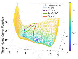
(a)

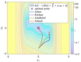
(b)

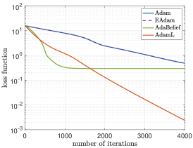
(c)

Figure 2: Three-Hump Camel Function: trajectories of the various optimizers in the contour (a) and mesh (b) plot, and the corresponding objective function values (c), when the starting point is $\mathbf{x}^{(0)}=[0,-4]^{T}$ and after $4000$ iteration steps.

Figure 2 shows the trajectories of the various optimizers in the mesh plot, contour map, and their objective function values, with the starting point $\mathbf{x}^{(0)}=[0,-4]^{T}$. Only AdamL converges to the global optimum; the other optimizers lead $\mathbf{x}^{(k)}$ to a local optimum. It can be seen from Figure 2a that the gradient and curvature near the local optima are small, which is very similar to the region of $x_{7}$, $x_{8}$, and $x_{9}$ in Figure 1b. From Figures 2a and 2b, it can be seen that the gradients and curvatures around the global optimum are larger than those around the other local optima. As discussed in subsection 2.3, Adam and EAdam take large updating steps in the direction of small gradients, whereas AdaBelief takes large updating steps in the presence of small curvatures. From Figures 2b and 2c, it can be observed that the trajectories of Adam and EAdam are identical, which implies that the accumulated $\varepsilon$ in the second moment estimate of EAdam does not affect the convergence behavior in this study. By considering the loss function values, when the gradients are small and loss function values are large, the AdamL optimizer takes large updating steps in the directions that lead to a decrease in the loss function. This explains why, for this starting point, AdamL is the only method that converges to the global optimum.

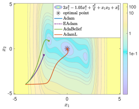
(a)

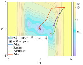
(b)

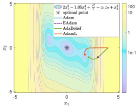
(c)

Figure 3: Three-Hump Camel Function: trajectories of different optimizer in the contour plot when the starting points are $\mathbf{x}^{(0)}=[-4,-4]^{T}$ (a), $\mathbf{x}^{(0)}=[4,4]^{T}$ (b) and $\mathbf{x}^{(0)}=[4,0]^{T}$ (c), after $4000$ iteration steps.

In Figure 3, we repeat the experiment with different starting points, i.e., $\mathbf{x}^{(0)}=[-4,-4]^{T}$ (Figure 3a), $\mathbf{x}^{(0)}=[4,4]^{T}$ (Figure 3b) and $\mathbf{x}^{(0)}=[4,0]^{T}$ (Figure 3c). In all cases, the convergence speed of the Adabelief optimizers is higher than that of Adam and EAdam, as the former takes into account the curvature of the function. We remark that AdamL performs better than its competitors in all tests by either finding the global optimum or obtaining the smallest values for the objective function.

4.2 Rosenbrock function

For the minimization of the Rosenbrock function, we choose the same settings as those applied in subsection 4.1 for adaptive optimizers ($\eta=10^{-3}$). Additionally, we also run GD with momentum, to showcase that the AdamL consistently employs its Non-Adaptive Mode. In the use of GD with momentum, we apply two different settings. In the first setup, a constant $\eta=10^{-4}$ is used, to maintain monotonicity. In the second scenario, we manually increase the value of $\eta$ from $\eta=10^{-4}$ to $\eta=10^{-3}$ when $\mathbf{x}$ reaches the long and narrow flat valley of the Rosenbrock function. Specifically, $\eta$ is increased by a factor of 10 when $f<1$. Empirically, we observe that choosing $\eta=10^{-3}$ for the initial step of GD causes divergence.

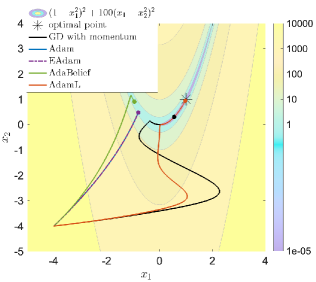
(a)

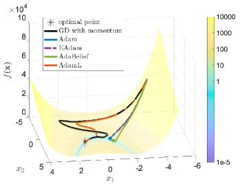
(b)

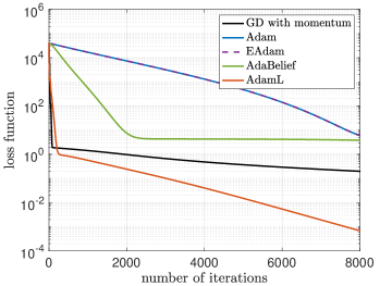
(c)

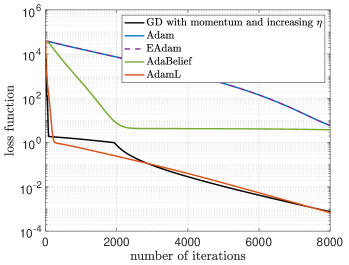
(d)

Figure 4: Rosenbrock function: trajectories of different optimizers in the contour (a) and mesh (b) plot, the corresponding objective function values when $\eta$ is constant (c), and increasing $\eta$ by a factor of 10 in GD with momentum (d), when $\mathbf{x}^{(0)}=[-4,-4]^{T}$ and after $8000$ iteration steps.

Figures 4a and 4b show the trajectories of GD with momentum with constant $\eta=10^{-4}$ and various adaptive optimizers, including Adam, EAdam, AdaBelief, and AdamL, in both contour and mesh plots, respectively. Additionally, Figure 4c depicts the corresponding objective function values after 8000 iteration steps. In Figure 4d, we report the results of GD with momentum with $\eta$ increasing from $\eta=10^{-4}$ to $\eta=10^{-3}$ when $f<1$. In Figure 4a, we see that different optimizers cause $\mathbf{x}^{(k)}$ to update in different directions. In particular, we note that the EAdam and AdaBelief optimizers update in a direction that is almost aligned with that of the Adam optimizer. This suggests that the Adaptive Mode is activated in EAdam and AdaBelief. Furthermore, the Adam and EAdam optimizers take larger steps in the directions characterized by small gradients, whereas Adabelief favors larger steps in directions where the curvatures are shallow. Therefore, they quickly reach the narrow and flat valley. From Figure 4a, we see that GD with momentum and AdamL force $\mathbf{x}^{(k)}$ to update in a similar direction, suggesting that the Non-Adaptive Mode is activated in AdamL. However, from Figures 4a and 4c, it is evident that the convergence rates of AdamL and GD with momentum are different when $\mathbf{x}^{(k)}$ reaches the narrow valley near the optimum. When manually increasing $\eta$ by a factor of 10 in GD with momentum, as shown in Figure 4d, the convergence rates of AdamL and GD with momentum become comparable. This implies that AdamL always uses the Non-adaptive updating strategy. However, as it is discussed in subsection 2.3 when the Non-Adaptive Mode is activated in AdamL, the inclusion of objective function values in the second moment estimate results in an increasing stepsize as the objective function value decreases. Consequently, AdamL obviates the need for manually increasing stepsize, unlike GD with momentum, and attains faster convergence in comparison to GD with a constant stepsize.

4.3 CNNs for image classification

In this section, we compare the performances of the various optimizers in image classification problems by training some common types of convolutional neural networks (CNNs), i.e., VGG11, ResNet18, and DenseNet121, on the CIFAR10 and CIFAR100 datasets. All these CNNs use the softmax activation function in the output layer and optimize a multi-class cross-entropy loss function using different optimizers during backward propagation. For a detailed structure of these CNNs, see (Simonyan and Zisserman, 2015; He et al., 2016; Huang et al., 2017). We apply the default setting of Adam, recommended in (Kingma and Ba, 2014), for all the optimizers, i.e., $\beta_{1}=0.9$, $\beta_{2}=0.999$, $\eta=0.001$, and $\varepsilon=10^{-8}$.

To appropriately choose the function $\ell^{(k)}$ and the value of $\varphi$ in the AdamL optimizer, we look at the range of the objective function values for these CNNs. Because of the use of the softmax activation function and the multi-class cross-entropy loss function, the loss function values are non-negative, with the optimal value close to $0$, i.e., $f^{*}\approx 0$. Additionally, the typical maximum values of the loss function, observed when optimizing these CNNs, are around $1$. In view of these remarks, we set $\ell^{(k)}=f(\mathbf{x}^{(k)})$ for all the experiments contained in this subsection. Additionally, the loss function values vary depending on the network architectures and training datasets. When the network architecture is not sufficiently complex to effectively represent the features in the training dataset, the resulting minimum value of the loss function will often be significantly distant from zero. For example, when comparing VGG11 to ResNet18 and DenseNet121 on CIFAR10 at the same iteration, VGG11 may yield higher loss function values (cf. (Zhuang et al., 2020, Fig. 1 in Appendix E)). In this case, a large value $\varphi$ is necessary to ensure that the minimum loss function approaches the optimal value as closely as possible. This choice facilitates a smooth transition between the Non-Adaptive and Adaptive modes within the AdamL optimizer. As discussed after Eq. 8, $\varphi$ should also be chosen such that $(\ell^{(k)})^{\varphi}$ reacts sensitively as $\ell^{(k)}$ approaches $0$. This requires choosing an appropriate value for $\varphi$: large enough for VGG11, but not too big for ResNet18 and DenseNet121. For this reason, we define $\varphi$ as a function of the training error $e_{\mathrm{train}}$ (%) in the exponent; more precisely we set $\varphi=\max\{4,4+\log_{10}(e_{\mathrm{train}})\}$. With this choice, $\varphi$ is set to $4$ when the training error is $1\%$ or lower and a higher value of $\varphi$ when the training error is larger than $1\%$.

In (Luo et al., 2019; Zhuang et al., 2020; Yuan and Gao, 2020), to improve the training accuracy, the learning rates $\eta$ of the optimizers are manually reduced by a factor of $0.1$ when the training accuracy reaches a steady state. Instead of manually decreasing the value of $\eta$, the AdamL optimizer uses $\gamma$ to control the transition from SGD to the adaptive method. As it is stated in subsection 2.4, a larger value of $\gamma$ postpones the shift to the Adaptive Mode. We start with the default value $\gamma=1$ and monitor the curve of training accuracy until we observe that it becomes a steady state. If it reaches a steady state too early, we increase $\gamma$ by a factor of 10 and observe the effect on training accuracy. If the change is minimal, we consider larger increments, such as multiplying $\gamma$ by $50$ or $100$. If we notice a significant improvement in training accuracy, we choose to make smaller adjustments to $\gamma$, typically multiplied by a factor less than $10$. This way, we generate the results associated with AdamL in Figures 5 and 6; the latter illustrates the convergence behavior of the method for different values of $\gamma$ when training CNNs on the CIFAR10 and CIFAR100 datasets.

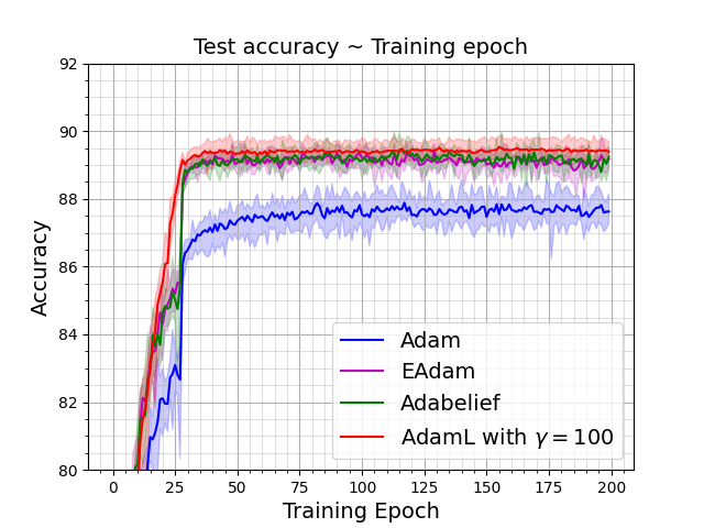
(a) VGG11 on CIFAR10

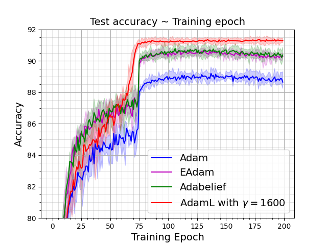
(b) VGG11 on CIFAR10

(c) ResNet18 on CIFAR10

(d) ResNet18 on CIFAR10

(e) DenseNet121 on CIFAR10

(f) DenseNet121 on CIFAR10

Figure 5: Mean values of testing accuracy of CNNs over 5 independent runs on CIFAR10 dataset trained using Adam, Adabeleif, and AdamL with early (left column) and late (right column) decay epoch.

(a) VGG11 on CIFAR100

(b) VGG11 on CIFAR100

(c) ResNet18 on CIFAR100

(d) ResNet18 on CIFAR100

(e) DenseNet121 on CIFAR100

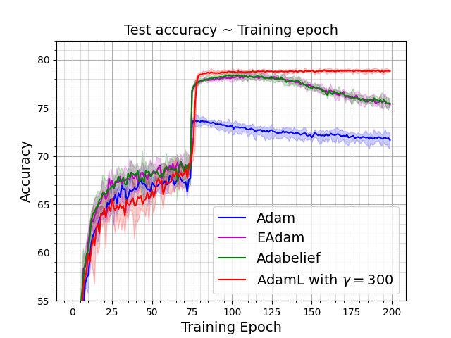
(f) DenseNet121 on CIFAR100

Figure 6: Mean values of testing accuracy of CNNs over 5 independent runs on CIFAR100 dataset trained using Adam, Adabelief, and AdamL with early (left column) and late (right column) decaying epoch.

The performances of AdamL are compared with those obtained by running Adam, EAdam, and AdaBelief and manually reducing the learning rate in the same training epoch when AdamL switches from the Non-Adaptive to the Adaptive mode. Figures 5 and 6 show comparison of testing accuracies achieved by various optimizers for VGG11, ResNet18, and DenseNet121 when trained on the CIFAR10 and CIFAR100 datasets, respectively. It can be observed that the AdamL optimizer demonstrates higher testing accuracies and faster convergence compared to other optimizers when training VGG11. In the cases of ResNet18 and DenseNet121, the highest testing accuracies obtained by EAdam, AdaBelief, and AdamL are very similar. When decreasing the learning rate at the early stage of training, both EAdam and AdaBelief show unstable convergence, as defined in (Ahn et al., 2022). Additionally, these two optimizers demonstrate similar testing accuracies across all numerical tests in this subsection. Increasing the value of $\gamma$ in the AdamL optimizer improves testing accuracies across all CNNs in Figures 5 and 6, but it simultaneously leads to slower convergence. Furthermore, the Adam optimizer consistently produces the lowest testing accuracies among all the optimizers. By comparing Figures 5 and 6, we can draw a similar conclusion for CIFAR100 as we do for CIFAR10.

It is worth noting that although tuning the value of $\gamma$ for different CNNs and datasets typically involves monitoring changes in training errors, Figures 5 and 6 demonstrate that it is not necessary to postpone tuning $\gamma$ until the later stages of training. In most cases, within the first 25 training epochs, it is possible to determine if the chosen $\gamma$ is appropriate.

4.4 Experiments with generative adversarial network

Adaptive optimizers such as Adam and RMSProp are the workhorse for the training of generative adversarial networks (GANs) because training GANs with SGD often fails. Wasserstein GAN (WGAN) is modified based on GAN to improve the training stability by using the Wasserstein distance as the loss function (Arjovsky et al., 2017). A thorough comparison between the AdaBelief optimizer and other optimization methods in training WGAN and its improved version with gradient penalty (WGAN-GP) has been carried out in (Zhuang et al., 2020, Fig.6). To ensure a fair comparison, we first replicate the same experiments using AdaBelief and, subsequently, evaluate the performances of the EAdam and AdamL optimizers based on the code published in the GitHub repository. For a detailed description of the network structure, see (Zhuang et al., 2020, Tab. 1 in Appendix F). To observe the convergence behavior of each optimizer, the Fréchet Inception Distance (FID) (Heusel et al., 2017, (6)) between the fake images and the real dataset is computed every 20 epochs by generating 64,000 fake images from random noise. Note that the FID score is a common metric to capture the similarity of generated images to real ones, and is considered to have consistency with increasing disturbances and human judgment (Heusel et al., 2017). In both WGAN and WGAN-GP, the settings for Adabelief and EAdam are consistent with those in (Zhuang et al., 2020, Fig. 6), i.e., $\beta_{1}=0.5$, $\beta_{2}=0.999$, $\varepsilon=10^{-12}$, $\eta=2\cdot 10^{-4}$. We clip the weight of the discriminator to a range of $-0.01$ to $0.01$ in the WGAN experiment and we set the weight for the gradient penalty to $10$ in the case of WGAN-GP, to be consistent with the settings in (Zhuang et al., 2020).

As discussed in subsection 2.4, the generator aims to minimize the Wasserstein distance (Arjovsky et al., 2017, Eq. (2)), while the discriminator/critic aims to maximize it. Additionally, the parameters of the discriminator are updated more frequently compared to that of the generator (cf. (Arjovsky et al., 2017, Algorithm. 1)), and this yields a more accurate approximation of the Wasserstein distance (Arjovsky et al., 2017, Sec. 3). Therefore, we only apply AdamL for updating the parameters of the discriminator. As for the generator, we set $\ell^{(k)}=1$ for all $k$, which is equivalent to the EAdam optimizer. In the context of training WGAN with AdamL, we present the results obtained based on two strategies for defining $\ell^{(k)}$. The first approach employs AdaBelief to estimate the output of the discriminator given fake generated data, and subsequently defining $\ell^{(k)}$ as $\tfrac{f(\mathbf{x}_{f}^{(k)})-f_{\min}}{f_{\max}-f_{\min}}$. The second strategy uses Algorithm 2 for the automated adjustment of $\ell^{(k)}$.

Estimating $\ell^{(k)}$ using Adabelief. In the training of WGAN, the discriminator tries to maximize its output given real training data, denoted as $f(\mathbf{x}_{r}^{(k)})$, and minimizes its output given fake generated data, denoted as $f(\mathbf{x}_{f}^{(k)})$, simultaneously. We use the output of the discriminator given fake generated data as our loss function values in the AdamL optimizer. Empirically, we find that when using the AdaBelief optimizer, the output of the discriminator given fake generated data typically falls within the range of $0.34\leq f(\mathbf{x}_{f}^{(k)})\leq 0.6$. Therefore, by scaling the loss by using the scheme $\ell^{(k)}=\tfrac{f(\mathbf{x}_{f}^{(k)})-0.32}{0.2}$, the updating stepsize will gradually decrease once the loss falls below $0.52$; this ensures $\ell^{(k)}\geq 0.1$. Numerically, we find that choosing $\gamma=1$ and reducing the updating stepsize by a factor of $100$ (by setting $\varphi=4$), is good enough for training WGANs in our experiments. Similarly, we set $\ell^{(k)}=\tfrac{f(\mathbf{x}_{f}^{(k)})+100}{100}$, $\gamma=1$, and $\varphi=4$ in the experiment of WGAN-GP.

In the experiments presented in (Zhuang et al., 2020, Fig.6), the AdaBelief optimizer performs better than the other Adam’s variants and SGD, as it yields the lowest average FID score in both WAGN and WGAN-GP. Therefore, here we only compare with the results obtained by AdaBelief and EAdam (not considered in Zhuang et al. (2020)). We provide the averaged FID scores along with their maximum and minimum values from 5 independent simulations in Figure 7 and summarize their detailed values and the $95\%$ confidence intervals in Table 3. We remark that in the training of WGAN, the AdamL optimizer yields the fastest convergence and lowest FID scores. In particular, the Adabelief optimizer yields an average FID score of approximately $82.23$ by the 100th training epoch. However, with the AdamL optimizer, an analogous value of $82.71$ can be attained in just 20 training epochs. After conducting 100 training epochs, the AdamL optimizer achieves an average FID score of $60.4$. Additionally, when comparing its performance to EAdam and AdaBelief, the AdamL optimizer exhibits the smallest deviation. Conversely, the EAdam optimizer performs the worst, yielding the highest FID score and the largest deviation.

In the training of WGAN-GP (cf. Figure 7b), AdamL does not clearly outperform its competitors as observed in the case of WGAN. WGAN-GP introduces a penalty to the loss function, ensuring that the optimal result is associated with gradients having a norm close to 1. In particular, achieving the smallest loss function value doesn’t necessarily coincide with a gradient norm approaching 1. This suggests that in WGAN-GP, using large step sizes may not be advantageous as the loss function values approach 0. However, AdamL is designed to employ a large step size as the loss function value approaches 0 and this explains the less good performance on this case study.

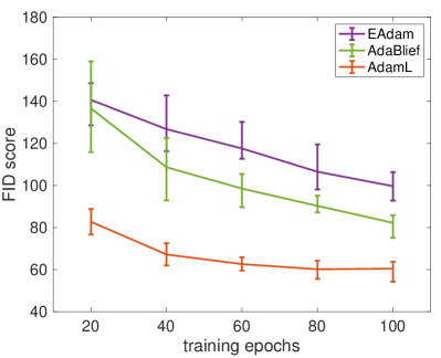
(a)

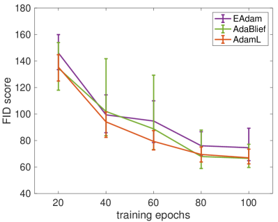
(b)

Figure 7: Mean of FID scores over 5 independent runs with an error bar of the maximum and minimum FID values for WGAN (a) and WGAN-GP (b).

Table 3: Comparison of FID score (lower is better) of training WGAN using a vanilla CNN generator on CIFAR10 between AdaBelief and AdamL; for each training epoch it shows the mean value and its $95$% ($\pm\,2\sigma$) confidence interval over 5 independent runs.

Optimizer   MM$20$th   MM$40$th   MM$60$th   MM$80$th   MM$100$th WGAN EAdam $140.6\pm 20.1$ $126.8\pm 20.9$ $117.6\pm 14.4$ $106.5\pm 16.5$ $99.7\pm 12.5$ AdaBelief $136.6\pm 32.5$ $108.7\pm 26.2$ $\phantom{1}98.5\pm 13.4$ $\phantom{1}90.3\pm\phantom{1}6.1$ $82.2\pm\phantom{1}8.3$ AdamL $\phantom{1}82.7\pm 10.7$ $\phantom{1}67.2\pm\phantom{1}8.9$ $\phantom{1}62.6\pm\phantom{1}6.0$ $\phantom{1}60.2\pm\phantom{1}7.0$ $60.4\pm\phantom{1}7.4$ WGAN-GP EAdam $146.1\pm 19.1$ $\phantom{1}99.4\pm 20.2$ $\phantom{1}94.7\pm 24.7$ $\phantom{1}76.0\pm 12.7$ $74.6\pm 16.8$ AdaBelief $134.6\pm 28.5$ $101.9\pm 38.2$ $\phantom{1}88.8\pm 37.6$ $\phantom{1}67.9\pm 17.8$ $66.5\pm 11.8$ AdamL $135.4\pm 12.8$ $\phantom{1}94.1\pm 11.0$ $\phantom{1}79.3\pm 10.0$ $\phantom{1}69.5\pm\phantom{1}8.1$ $67.0\pm\phantom{1}6.5$

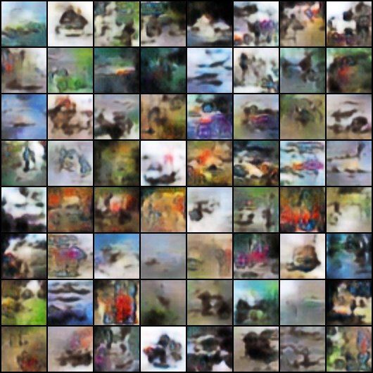
(b)

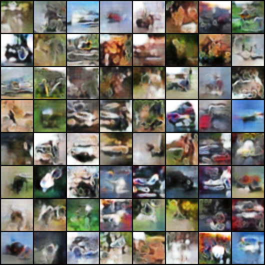
(c)

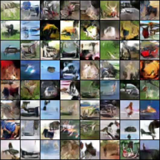
(d)

Figure 12: Real images (a) and samples from WGAN trained using EAdam (b), AdaBelief (c) and AdamL (d) at 40th training epoch.

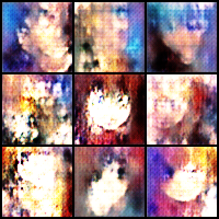
(b) Adam at $20$th

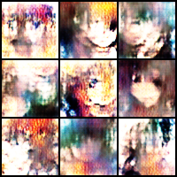
(c) EAdam at $20$th

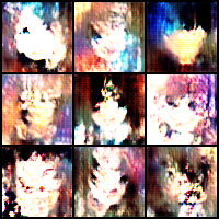
(d) AdaBelief at $20$th

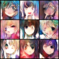
(e) AdamL at 20th

(f) Adam at 80th

(g) EAdam at 80th

(h) AdaBelief at 80th

(i) AdamL at 80th

(j) Adam at 150th

(k) EAdam at 150th

(l) AdaBelief at 150th

(m) AdamL at 150th

Figure 13: AnimeFaces Dataset: Real images (a) and Generated samples from WGAN trained using EAdam, AdaBelief, and AdamL at different training epochs.

In Figure 12 of section A, we compare the fake samples generated from the WGAN trained using the AdaBelief and AdamL optimizers after $40$ training epochs. Notably, the samples produced with AdamL exhibit significantly clearer images compared to those generated with AdaBelief, which are still slightly blurred. For a more intuitive visualization, we conduct training of the WGAN on the Anime Faces dataset. We remark that the parameters of AdamL are chosen in accordance with those used for CIFAR10. In section A, we illustrate the fake images generated by the WGAN, trained with different optimization algorithms, at the 20th, 80th, and 150th training epochs (cf. Figure 13). It can be seen that at the 20th training epoch, the generated images obtained by Adam, EAdam, and AdaBelief demonstrate a deficiency in clarity and manifest distorted facial features. Conversely, the images generated with the AdamL optimizer exhibit better quality. With an increasing number of iterations, the quality of the generated images improves further. Remarkably, even at the 40th training epoch, the images produced by AdamL already show better quality than those generated by other optimizers at the 100th training epoch in terms of FID score.

Automatically estimating $\ell^{(k)}$ using Algorithm 2. Let us replicate the experiment of training WGAN on the Anime Faces dataset using Algorithm 2 and keeping the same parameter configuration, $\varphi=4$ and $\gamma=1$. Figure 8 shows the mean FID scores over 5 independent runs, along with error bars indicating the maximum and minimum values. It can be observed that when using the AdamL optimizer, employing Algorithm 2 to automatically estimate $\ell^{(k)}$ yields FID scores similar to those obtained when $f$ is known (estimated using AdaBelief). Also, the FID scores obtained using Adam, EAdam, and AdaBelief show this behavior. Typically, the FID scores obtained with these optimizers are around $97$ with 150 training epochs, while AdamL achieves a similar FID score of approximately $99$ with only $60$ training epochs.

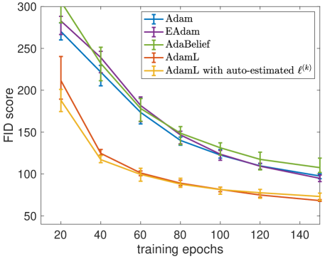
Figure 8: AnimeFaces Dataset: Mean of FID scores over 5 independent runs with error bars of the maximum and minimum FID values for WGAN.

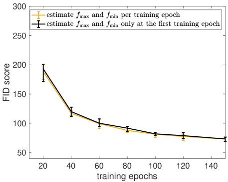
Figure 9: AnimeFaces Dataset: Mean of FID scores over 5 independent runs with an error bar of the maximum and minimum FID values for WGAN.

In subsection 2.4, we remark that when training a GAN, it is common to observe significant fluctuations in the discriminator’s output during the first training epoch. Consequently, Algorithm 2 computes $\ell^{(k)}$ only based on the estimation of $f_{\min}$ and $f_{\max}$ in the first training epoch. Here, we demonstrate that similar results can be achieved as in Algorithm 2 when training a WGAN by computing $\ell^{(k)}$ based on the estimation of $f_{\min}$ and $f_{\max}$ during each training epoch. We replicate the experiments presented in Figure 8 using the AdamL optimizer, with updates to $f_{\min}$ and $f_{\max}$ being made at the end of each training epoch. The results shown in Figure 9 are very close to those obtained by applying Algorithm 2.

4.5 LSTM for language modeling

In this last numerical study, we consider the language modeling task that consists of training LSTM models with 1, 2, and 3 layers on the Penn Treebank dataset. These experiments are conducted based on the code available on the GitHub repository. In line with the evaluations of EAdam and AdaBelief (Yuan and Gao, 2020; Zhuang et al., 2020), the perplexity is employed to measure the performance of all algorithms under comparison. Note that perplexity is a commonly used metric for assessing the performance of a language model, with lower values indicating better performance (Chen and Goodman, 1999).

For all the experiments of LSTM, the settings for AdaBelief, EAdam, and AdamL are aligned with those in (Zhuang et al., 2020), i.e., $\beta_{1}=0.9$, $\beta_{2}=0.999$, $\varepsilon=10^{-12}$ and $\eta=0.01$. Note that in (Zhuang et al., 2020), to achieve the best result of AdaBelief, a learning rate of $0.001$ was chosen for 1-layer LSTM, and a learning rate of $0.01$ was used for 2 and 3-layer LSTM. In particular with $\eta=0.001$, the lowest test perplexity of 1-layer LSTM obtained by AdaBelief is approximately $84.2$ (Zhuang et al., 2020, Fig. 5), which is still higher than the result of AdamL with $\eta=0.01$, i.e., $81.7$ in Table 4.

Estimating $\ell^{(k)}$ using Adam. Observing the results obtained by Adam, we found that the objective function values of $1$, $2$, and $3$-layer LSTM change very mildly; more precisely, in the first 200 training epochs, it ranges between $9$ to $3$. To ensure that the objective function has some part larger than 1 and some part smaller than 1, we normalize it by dividing it by 6, i.e., $\ell^{(k)}=\ell(f(\mathbf{x}^{(k)}))=\frac{1}{6}\,f(\mathbf{x}^{(k)}$. Additionally, we set $\varphi=4$ to improve the sensitivity of $(\ell^{(k)})^{\varphi}$ to the changes in $\ell^{(k)}$, causing the value of $(\ell^{(k)})^{\varphi}$ to approach $0$ as $\ell^{(k)}$ decreases. We empirically find that setting $\gamma=0.5$ yields the best performance for AdamL in the case of a 1-layer LSTM, while for 2 and 3-layer LSTMs, the optimal value appears to be $\gamma=1$.

We manually decrease the learning rate by a factor of $0.1$ at different training epochs for all the optimizers. The corresponding average perplexities over 5 independent simulations are presented in Table 4. Note that in the experiment of LSTM, we lose AdamL’s benefit of not manually adjusting the learning rate to improve performance. In Table 4, the optimizers that produce the highest perplexities are highlighted in red and the ones that yield the lowest ones are marked in bold. As can be observed, the EAdam optimizer slightly outperforms the AdaBelief optimizer in the training of LSTM models, while the AdamL optimizer always results in the lowest perplexities for all the experiments.

Table 4: Mean value of test perplexity and its maximum deviation from its mean value over 5 independent simulations (lower is better) of 1, 2, and 3-layer LSTM on Penn Treebank.

	learning rate decay epoch	Adam	EAdam	AdaBelief	AdamL
1-layer	1$75$th and $150$th	$89.4$	$90.0$	$91.3$	$\mathbf{82.1}$
	$100$th and $145$th	$91.3$	$91.6$	$93.3$	$\mathbf{81.7}$
2-layer	$\phantom{1}75$th and $150$th	$67.1$	$66.5$	$66.9$	$\mathbf{66.0}$
	$100$th and $145$th	$67.0$	$66.4$	$66.7$	$\mathbf{65.4}$
3-layer	$\phantom{1}75$th and $150$th	$64.6$	$61.9$	$62.1$	$\mathbf{61.1}$
	$100$th and $145$th	$64.4$	$61.0$	$61.2$	$\mathbf{60.5}$

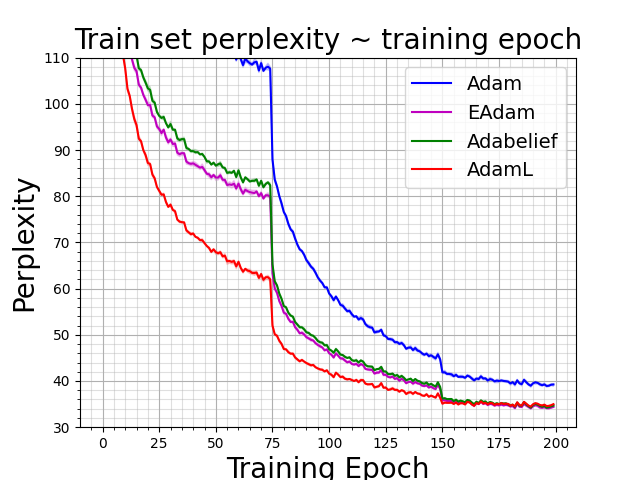
(a)

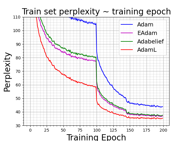
(b)

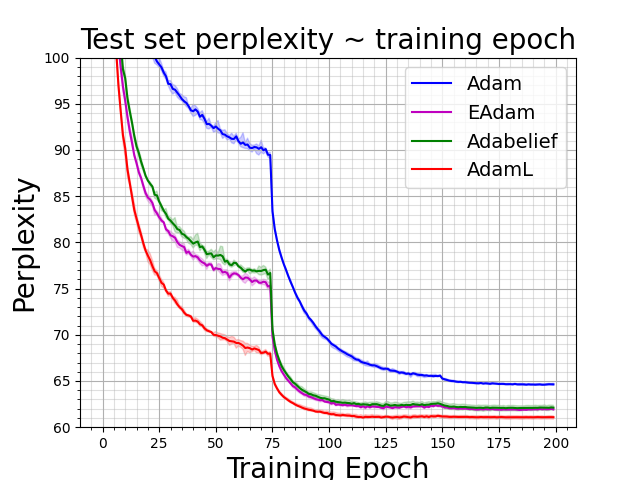
(c)

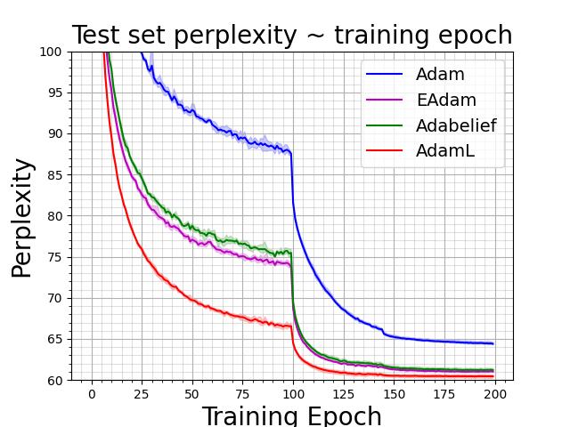
(d)

Figure 10: Mean values of training (top row) and testing (bottom row) perplexities and their maximum deviation from the mean value over 5 independent simulations (lower is better) of 3-layer LSTM on Penn Treebank.

Figure 10 shows the mean values of train and test perplexities, along with their maximum deviations, from 5 independent simulations of the 3-layer LSTM. Notably, the improvement in convergence achieved by the second learning rate decrease in the AdamL optimizer appears to be minimal. After the first learning rate reduction, the testing perplexity obtained by AdamL is already lower than that achieved by other optimizers even when they undergo two learning rate decreases. Overall, the AdamL optimizer achieves both the fastest convergence and good accuracy compared to the other adaptive methods.

Automatically estimating $\ell^{(k)}$ using Algorithm 2. To study the effectiveness of Algorithm 2, we repeat the same experiments for training a 2-layer and 3-layer LSTMs on the Penn Treebank dataset using the estimation strategy in Algorithm 2. Figure 11 shows the mean values of training and testing perplexities over 5 independent runs and their corresponding maximum deviations. We see that before triggering the reduction of the initial learning rate, the convergence is slower in comparison to the strategy that relies on the knowledge of $\ell^{(k)}$ obtained with an initial training phase with the Adam optimizer. On the other hand, after the second reduction in the learning rate, the training and testing perplexities obtained with these two strategies become quite similar.

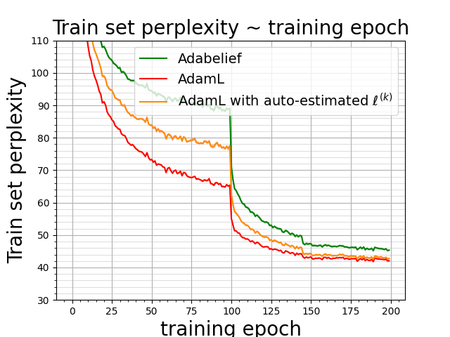
(a)

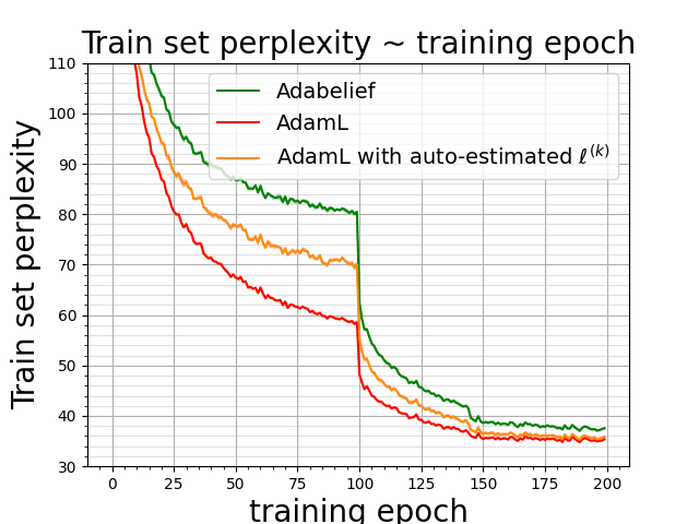
(b)

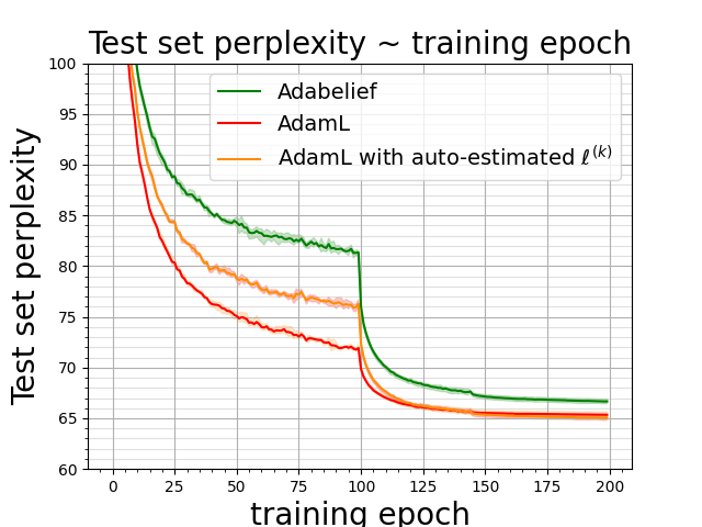
(c)

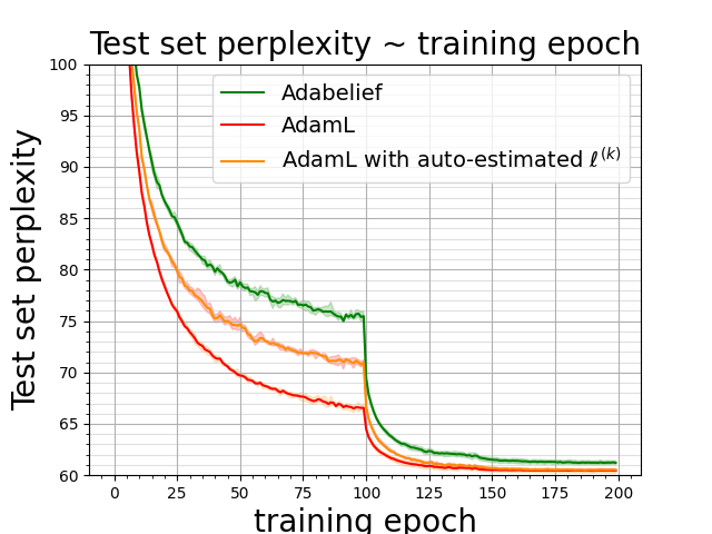
(d)

Figure 11: Mean values of training (top row) and testing (bottom row) perplexities and their maximum deviation from the mean value over 5 independent simulations (lower is better) of 2-layer ((a) and (c)) and 3-layer ((b) and (d)) LSTM on Penn Treebank.

5 Conclusion

We have proposed a new variant of Adam that takes into account the loss function, namely AdamL. We have provided sufficient conditions for the monotonicity and linear convergence of AdamL and other Adam’s variants. Extensive numerical tests on both benchmark examples and neural network case studies have been presented to compare AdamL with some leading competitors.

Overall, we found that AdamL performs better than the other Adam’s variants in various training tasks. For instance, it exhibits either faster or more stable convergence when applied to the training of convolutional neural networks (CNNs) for image classification and for training generative adversarial networks (WGANs) using vanilla CNNs. In the context of training CNNs for image classification, AdamL stands out from other variants of Adam and eliminates the need for manually adjusting the learning rate in the later stages of the training. When training WGANs, we have introduced two primary approaches for implementing AdamL. The first approach involves pre-training the WGANs using Adam or another optimizer, and then estimating $\ell^{(k)}$ based on the maximum and minimum cost function values observed during the pre-training process. Alternatively, Algorithm 2 presents a method for automatically estimating $\ell^{(k)}$, that yields comparable results with the first approach. Notably, for both approaches, the convergence speed of AdamL is more than twice as fast as that achieved by leading competitors such as Adam, AdaBelief, and EAdam. Finally, AdamL also demonstrates improved performance in training LSTMs for language modeling tasks. Despite the requirement for additional hyperparameters when compared to Adam, EAdam, and AdaBelief, we have shown that the choice of these hyperparameters is relatively consistent. For instance, values like $\gamma=1$ and $\varphi=4$ are employed in the training of both WGANs and LSTMs, and the scaling function can be automatically estimated using Algorithm 2. The potential of AdamL in other training scenarios remains a subject for future investigation.

A Numerical experiments on WGANs

(a)

(a) Real Images

References

- Ahn et al. (2022) K. Ahn, J. Zhang, and S. Sra. Understanding the unstable convergence of gradient descent. In International Conference on Machine Learning, pages 247–257. PMLR, 2022.
- Arjovsky et al. (2017) M. Arjovsky, S. Chintala, and L. Bottou. Wasserstein generative adversarial networks. In Proceedings of the 34th International Conference on Machine Learning, Aug 2017.
- Cao et al. (2020) L. Cao, X. Sun, Z. Xu, and S. Ma. On the convergence of a class of adam-type algorithms for non-convex optimization. In International Conference on Learning Representations, 2020.
- Chen and Goodman (1999) S. F. Chen and J. Goodman. An empirical study of smoothing techniques for language modeling. Computer Speech & Language, 13(4):359–394, 1999. ISSN 0885-2308. doi: https://doi.org/10.1006/csla.1999.0128.
- Duchi et al. (2011) J. Duchi, E. Hazan, and Y. Singer. Adaptive subgradient methods for online learning and stochastic optimization. Journal of machine learning research, 12(7), 2011.
- Ghadimi and Lan (2013) S. Ghadimi and G. Lan. Stochastic first-and zeroth-order methods for nonconvex stochastic programming. SIAM Journal on Optimization, 23(4):2341–2368, 2013.
- Ghadimi et al. (2016) S. Ghadimi, G. Lan, and H. Zhang. Mini-batch stochastic approximation methods for nonconvex stochastic composite optimization. Mathematical Programming, 155(1-2):267–305, 2016.
- He et al. (2016) K. He, X. Zhang, S. Ren, and J. Sun. Deep residual learning for image recognition. In the IEEE conference on computer vision and pattern recognition, pages 770–778, 2016.
- Heusel et al. (2017) M. Heusel, H. Ramsauer, T. Unterthiner, B. Nessler, and S. Hochreiter. Gans trained by a two time-scale update rule converge to a local nash equilibrium. Advances in neural information processing systems, 30, 2017.
- Hoffer et al. (2017) E. Hoffer, I. Hubara, and D. Soudry. Train longer, generalize better: closing the generalization gap in large batch training of neural networks. Advances in neural information processing systems, 30, 2017.
- Huang et al. (2017) G. Huang, Z. Liu, L. Van Der Maaten, and K. Q. Weinberger. Densely connected convolutional networks. In the IEEE conference on computer vision and pattern recognition, pages 4700–4708, 2017.
- Keskar and Socher (2017) N. S. Keskar and R. Socher. Improving generalization performance by switching from adam to sgd. arXiv preprint arXiv:1712.07628, 2017.
- Kingma and Ba (2014) D. P. Kingma and J. Ba. Adam: A method for stochastic optimization. arXiv preprint arXiv:1412.6980, 2014.
- Luo et al. (2019) L. Luo, Y. Xiong, Y. Liu, and X. Sun. Adaptive gradient methods with dynamic bound of learning rate. In International Conference on Learning Representations, New Orleans, Louisiana, May 2019.
- Nemirovski et al. (2009) A. Nemirovski, A. Juditsky, G. Lan, and A. Shapiro. Robust stochastic approximation approach to stochastic programming. SIAM Journal on optimization, 19(4):1574–1609, 2009.
- Nguyen et al. (2019) P. Nguyen, L. Nguyen, and M. van Dijk. Tight dimension independent lower bound on the expected convergence rate for diminishing step sizes in sgd. Advances in Neural Information Processing Systems, 32, 2019.
- Qian (1999) N. Qian. On the momentum term in gradient descent learning algorithms. Neural networks, 12(1):145–151, 1999.
- Reddi et al. (2018) S. J. Reddi, S. Kale, and S. Kumar. On the convergence of adam and beyond. In International Conference on Learning Representations, 2018.
- Robbins and Monro (1951) H. Robbins and S. Monro. A stochastic approximation method. The annals of mathematical statistics, pages 400–407, 1951.
- Simonyan and Zisserman (2015) K. Simonyan and A. Zisserman. Very deep convolutional networks for large-scale image recognition. In 3rd International Conference on Learning Representations, 2015.
- Tieleman and Hinton (2012) T. Tieleman and G. Hinton. Rmsprop: Divide the gradient by a running average of its recent magnitude. COURSERA: Neural Networks for Machine Learnin, 2012.
- Wilson et al. (2017) A. C. Wilson, R. Roelofs, M. Stern, N. Srebro, and B. Recht. The marginal value of adaptive gradient methods in machine learning. Advances in neural information processing systems, 30, 2017.
- Xia et al. (2023) L. Xia, M. E. Hochstenbach, and S. Massei. On the convergence of the gradient descent method with stochastic fixed-point rounding errors under the Polyak-Lojasiewicz inequality. arXiv preprint arXiv:2301.09511, 2023.
- Yuan and Gao (2020) W. Yuan and K.-X. Gao. EAdam Optimizer: How Impact Adam. arXiv preprint arXiv:2011.02150, 2020.
- Zaheer et al. (2018) M. Zaheer, S. Reddi, D. Sachan, S. Kale, and S. Kumar. Adaptive methods for nonconvex optimization. Advances in neural information processing systems, 31, 2018.
- Zhuang et al. (2020) J. Zhuang, T. Tang, Y. Ding, S. C. Tatikonda, N. Dvornek, X. Papademetris, and J. Duncan. Adabelief optimizer: Adapting stepsizes by the belief in observed gradients. Advances in neural information processing systems, 33:18795–18806, 2020.