Wavelet Packet Power Spectrum Kullback-Leibler Divergence: A New Metric for Image Synthesis

Abstract

Current metrics for generative neural networks are biased towards low frequencies, specific generators, objects from the ImageNet dataset, and value texture more than shape. Many current quality metrics do not measure frequency information directly. In response, we propose a new frequency band-based quality metric, which opens a door into the frequency domain yet, at the same time, preserves spatial aspects of the data. Our metric works well even if the distributions we compare are far from ImageNet or have been produced by differing generator architectures. We verify the quality of our metric by sampling a broad selection of generative networks on a wide variety of data sets. A user study ensures our metric aligns with human perception. Furthermore, we show that frequency band guidance can improve the frequency domain fidelity of a current generative network.

1 Introduction

Measuring the performance of generative neural networks is both extremely important and challenging. The fid [9] has emerged as the de facto standard for comparing generative approaches for image synthesis. Indeed, fid is a very useful metric for comparing different runs of the same architecture and in such a setting reductions in fid align well with human perception [18].

fid, however, has major shortcomings when it is used to compare different architectures and only some of them can be addressed. fid highly depends on the number of data samples [3] and the Gaussian assumptions, which are required to compute fid, are not always valid [23]. It is sensitive to resizing algorithms and the implementations are not always consistent [30], which impact the reproducibility of reported fid scores [30]. For instance, Figure 1 illustrates the sensitivity of fid to tiny differences between images caused by rounding. While all three images are perceptually identical, fid shows surprisingly large differences between the images. In other words, fid might indicate a difference that does not exist. This is also important when GANs are compared with diffusion models since diffusion models clamp inputs differently, which affects the fid score as well.

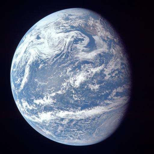
(a)

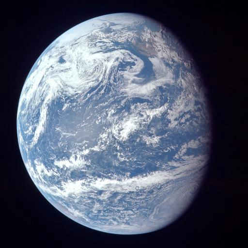
(b)

(c)

Figure 1: Illustration of fid sensitivity: The three images show Earth from space [28]. We normalized all pixel values to the interval [0,1]. While for (a) we use full precision, we rounded the values to two decimals in (b) and three decimals in (c). Although there is perceptually no difference between the three images, the rounding results in different fid values using (a) as reference. The fid is 2.12 between (a) and (b) and 0.63 between (a) and (c). In contrast, our proposed wavelet-based metric $\mathcal{D_{W}}$ is less sensitive to tiny differences with values 0.004 for (b) and 0.003 for (c).

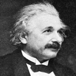
(a)

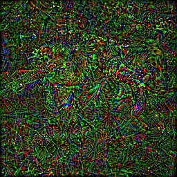
(b)

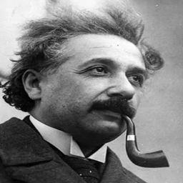
(c)

Figure 2: The images (a) and (c) depict Einstein with a bow tie and a pipe, respectively. Image (b) is a noise image that generates similar activations of InceptionV3 than (a). According to fid, (b) (fid 1.95) is more similar to (a) than (c) (fid 271.48). The large FID for (c) is caused by the pipe. Our metric $\mathcal{D_{W}}$ is more plausible and results in 3.49 for (b) and 2.74 for (c). Image source [34].

Furthermore, fid-scores are ImageNet class dependent and produce accidental distortions [18]. The fid scores improve if the evaluation set resembles ImageNet classes or if the use of ImageNet weights in generators pushes the output distribution towards ImageNet. While uninitialized random embeddings do not create an ImageNet bias [27], they do not solve the problem. Figure 2 illustrates an example where the InceptionV3 yields a bow-tie label for the left image of Figure 2 and a saxophone label for the right image. Even though both images are perceptually similar, the misclassification causes a very large fid between the left and right image. The center image shows strategic noise, optimized to produce an optimization map resembling that of Einstein with a bow tie. Even though the two images do not resemble each other, the distance between both activation maps, and thus fid, is low. In other words, similar images can have a high fid and dissimilar images can have a low fid.

In order to address the two main shortcomings of fid, namely high sensitivity to small numerical differences and dataset bias caused by the use of a pre-trained network, we propose an alternative metric based on the Wavelet Packet Transform. In contrast to a metric in the frequency domain or in the spatial domain, wavelets have the advantage that they combine both spatial and frequency information. The frequency information is important since generative neural networks have a frequency bias [5] that differs from real images. The frequency information, however, is insufficient to assess the quality of synthesized images without considering additional spatial information. Wavelets are thus a ideal representation for a metric comparing generative approaches for image synthesis.

In summary, we propose the wpskl as a quality metric for generative approaches for image synthesis, which combines spatial and frequency information. We re-evaluated several GAN and diffusion models and compare the proposed metric with fid and ssim [46] on 5 datasets. We support the experimental evaluation with a user study that underpins the usefulness of the proposed metric. Finally, we show that training with an additional wavelet packet loss reduces the frequency bias of a generative network. We will release reference implementations as a python package for future wpskl computations.

[width=0.95height=0.15]./figures/miscellaneous/activation_maps/einstein_chaplin/act_eins

(a) Einstein with bow tie

[width=0.95height=0.15]./figures/miscellaneous/activation_maps/einstein_chaplin/act_noise

(b) Strategic noise

[width=0.99height=0.163]./figures/miscellaneous/activation_maps/einstein_chaplin/act_einspipe

(c) Einstein with pipe

Figure 3: Activations from InceptionV3 for all the three images in Figure 2 before computing the fid. For visualization purposes, we reshaped the activations from $(1,2048)$ to $(32,64)$. Between images of Albert Einstein (a) and Strategic noise (b), the activations are quite similar. Whereas between (a) and (c), the activations are different. The activations from InceptionV3 are responsible for large FID between (a) and (c), and vice versa for low FID between (a) and (b).

2 Related Work

2.1 Generative Machine Learning

Prior art primarily relies on either gan or diffusion architectures. The style-gan architecture family [15, 16, 14] is among the pioneering architectures in the field. While gan allow comparatively fast inference speed, they suffer from training instabilities [2]. This difficulty motivated the search for alternative network structures. Diffusion models are emerging as an up-and-coming alternative. Recent works claim image quality comparable to gan [10]. Gaussian diffusion models as formulated by [10] are called ddpm. ddpm are Markovian processes that gradually add noise to the data in the forward process and generate images from Gaussian noise by an reverse process that requires to iterate through all steps to generate an image.

[40] reduced the number of sampling steps by introducing ddim, which rely on a deterministic non-Markovian sampling process. Furthermore, [29] proposed the use of strided sampling, which reduces the $T$ timesteps to $S$ ($S<T$) and also improves the performance by using cosine instead of linear sampling. Since the mse loss formulated in [10] does not provide information about the variance of the noise and focuses only on the mean, [29] improves the loss by adding a weighted variational lower bound to the mse loss. [7] proposed wsgm that use wavelet acceleration to speed up the diffusion process. By breaking the problem into multiple smaller sub-tasks on different scales, the fwt can speed up convergence.

In an attempt to solve the generative learning trilemma (high sample quality, diverse, and fast sampling), [49] proposed Diffusion-GAN. Diffusion-gan utilize adversarial loss terms during training and follow a ddpm sampling process. Following in the footsteps of DDGAN, [33] introduces a fwt into a UNet and trains it with a weighted combination of adversarial and mse loss. The authors report faster sampling times and high quality.

2.2 Measuring the Quality of Generated Images

Image distance metrics are a possible option to evaluate the quality of generated images. The ssim is a longstanding image distance metric [46]. The score takes luminance, contrast, and structure into account. Previous work reports ssim’s preference for blurry images [37], which disagrees with human perception. In a generative machine learning context, [38] proposed the is as a metric for image quality. Labels are found for all generated images by evaluating an inception network to compute the metric. For images with meaningful objects, the label entropy should be low. Image entropy, however, should be high. The is is independent of the statistics of the training data set. fid improves is by computing the Wasserstein distance of high-level features from true and synthetic images. Today, comparing high-level inception net features using an fid-score [9] enjoys widespread adoption. While fid captures general trends well, the literature also discusses its drawbacks. [3] found a generator-dependent architecture bias, which limits its ability to compare samples for smaller datasets with less than 50k images. Additionally, [30] found that fid is highly sensitive to resizing and compression. [23] found non-Gaussian distributions of inception features on ImageNet. The paper reports improved stability without Gaussian assumptions. While comparing Tensorflow and Pytorch implementations, [30] measured inconsistent scores due to differing resizing implementations. Finally, [16] reports fid favours texture more than shape, while humans tend to do the opposite. Generally, fid scores are hard to reproduce unless all details regarding its computation are carefully disclosed [1]. The aforementioned discussion motivates the search for additional quality metrics.

2.3 Frequency scoring for generative networks

Understanding and dealing with the tendency of current generative networks to favor low-frequency and large-scale content is a longstanding research problem [11, 35, 5, 6, 48, 52]. The tools allowing us to understand frequency bias are either Fourier or Wavelet-based. Wavelet transforms as pioneered by [24] and [4] have a solid track record in signal processing. The fwt and its cousin, the wpt, are starting to appear more frequently in deep learning architectures. Applications include cnn augmentation [47], style transfer [50], image denoising [21, 39], image coloring [20], face aging [22], video enhancement [45], face super-resolution [11], and generative machine learning [6, 7, 52, 33]. [8] uses the Fourier transform to measure the quality of human motion forecasting. [52] uses a Haar fwt to remove artifacts from generated images. [33] focuses on the Haar wavelet transform to increase inference speed of diffusion models. The vast majority of existing work is Haar based [33, 52, 20, 6, 45, 47, 50, 21]. The Haar wavelet is the simplest possible choice. [7] is a notable exception. It uses higher-order wavelets. The paper studies the integration of fwt in diffusion models with higher-order wavelets. The majority of prior art that works with wavelets employs the fwt [6, 47, 33, 50, 20, 21]. The wpt appears less frequently in the literature [45, 11, 22]. Previous use of the wpt is also typically Haar-wavelet based [45, 11].

3 Wavelet-Power Divergence Metric

The fid is the most common metric for evaluating generative models that synthesize images. It was originally proposed by Heusel et al. [9] to measure the similarity of images that are generated by a gan to real images, and it was subsequently used as a quality metric. fid is computed via

$$\text{FID}=||\mu-\mu_{w}||_{2}^{2}+Tr(\Sigma+\Sigma_{w}-2\sqrt{\Sigma\Sigma_{w}}),$$ (1)

where $(\mu,\Sigma)$ and $(\mu_{w},\Sigma_{w})$ are mean and covariance of the activations from the InceptionV3 [42] pool 3 layer for real and synthetic input images, respectively. Although fid has been very useful, it has major shortcomings, which can lead to misleading results when it is used exclusively to compare different methods. The issue that fid is biased and the bias depends on the generative model has been addressed in [3]. However, there are also other shortcomings as illustrated in Figures 1 and 2. Very small variations in the pixel values, which are not perceived by humans, can lead to different fid scores. This is illustrated in Figure 1 where pixel values are rounded differently. Although all the three images look identically, fid suggests that image (c) is more similar to image (a) than image (b). In this case, the rounding adversely affects the computation of the covariance matrices, which in turn leads to a large trace in (1). In other words, fid might indicate a difference between methods that does not exist and that is simply caused by a minor difference in rounding, mapping, or storing pixel values. Another major shortcoming has been discovered in [18] and is illustrated in Figure 2. fid suggests that (b) is more similar to (a) than (c). The left and center image pair has a small fid even though the images are not perceptually similar, but both are classified as bow-tie. The center image is the result of optimizing an initially noise input via gradient descent, such that the InceptionV3 feature maps of Figure 2 (a) and (b) resemble each other. The result is a low fid. Although (c) shows the same person in a similar pose as (a), fid is high since there is no bow tie in the image. Using InceptionV3 or any other network trained on ImageNet introduces a dataset bias towards objects that are present in the ImageNet dataset. Note that replacing ImageNet by another dataset or InceptionV3 by another network will not resolve this issue. Instead of trying to repair fid, we propose a new metric for comparing generative approaches for image synthesis, which does not have these shortcomings by design.

3.1 Wavelet-Power Divergence

In order to design a new quality metric for comparing generative approaches for image synthesis, one needs to be careful regarding the domain. Using feature spaces of trained networks is not an option as it introduces an unnecessary bias into the evaluation. Pixel-based metrics are biased towards low-frequency information and favor blurry results [37]. Fourier representations do not suffer from a low-frequency bias, but they discard spatial information. For instance, generating an object upside-down looks odd, but it will not be penalized by a metric using the Fourier representation. In order to consider not only frequencies, but also spatial information, we propose a metric based on the wpt. The wpt recursively filters input images. The transform produces a frequency band representation, which combines spatial and frequency information. The wpt computation relies on four carefully devised filters $a$, $h$, $v$, and $d$, which allow us to extract spectral information while at the same time also preserving some spatial information. We use a degree five symlet due to its relative stability and its balanced filter weights. While we provide more details regarding the wpt in the supplementary material, we focus in this section on the key aspects of the proposed wavelet packet-based quality metric.

For our metric, we first compute the normalized wavelet power spectrum of an image $I\in\mathbb{R}^{H\times W}$:

$$\mathcal{P}(\mathbf{I})_{[p,i,j]}=\frac{\mathcal{W}_{p}(\mathbf{I})^{2}_{[p,i,j]}}{\sum_{h=1}^{F_{h}}\sum_{w=1}^{F_{w}}\mathcal{W}_{p}(\mathbf{I})^{2}_{[p,h,w]},}$$ (2)

where $\mathcal{W}_{p}$ denotes the wpt. The indices $i$ and $j$ denote a wavelet packet coefficient in a wavelet packet, and $F_{h}$ and $F_{w}$ denote the packet height and width. $p$ is the index of a packet from the $P=4^{l}$ packets, where $l$ denotes the decomposition depth.

Equation (2) normalizes the wavelet packet coefficients to sum up to one, which allows a probabilistic interpretation. After having the normalized wavelet power spectra of two images $A$ and $B$ computed, we are able to measure the KL divergence:

$$\mathcal{D}(\mathbf{A},\mathbf{B}) =\frac{1}{P}\sum_{p=1}^{P}\sum_{h=1}^{F_{h}}\sum_{w=1}^{F_{w}}\Bigg{[}$$ (3)

$$\quad\mathcal{P}(\mathbf{A})_{[p,h,w]}\cdot\log\left(\frac{\mathcal{P}(\mathbf{A})_{[p,h,w]}}{\mathcal{P}(\mathbf{B})_{[p,h,w]}}\right)\Bigg{]},$$

where $P$ denotes the total number of packets.

For sets of color images, we add a single additional axis to (2) and (3), such that the batch axis additionally appears in both normalization and the computation of the KL-Divergence. We do the same for the channel dimension, which allows us to process distributions of color images. More formally, we normalize in this case via

$$\mathcal{P}_{b}(\mathbf{I})_{[b,c,p,i,j]}=\frac{\mathcal{W}_{p}(\mathbf{I})^{2}_{[b,c,p,i,j]}}{\sum_{b=1}^{B}\sum_{h=1}^{F_{h}}\sum_{w=1}^{F_{w}}\mathcal{W}_{p}(\mathbf{I})^{2}_{[b,c,p,h,w]}}$$ (4)

with $b$ as the batch index, and $c$ as channel index. Similarity,

$$\mathcal{D}_{b}(\mathbf{A},\mathbf{B}) =\frac{1}{P}\frac{1}{C}\sum_{b=1}^{B}\sum_{c=1}^{C}\sum_{p=1}^{P}\sum_{h=1}^{F_{h}}\sum_{w=1}^{F_{w}}\Bigg{[}$$ (5)

$$\quad\mathcal{P}_{b}(\mathbf{A})_{[b,c,p,h,w]}\cdot\log\left(\frac{\mathcal{P}_{b}(\mathbf{A})_{[b,c,p,h,w]}}{\mathcal{P}_{b}(\mathbf{B})_{[b,c,p,h,w]}}\right)\Bigg{]},$$

with $C$ the total number of color channels, three in our case. Since the Kullback-Leibler divergence is not symmetric, we define the wpskl between two images by

$$\mathcal{D}_{\mathcal{W}}(\mathbf{A},\mathbf{B})=\frac{1}{2}\left(\mathcal{D}_{b}(\mathbf{A},\mathbf{B})+\mathcal{D}_{b}(\mathbf{B},\mathbf{A})\right).$$ (6)

4 Wavelet-Power Divergence Loss

The wavelet packets are not only useful to define a metric, but they can also be used to train a generative network since they capture spatial and frequency information. We thus propose a wavelet packet guidance loss that measures the difference between the generated image and the target image in the wavelet space. The loss computes the mse between the wavelet packet representation of the network output $\hat{\mathbf{Y}}$ and the desired output $\mathbf{Y}$

$$\mathcal{L}_{w}(\mathbf{Y},\hat{\mathbf{Y}}) =\frac{1}{B\cdot C\cdot P\cdot F_{h}\cdot F_{w}}\Bigg{[}\sum_{b=1}^{B}\sum_{c=1}^{C}\sum_{p=1}^{P}\sum_{h=1}^{F_{h}}\sum_{w=1}^{F_{w}}$$ (7)

$$\left(\mathcal{W}_{p}(\mathbf{Y})_{[b,c,p,i,j]}-\mathcal{W}_{p}(\hat{\mathbf{Y}})_{[b,c,p,i,j]}\right)^{2}\Bigg{]}.$$

5 Experiments

We used PyTorch [31] for neural network training and evaluation. We work with the wavelet filter coefficients provided by PyWavelets [19]. We chose the PyTorch-Wavelet-Toolbox [26] software packages for GPU support. Furthermore, we employ scikit-image [43] to compute ssim scores.

5.1 Ranking current methods according to spectral power distribution

Dataset	Method	fid$\downarrow$	ssim$\uparrow$	$D_{\mathcal{W}}$$\downarrow$
CelebAHQ	DDPM [10]	-	0.277	1.37
	DDIM [40]	-	0.255	1.59
	WaveDiff [33]	5.94	0.255	1.35
	DDGAN [49]	7.64	0.258	1.33
	StyleSwin [52]	3.25	0.275	1.35
	StyleGAN2 [15]	-	0.253	1.35
Churches	DDPM [10]	7.89	0.001	1.66
	DDIM [40]	10.58	0.007	1.85
	WaveDiff [33]	5.06	0.010	1.63
	StyleSwin [52]	2.95	0.005	1.63
	StyleGAN2 [15]	3.86	0.009	1.67
Bedrooms
	DDPM [10]	4.90	0.011	1.46
	DDIM [40]	6.62	0.007	1.75
ImageNet	Imp. Diff. (Hybrid) [29]	19.2	0.011	1.87
	Imp. Diff. (VLB) [29]	40.1	0.009	1.93
	Diffusion Transformer [32]	3.43	0.076	1.81
CIFAR10	DDPM [10]	3.17	0.013	1.66
	DDIM [40]	4.04	0.011	1.74
	Imp. Diff. (Hybrid) [29]	3.19	0.016	1.69
	Imp. Diff. (VLB) [29]	11.47	0.012	1.73
	WaveDiff [33]	4.01	0.011	1.68
	DDGAN [49]	3.75	0.012	1.68
	StyleGAN2 [15]	2.32	0.012	1.69

Table 1: Comparing recent generative models using fid, ssim, and wpskl. We use 50k samples for CIFAR10, 10k samples for ImageNet, and 30k samples for all other datasets. The default image size is 32 for CIFAR10, 64 for ImageNet, and 256 for CelebAHQ, Churches, and Bedrooms. Papers with - do not report an fid on all datasets we consider here. For a fair comparison, all Diffusion Transformer images have been downsampled to 64 by 64 pixels using bilinear interpolation.

To understand the spectral qualities of existing generative methods for image synthesis, we evaluated various diffusion and GAN models across a wide range of datasets such as CIFAR10 [17], CelebAHQ [13], the Church and Bedroom subsets of the lsun dataset[51], and finally ImageNet [36]. For the evaluation, we used the diffusion approaches ddpm [10], ddim [40], Improved Diffusion [29], WaveDiff [11], Diffusion Transformer [32], as well as the GAN approaches DDGAN [49], StyleGAN2 [15], StyleSwin [52], and WSGM [7]. For all approaches, we used the publicly available code and compare the unconditionally generated images to the respective original dataset by computing wpskl and ssim [46]. Table 1 lists the new numbers alongside fid-scores from the literature. For CIFAR10, we use 50K images to evaluate both metrics. The ImageNet numbers are computed with 10K images as described in [29]. For CelebAHQ and LSUN we work with 30K images.

For diffusion models, we find that ddim’s sampling speed improvements come with a quality loss most of the time. The loss is apparent when comparing ddim’s scores to ddpm’s. On CIFAR10, this effect is visible for both fid and wpskl. In comparison to gan, diffusion models do slightly better in the wavelet space, with ddpm being the best-performing method. Cars, birds, cats, dogs, frogs, horses, ships, and trucks are all ImageNet classes. The deer class is the only exception. Consequently, fid should work well on CIFAR10.

Since fid compares features from the second to last layer, we would expect the neuron distribution to resemble the final classification already [18]. Human faces are not an ImageNet-1k class. As a result, InceptionV3 typically assigns Human faces a bow-tie label. Consequently, we would expect fid to perform less reliably for images resembling CelebAHQ, which exclusively contains human faces. Many recent papers choose not to report fid results on CelebAHQ. ddgan is a recent architecture that produces high-quality images. For CIFAR10, we saw a low wavelet packet score for ddgan, compared to ddim, for example. On CelebAHQ, we again observe a very competitive wavelet packet score for the ddgan model. We argue ddgan performs well on CelebAHQ, but fid failed to capture the whole picture. CelebAHQ images are not very similar to ImageNet, which leads to fid focusing on irrelevant features [18]. Additionally, since we are comparing different architectures, fid adds an unwanted bias for every model [3].

The WaveDiff [33] approach incorporates a fwt in the model. The paper focuses on computation speed. Regarding wavelet-packet distribution fidelity, we see an improvement over ddpm on CelebAHQ. This effect was not visible on CIFAR10, where the low resolution limits the number of scales we can compute. CIFAR10 contains 32 by 32 images. We use a single wpt scale in this case. Generative networks are often trained with 64 by 64-pixel ImageNet images [29]. We use two scales in this case. Finally, CelebAHQ and LSUN provide 256 by 256 pixels images, which allows us to use a level four wpt. Additional scales increase the resolution in the frequency domain. The reasonable scales depend on the original resolution since the wpt divides image resolutions in half after every scale. Church buildings and day beds are part of the thousand original ImageNet labels. On the Lsun Churches and Bedrooms data sets, we generally see identical rankings for the fid and wpskl metrics. WaveDiff is a notable exception. We will revisit this case in Section 5.3.

5.2 User study

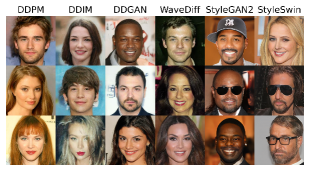
Figure 4: Figure depicting the sample set of images utilized in the user study. Images from all models fill the columns. A supplementary figure shows additional images.

[scale=0.85]figures/user_study/user_study [scale=0.875]figures/user_study/fid [scale=0.85]figures/user_study/dssim [scale=0.85]figures/user_study/wpskl

Figure 5: Comparison of the results of the user study with fid, SSIM, and wpskl. For all plots, lower is better. (a) plots the percentage of pairs where users preferred the real image over the generated image, (b) plots fid, (c) plots the inverse of structural similarity measured as $\frac{1-\text{SSIM}}{2}$, and finally (d) plots our proposed metric score.

We surveyed users to ensure our metrics align with human perception. To this end, we devised a questionnaire with image pairs. The design follows [38]. Users were asked to answer fifty-two questions. For every question, a model-generated image was presented alongside an image from the CelebAHQ dataset. The questionnaire instructed users to choose the real image [38]. Figure 4 depicts a subset of the generated images. Overall, 41 users took part in the study.

Figure 5 presents the results. For every model, a bar indicates the percentage of cases where users chose an original image instead of a synthetic sample from the model. Over half of the users found ddgan and ddpm images convincing. Only a quarter chose ddim images instead of the CelebAHQ-originals. WaveDiff and StyleGAN2 received similar ratings. Overall, especially at the top and bottom of the scale, user ratings are consistent with our proposed metric. As in the user study, wpskl ranks ddgan first. Similarly, users and wpskl rank ddim last. The picture is more nuanced for ddpm. wpskl ranks WaveDiff, StyleGAN2 and StyleSwin similarly and ddpm slightly lower. However, in the user study ddpm is ahead of WaveDiff, StyleGAN2 and StyleSwin. fid is inverse to the user preferences. While DDGAN generates the most realistic images according to the user study, the fid score is higher than for WaveDiff and StyleSwin. Previous works found that ssim scores are unpredictable for human perception [37]. The plot supports this observation since the best (ddpm) and worst (ddim) performing methods in the user study get similar ssim scores.

5.3 Ablation study

The power spectrum can not only be computed for wavelets, but also for Fourier coefficients. In this way, the spatial information is discarded and only the frequency information is considered. For a comparison, we transform the input images using a two-dimensional fft. After normalizing in a manner analogous to Equation (2), we compute the fpskl. The computation resembles Equation (3), but we employ the Fourier transform instead of the wavelet packet transform.

In Table 2, we compare fpskl and wpskl using the CelebAHQ dataset. While $D_{\mathcal{F}}$ ranks as $D_{\mathcal{W}}$ ddgan first, $D_{\mathcal{F}}$ ranks ddpm last whereas $D_{\mathcal{W}}$ ranks ddim last. Considering that ddim performed worst in the user study, this shows that using only frequency information is insufficient and that the wavelet representation provides a better metric.

Given the wavelet representation, we can also investigate model differences with respect to frequencies. To this end, we average over both packet height and width, and thus remove all spatial information. Consequently, we gain insights into the frequency properties of our models. Figure 6 plots mean absolute log scaled wavelet coefficients for images from the CelebAHQ dataset and images generated by ddpm[10] and StyleGAN2 [16]. We see the StyleGAN2 coefficients come closer to the true CelebAHQ spectrum, which explains the lower $\mathcal{D_{F}}$ score for StyleGAN2 in Table 2 on CelebAHQ. Furthermore, we see that the differences increase when we move toward higher frequency packets on the left.

Dataset	Method	$D_{\mathcal{F}}$	$D_{\mathcal{W}}$
CelebAHQ	DDPM [10]	1.35	1.37
	DDIM [40]	1.29	1.59
	WaveDiff [33]	1.27	1.35
	DDGAN [49]	1.27	1.33
	StyleSwin [52]	1.28	1.35
	StyleGAN2 [15]	1.29	1.35

Table 2: Comparing fpskl with wpskl.

[width=.8]./figures/ablation_plots/ln_packetplot_celebAHQ_DDPM_stylegan2_sym5

Figure 6: Mean absolute log scaled wavelet coefficients for DDPM and StyleGAN2 on the CelebAHQ dataset. We averaged the coefficients for each filter. In this way, we remove all spatial information and gain insight into the frequency properties of the methods.

[width=1.0]./figures/ablation_plots/diff_packetimage_haar

Figure 7: Absolute packet difference of the mean ddpm and CelebAHQ packets. After averaging along the channel dimension, we concatenate the 256 filtered images to create a single image. The plot shows the difference of the log scaled absolute wpt coefficients for the original CelebAHQ dataset and ddpm. The packets are in frequency order. The exclusively lowpass-filtered aaaa packet sits on the top left. The frequency increases along the diagonal from the top left to the bottom right. We see significant differences in the higher frequency section of the plot.

The wavelet packet transform, however, not only provides frequency information, but it also conserves spatial information to some degree. We can thus investigate spatial differences as well by looking at the wavelet packet coefficient distribution in detail. For this study, we compute the mean packets using 30 thousand images from CelebAHQ and the same amount of images generated by ddpm. To understand the origin of distribution differences, we plot the difference of the log-scaled mean packet coefficients. Figure 7 shows the coefficient differences for all 256 level four packets. The packets are arranged such that the frequency increases along the diagonal. We see the biggest differences in the fourth quadrant, where the high-frequency packets are. While faces are visible, the surrounding background pixels appear brighter. Figure 7 suggests that ddpm struggles to model high-frequency background patterns correctly. While Figure 6 already suggested problems at higher frequencies, Figure 7 shows that high-frequency errors are often in the background. This is also visible in the few examples shown Figure 4 where the background is rather smooth.

[width=0.8]./python/tikz/noise_normal

Figure 8: fid values are said to be unstable and difficult to reproduce [1]. We compare fid to Fourier and wavelet packet KL-divergence. While $\mathcal{D_{F}}$ and $\mathcal{D_{W}}$ monotonically increase, fid shows large fluctuations. All plots show mean results computed for the first five CelebAHQ images. The shaded areas mark the standard deviation.

Finally, we study the effects of adding Gaussian noise or rotating images on the metrics fid, fpskl, and wpskl. For this study, we use the first five CelebAHQ [13] images. Figure 8 plots the response of fid, fpskl, and wpskl to Gaussian noise disturbances. The plot shows that fid is unstable and that there are large fluctuations as the noise is increased. Such a behavior is undesirable and makes it difficult to reproduce results. fpskl and wpskl increase monotonically as it should be the case.

Figure 9 shows the effect that image rotation has on fid, wpskl and fpskl. We observe that wpskl produces a stable error for rotated images. fid behaves similarly but shows larger fluctuations. The Fourier-based metric fpskl, however, does not capture 180-degree rotations, which also demonstrates that wavelets are a better representation for a metric.

[width=0.8]./python/tikz/rotate

Figure 9: This plot shows the effect of rotation followed by center-cropping to avoid padding. $\mathcal{D_{F}}$ does not differentiate between rotations by 180 degrees. All plots show mean results computed for the first five CelebAHQ images. The shaded areas mark the standard deviation.

5.4 Frequency band guidance

Method	$D_{\mathcal{W}}$
DDPM [10]	1.66
DDIM [40]	1.74
Imp. Diff. (Hybrid) [29]	1.69
Imp. Diff. (VLB) [29]	1.73
WaveDiff [33]	1.68
DDGAN [49]	1.68
StyleGAN2 [15]	1.69
DDPM-WPDL (ours)	1.50

Table 3: Comparison of the DDPM model finetuned with the wavelet-power divergence loss with other approaches on the CIFAR10 dataset.

In Section 4, we introduced an additional wavelet-power divergence loss that can be used to train generative models. To understand its effects, we took a pre-trained ddpm model and finetuned it using only the wavelet guidance loss from Equation (7) for 100 epochs with a learning rate of $1e-5$. Table 3 shows that it significantly reduces the $D_{\mathcal{W}}$ score, in comparison to the original ddpm model and related architectures. Training from scratch with a wavelet-packet loss yielded similar results.

6 Conclusion

Modern generative models are biased towards low-frequency content [5]. Addressing the problem requires metrics, which take frequency information into account. Furthermore, existing pixel-based metrics like ssim are said to be unreliable predictors of human perception [37]. Our user study confirms this. However, we also found that fid was valid only on datasets resembling ImageNet classes. On CelebAHQ’s faces, fid did not reflect user preferences well. Consequently, this paper proposed a new metric for comparing approaches for image synthesis, which jointly considers spatial and frequency information without introducing an ImageNet bias. The proposed metric generally agrees with users’ verdict on the CelebAHQ dataset. While the metric has major advantages compared to fid, it is not a metric of human perception and it can be combined with other metrics.

Acknowledgements Research was supported by the Bundesministerium für Bildung und Forschung (BMBF) via the WestAI and BnTrAInee projects. The authors gratefully acknowledge the Gauss Centre for Supercomputing e.V. (www.gauss-centre.eu) for funding this project by providing computing time through the John von Neumann Institute for Computing (NIC) on the GCS Supercomputer JUWELS at Jülich Supercomputing Centre (JSC).

 

7 Supplementary

7.1 The fast wavelet and wavelet packet transforms

This supplementary section summarizes key wavelet facts as a convenience for the reader. See, for example, [41, 25] or [12] for excellent detailed introductions to the topic.

The fwt relies on convolution operations with filter pairs.

[scale=0.9]./figures/supplementary/fwt

Figure 10: Overview of the fwt computation. $\mathbf{h}_{\mathcal{L}}$ denotes the analysis low-pass filter and $\mathbf{h}_{\mathcal{H}}$ the analysis high pass filter. $\mathbf{f}_{\mathcal{L}}$ and $\mathbf{f}_{\mathcal{H}}$ the synthesis filter pair. $\downarrow_{2}$ denotes downsampling with a factor of two, $\uparrow_{2}$ means upsampling. The analysis transform relies on stride two convolutions. The synthesis or inverse transform on the right works with stride two transposed convolutions. $\mathbf{H}_{k}$ and $\mathbf{F}_{k}$ with $k\in[\mathcal{L},\mathcal{H}]$ denote the corresponding convolution operators.

Figure 10 illustrates the process. The forward or analysis transform works with a low-pass $\mathbf{h}_{\mathcal{L}}$ and a high-pass filter $\mathbf{h}_{\mathcal{H}}$. The analysis transform repeatedly convolves with both filters,

$$\mathbf{x}_{s}*\mathbf{h}_{k}=\mathbf{c}_{k,s+1}$$ (8)

with $k\in[\mathcal{L},\mathcal{H}]$ and $s\in\mathbb{N}_{0}$ the set of natural numbers, where $\mathbf{x}_{0}$ is equal to the original input signal $\mathbf{x}$. At higher scales, the fwt uses the low-pass filtered result as input, $\mathbf{x}_{s}=\mathbf{c}_{\mathcal{L},s}$ if $s>0$. The dashed arrow in Figure 10 indicates that we could continue to expand the fwt tree here.

The wpt additionally expands the high-frequency part of the tree.

[scale=0.9]./figures/supplementary/packets_1d

Figure 11: Scematic drawing of the full wpt in a single dimension. Compared to Figure 10, the high-pass filtered side of the tree is expanded, too.

A comparison of Figures 10 and 11 illustrates this difference. Whole expansion is not the only possible way to construct a wavelet packet tree. See [12] for a discussion of other options. In both figures, capital letters denote convolution operators. These may be expressed as Toeplitz matrices [41]. The matrix nature of these operators explains the capital boldface notation. Coefficient subscripts record the path that leads to a particular coefficient.

We construct filter quadruples from the original filter pairs to process two-dimensional inputs. The process uses outer products [44]:

$$\mathbf{h}_{a}=\mathbf{h}_{\mathcal{L}}\mathbf{h}_{\mathcal{L}}^{T},\mathbf{h}_{h}=\mathbf{h}_{\mathcal{L}}\mathbf{h}_{\mathcal{H}}^{T},\mathbf{h}_{v}=\mathbf{h}_{\mathcal{H}}\mathbf{h}_{\mathcal{L}}^{T},\mathbf{h}_{d}=\mathbf{h}_{\mathcal{H}}\mathbf{h}_{\mathcal{H}}^{T}$$ (9)

With $a$ for approximation, $h$ for horizontal, $v$ for vertical, and $d$ for diagonal [19]. We can construct a wpt-tree for images with these two-dimensional filters.

[scale=0.9]./figures/supplementary/packets_2d

Figure 12: Two dimensional wpt computation overview. $\mathbf{X}$ and $\hat{\mathbf{X}}$ denote input image and reconstruction respectively. We compute wpskl using the wavelet packet coefficients $\mathbf{p}$.

Figure 12 illustrates the computation of a full two-dimensional wavelet packet tree. More formally, the process initially evaluates

$$\mathbf{x}_{0}*_{2}\mathbf{h}_{j}=\mathbf{c}_{j,1}$$ (10)

with $\mathbf{x}_{0}$ equal to an input image $\mathbf{X}$, $j\in[a,h,v,d]$, and $*_{2}$ for two-dimensional convolution. At higher scales, all resulting coefficients from previous scales serve as inputs. The four filters are repeatedly convolved with all outputs to build the full tree. The inverse transforms work analogously. We refer to the standard literature [12, 41] for an extended discussion.

Compared to the fwt, the high-frequency half of the tree is subdivided into more bins, yielding a fine-grained view of the entire spectrum. We always show analysis and synthesis transforms to stress that all wavelet transforms are lossless. Synthesis transforms reconstruct the original input based on the results from the analysis transform.

7.2 Common wavelets and their properties

A key property of the wavelet transform is its invertibility. Additionally, we expect an alias-free representation. Standard literature like [41] formulates the perfect reconstruction and alias cancellation conditions to satisfy both requirements. For an analysis filter coefficient vector $\mathbf{h}$, the equations below use the polynomial $H(z)=\sum_{n}h(n)z^{-n}$. We construct $F(z)$ the same way using the synthesis filter coefficients in $\mathbf{f}$. To guarantee perfect reconstruction the filters must respect

$$H_{\mathcal{L}}(z)F_{\mathcal{L}}(z)+H_{\mathcal{H}}(-z)F_{\mathcal{H}}(z)=2z^{-l}.$$ (11)

Similarly

$$F_{\mathcal{L}}(z)H_{\mathcal{L}}(-z)+F_{\mathcal{H}}(z)H_{\mathcal{H}}(-z)=0$$ (12)

guarantees alias cancellation.

Filters that satisfy both equations qualify as wavelets. Examples are Daubechies wavelets and Symlets.

./figures/supplementary/sym6

Figure 13: Visualization of the Symlet 6 filter coefficients.

./figures/supplementary/db6

Figure 14: Visualization of the Daubechies 6 filter coefficients.

Figures 13 and 14 visualize the Daubechies and Symlet filters of 6th degree. Compared to the Daubechies wavelet family, their Symlet cousins have more mass at the center. Figure 13 illustrates this fact. Large deviations occur around the fifth filter in the center, unlike the Daubechies’ six filters in Figure 14. Consider the sign patterns in Figure 14. The decomposition highpass (orange) and the reconstruction lowpass (green) filters display an alternating sign pattern. This behavior is a possible solution to the alias cancellation condition, which can be seen by substituting $F_{\mathcal{L}}(z)=H_{\mathcal{H}}(-z)$ and $F_{\mathcal{H}}=-H_{\mathcal{L}}(-z)$ into Equation (12) [41]. $F_{\mathcal{L}}(z)=H_{\mathcal{H}}(-z)$ requires an opposing sign at even and equal signs at odd powers of the polynomial.

Using the wavelet filter as described above, we can compute a wavelet packet transform as described in section 7.1. We denote the wavelet packet transform as $\mathcal{W}_{p}$. It appears in equation 2 in the main text.

7.3 fid sensitivity and reproduction problems

Figures 8 and 9 provide an analysis of the sensitivity of fid concerning a variety of input perturbations, specifically Gaussian noise and rotation. In Figure 15, we investigate one more input perturbation, namely Gaussian blur. In this setup, Gaussian blur is applied with a growing blur intensity. The results reveal that all three metrics react proportionally, with our metric wpskl having a smaller standard deviation. Gaussian blur attenuates frequencies in the image in proportion to blur intensity. This results in a higher standard deviation.

[width=0.6]./python/tikz/blur

Figure 15: Effect of Gaussian blur on all the three metrics FID, wpskl and fpskl. All three metrics react proportionally to increasing the Gaussian blur intensity.

7.4 Additional Wavelet Packet Plots

In Figure 7, we introduced a plot depicting the absolute mean packet difference between DDPM and CelebAHQ dataset packets. In Figure 16, we depict the individual log-scaled absolute wavelet mean packets for both the CelebAHQ dataset and DDPM-generated images. We compute a level four decomposition on both sets of images with sym5 wavelets. In accordance with Figure 7, comparing Figures 7 and 16 shows that the DDPM packets are more noisy than the packets of the original dataset, especially in the fourth quadrant.

(a) CelebAHQ packets

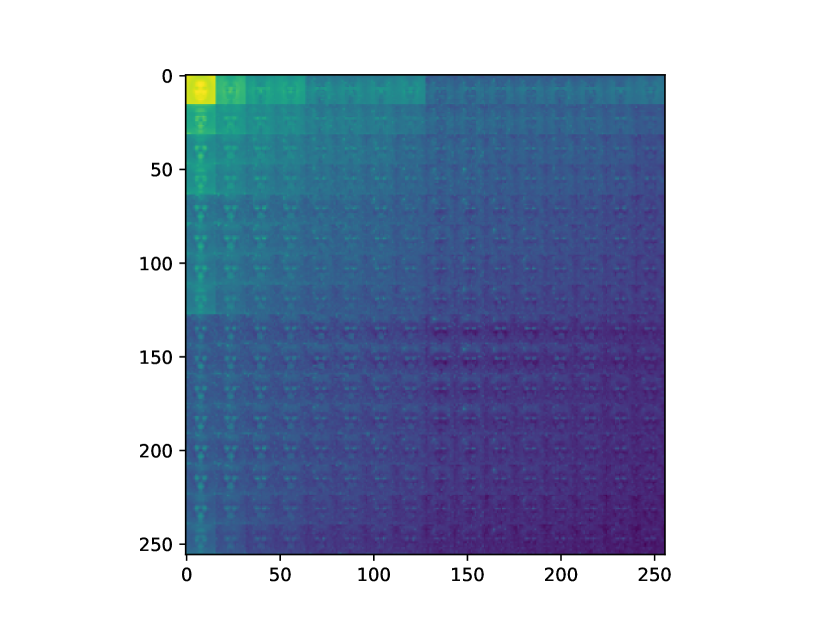
(b) DDPM packets

Figure 16: Mean packet representation for CelebAHQ dataset in (a) and DDPM generated images in (b). Packets are computed using sym5 wavelet with wavelet decomposition level of 4, resulting in 256 packets.

In addition to packets, we explore the effect of choice of wavelet on our metric wpskl, as depicted in Figure 17. The class of Daubechies wavelets extends the Haar wavelet. Consequently, the Haar wavelet is also the Daubechies-1 wavelet. As the Daubechies wavelet degree increases, we observe a reduction in wpskl value. Conversely, with symlets, we notice only a minor reduction in wpskl value. This experiment utilizes the first 10000 images of CelebAHQ and DDPM-generated images. This smaller rate of change of the symlet-wpskl with increasing wavelet degree motivates our selection of symlet for evaluation of wpskl. The choice of the degree is less important, but we always use a symlet with degree of 5.

[width=0.95]./figures/supplementary/wpskl_v_wavelets

Figure 17: Effect of wavelet choice on wpskl. wpskl depict a decreasing trend with Daubechies wavelet represented in red points. Where as Symlets represented in blue also show a decreasing trend but with a minor rate of change. Haar wavelet can be viewed as analogous to Daubechies-1 wavelet. wpskl is calculated with DDPM-CelebAHQ images.

7.5 User Study

Figure 18 depicts an additional set of images from each model. The predominant consensus among users in the user study indicates that they largely relied on the background of the images as a critical feature in discriminating realistic images. This is further corroborated by Figure 7, wherein higher energy is visible in the background. Other than background, subtle differences like eye colours (notably in StyleSwin) and hair texture contribute to finding realistic images. Few StyleGAN2 images depict strong artifacts, e.g., the first StyleGAN2 image in Figure 18.

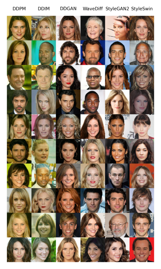
Figure 18: An additional set of images from the user study.

References

- [1] Evaluating diffusion models. https://huggingface.co/docs/diffusers/conceptual/evaluation, 2023. Accessed: 2023-10-24.
- [2] Martin Arjovsky, Soumith Chintala, and Léon Bottou. Wasserstein generative adversarial networks. In International conference on machine learning, pages 214–223. PMLR, 2017.
- [3] Min Jin Chong and David A. Forsyth. Effectively unbiased FID and inception score and where to find them. In 2020 IEEE/CVF Conference on Computer Vision and Pattern Recognition, CVPR 2020, Seattle, WA, USA, June 13-19, 2020, pages 6069–6078. Computer Vision Foundation / IEEE, 2020.
- [4] Ingrid Daubechies. Ten Lectures on Wavelets. Society for Industrial and Applied Mathematics, 1992.
- [5] Ricard Durall, Margret Keuper, and Janis Keuper. Watch your up-convolution: Cnn based generative deep neural networks are failing to reproduce spectral distributions. In Proceedings of the IEEE/CVF conference on computer vision and pattern recognition, pages 7890–7899, 2020.
- [6] Rinon Gal, Dana Cohen Hochberg, Amit Bermano, and Daniel Cohen-Or. Swagan: A style-based wavelet-driven generative model. ACM Trans. Graph., 40(4), July 2021.
- [7] Florentin Guth, Simon Coste, Valentin De Bortoli, and Stephane Mallat. Wavelet score-based generative modeling. Advances in Neural Information Processing Systems, 35:478–491, 2022.
- [8] Alejandro Hernandez, Jurgen Gall, and Francesc Moreno-Noguer. Human motion prediction via spatio-temporal inpainting. In Proceedings of the IEEE/CVF International Conference on Computer Vision, pages 7134–7143, 2019.
- [9] Martin Heusel, Hubert Ramsauer, Thomas Unterthiner, Bernhard Nessler, and Sepp Hochreiter. Gans trained by a two time-scale update rule converge to a local nash equilibrium. Advances in neural information processing systems, 30, 2017.
- [10] Jonathan Ho, Ajay Jain, and Pieter Abbeel. Denoising diffusion probabilistic models. In Hugo Larochelle, Marc’Aurelio Ranzato, Raia Hadsell, Maria-Florina Balcan, and Hsuan-Tien Lin, editors, Advances in Neural Information Processing Systems 33: Annual Conference on Neural Information Processing Systems 2020, NeurIPS 2020, December 6-12, 2020, virtual, 2020.
- [11] Huaibo Huang, Ran He, Zhenan Sun, and Tieniu Tan. Wavelet-srnet: A wavelet-based cnn for multi-scale face super resolution. In Proceedings of the IEEE international conference on computer vision, pages 1689–1697, 2017.
- [12] Arne Jensen and Anders la Cour-Harbo. Ripples in mathematics: the discrete wavelet transform. Springer Science & Business Media, 2001.
- [13] Tero Karras, Timo Aila, Samuli Laine, and Jaakko Lehtinen. Progressive growing of gans for improved quality, stability, and variation. In 6th International Conference on Learning Representations, ICLR 2018, Vancouver, BC, Canada, April 30 - May 3, 2018, Conference Track Proceedings, 2018.
- [14] Tero Karras, Miika Aittala, Samuli Laine, Erik Härkönen, Janne Hellsten, Jaakko Lehtinen, and Timo Aila. Alias-free generative adversarial networks. Advances in Neural Information Processing Systems, 34:852–863, 2021.
- [15] Tero Karras, Samuli Laine, and Timo Aila. A style-based generator architecture for generative adversarial networks. In Proceedings of the IEEE/CVF conference on computer vision and pattern recognition, pages 4401–4410, 2019.
- [16] Tero Karras, Samuli Laine, Miika Aittala, Janne Hellsten, Jaakko Lehtinen, and Timo Aila. Analyzing and improving the image quality of stylegan. In Proceedings of the IEEE/CVF conference on computer vision and pattern recognition, pages 8110–8119, 2020.
- [17] Alex Krizhevsky, Geoffrey Hinton, et al. Learning multiple layers of features from tiny images. 2009.
- [18] Tuomas Kynkäänniemi, Tero Karras, Miika Aittala, Timo Aila, and Jaakko Lehtinen. The role of imagenet classes in fréchet inception distance. In The Eleventh International Conference on Learning Representations, ICLR 2023, Kigali, Rwanda, May 1-5, 2023. OpenReview.net, 2023.
- [19] Gregory Lee, Ralf Gommers, Filip Waselewski, Kai Wohlfahrt, and Aaron O’Leary. Pywavelets: A python package for wavelet analysis. Journal of Open Source Software, 4(36):1237, 2019.
- [20] Jin Li, Wanyun Li, Zichen Xu, Yuhao Wang, and Qiegen Liu. Wavelet transform-assisted adaptive generative modeling for colorization. IEEE Transactions on Multimedia, 2022.
- [21] Lin Liu, Jianzhuang Liu, Shanxin Yuan, Gregory Slabaugh, Aleš Leonardis, Wengang Zhou, and Qi Tian. Wavelet-based dual-branch network for image demoiréing. In Computer Vision–ECCV 2020: 16th European Conference, Glasgow, UK, August 23–28, 2020, Proceedings, Part XIII 16, pages 86–102. Springer, 2020.
- [22] Yunfan Liu, Qi Li, and Zhenan Sun. Attribute-aware face aging with wavelet-based generative adversarial networks. In Proceedings of the IEEE/CVF Conference on Computer Vision and Pattern Recognition, pages 11877–11886, 2019.
- [23] Lorenzo Luzi, Carlos Ortiz Marrero, Nile Wynar, Richard G. Baraniuk, and Michael J. Henry. Evaluating generative networks using gaussian mixtures of image features. In IEEE/CVF Winter Conference on Applications of Computer Vision, WACV 2023, Waikoloa, HI, USA, January 2-7, 2023, pages 279–288. IEEE, 2023.
- [24] Stéphane Mallat. A theory for multiresolution signal decomposition: The wavelet representation. IEEE Trans. Pattern Anal. Mach. Intell., 11(7):674–693, 1989.
- [25] Stéphane Mallat. A wavelet tour of signal processing. Elsevier, 1999.
- [26] Moritz Wolter. Frequency Domain Methods in Recurrent Neural Networks for Sequential Data Processing. PhD thesis, Rheinische Friedrich-Wilhelms-Universität Bonn, July 2021.
- [27] Muhammad Ferjad Naeem, Seong Joon Oh, Youngjung Uh, Yunjey Choi, and Jaejun Yoo. Reliable fidelity and diversity metrics for generative models. In International Conference on Machine Learning, pages 7176–7185. PMLR, 2020.
- [28] Apollo 11 NASA. Ocean world earth. https://commons.wikimedia.org/wiki/File:Ocean_world_Earth.jpg, 1969. Accessed: 2023-10-31.
- [29] Alexander Quinn Nichol and Prafulla Dhariwal. Improved denoising diffusion probabilistic models. In Proceedings of the 38th International Conference on Machine Learning, volume 139 of Proceedings of Machine Learning Research, pages 8162–8171. PMLR, 18–24 Jul 2021.
- [30] Gaurav Parmar, Richard Zhang, and Jun-Yan Zhu. On aliased resizing and surprising subtleties in gan evaluation. In Proceedings of the IEEE/CVF Conference on Computer Vision and Pattern Recognition, pages 11410–11420, 2022.
- [31] Adam Paszke, Sam Gross, Soumith Chintala, Gregory Chanan, Edward Yang, Zachary DeVito, Zeming Lin, Alban Desmaison, Luca Antiga, and Adam Lerer. Automatic differentiation in pytorch. In 31st Conference on Neural Information Processing Systems (NIPS 2017), 2017.
- [32] William Peebles and Saining Xie. Scalable diffusion models with transformers. arXiv preprint arXiv:2212.09748, 2022.
- [33] Hao Phung, Quan Dao, and Anh Tran. Wavelet diffusion models are fast and scalable image generators. In IEEE/CVF Conference on Computer Vision and Pattern Recognition, CVPR 2023, Vancouver, BC, Canada, June 17-24, 2023, pages 10199–10208. IEEE, 2023.
- [34] Photoplay Publishing. Albert einstein and charlie chaplin city lights premiere 1931. https://commons.wikimedia.org/wiki/File:Albert_Einstein_and_Charlie_Chaplin_City_Lights_premiere_1931.jpg, 1931. Accessed: 2023-11-09.
- [35] Nasim Rahaman, Aristide Baratin, Devansh Arpit, Felix Draxler, Min Lin, Fred Hamprecht, Yoshua Bengio, and Aaron Courville. On the spectral bias of neural networks. In International Conference on Machine Learning, pages 5301–5310. PMLR, 2019.
- [36] Olga Russakovsky, Jia Deng, Hao Su, Jonathan Krause, Sanjeev Satheesh, Sean Ma, Zhiheng Huang, Andrej Karpathy, Aditya Khosla, Michael Bernstein, Alexander C. Berg, and Li Fei-Fei. ImageNet Large Scale Visual Recognition Challenge. International Journal of Computer Vision (IJCV), 115(3):211–252, 2015.
- [37] Chitwan Saharia, William Chan, Huiwen Chang, Chris Lee, Jonathan Ho, Tim Salimans, David Fleet, and Mohammad Norouzi. Palette: Image-to-image diffusion models. In ACM SIGGRAPH 2022 Conference Proceedings, pages 1–10, 2022.
- [38] Tim Salimans, Ian Goodfellow, Wojciech Zaremba, Vicki Cheung, Alec Radford, and Xi Chen. Improved techniques for training gans. Advances in neural information processing systems, 29, 2016.
- [39] Vishwanath Saragadam, Daniel LeJeune, Jasper Tan, Guha Balakrishnan, Ashok Veeraraghavan, and Richard G Baraniuk. Wire: Wavelet implicit neural representations. In Proceedings of the IEEE/CVF Conference on Computer Vision and Pattern Recognition, pages 18507–18516, 2023.
- [40] Jiaming Song, Chenlin Meng, and Stefano Ermon. Denoising diffusion implicit models. In 9th International Conference on Learning Representations, ICLR 2021, Virtual Event, Austria, May 3-7, 2021, 2021.
- [41] Gilbert Strang and Truong Nguyen. Wavelets and filter banks. SIAM, 1996.
- [42] Christian Szegedy, Vincent Vanhoucke, Sergey Ioffe, Jon Shlens, and Zbigniew Wojna. Rethinking the inception architecture for computer vision. In Proceedings of the IEEE conference on computer vision and pattern recognition, pages 2818–2826, 2016.
- [43] Stéfan van der Walt, Johannes L. Schönberger, Juan Nunez-Iglesias, François Boulogne, Joshua D. Warner, Neil Yager, Emmanuelle Gouillart, Tony Yu, and the scikit-image contributors. scikit-image: image processing in Python. PeerJ, 2:e453, 6 2014.
- [44] Aparna Vyas, Soohwan Yu, and Joonki Paik. Multiscale transforms with application to image processing. Springer, 2018.
- [45] Jianyi Wang, Xin Deng, Mai Xu, Congyong Chen, and Yuhang Song. Multi-level wavelet-based generative adversarial network for perceptual quality enhancement of compressed video. In European Conference on Computer Vision, pages 405–421. Springer, 2020.
- [46] Zhou Wang, Alan C Bovik, Hamid R Sheikh, and Eero P Simoncelli. Image quality assessment: from error visibility to structural similarity. IEEE transactions on image processing, 13(4):600–612, 2004.
- [47] Travis Williams and Robert Li. Wavelet pooling for convolutional neural networks. In International conference on learning representations, 2018.
- [48] Moritz Wolter, Felix Blanke, Raoul Heese, and Jochen Garcke. Wavelet-packets for deepfake image analysis and detection. Machine Learning, 111(11):4295–4327, 2022.
- [49] Zhisheng Xiao, Karsten Kreis, and Arash Vahdat. Tackling the generative learning trilemma with denoising diffusion gans. In International Conference on Learning Representations, 2022.
- [50] Jaejun Yoo, Youngjung Uh, Sanghyuk Chun, Byeongkyu Kang, and Jung-Woo Ha. Photorealistic style transfer via wavelet transforms. In Proceedings of the IEEE/CVF International Conference on Computer Vision, pages 9036–9045, 2019.
- [51] Fisher Yu, Yinda Zhang, Shuran Song, Ari Seff, and Jianxiong Xiao. Lsun: Construction of a large-scale image dataset using deep learning with humans in the loop. ArXiv, abs/1506.03365, 2015.
- [52] Bowen Zhang, Shuyang Gu, Bo Zhang, Jianmin Bao, Dong Chen, Fang Wen, Yong Wang, and Baining Guo. Styleswin: Transformer-based gan for high-resolution image generation. In Proceedings of the IEEE/CVF conference on computer vision and pattern recognition, pages 11304–11314, 2022.