Understanding Normalization in Contrastive Representation Learning and Out-of-Distribution Detection

Abstract

Contrastive representation learning has emerged as an outstanding approach for anomaly detection. In this work, we explore the $\ell_{2}$-norm of contrastive features and its applications in out-of-distribution detection. We propose a simple method based on contrastive learning, which incorporates out-of-distribution data by discriminating against normal samples in the contrastive layer space. Our approach can be applied flexibly as an outlier exposure (OE) approach, where the out-of-distribution data is a huge collective of random images, or as a fully self-supervised learning approach, where the out-of-distribution data is self-generated by applying distribution-shifting transformations. The ability to incorporate additional out-of-distribution samples enables a feasible solution for datasets where AD methods based on contrastive learning generally underperform, such as aerial images or microscopy images. Furthermore, the high-quality features learned through contrastive learning consistently enhance performance in OE scenarios, even when the available out-of-distribution dataset is not diverse enough. Our extensive experiments demonstrate the superiority of our proposed method under various scenarios, including unimodal and multimodal settings, with various image datasets.

1 Introduction

Out-of-distribution (OOD) detection, or anomaly detection (AD), is the task of distinguishing between normal and out-of-distribution (abnormal) data, with the general assumption that access to abnormal data is prohibited. Therefore, OOD detection methods [12]; [16]; [36] are typically carried out in an unsupervised manner where only normal data is available. In this regard, approaches based on self-supervised learning or pre-trained models, which are capable of extracting deep features without explicitly requiring labeled data, are commonly utilized to solve OOD detection problems.

However, the presumption that access to non-nominal data is forbidden is not highly restricted. Especially in image OOD detection problems, one can gather randomly natural image datasets that are likely not-normal on the internet. The utilization of such data is called Outlier Exposure [15]. Several top-performing AD methods, including unsupervised [25], self-supervised [16], and pre-trained [29]; [9] approaches, utilize tens of thousands of OE samples to enhance their performance and achieve state-of-the-art detection accuracy. Nevertheless, it is important to note that Outlier Exposure (OE) also has its limitations, especially when the anomalies are subtle or when the normal data is highly diverse [25].

One of the most effective OOD detection techniques, CSI [36] is constructed by combining a special form of contrastive learning, SimCLR [6], with a geometric OOD detection approach [16]. SimCLR encourages augmented views of a sample to attract each other while repelling them to a negative corpus consisting of views of other samples. CSI suggests that the addition of sufficiently distorted augmentations to the negative corpus improves OOD detection performance. Simultaneously, the network has to classify each sample’s type of transformation, as in [16]. For a test sample, the anomaly score is determined by both the trained network’s confidence in correctly predicting the sample’s transformations and the sample’s similarity to its nearest neighbor in the feature space. However, similar to geometric approaches [16]; [12], CSI performance depends on the relationship between normal data and shifted transformations (e.g., symmetry images and rotations).

Inspired by the strengths and weaknesses of both approaches, we propose Outlier Exposure framework for Contrastive Learning (OECL), an OE extension for contrastive learning OOD detection methods. By manipulating $\ell_{2}$-norm of samples on the contrastive space, we found a simple way to integrate OOD samples into SimCLR-based methods. The high quality deep representations obtained by contrastive learning and the“anomalousness” from OOD samples allow our approach to address the limitations of the both original approaches. To validate our claims, we conducted extensive experiments in various environments, including the common unimodal setting, the newly challenging multimodal setting and our newly introduced few-shot OOD setting. Our main contributions are summarized as follows:

1. We propose a simple yet effective method, OECL, to incorporate out-of-distribution data to contrastive learning AD methods. The out-of-distribution data can be chosen from an external out-of-distribution dataset or self-generated by sufficiently distorted transformations.

2. We provide insight into the $\ell_{2}$-normalization in contrastive learning and its application in OOD detection.

2 Related work

OOD detection. A growing area of research uses self-supervision for OOD detection. They train a network with a pre-defined task on the training set and utilize the rich features to improve OOD detection performances. These approaches have demonstrated remarkable performance in OOD detection, pushing the boundaries of what is achievable in this field [36]; [12]; [16]; [39]; [35].

More recently, transfer learning-based methods have revolutionized OOD detection [25]; [29]; [8]; [27]; [4]; [9]. These approaches involve fine-tuning supervised classifiers that were originally trained on large datasets [28]. This fine-tuning process adapts these classifiers to OOD detection tasks and has been shown to outperform the self-supervised methods on common benchmarks. Importantly, transfer learning-based approaches have provided powerful tools for research in defect detection.

Another research field in OOD detection is about incorporating outliers to improve the performance of unsupervised OOD detection methods [25]; [15]; [32]; [33]; [24]; [20]. For instance, [15] uses OE to improve their self-supervised method by forcing the network to predict the uniform distribution for OE samples. [3] uses OE as a penalty to hinder the student model from generalizing its imitation of the teacher model to out-of-distribution images.

Non-standard image OOD detection. Recently, there has been a growing interest in “non-standard” image OOD detection. Unlike the common CIFAR-10 or ImageNet, these non-standard datasets have unique characteristics that challenge OOD detection methods. One such challenge is presented by datasets where normal and abnormal samples are semantically identical but differ in their local appearances. Datasets with such a characteristic are primarily objects in defect detection research [30]; [3]; [24]. Another category of non-standard datasets arises from the distinctive physical properties of training images, such as rotation-invariant images. In these cases, recent unsupervised methods [36]; [12] have faced limitations as shown in our experiments. Datasets belong to this ’distinctive physical’ category and standard images are our main focus in this paper.

3 Contrastive Learning and Anomaly Detection

Suppose we are given an unlabeled dataset $\mathcal{D}=\left\{x_{i}\right\}_{i=1}^{N}$ sampled from a distribution $p_{\text{data}}(x)$ over $\mathbb{R}^{n}$. The goal of anomaly detection is to construct a detector that identifies whether $x$ is sampled from $p_{\text{data}}$ or not. However, directly modeling an accurate model of $p_{\text{data}}$ is impractical or infeasible in most cases. To address this, many existing approaches to anomaly detection instead rely on defining a scoring function $s(x)$, with a high value indicating that $x$ is likely to belong to the in-distribution.

3.1 Normalization in Contrastive Learning

Contrastive learning framework. Contrastive learning aims to learn an encoder by maximizing agreement between positive pairs. Empirically, given a set of pre-determined transformations $T$, the positive pairs are obtained by applying randomly two transformations to the same sample, e.g., two affine transformations of the same picture $x$ [6]; [14]; [2]. These positive samples are also regarded as a surrogate class of $x$ [11]. In this paper, we investigate the specific and widely popular form of contrastive loss where the training encoder $z(x)\triangleq f(x)/\lVert f(x)\rVert:\mathbb{R}^{n}\to\mathcal{S}^{m-1}$ maps data to a hypersphere of dimension $m-1$. This loss has been outstandingly successful in anomaly detection literature [36]; [34]; [43],

$$\mathcal{L}_{\text{contrastive}}(z;\tau,M) \triangleq\underset{\begin{subarray}{c}(x,y)\sim p_{\text{pos}}\\ \left\{x_{i}^{-}\right\}_{i=1}^{M}\overset{\text{i.i.d}}{\sim}p_{\text{data}}\end{subarray}}{\mathbb{E}}\left[-\log\frac{e^{z(x)^{t}z(y)/\tau}}{e^{z(x)^{t}z(y)}+\sum_{i}e^{z(x_{i}^{-})^{t}z(y)/\tau}}\right],$$ (1)

where $\tau$ is a temperature hyperparameter, $M$ is a fixed number of negative samples in a mini-batch and $p_{\text{pos}}$ is the distribution of positive pairs over $\mathbb{R}^{n}\times\mathbb{R}^{n}$. This loss can be decoupled into alignment loss and uniformity loss as in [40]:

$$\mathcal{L}_{\text{align}} =\underset{(x,y)\sim p_{\text{pos}}}{\mathbb{E}}\left[-z(x)^{t}z(y)/\tau\right]$$ (2)

$$\mathcal{L}_{\text{uniform}} =\underset{\begin{subarray}{c}(x,y)\sim p_{\text{pos}}\\ \left\{x_{i}^{-}\right\}_{i=1}^{M}\overset{\text{i.i.d}}{\sim}p_{\text{data}}\end{subarray}}{\mathbb{E}}\left[\log\left(e^{z(x)^{t}z(y)}+\sum_{i}e^{z(x_{i}^{-})^{t}z(y)/\tau}\right)\right]$$ (3)

The first term $\mathcal{L}_{\text{align}}$ encourages samples from the same surrogate class be mapped to nearby features. Meanwhile, $\mathcal{L}_{\text{uniform}}$ maximizes averages distances between all samples, leading to features vectors roughly uniformly distributed on the unit hypersphere $\mathcal{S}^{m-1}$.

3.2 $\ell_{2}$-norm of contrastive features

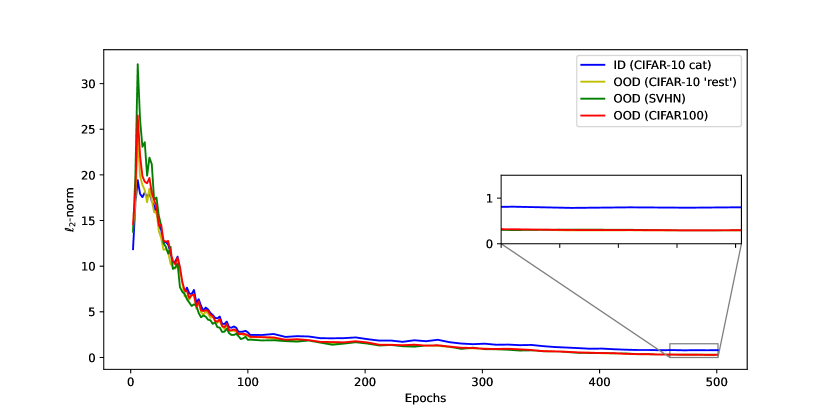
Figure 1: $\ell_{2}$-norm of contrastive features for both normal and OOD samples during optimization of $\mathcal{L}_{\text{contrastive}}$ using only normal samples. Following a few epochs of rapid increase, the $\ell_{2}$-norm for both normal and OOD samples gradually decreases. Notably, as training progresses, the $\ell_{2}$-norm of the training samples becomes larger than that of the OOD samples.

In [36], it was observed that the $\ell_{2}$-norm of contrastive features is effective in detecting anomalies, with normal samples tend to exhibit a larger $\ell_{2}$-norm. CSI [36] suspects that “increasing the norm maybe an easier way to maximize cosine similarity between two vectors: instead of directly reducing the feature distance of two augmented samples, one can also increase the overall norm of the features to reduce the relative distance of two samples”. Our study sheds further light on the behavior of the $\ell_{2}$-norm: contrastive learning gradually reduces the $\ell_{2}$-norm of contrastive features, while the alignment loss compels a significantly larger $\ell_{2}$-norm for the contrastive features of training samples.

Gradual reduction of $\ell_{2}$-norm of contrastive features. This is a phenomenon we observed in many settings using contrastive loss functions based on cosine similarity. As illustrated in fig. 1, following a few epochs of rapid increase, the $\ell_{2}$-norm of both normal and OOD samples gradually decreases. We suspect that this phenomenon is a natural outcome of employing cosine similarity along the interacting between $\mathcal{L}_{\text{align}}$ and $\mathcal{L}_{\text{uniform}}$. We provide further detailed analysis and experiments about this phenomenon in appendix B.

A larger $\ell_{2}$-norm of normal contrastive features. As training progresses, the $\ell_{2}$-norm of the normal samples becomes larger than that of the OOD samples, as shown in fig. 1. To understand this behavior, let’s assume that the surrogate classes $\left\{f(t(x))\right\}_{t\sim T}$ are normally distributed. Since the cosine between two vectors is invariant under rotations, we can assume without loss of generality that $\mathbb{E}_{t\sim T}f(t(x))=\left(\mu,0,\ldots,0\right)$. The following theorem provides a clear illustration of the relationship between contrastive features and alignment in contrastive learning.

[][end, restate] Given two vectors $\bm{X}=\left(X_{1},X_{2},\ldots,X_{n}\right)^{t}$ and $\bm{Y}=\left(Y_{1},Y_{2},\ldots,Y_{n}\right)^{t}$ are i.i.d $\mathcal{N}(\bm{\mu},\bm{\Sigma})$ where $\bm{\mu}=\left(\mu,0,\ldots,0\right)^{t},$ $\mu\geq 0$ and $\bm{\Sigma}=\begin{bmatrix}\sigma&\bm{0}\\ \bm{0}&\Sigma_{V}\end{bmatrix}$. Then,

1. $\mathbb{E}\left\langle\frac{\bm{X}}{\lVert\bm{X}\rVert},\frac{\bm{Y}}{\lVert\bm{Y}\rVert}\right\rangle$ is an increasing function of $\mu$

2. The following inequalities hold

   $$\left(\Phi\left(\frac{\mu}{\sigma}\right)-\Phi\left(-\frac{\mu}{\sigma}\right)\right)^{2} \geq\mathbb{E}\left\langle\frac{\bm{X}}{\lVert\bm{X}\rVert},\frac{\bm{Y}}{\lVert\bm{Y}\rVert}\right\rangle$$ (4)

   $$\mathbb{E}\left\langle\frac{\bm{X}}{\lVert\bm{X}\rVert},\frac{\bm{Y}}{\lVert\bm{Y}\rVert}\right\rangle\geq\frac{1}{1+\frac{\sigma_{V}^{2}}{\epsilon^{2}\mu^{2}}} \left(\Phi\left(\frac{(1-\epsilon)\mu}{\sigma}\right)-\Phi\left(\frac{-(1+\epsilon)\mu}{\sigma}\right)\right)^{2}~{}\forall\epsilon>0,$$ (5)

   where $\sigma_{V}^{2}=\text{tr}\left(\Sigma_{V}\right)$ and $\Phi$ is the cumulative distribution function of $\mathcal{N}(0,1)$.

Since $EX_{i}=0$ for $i\geq 2$ and they are jointly normal distribution, we have

$$\mathbb{E}\frac{X_{i}}{\sqrt{X_{1}^{2}+X_{2}^{2}+\ldots+X_{n}^{2}}}=0~{}\forall i\in\left\{2,\dots,n\right\}.$$

Hence,

$$\mathbb{E}\left\langle\frac{\bm{X}}{\lVert\bm{X}\rVert},\frac{\bm{Y}}{\lVert\bm{Y}\rVert}\right\rangle =\mathbb{E}\frac{X_{1}Y_{1}}{\lVert\bm{X}\rVert\lVert\bm{Y}\rVert}+\sum_{i=2}^{n}\mathbb{E}\frac{X_{i}Y_{i}}{\lVert\bm{X}\rVert\lVert\bm{Y}\rVert}=\left(\mathbb{E}\left[\frac{X_{1}}{\lVert\bm{X}\rVert}\right]\right)^{2}$$

Let denote $U=X_{1}$, $V=\left(X_{2},\ldots,X_{n}\right)^{t}$ and $Z=\lVert V\rVert_{2}^{2}=\sum_{i=2}^{n}X_{i}^{2}$. The expectation of cosine similarity between two vectors $\bm{X}$ and $\bm{Y}$ becomes

$$\left(\frac{1}{\sigma\sqrt{2\pi}}\int_{-\infty}^{\infty}\frac{u}{\sqrt{u^{2}+z}}e^{-(u-\mu)^{2}/2\sigma^{2}}du\int_{0}^{\infty}f_{Z}(z)dz\right)^{2},$$

where $f_{Z}$ are probability density function of $Z$.

1. Let

   $$A=\frac{1}{\sigma\sqrt{2\pi}}\int_{-\infty}^{\infty}\frac{u}{\sqrt{u^{2}+z}}e^{-(u-\mu)/2\sigma^{2}}du\int_{0}^{\infty}f_{Z}(z)dz.$$

   By the change of variable theorem, replacing $u=u+\mu$ give

   $$A=\frac{1}{\sigma\sqrt{2\pi}}\int_{-\infty}^{\infty}\frac{u+\mu}{\sqrt{(u+\mu)^{2}+z}}e^{-u^{2}/2\sigma^{2}}du\int_{0}^{\infty}f_{Z}(z)dz$$

   Get derivative,

   $$A^{\prime}_{\mu}=\frac{1}{\sigma\sqrt{2\pi}}\int_{-\infty}^{\infty}\frac{z}{\sqrt{\left((u+\mu)^{2}+z\right)^{3}}}e^{-u^{2}/2\sigma^{2}}du\int_{0}^{\infty}f_{Z}(z)dz>0$$

2. For (4), using lemma 1 we have $f(z)=\int_{-\infty}^{\infty}\frac{u}{\sqrt{u^{2}+z}}e^{-(u-\mu)/2\sigma^{2}}du$ is an decreasing function on $\left[0,\infty\right)$, thus $f(z)\leq f(0)~{}\forall z\geq 0$. This gives us

   $$A=\frac{1}{\sigma\sqrt{2\pi}} \int_{-\infty}^{\infty}\frac{u}{\sqrt{u^{2}+z}}e^{-(u-\mu)^{2}/2\sigma^{2}}du\int_{0}^{\infty}f_{Z}(z)dz$$

   $$\leq\left(\frac{1}{\sigma\sqrt{2\pi}}\int_{-\infty}^{\infty}\frac{u}{\lvert u\rvert}e^{-(u-\mu)^{2}/2\sigma^{2}}du\right)\left(\int_{0}^{\infty}f_{Z}(z)dz\right)$$

   $$=\frac{1}{\sigma\sqrt{2\pi}}\left(\int_{0}^{\infty}e^{-(u-\mu)^{2}/2\sigma^{2}}du-\int_{-\infty}^{0}e^{-(u-\mu)/2\sigma^{2}}du\right)$$

   $$=\frac{1}{\sqrt{2\pi}}\left(\int_{-\mu/\sigma}^{\infty}e^{-u^{2}/2}du-\int_{-\infty}^{-\mu/\sigma}e^{-u^{2}/2}du\right)$$

   $$=\Phi\left(\frac{\mu}{\sigma}\right)-\Phi\left(-\frac{\mu}{\sigma}\right)$$

   For (5), we have $f(z)$ is convex by lemma 1. Jensen’s inequality gives us

   $$A=\frac{1}{\sigma\sqrt{2\pi}}\mathbb{E}_{Z}f(Z)\geq\frac{1}{\sigma\sqrt{2\pi}}f(\mathbb{E}_{Z}(Z)).$$

   Since $\mathbb{E}Z=\mathbb{E}\left[\sum_{i=2}^{n}X_{i}^{2}\right]=\sum_{i=2}^{n}\mathbb{E}X_{i}^{2}=\text{tr}\left(\Sigma_{V}\right)=\sigma_{V}^{2}$, thus

   $$A \geq\frac{1}{\sigma\sqrt{2\pi}}\int_{-\infty}^{\infty}\frac{u}{\sqrt{u^{2}+\sigma_{V}^{2}}}e^{-(u-\mu)^{2}/2\sigma^{2}}du$$

   $$=\frac{1}{\sigma\sqrt{2\pi}}\int_{0}^{\infty}\frac{u}{\sqrt{u^{2}+\sigma_{V}^{2}}}\left(e^{-(u-\mu)^{2}/2\sigma^{2}}-e^{-(u+\mu)^{2}/2\sigma^{2}}\right)du$$

   $$>\frac{1}{\sigma\sqrt{2\pi}}\int_{\epsilon\mu}^{\infty}\frac{u}{\sqrt{u^{2}+\sigma_{V}^{2}}}\left(e^{-(u-\mu)^{2}/2\sigma^{2}}-e^{-(u+\mu)^{2}/2\sigma^{2}}\right)du~{}\forall\epsilon>0$$

   $$\geq\frac{1}{\sigma\sqrt{2\pi}}\left(\frac{\epsilon\mu}{\sqrt{(\epsilon\mu)^{2}+\sigma_{V}^{2}}}\int_{\epsilon\mu}^{\infty}\left(e^{-(u-\mu)^{2}/2\sigma^{2}}-e^{-(u+\mu)^{2}/2\sigma^{2}}\right)du\right)$$ (6)

   $$=\frac{1}{\sqrt{1+\frac{\sigma_{V}^{2}}{\epsilon^{2}\mu^{2}}}}\frac{1}{\sqrt{2\pi}}\left(\int_{(\epsilon-1)\mu/\sigma}^{\infty}e^{-u^{2}/2}du-\int_{(\epsilon+1)\mu/\sigma}^{\infty}e^{-u^{2}/2}du\right)$$

   $$=\frac{1}{\sqrt{1+\frac{\sigma_{V}^{2}}{\epsilon^{2}\mu^{2}}}}\left(\Phi\left(\frac{(1-\epsilon)\mu}{\sigma}\right)-\Phi\left(-\frac{(1+\epsilon)\mu}{\sigma}\right)\right)$$

   The item 2 is due to the fact that $\dfrac{u}{\sqrt{u^{2}+\sigma_{V}^{2}}}$ is an increasing function in $u$.

Figure 1 emphasizes the significance of both ratios $\mu/\sigma$ and $\mu/\sigma_{V}$ in the minimization of $\mathcal{L}_{\text{align}}$. The inequality (4) demonstrates that without a sufficiently large ratio $\mu/\sigma$, the cosine similarity between positive pairs cannot be maximized effectively, even when the variance of the contrastive feature projection onto the hyperspace perpendicular to $\mathbb{E}\left(f_{t}(x)\right)$ is small $\left(\Sigma_{V}\sim 0\right)$. Moreover, as $\mu\to\infty$ for fixed $\sigma$ and $\sigma_{V}$, the right-hand side of (5) converges to $1$. This means that simply increasing $\mu$ is an effective way to maximize the cosine similarity of the augmentations, as illustrated in fig. 2. These above observations indicate that, in the context of contrastive learning, the encoder undergoes a learning process that encourages a sufficiently large norm of the contrastive feature of training samples, thereby facilitating alignment.

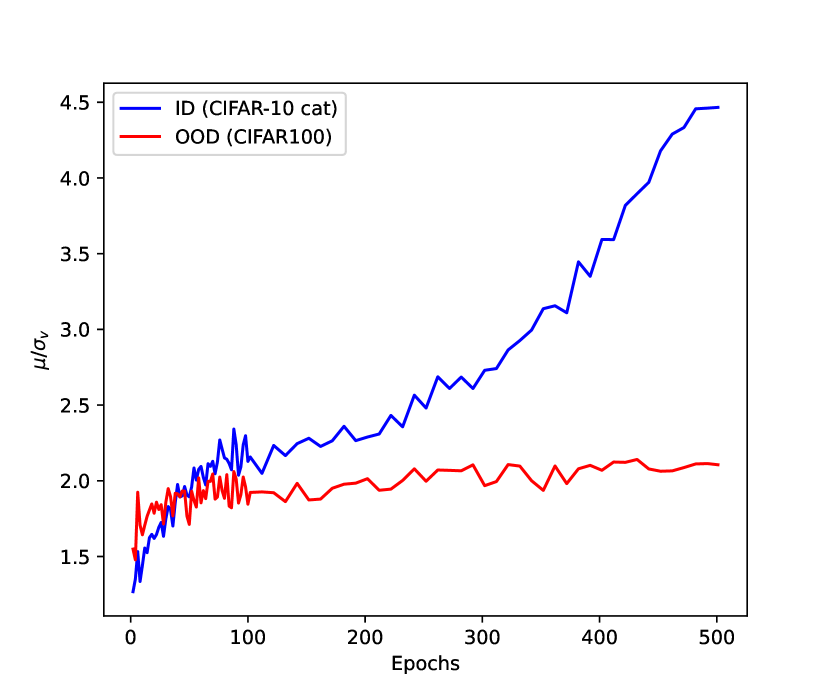
$\mu/\sigma_{v}$

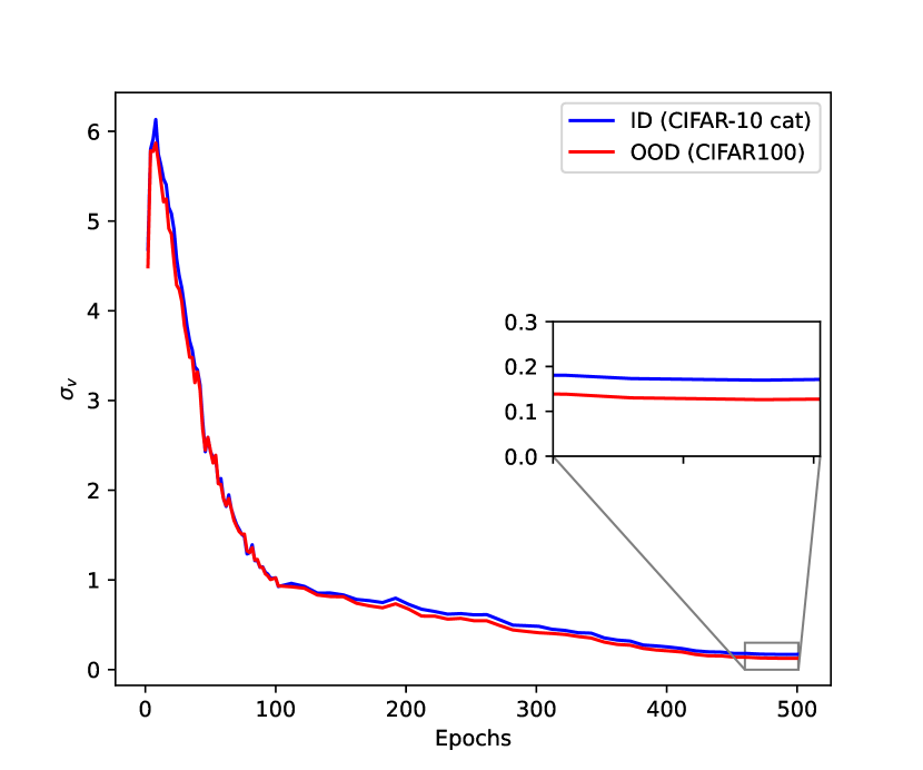
$\sigma_{v}$

Figure 2: Averages of $\mu/\sigma_{v}$ and $\sigma_{v}$ for both normal and OOD samples during the optimization of $\mathcal{L_{\text{contrastive}}}$ using only normal samples. While there is only a minimal difference in $\sigma_{v}$ between normal and OOD samples, the ratio $\mu/\sigma_{v}$ for normal samples becomes significantly larger as the training progresses, empirically supporting the favor of $\mathcal{L}_{\text{contrastive}}$ in increasing $\mu$.

3.3 The $\ell_{2}$-norm of contrastive features: more than an anomaly score

As discussed in Section 3.1, the normalization in contrastive learning inherently promotes a large norm for the contrastive feature of training samples rather than samples from an out-of-distribution dataset; it naturally creates a separation between in-distribution data and out-of-distribution data on the contrastive feature space. Exploiting this characteristic, CSI uses the $\ell_{2}$-norm of contrastive features as a powerful tool for detecting anomalies, which has been experimentally shown to be remarkably effective [36]. Beyond a tool used in inference time, we propose to utilize the $\ell_{2}$-norm as a component in the encoder training process.

Outlier exposure for contrastive learning. Our key finding is that we can further increase this separation by simply forcing the encoder to produce zero-values contrastive features for many augmentations of out-of-distribution samples, thus improving the anomaly detection capabilities. In this paper, we consider a specific out-of-distribution dataset, referred to as outlier exposure dataset, denoted as $\mathcal{D}_{\text{oe}}$. We define the general form of our proposed outlier exposure contrastive learning loss as follows:

$$\mathcal{L}_{\text{oecl}}\triangleq\mathcal{L}_{\text{contrastive}}(z;\tau,M)+\alpha\mathbb{E}_{x\in\mathcal{D}_{\text{oe}},t\in T_{\text{oe}}}\lVert f(t(x))\rVert_{2},$$ (7)

where $\alpha$ is a balancing hyper-parameter, and $T_{\text{oe}}$ is a set of transformations for OE augmentations. Typically, $T_{\text{oe}}$ is set equal to the set of augmentations $T$. $\mathcal{D}_{\text{oe}}$ can either consist of randomly collected images in terms of outlier exposure [15]; [25], or be generated through distributional-shifting transformations as employed in CSI [36]. This versatility allows our proposed approach to be interpreted as an outlier exposure extension for contrastive learning or a fully self-supervised generalization of CSI and SimCLR. Specifically, in the later setting, we consider a family of augmentations $\mathcal{S}_{\text{oe}}$, which we call outlier exposure transformations. These transformations satisfy that for any $S\in\mathcal{S}_{\text{oe}}$, $S(x)$ can be regarded as an outlier with respect to any data joining $\mathcal{L}_{\text{contrastive}}$. It is worth noting that if $\mathcal{L}_{\text{contrastive}}$ is CSI, then $\mathcal{S}_{\text{oe}}$ does not contain any elements from the distribution-shifting transformations $\mathcal{S}$ of CSI, i.e., $\mathcal{S}_{\text{oe}}\cap\mathcal{S}=\varnothing$. The self-outlier-exposure contrastive learning loss is given by,

$$\mathcal{L}_{\text{{oecl}}}=\mathcal{L}_{\text{contrastive}}(z;\tau,M)+\alpha \mathbb{E}_{x\in\mathcal{S}_{\text{oe}}\left(\mathcal{D}\right),t\in T_{\text{oe}}}\lVert f(t(x))\rVert_{2},$$ (8)

$$\text{where}~{}\mathcal{S}_{\text{oe}}\left(\mathcal{D}\right)\triangleq\left\{S(x)\right\}_{S\in\mathcal{S}_{\text{oe}},x\in\mathcal{D}}.$$

Score functions for detecting anomalies. Upon the contrastive feature $f(\cdot)$ learned by our proposed training objective, we define several score functions for deciding whether a given sample $x$ is normal or not. All of our score functions follow the conventional philosophy that in-distribution samples have higher scores. The most obvious choices are $\ell_{2}$-norm of the contrastive feature and its ensembe version over random augmentations.

Non-ensemble $$: s_{\ell_{2}} \triangleq\lVert f(x)\rVert_{2}^{2},$$

Ensemble v1 $$: s_{\ell_{2}-\text{ens}} \triangleq\mathbb{E}_{t\in T}\lVert f(t(x))\rVert_{2}^{2}.$$

Ensemble v2 $$: s_{\mu} \triangleq\lVert\mathbb{E}_{t\in T}f(t(x))\rVert_{2}^{2}.$$ (9)

4 Main Experiments

In this section, we present our results for common unimodal and multimodal benchmarks.

4.1 Implementation Details

In this study, we focus mainly on the outlier-exposure extension setting. Here, we train our models using the objective function (7), where $\mathcal{L}_{\text{contrastive}}$ is SimCLR. We adopt ResNet-18 [13] as the main architecture, and we pre-train our models for 50 epochs using SimCLR. As for data augmentations $T$ and $T_{\text{oe}}$, we follow the ones used by [36]: namely, we apply random crop, horizontal flip, color jitter, and grayscale. We detect OOD samples using the ensemble score function (3.3) with 32 augmentations.

In addition to the outlier-exposure extension, for CIFAR-10 and ImageNet-30 datasets, we also report the results using the fully self-supervised approach, where we train our models using the objective function (8) with CSI as $\mathcal{L}_{\text{contrastive}}$ and rotations as shifting transformations. Specifically, we choose $\mathcal{S}=\left\{\mathbb{I},R_{90}\right\}$ and $\mathcal{S}_{\text{oe}}=\left\{R_{180},R_{270}\right\}$, where $R_{\text{a}}$ is the rotation of $\text{a}^{\circ}$ degree. Apart from this modification, we maintain the other training setups from the above outlier-exposure extension setting. Complete experimental details are available in the appendix E and our code has been open source .

4.2 Datasets

We evaluate our models using the standard CIFAR-10 [19] and ImageNet-30 [10]; [16] datasets. We further conduct our experiments with additional datasets: the aerial dataset DIOR [22] and the microscopy dataset Raabin-WBC [18]. Both of them are symmetry datasets, which are obviously challenging for rotation-based methods like CSI or GT [16]. It is important to clarify that, in this study, the term “non-standard” datasets refers to datasets from domains beyond conventional life photography.

For OE datasets, we use 80 Million Tiny Images (80MTI) [37] for the CIFAR-10 dataset and ImageNet-22k with ImageNet-1k removed for the other datasets. This follows the experimental setup in [16] and [25]. Please refer to the appendix E for more details.

4.3 Benchmarks

We conduct our experiments in two main benchmarks: (1) unimodal and (2) multimodal benchmarks.

Unimodal benchmark. Generally, unimodal is the setting where there is one semantic class in the normal data. Within this study, if not mentioned otherwise, we mostly use the widely popular one vs. rest benchmark [31]; [12]; [15]; [32]; [36]; [35]; [9]; [8]; [29]. This benchmark is constructed based on classification datasets (e.g., CIFAR-10), where “one” class (e.g., “cat”) is considered normal and the “rest” classes (e.g., “dog”, “automobile”, …) are considered anomalous during the test phase. Unless otherwise specified, we use all available classes as our one vs. rest classes.

Multimodal benchmark. We consider a recently and more challenging multimodal benchmark called leave-one-class-out [25]; [8]; [1]. In contrast to the one vs. rest benchmark, the roles are reversed, i.e., the “rest” classes (e.g., “dog”, “automobile”, …) are designated as normal and the “one” class (e.g., “cat”) is abnormal. The presence of multiple semantically different classes as a normal class in this benchmark makes the distribution of normal samples multimodal [25], hence the models are required to learn high-quality deep representations to effectively distinguish between normal and abnormal samples. For all datasets, all available classes are employed as our leave-one-class-out classes. However, due to computation constraints, for ImageNet-30, we randomly select 10 classes as our leave-one-class-out classes. Further details are provided in the appendix F.

Throughout all of our experiments on the unimodal and multimodal benchmarks, we train our models using only the training data of the normal class and samples from an OE set that does not include any classes of the anomaly classes in the original classification datasets. We use the area under the receiver operating characteristic curve (AUC) to quantify detection performance.

4.4 Comparison Methods

Our study focuses on an end-to-end approach, i.e., training from scratch. Therefore, we primarily present results from end-to-end methods that have achieved state-of-the-art performance. In the leave-one-class-out setting, we further consider transfer learning-based methods.

End-to-end methods. We select methods that have demonstrated state-of-the-art performance on the CIFAR-10 and ImageNet-30 unimodal benchmarks.

• Unsupervised: The unsupervised methods we consider include DSVDD [31], vanilla-SimCLR [36], GT+ [16], and CSI [36].

• Unsupervised OE: We present the results from DASD [32], HSC [25] and the unsupervised OE variant of GT+ [16].

• Supervised OE: We report the results from BCE [25], a standard binary cross-entropy classifier, which is optimized to discern samples from the training datasets and the OE datasets. We also report results on the focal loss classifier with $\gamma=2$ [23], which can be found in [25].

Transfer learning-based methods. In the multimodal setting, we additionally explore transfer learning-based methods. For this category, we select the currently top-performing methods, which include DN2 [4], PANDA [29], Transformly [8] and BCE-CL [25]. All methods are unsupervised with the exception of BCE-CL, which is OE-based and supervised. The reported results were either extracted from the original papers, if available, or obtained by conducting experiments following the authors’s publicly available code (where possible).

4.5 Results

Our main results are provided in Table 1 and Table 2.

Table 1: Mean AUC detection performance in $\%$ over 5 trials for end-to-end methods on the CIFAR-10, ImageNet-30, DIOR and Raabin-WBC in unimodal benchmarks. Bold denotes the best results for training-from-scratch methods, and underline denotes the overall best result. $\ast$ denotes results taken from the reference, $\natural$ denotes results taken from [29]

	Unsupervised				Unsupervised OE				Supervised OE
	SimCLR	GT+	CSI	self-OECL	$\text{GT+}^{\ast}$	$\text{DASD}^{\ast}$	HSC	OECL	$\text{Focal}^{\ast}$	BCE
CIFAR-10	$86.1$	$90.1^{\ast}$	$94.3^{\ast}$	94.7	95.6	$94.5$	$95.9^{\ast}$	97.8	95.8	$96.1^{\ast}$
ImageNet-30	64.8	$84.8^{\ast}$	$91.6^{\ast}$	87.3	85.7	$96.7$	$97.3^{\ast}$	$\underline{\bm{97.7}}$	97.5	$\underline{\bm{97.7}}^{\ast}$
DIOR	$72.8$	$73.3^{\natural}$	$78.5^{\natural}$	$\times$	$\times$	$\times$	89.2	$\underline{\bm{91.1}}$	$\times$	88.5
Raabin-WBC	85.9	$\times$	62.3	$\times$	$\times$	$\times$	60.6	$\underline{\bm{88.6}}$	$\times$	66.5

Table 2: Mean AUC detection performance in $\%$ over 2 trials for methods on the CIFAR-10, ImageNet-30, DIOR and Raabin-WBC in multimodal benchmarks. Bold denotes the best results for training-from-scratch methods, and underline denotes the overall best result. $\ast$ denotes results taken from the reference, $\natural$ denotes results taken from [8].

	Unsupervised					Unsupervised OE		Supervised OE
	DSVDD	SimCLR	$\text{DN2}^{\ast}$	$\text{PANDA}^{\ast}$	$\text{Transformly}^{\ast}$	HSC	OECL	BCE	$\text{BCE-CL}^{\ast}$
	$\checkmark$	$\checkmark$				$\checkmark$	$\checkmark$	$\checkmark$
CIFAR-10	$50.7^{\natural}$	$83.9$	$71.7$	$78.5$	$90.4$	$84.8^{\ast}$	$\bm{94.6}$	$86.6^{\ast}$	$\underline{98.4}$
ImageNet-30	$\times$	$94.8$	$\times$	$\times$	$\times$	$86.7^{\ast}$	$\bm{98.8}$	$86.5^{\ast}$	$\underline{99.2}$
DIOR	$56.7^{\natural}$	$\underline{\bm{87.7}}$	$81.1$	$86.9$	$66.7$	$55.5$	$87.3$	$62.5$	$\times$
Raabin-WBC	$\times$	$\underline{\bm{83.6}}$	$\times$	$\times$	$\times$	$61.4$	$82.2$	$62.1$	$\times$

4.6 Analysis

Overall, our proposed methods achieve performance comparable to the current state-of-the-art methods and mostly outperform training-from-scratch approaches. A particularly surprising outcome is that our self-OECL surpasses CSI in the CIFAR-10 one vs. rest benchmark, while also obtaining decent performance in ImageNet-30. These results support our principles that enhancing the separation of normal and OOD samples in the contrastive feature space is beneficial for OOD detection. Furthermore, this property holds promising potential for future advancements in fully unsupervised OOD detection methods, particularly when more sophisticated OOD generation techniques are introduced (e.g., the SDE-based method [27]), transcending the limitations of rotations.

The benefits of OE datasets. Our OECL significantly enhances OOD detection compared to the baseline SimCLR in nearly all benchmarks, showcasing substantial improvements. The benefits of “anomalousness” from OE are especially evident for the non-standard datasets. Notably, the performance of state-of-the-art CSI, as expected, shows minimal improvement and even degradation, with AUC scores of $78.5\%$ for DIOR and $62.3\%$ for Raabin-WBC, respectively. This is due to the fact that applying rotations no longer shifts the distribution of symmetry image datasets like DIOR and Raabin-WBC, which is the fundamental assumption of CSI. In contrast, OECL achieves higher scores of $92.0\%$ and $88.8\%$ for these datasets, which indicates the effectiveness of incorporating OE when working with non-standard datasets.

The power of contrastive learning. As reported in [25] and further supported by our experiments, there are situations where the current OE techniques struggle, such as the leave-one-class-out benchmark or non-standard training datasets. Particularly in the leave-one-class-out benchmark, where the training dataset’s distribution is multimodal, the strategy of encouraging the concentration of normal representations used in HSC is ineffective, leading to suboptimal performance. Our proposed OECL, on the other hand, outperforms the majority of unsupervised methods, including those that used trained features in the multimodal setting, as shown in Table 2. Notably, OECL achieved a remarkable AUC score of $98.8\%$ for the rich and diversified ImageNet-30, falling behind OE transfer learning-based BCE-CL by only $0.4\%$. These outcomes imply that, in contrast to HSC and BCE, the ability of OECL to exploit high-quality features through contrastive learning is especially advantageous in the context of multimodal datasets, particularly those that are rich and diverse. To further illustrate the strengths of contrastive learning in OECL, we measure the performance of OE methods with SVHN, a non-standard image dataset, as our OE. Table 3 shows the overwhelming performance of OECL over HSC.

Table 3: Mean AUC detection performance in $\%$ over 5 trials for OECL and HSC on the one vs. rest CIFAR-10 benchmark.

Dataset	OE Dataset	OECL	HSC
CIFAR-10	SVHN	$\bm{92.2}$	54.2

Taken together, these above results support our principles on integrating contrastive learning with OE datasets.

5 Few-shot OOD Detection

In this section, we explore the generalization of OECL to unseen anomalies. In many real-life scenarios, we are able to collect some samples of a few specific classes of anomalies, which we term as “obtainable OOD classes”. For instance, in hematology, suppose that neutrophils, representing about $60\%$ of circulating white blood cells, are regarded as normal samples, while white blood cells of other types are considered anomalies. Within this setting, lymphocytes, which make up about $30\%$ of white blood cells, can be considered an obtainable OOD class, and other white blood cells like basophils ($\approx 1\%$) and eosinophils ($\approx 3\%$) represent “unseen anomalies”.

Few-shot OOD benchmark. Inspired by [34] and [43], to evaluate OOD detection performance against unseen anomalies described above, we introduce the “few-shot OOD” benchmark. This benchmark is constructed using classification datasets (e.g., Raabin-WBC), where the class with the largest number of samples (neutrophils) is considered as normal. The next largest class (lymphocytes) is selected as the obtainable OOD class, for which a small number of samples are available during training. All other classes (basophils, eosinophils, and monocytes) serve as unseen anomalies. At inference time, the goal is to identify normal samples and unseen abnormal samples. In this study, we focus on the extreme case one-shot and ten-shot detection, implying access to only a single sample and ten samples, respectively. To some degree, the few-shot OOD benchmark represents unimodal benchmarks with very few standard OE samples.

Datasets. In addition to the Raabin-WBC dataset, we use the HAM10000 dataset [38] which is a collection of dermatoscopic images of common pigmented skin lesions.

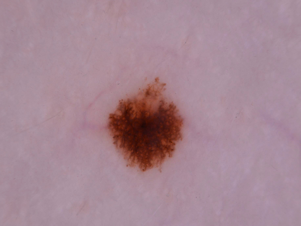
Melanocytic nevi
(normal)

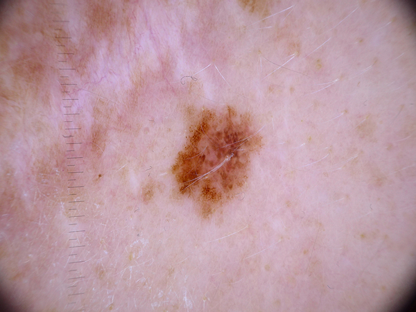
Melanoma
(obtainable OOD)

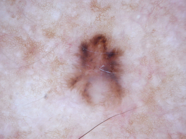
Basal cell carcinoma
(unseen OOD)

Figure 3: Examples of normal, obtainable OOD and unseen OOD images from Ham10000 dataset.

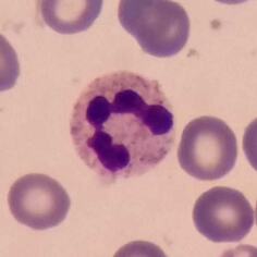
Neutrophils
(normal)

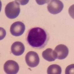
Lymphocytes
(obtainable OOD)

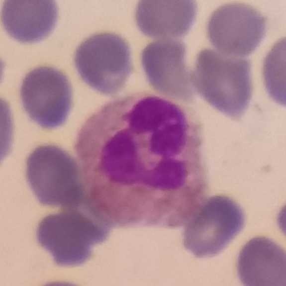
Lymphocytes
(unseen OOD)

Figure 4: Examples of normal, obtainable OOD and unseen OOD images from Raabin-WBC.

Results and discussion. Results from Table 7 show that exposing OECL to a small number of samples from a specific near-OOD class helps improve anomaly detection accuracy significantly. For less diverse Raabin-WBC, only one single OOD sample helps to boost the AUC score up about $9\%$. These results suggest a practical solution in which a limited number of OOD samples [21]; [42], are integrated into the training phase to improve AD performance.

Table 4: Mean AUC detection performance in $\%$ of OECL over 5 trials on the Raabin-WBC and HAM1000 few-shot OOD benchmarks.

Dataset	Normal Class	OE	Method	# Samples
				k=0	k=1	k=10	Full-shot
Raabin-WBC	Neutrophils	Lymphocytes	OECL	68.1	$\bm{76.9}$	$\bm{79.9}$	83.6
			BCE	$\times$	49.0	72.6	$\bm{95.0}$
			HSC	$\times$	64.7	69.1	86.1
HAM10000	Melanocytic nevi	Melanoma	OECL	63.2	$\bm{65.6}$	$\bm{69.4}$	$\bm{83.9}$
			BCE	$\times$	61.7	60.4	79.1
			HSC	$\times$	64.1	46.0	75.6
HAM10000	Melanocytic nevi	Benign keratosis	OECL	59.3	61.6	$\bm{69.4}$	85.7
			BCE	$\times$	53.2	54.3	84.8
			HSC	$\times$	$\bm{64.7}$	69.1	$\bm{88.0}$

6 Conclusion

We propose an easy-to-use but effective technique named outlier exposure contrastive learning, which extends the robustness and strengths of both contrastive learning and OE for out-of-distribution detection problems. OECL demonstrates strong and outstanding performance under various OOD detection scenarios. We believe our work will serve as an essential baseline for future OOD detection and self-supervised learning.

Broader impact

This study focuses on the domain of out-of-distribution (OOD) detection, which is a crucial part of trustworthy intelligent systems. Our research offers both theoretical and empirical findings regarding the behavior of $\ell_{2}$-norm in contrastive learning. Additionally, we propose a simple technique for directly incorporating OOD samples into contrastive learning methods. By leveraging “anomalousness” of OOD samples and high-quality representations of contrastive learning, our work will give provide a feasible solution to problems where current OE and contrastive AD methods fail. We expect that these results will have an impact on real-life applications as well as academic advancements, leading to the development of safer and more dependable AI systems.

Appendix A Proof of Figure 1

Lemma 1.

For any $\mu>0$, $f(y)$ is a non-increasing and convex function on $\left[0,\infty\right)$ where

$$f(y)=\int_{-\infty}^{\infty}\frac{x}{\sqrt{x^{2}+y}}e^{-(x-\mu)^{2}/2\sigma^{2}}dx$$

Proof.

Firstly, rewrite

$$f(y) =\int_{0}^{\infty}+\int_{-\infty}^{0}\frac{x}{\sqrt{x^{2}+y}}e^{-(x-\mu)^{2}/2\sigma^{2}}dx$$

$$=\int_{0}^{\infty}\frac{x}{\sqrt{x^{2}+y}}\left(e^{-(x-\mu)^{2}/2\sigma^{2}}-e^{-(x+\mu)^{2}/2\sigma^{2}}\right)dx$$

$$=\int_{0}^{\infty}\frac{x}{\sqrt{x^{2}+y}}e^{-(x+\mu)^{2}/2\sigma^{2}}\left(e^{2x\mu/\sigma^{2}}-1\right)dx$$

$f^{\prime}(y)$ and $f^{\prime\prime}(y)$ given by

$$f^{\prime}(y) =\left(\int_{0}^{\infty}\frac{x}{\sqrt{x^{2}+y}}e^{-(x+\mu)^{2}/2\sigma^{2}}\left(e^{2x\mu/\sigma^{2}}-1\right)dx\right)_{y}^{\prime}$$

$$=\int_{0}^{\infty}\left(\frac{x}{\sqrt{x^{2}+y}}\right)_{y}^{\prime}e^{-(x+\mu)^{2}/2\sigma^{2}}\left(e^{2x\mu/\sigma^{2}}-1\right)dx$$

$$=\int_{0}^{\infty}\frac{-x}{2(x^{2}+y)^{3/2}}e^{-(x+\mu)^{2}/2\sigma^{2}}\left(e^{2x\mu/\sigma^{2}}-1\right)dx$$

$$f^{\prime\prime}(y) =\left(\int_{0}^{\infty}\frac{x}{\sqrt{x^{2}+y}}e^{-(x+\mu)^{2}/2\sigma^{2}}\left(e^{2x\mu/\sigma^{2}}-1\right)dx\right)_{y}^{\prime\prime}$$

$$=\int_{0}^{\infty}\left(\frac{x}{\sqrt{x^{2}+y}}\right)_{y}^{\prime\prime}e^{-(x+\mu)^{2}/2\sigma^{2}}\left(e^{2x\mu/\sigma^{2}}-1\right)dx$$

$$=\int_{0}^{\infty}\frac{3x}{(x^{2}+y)^{5/2}}e^{-(x+\mu)^{2}/2\sigma^{2}}\left(e^{2x\mu/\sigma^{2}}-1\right)dx$$

Since $e^{2x\mu/\sigma^{2}}\geq 1~{}\forall x>0$, it’s clear that $f^{\prime}(y)<0$ and $f^{\prime\prime}(y)>0$, i.e, $f(y)$ is non-increase and convex over $\left[0,\infty\right)$. ∎

Appendix B Gradual reduction of $\ell_{2}$-norm of contrastive features

In this section, to study the effect of alignment and uniformity on the $\ell_{2}$-norm of contrastive features, we use the contrastive learning framework proposed by [40],

$$\mathcal{L}_{\text{contrastive}}=\mathcal{L}_{\text{align}}+\mathcal{L}_{\text{uniform}},$$

where

$$\mathcal{L}_{\text{align}} =\underset{(x,y)\sim p_{\text{pos}}}{\mathbb{E}}\left[\|z(x)-z(y)\|_{2}^{2}\right],$$ (10)

$$\mathcal{L}_{\text{uniform}} =\log\underset{\begin{subarray}{c}(x,y)\overset{\text{i.i.d}}{\sim}p_{\text{data}}\end{subarray}}{\mathbb{E}}\left[e^{-\|z(x)-z(y)\|_{2}^{2}}\right].$$ (11)

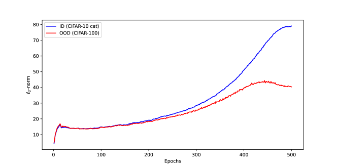
Figure 5: $\ell_{2}$-norm of contrastive features for both normal and OOD samples during optimization of $\mathcal{L}_{\text{contrastive}}$ without $\ell_{2}$-normalization, using only normal samples.

Necessity of cosine similarity. Figure 5 depicts the $\ell_{2}$-norm of contrastive features during optimization of $\mathcal{L}_{\text{contrastive}}$ using Euclidean distance, i.e., $z(x)=f(x)$. As expected, without $\ell_{2}$-normalization, the $\ell_{2}$-norm of contrastive features $f(x)$ does not exhibit the characteristic of gradual decrease but rather increases as training progresses. This shows the critical role played by cosine similarity in driving the gradual reduction of the $\ell_{2}$-norm of contrastive features.

(a) $\ell_{2}$-norm of contrastive features.

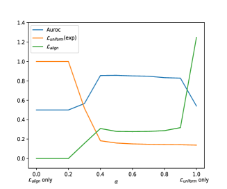
(b) $\mathcal{L}_{\text{align}},\mathcal{L}_{\text{uniform}}$ and AUC score.

Figure 6: Impact of optimizing different weighted combinations of $\mathcal{L}_{\text{align}}$ and $\mathcal{L}_{\text{uniform}}$, trained on CIFAR-10 cat class. $\mathcal{L}_{\text{uniform}}$ is exponentiated for visualization.

Necessity of both alignment and uniformity. Figure 6 shows how the AUC score and the $\ell_{2}$-norm change in response to optimizing differently weighted combinations $(1-\alpha)\mathcal{L}_{\text{align}}+\alpha\mathcal{L}_{\text{uniform}}$. Similar to the accuracy curve in [40], AUC score curve of OOD detection is also inverted-U-shaped. This means that both alignment and uniformity are vital for a high-quality features extractor, hence is necessity for a good OOD detector. When $\mathcal{L}_{\text{align}}$ is weighted much higher than $\mathcal{L}_{\text{uniform}}$, degenerate solution occurs and all inputs (including normal and OOD samples) are mapped to the same point ($\exp(\mathcal{L}_{\text{uniform}})$=1). However, as long as the ratio between two weights is not too large (e.g., $0.4\leq\alpha\leq 0.9$), we consistently observe both the gap between the $\ell_{2}$-norm of normal and OOD contrastive representations and their gradual reduction as training progresses. An intriguing observation is the relation between $\alpha$ and the $\ell_{2}$-norm of OOD samples; as the value of $\alpha$ increases, the $\ell_{2}$-norm of OOD contrastive features decreases proportionally. This suggests that uniformity plays a more significant role in the gradual reduction of $\ell_{2}$-norm of contrastive features. We hope that future research will offer a more in-depth understanding of the fundamental cause of this phenomenon.

Appendix C Anomaly detection scores

Theoretically, under the assumptions of fig. 1, ensemble versions of our anomaly detection score satisfy,

$$s_{\mu} =\mu^{2}$$ (12)

$$s_{\ell_{2}-\text{ens}} =\mu^{2}+\sigma^{2}+\sigma_{V}^{2}$$ (13)

Experimentally, we find that the overall detection performance of $s_{\mu}$ is better, especially for non-standard datasets as shown in table 5.

Table 5: AUC detection performance in $\%$ using $s_{\ell_{2}}$, $s_{\ell_{2}-\text{ens}}$ and $s_{\mu}$.

Dataset	Benchmark	$s_{\mu}$	$s_{\ell_{2}-\text{ens}}$	$s_{\ell_{2}}$
DIOR	unimodal	$\bm{91.1}$	90.7	90.8
	multimodal	$\bm{87.3}$	86.9	87.1
Raabin-WBC	unimodal	$\bm{88.6}$	88.4	$\bm{88.6}$
	multimodal	$\bm{82.2}$	82.0	81.4

In [36], it was demonstrated that cosine similarity to the nearest sample and contrastive feature norm are complementary, resulting in additional improvements. While we have observed a similar phenomenon in our experiments, where the combination of cosine similarity and feature norm mostly yields the best results, it may not exhibit absolute consistency across various scenarios, as indicated in Table 6. Furthermore, we wish to emphasize the effectiveness of the $\ell_{2}$-norm in anomaly detection. Therefore, we have chosen to present our anomaly score without the inclusion of cosine similarity.

Table 6: AUC detection performance in $\%$ using $s_{\mu}$ and $\text{sim}+s_{\mu}$.

Dataset	Benchmark	OE	$s_{\mu}$	$\text{sim}+s_{\mu}$
Raabin-WBC	unimodal		${85.9}$	$\bm{88.1}$
Raabin-WBC	unimodal	✓	${88.6}$	$\bm{89.0}$
DIOR	unimodal		$72.8$	$\bm{74.9}$
DIOR	unimodal	✓	$91.1$	$\bm{91.2}$
CIFAR-10	unimodal		${86.1}$	$\bm{86.8}$
CIFAR-10	unimodal	✓	$\bm{97.8}$	${97.7}$
ImageNet-30	unimodal		${64.8}$	$\bm{66.7}$
ImageNet-30	unimodal	✓	$\bm{97.7}$	$97.5$

Appendix D Small datasets

Due to the fact that OECL relies on contrastive representation learning to extract high-quality features, it does not perform well on datasets where its contrastive learning module is unable to learn strong features and OE is not informative. This is particularly evident in scenarios where the training datasets are small and non-standard. To illustrate this, we use the DTD [7] one vs. rest benchmark and the recent manufacturing dataset MVTec-AD [5], with ImagetNet22k serving as the OE dataset.

DTD is a dataset that includes different classes of textures. Comprising 15 distinct classes of manufacturing objects (such as screws, cables, and capsules), MVTec-AD presents both normal and abnormal samples for each class. For example, a screw class consists of two sets of images: a training set of images of typical screws, and a test set of images of typical screws, along with images of screws with anomalous defects. Both DTD and MVtec-AD consist of fewer than 40 samples for each normal class. Table 7 shows the results of OECL on these small datasets.

Table 7: Mean AUC detection performance in $\%$ over 5 trials on the DTD one vs. rest and on the MVTec-AD benchmarks with ImageNet1k OE.

Dataset	OECL	$\text{HSC}^{\ast}$	$\text{BCE}^{\ast}$
DTD	65.6	72.7	$\bm{73.3}$
MVTec-AD	62.1	$\bm{70.1}$	66.1

As anticipated, OECL results more poorly on the small datasets than state-of-the-art methods: OECL scores around $62\%$ while [3] and [30] score above $99\%$ AUC for the MVTec-AD benchmark. These results indicate that for small datasets, OECL may not be the optimal choice.

Appendix E Experimental details

E.1 Implementation details

We use Resnet [13] along with a 2-layer MLP with batch-normalization and Relu after the first layer. The based contrastive learning module is SimCLR (1) with a temperature of $\tau=0.5$. We set the balancing hyperparameter $\alpha=1$ for CIFAR-10 and Imagenet-30 datasets and $\alpha=0.1$ for DIOR, Raabin-WBC, and HAM10000 datasets. For optimization, we train all models with 500 epochs under LARS optimizer [41] with a weight decay of $1e-6$ and momentum of $0.9$. During the first 50 epochs, we set $\alpha=0$ as a warming-up phase. For the learning rate scheduling, we use learning rate 0.1 and decay with a cosine decay schedule without restart [26]. We use the batch size of 256 for both normal and OE samples during training, and we detect OOD samples using the ensemble score function (8) with 32 augmentations. Additionally, we implement global batch normalization [17], which shares batch normalization parameters across GPUs in distributed training setups.

E.2 Datasets

• CIFAR-10 includes 10 standard object classes with totally $50000$ images for training and $10000$ images for testing.

• ImageNet-30 contains $39000$ training and $3000$ testing images that are divided equally into $30$ standard object classes.

• DIOR is an aerial images dataset with 19 object categories. Following previous papers [8]; [29], we use the bounding box provided with the data, and select classes that have more than 50 images with dimensions greater than $120\times 120$ pixels. This preprocessing step results in 19 classes, with an average of 649 samples. The class sizes are not equal, with the smallest class (baseballfield) in the training set containing 116 samples and the largest (windmill) containing 1890 samples.

• Raabin-WBC is a dataset comprising images of white blood cells (WBCs) categorized into five classes. The training set contains more than $10000$ images. For the test set, we choose the Test-A of the dataset [18].

• HAM10000 is a large collection of dermatoscopic images of common pigmented skin lesions with total $10000$ training images. We follow the instruction given by [38], using ISIC2018_Task3_Test_Images.zip (1511 images) for the evaluation purposes.

E.3 Data augmentations

For data augmentations $T$ and $T_{\text{oe}}$, we use SimCLR augmentations: random crop, horizontal flip, color jitter, and grayscale. We simply set $T_{\text{oe}}=T$ in all our experiments. The details for the augmentations are:

• Random crop. We randomly crops of the original image with uniform distribution from $a$ to $1.0$. We select $a=0.5$ for Raabin-WBC dataset and Ham10000 dataset, and all the other datasets we set $a=0.08$. After cropping, cropped image are resized to match the original image size.

• Horizontal flip. All training images are randomly horizontally flipped with $50\%$ of probability.

• Color jitter. Color jitter changes the brightness, contrast, saturation and hue of images. We implement color jitter using pytorch’s color jitter function with $\text{brightness}=0.4,\text{contrast}=0.4,\text{saturation}=0.4$ and $\text{hue}=0.1$. The probability to apply color jitter to a training image is set at $80\%$.

• Grayscale. Convert an image to grayscale with $20\%$ of probability.

Appendix F Results on individual classes

We report results of our experiments over all classes in the main paper in this section.

F.1 Unimodal benchmark

Table 8: Mean AUC detection performance in $\%$ for all individual classes on the CIFAR-10 one vs. rest benchmark from section 4.5.

Class	SimCLR	self-OECL	OECL
Airplane	81.6	88.0	97.6
Automobile	97.1	99.0	99.5
Bird	88.5	93.6	96.9
Cat	80.4	89.8	94.0
Deer	80.6	94.7	97.2
Dog	85.5	92.6	96.8
Frog	84.6	96.6	99.3
Horse	91.4	98.5	98.8
Ship	88.3	98.3	99.1
Truck	82.8	96.1	98.5
Mean AUC	86.1	94.7	97.8

Table 9: Mean AUC detection performance in $\%$ for all individual classes on the ImageNet-30 one vs. rest benchmark from section 4.5.

Class	SimCLR	self-OECL	OECL
Acorn	61.8	84.0	98.9
Airliner	82.1	98.2	99.8
Ambulance	96.9	98.9	100
American alligator	49.4	86.8	98.4
Banjo	60.7	84.8	96.9
Barn	52.3	98.6	98.7
Bikini	72.8	95.8	97.9
Digital clock	42.8	66.4	97.8
Dragonfly	69.7	90.9	97.9
Dumbbell	59.2	80.9	91.3
Forklift	74.7	95.8	98.4
Goblet	61.2	91.0	96.7
Grand piano	70.8	94.7	98.3
Hotdog	68.3	84.9	97.7
Hourglass	73.5	92.5	98.9
Manhole cover	78.7	73.3	100
Mosque	91.3	99.1	99.1
Nail	69.9	66.8	93.8
Parking meter	51.3	94.8	95.3
Pillow	59.5	67.2	95
Revolver	79.6	95.6	98.1
Rotary dial telephone	46.1	83.0	98.6
Schooner	75.1	98.7	99
Snowmobile	61.7	97.3	99.1
Soccer ball	71.9	71.5	96.7
Stingray	47.3	78.7	99.4
Strawberry	66.2	80.4	99
Tank	70.5	93.4	97.9
Toaster	43.8	76.1	91.9
Volcano	50.8	97.4	99.1
Mean AUC	64.8	87.3	97.7

Table 10: Mean AUC detection performance in $\%$ for all individual classes on the DIOR one vs. rest benchmark from section 4.5.

Class	SimCLR	HSC	OECL	BCE
Airplane	65.5	89.7	87.3	88.9
Airport	57.5	96.6	94.7	92.3
Baseball field	87.6	96.3	90.2	98.0
Basketball court	60.0	82.6	89.3	81.3
Bridge	85.7	96.2	94.9	96.1
Chimney	82.5	94.1	90.5	93.3
Dam	80.2	82.1	94.4	71.2
Expressway service area	82.2	96.8	90.8	98.1
Expressway toll station	67.1	75.8	90.8	72.9
Golf field	56.3	97.0	96.1	95.2
Ground track field	87.6	90.3	95.7	92.2
Harbor	81.9	91.0	95.0	92.2
Overpass	76.3	87.6	85.8	82.9
Ship	61.0	80.0	85.7	73.4
Stadium	82.6	88.2	93.0	95.5
Storage tank	53.3	96.1	95.6	95.9
Tennis court	92.0	90.2	95.4	92.4
Train station	67.3	70.1	86.1	75.8
Windmill	55.7	94.6	79.5	94.7
Mean AUC	72.8	89.2	91.1	88.5

Table 11: Mean AUC detection performance in $\%$ for all individual classes on the Raabin-WBC one vs. rest benchmark from section 4.5.

Class	SimCLR	HSC	OECL	BCE
Basophil	97.6	95.2	95.9	88.4
Eosinophil	70.1	53.2	70.9	46.8
Lymphocyte	92.3	49.4	98.3	70.2
Monocyte	89.8	50.6	89.8	80.3
Neutrophil	79.9	54.4	88.0	46.8
Mean AUC	85.9	60.6	88.6	66.5

F.2 Multimodal benchmark

Table 12: Mean AUC detection performance in $\%$ for all individual classes on the CIFAR-10 leave-one-class-out benchmark from section 4.5.

Class	SimCLR	OECL
Airplane	90.0	93.5
Automobile	79.4	95.7
Bird	86.3	95.7
Cat	83.5	95.4
Deer	85.1	93.6
Dog	71.8	93.2
Frog	86.9	98.9
Horse	75.9	89.4
Ship	93.4	93.6
Truck	86.1	96.8
Mean AUC	83.9	94.6

Table 13: Mean AUC detection performance in $\%$ for all individual classes on the ImageNet-30 leave-one-class-out benchmark from section 4.5.

Class	SimCLR	OECL
Banjo	90.9	98.2
Barn	97.4	98.5
Dumbbell	91.1	99.1
Forklift	93.3	98.5
Nail	93.1	97.8
Parking meter	95.4	99.0
Pillow	97.7	99.0
Schooner	98.8	98.7
Tank	94.4	99.6
Toaster	95.7	99.2
Mean AUC	94.8	98.8

Table 14: Mean AUC detection performance in $\%$ for all individual classes on the DIOR leave-one-class-out benchmark from section 4.5.

Class	SimCLR	HSC	OECL	BCE
Airplane	94.4	51.7	94.8	73.7
Airport	95.6	81.5	92.8	90.0
Baseball field	96.8	40.4	95.2	62.2
Basketball court	95.7	34.8	96.3	69.5
Bridge	96.2	68.7	94.7	55.0
Chimney	90.0	60.0	82.4	36.5
Dam	67.4	52.3	63.3	45.8
Expressway service area	97.7	65.6	99.4	74.9
Expressway toll station	94.2	52.0	95.1	62.3
Golf field	97.1	32.5	99.1	57.9
Ground track field	83.6	39.2	86.5	51.7
Harbor	74.3	43.1	83.5	41.0
Overpass	53.6	58.9	50.7	49.3
Ship	91.4	68.7	90.9	71.6
Stadium	84.3	43.9	83.8	53.1
Storage tank	94.6	78.0	94.1	74.9
Tennis court	66.4	61.3	60.2	45.3
Trainstation	94.2	52.5	97.5	83.2
Windmill	98.5	69.9	97.7	89.4
Mean AUC	87.7	55.5	87.3	62.5

Table 15: Mean AUC detection performance in $\%$ for all individual classes on the Raabin-WBC leave-one-class-out benchmark from section 4.5.

Class	SimCLR	HSC	OECL	BCE
Basophil	94.0	97.8	94.1	98.4
Eosinophil	67.2	42.7	64.3	64.0
Lymphocyte	98.4	69.5	91.9	26.2
Monocyte	81.4	47.3	89.0	66.8
Neutrophil	77.2	49.9	71.6	55.3
Mean AUC	83.6	61.4	82.2	62.1

References

- Ahmed and Courville [2020] F. Ahmed and A. Courville. Detecting semantic anomalies. Proceedings of the AAAI Conference on Artificial Intelligence, 34(04):3154–3162, Apr. 2020. doi: 10.1609/aaai.v34i04.5712. URL https://ojs.aaai.org/index.php/AAAI/article/view/5712.
- Bachman et al. [2019] P. Bachman, R. D. Hjelm, and W. Buchwalter. Learning Representations by Maximizing Mutual Information across Views. Curran Associates Inc., Red Hook, NY, USA, 2019.
- Batzner et al. [2023] K. Batzner, L. Heckler, and R. König. Efficientad: Accurate visual anomaly detection at millisecond-level latencies, 2023.
- Bergman et al. [2020] L. Bergman, N. Cohen, and Y. Hoshen. Deep nearest neighbor anomaly detection. CoRR, abs/2002.10445, 2020. URL https://arxiv.org/abs/2002.10445.
- Bergmann et al. [2019] P. Bergmann, M. Fauser, D. Sattlegger, and C. Steger. Mvtec ad — a comprehensive real-world dataset for unsupervised anomaly detection. In 2019 IEEE/CVF Conference on Computer Vision and Pattern Recognition (CVPR), pages 9584–9592, 2019. doi: 10.1109/CVPR.2019.00982.
- Chen et al. [2020] T. Chen, S. Kornblith, M. Norouzi, and G. Hinton. A simple framework for contrastive learning of visual representations. In H. D. III and A. Singh, editors, Proceedings of the 37th International Conference on Machine Learning, volume 119 of Proceedings of Machine Learning Research, pages 1597–1607. PMLR, 13–18 Jul 2020. URL https://proceedings.mlr.press/v119/chen20j.html.
- Cimpoi et al. [2014] M. Cimpoi, S. Maji, I. Kokkinos, S. Mohamed, and A. Vedaldi. Describing textures in the wild. In 2014 IEEE Conference on Computer Vision and Pattern Recognition, pages 3606–3613, 2014. doi: 10.1109/CVPR.2014.461.
- Cohen and Avidan [2022] M. J. Cohen and S. Avidan. Transformaly - two (feature spaces) are better than one. In 2022 IEEE/CVF Conference on Computer Vision and Pattern Recognition Workshops (CVPRW), pages 4059–4068, 2022. doi: 10.1109/CVPRW56347.2022.00451.
- Deecke et al. [2021] L. Deecke, L. Ruff, R. A. Vandermeulen, and H. Bilen. Transfer-based semantic anomaly detection. In M. Meila and T. Zhang, editors, Proceedings of the 38th International Conference on Machine Learning, volume 139 of Proceedings of Machine Learning Research, pages 2546–2558. PMLR, 18–24 Jul 2021. URL https://proceedings.mlr.press/v139/deecke21a.html.
- Deng et al. [2009] J. Deng, W. Dong, R. Socher, L.-J. Li, K. Li, and L. Fei-Fei. Imagenet: A large-scale hierarchical image database. In 2009 IEEE Conference on Computer Vision and Pattern Recognition, pages 248–255, 2009. doi: 10.1109/CVPR.2009.5206848.
- Dosovitskiy et al. [2014] A. Dosovitskiy, J. T. Springenberg, M. Riedmiller, and T. Brox. Discriminative unsupervised feature learning with convolutional neural networks. In Z. Ghahramani, M. Welling, C. Cortes, N. Lawrence, and K. Weinberger, editors, Advances in Neural Information Processing Systems, volume 27. Curran Associates, Inc., 2014. URL https://proceedings.neurips.cc/paper_files/paper/2014/file/07563a3fe3bbe7e3ba84431ad9d055af-Paper.pdf.
- Golan and El-Yaniv [2018] I. Golan and R. El-Yaniv. Deep anomaly detection using geometric transformations. In S. Bengio, H. Wallach, H. Larochelle, K. Grauman, N. Cesa-Bianchi, and R. Garnett, editors, Advances in Neural Information Processing Systems, volume 31. Curran Associates, Inc., 2018. URL https://proceedings.neurips.cc/paper_files/paper/2018/file/5e62d03aec0d17facfc5355dd90d441c-Paper.pdf.
- He et al. [2016] K. He, X. Zhang, S. Ren, and J. Sun. Deep residual learning for image recognition. In 2016 IEEE Conference on Computer Vision and Pattern Recognition (CVPR), pages 770–778, 2016. doi: 10.1109/CVPR.2016.90.
- He et al. [2020] K. He, H. Fan, Y. Wu, S. Xie, and R. Girshick. Momentum contrast for unsupervised visual representation learning. In 2020 IEEE/CVF Conference on Computer Vision and Pattern Recognition (CVPR), pages 9726–9735, 2020. doi: 10.1109/CVPR42600.2020.00975.
- Hendrycks et al. [2019a] D. Hendrycks, M. Mazeika, and T. Dietterich. Deep anomaly detection with outlier exposure. In International Conference on Learning Representations, 2019a. URL https://openreview.net/forum?id=HyxCxhRcY7.
- Hendrycks et al. [2019b] D. Hendrycks, M. Mazeika, S. Kadavath, and D. Song. Using self-supervised learning can improve model robustness and uncertainty. In H. Wallach, H. Larochelle, A. Beygelzimer, F. d'Alché-Buc, E. Fox, and R. Garnett, editors, Advances in Neural Information Processing Systems, volume 32. Curran Associates, Inc., 2019b. URL https://proceedings.neurips.cc/paper_files/paper/2019/file/a2b15837edac15df90721968986f7f8e-Paper.pdf.
- Ioffe and Szegedy [2015] S. Ioffe and C. Szegedy. Batch normalization: Accelerating deep network training by reducing internal covariate shift. In F. Bach and D. Blei, editors, Proceedings of the 32nd International Conference on Machine Learning, volume 37 of Proceedings of Machine Learning Research, pages 448–456, Lille, France, 07–09 Jul 2015. PMLR. URL https://proceedings.mlr.press/v37/ioffe15.html.
- Kouzehkanan et al. [2022] Z. M. Kouzehkanan, S. Saghari, S. Tavakoli, P. Rostami, M. Abaszadeh, F. Mirzadeh, E. S. Satlsar, M. Gheidishahran, F. Gorgi, S. Mohammadi, and R. Hosseini. A large dataset of white blood cells containing cell locations and types, along with segmented nuclei and cytoplasm. Scientific Reports, 12(1):1123, 2022. doi: 10.1038/s41598-021-04426-x. URL https://doi.org/10.1038/s41598-021-04426-x.
- Krizhevsky [2009] A. Krizhevsky. Learning multiple layers of features from tiny images. 2009.
- Li et al. [2021a] C.-L. Li, K. Sohn, J. Yoon, and T. Pfister. Cutpaste: Self-supervised learning for anomaly detection and localization. In 2021 IEEE/CVF Conference on Computer Vision and Pattern Recognition (CVPR), pages 9659–9669, 2021a. doi: 10.1109/CVPR46437.2021.00954.
- Li et al. [2021b] C.-L. Li, K. Sohn, J. Yoon, and T. Pfister. Cutpaste: Self-supervised learning for anomaly detection and localization. In Proceedings of the IEEE/CVF conference on computer vision and pattern recognition, pages 9664–9674, 2021b.
- Li et al. [2020] K. Li, G. Wan, G. Cheng, L. Meng, and J. Han. Object detection in optical remote sensing images: A survey and a new benchmark. ISPRS Journal of Photogrammetry and Remote Sensing, 159:296–307, 2020. ISSN 0924-2716. doi: https://doi.org/10.1016/j.isprsjprs.2019.11.023. URL https://www.sciencedirect.com/science/article/pii/S0924271619302825.
- Lin et al. [2017] T.-Y. Lin, P. Goyal, R. Girshick, K. He, and P. Dollár. Focal loss for dense object detection. In 2017 IEEE International Conference on Computer Vision (ICCV), pages 2999–3007, 2017. doi: 10.1109/ICCV.2017.324.
- Liu et al. [2023] Z. Liu, Y. Zhou, Y. Xu, and Z. Wang. Simplenet: A simple network for image anomaly detection and localization. In Proceedings of the IEEE/CVF Conference on Computer Vision and Pattern Recognition, pages 20402–20411, 2023.
- Liznerski et al. [2022] P. Liznerski, L. Ruff, R. A. Vandermeulen, B. J. Franks, K. R. Muller, and M. Kloft. Exposing outlier exposure: What can be learned from few, one, and zero outlier images. Transactions on Machine Learning Research, 2022. ISSN 2835-8856. URL https://openreview.net/forum?id=3v78awEzyB.
- Loshchilov and Hutter [2016] I. Loshchilov and F. Hutter. SGDR: stochastic gradient descent with restarts. CoRR, abs/1608.03983, 2016. URL http://arxiv.org/abs/1608.03983.
- Mirzaei et al. [2022] H. Mirzaei, M. Salehi, S. Shahabi, E. Gavves, C. G. M. Snoek, M. Sabokrou, and M. H. Rohban. Fake it until you make it : Towards accurate near-distribution novelty detection. In NeurIPS ML Safety Workshop, 2022. URL https://openreview.net/forum?id=zNIvtJnoPY2.
- Radford et al. [2021] A. Radford, J. W. Kim, C. Hallacy, A. Ramesh, G. Goh, S. Agarwal, G. Sastry, A. Askell, P. Mishkin, J. Clark, G. Krueger, and I. Sutskever. Learning transferable visual models from natural language supervision. In M. Meila and T. Zhang, editors, Proceedings of the 38th International Conference on Machine Learning, volume 139 of Proceedings of Machine Learning Research, pages 8748–8763. PMLR, 18–24 Jul 2021. URL https://proceedings.mlr.press/v139/radford21a.html.
- Reiss et al. [2021] T. Reiss, N. Cohen, L. Bergman, and Y. Hoshen. Panda: Adapting pretrained features for anomaly detection and segmentation. In Proceedings of the IEEE/CVF Conference on Computer Vision and Pattern Recognition, pages 2806–2814, 2021.
- Roth et al. [2022] K. Roth, L. Pemula, J. Zepeda, B. Schölkopf, T. Brox, and P. Gehler. Towards total recall in industrial anomaly detection. In 2022 IEEE/CVF Conference on Computer Vision and Pattern Recognition (CVPR), pages 14298–14308, 2022. doi: 10.1109/CVPR52688.2022.01392.
- Ruff et al. [2018] L. Ruff, R. Vandermeulen, N. Goernitz, L. Deecke, S. A. Siddiqui, A. Binder, E. Müller, and M. Kloft. Deep one-class classification. In J. Dy and A. Krause, editors, Proceedings of the 35th International Conference on Machine Learning, volume 80 of Proceedings of Machine Learning Research, pages 4393–4402. PMLR, 10–15 Jul 2018. URL https://proceedings.mlr.press/v80/ruff18a.html.
- Ruff et al. [2020] L. Ruff, R. A. Vandermeulen, N. Görnitz, A. Binder, E. Müller, K.-R. Müller, and M. Kloft. Deep semi-supervised anomaly detection. In International Conference on Learning Representations, 2020. URL https://openreview.net/forum?id=HkgH0TEYwH.
- Schlüter et al. [2022] H. M. Schlüter, J. Tan, B. Hou, and B. Kainz. Natural synthetic anomalies for self-supervised anomaly detection and localization. In European Conference on Computer Vision, pages 474–489. Springer, 2022.
- Sehwag et al. [2021] V. Sehwag, M. Chiang, and P. Mittal. Ssd: A unified framework for self-supervised outlier detection. In International Conference on Learning Representations, 2021. URL https://openreview.net/forum?id=v5gjXpmR8J.
- Sohn et al. [2021] K. Sohn, C.-L. Li, J. Yoon, M. Jin, and T. Pfister. Learning and evaluating representations for deep one-class classification. In International Conference on Learning Representations, 2021. URL https://openreview.net/forum?id=HCSgyPUfeDj.
- Tack et al. [2020] J. Tack, S. Mo, J. Jeong, and J. Shin. Csi: Novelty detection via contrastive learning on distributionally shifted instances. In H. Larochelle, M. Ranzato, R. Hadsell, M. Balcan, and H. Lin, editors, Advances in Neural Information Processing Systems, volume 33, pages 11839–11852. Curran Associates, Inc., 2020. URL https://proceedings.neurips.cc/paper_files/paper/2020/file/8965f76632d7672e7d3cf29c87ecaa0c-Paper.pdf.
- Torralba et al. [2008] A. Torralba, R. Fergus, and W. T. Freeman. 80 million tiny images: A large data set for nonparametric object and scene recognition. IEEE Transactions on Pattern Analysis and Machine Intelligence, 30(11):1958–1970, 2008. doi: 10.1109/TPAMI.2008.128.
- Tschandl [2018] P. Tschandl. The HAM10000 dataset, a large collection of multi-source dermatoscopic images of common pigmented skin lesions, 2018. URL https://doi.org/10.7910/DVN/DBW86T.
- Wang et al. [2019] S. Wang, Y. Zeng, X. Liu, E. Zhu, J. Yin, C. Xu, and M. Kloft. Effective end-to-end unsupervised outlier detection via inlier priority of discriminative network. In H. Wallach, H. Larochelle, A. Beygelzimer, F. d'Alché-Buc, E. Fox, and R. Garnett, editors, Advances in Neural Information Processing Systems, volume 32. Curran Associates, Inc., 2019. URL https://proceedings.neurips.cc/paper_files/paper/2019/file/6c4bb406b3e7cd5447f7a76fd7008806-Paper.pdf.
- Wang and Isola [2020] T. Wang and P. Isola. Understanding contrastive representation learning through alignment and uniformity on the hypersphere. In H. D. III and A. Singh, editors, Proceedings of the 37th International Conference on Machine Learning, volume 119 of Proceedings of Machine Learning Research, pages 9929–9939. PMLR, 13–18 Jul 2020. URL https://proceedings.mlr.press/v119/wang20k.html.
- You et al. [2017] Y. You, I. Gitman, and B. Ginsburg. Scaling SGD batch size to 32k for imagenet training. CoRR, abs/1708.03888, 2017. URL http://arxiv.org/abs/1708.03888.
- Zavrtanik et al. [2021] V. Zavrtanik, M. Kristan, and D. Skocaj. Draem - a discriminatively trained reconstruction embedding for surface anomaly detection. In Proceedings of the IEEE/CVF International Conference on Computer Vision (ICCV), pages 8330–8339, October 2021.
- Zhou et al. [2021] Z. Zhou, L.-Z. Guo, Z. Cheng, Y.-F. Li, and S. Pu. Step: Out-of-distribution detection in the presence of limited in-distribution labeled data. In M. Ranzato, A. Beygelzimer, Y. Dauphin, P. Liang, and J. W. Vaughan, editors, Advances in Neural Information Processing Systems, volume 34, pages 29168–29180. Curran Associates, Inc., 2021. URL https://proceedings.neurips.cc/paper_files/paper/2021/file/f4334c131c781e2a6f0a5e34814c8147-Paper.pdf.