Resonant Inductive Coupling Network for Human-Sized
Magnetic Particle Imaging

Abstract

In Magnetic Particle Imaging, a field-free region is maneuvered throughout the field of view using a time-varying magnetic field known as the drive-field. Human-sized systems operate the drive-field in the kHz range and generate it by utilizing strong currents that can rise to the kA range within a coil called the drive field generator. Matching and tuning between a power amplifier, a band-pass filter and the drive-field generator is required. Here, for reasons of safety in future human scanners, a symmetrical topology and a transformer, called inductive coupling network is used. Our primary objectives are to achieve floating potentials to ensure patient safety, attaining high linearity and high gain for the resonant transformer. We present a novel systematic approach to the design of a loss-optimized resonant toroid with a D-shaped cross section, employing segmentation to adjust the inductance-to-resistance ratio while maintaining a constant quality factor. Simultaneously, we derive a specific matching condition of a symmetric transmit-receive circuit for magnetic particle imaging. The chosen setup filters the fundamental frequency and allows simultaneous signal transmission and reception. In addition, the decoupling of multiple drive field channels is discussed and the primary side of the transformer is evaluated for maximum coupling and minimum stray field. Two prototypes were constructed, measured, decoupled, and compared to the derived theory and to method-of-moment based simulations.

I Introduction

Medical imaging modalities such as magnetic particle imaging (MPI) and magnetic resonance imaging (MRI) rely on alternating current to generate strong radio-frequency fields that form the backbone of signal generation and acquisition Gleich and Weizenecker (2005); Lauterbur (1973). In the context of MPI, the frequency of the so called drive field does not depend on the Larmor precession of hydrogen atoms, nor is it correlated to a static $B_{0}$ field, as in MRI. The choice of this frequency is flexible, with the proviso that it should be above the human audible range, but below frequencies where wave propagation effects begin to affect signal detection and below the limits for energy deployment due to the tissue’s specific absorption rate (SAR) Schmale et al. (2015a); Dössel and Bohnert (2013). Typically, this frequency falls in the range of $20160\text{\,}\mathrm{kHz}$ Gleich, Weizenecker, and Borgert (2008); Schmale et al. (2013, 2015a), where lower frequencies tend to cause more peripheral nerve stimulation (PNS) Weinberg et al. (2012). Also, the best non-linear signal response of the required magnetic nanoparticles (MNPs) that provide the image contrast in MPI falls into this range, depending on the particle’s anisotropy Tay et al. (2020). Currents for a human torso system reach the $\mathrm{kA}$ range Schmale et al. (2015b); Sattel et al. (2015), whereas head-sized system require around $300500\text{\,}\mathrm{A}$ Thieben et al. (2023). While it is possible to perform MPI with non-sinusoidal excitation waveforms Tay et al. (2019); Mohn et al. (2022), the benefit of using sinusoidal excitation lies in the ability to implement resonators like passive filters. This study focuses primarily on MPI, while the basic concept has broader applicability to similar circuits and other frequencies. Such circuits can be found in the context of inductively coupled wireless power transmission Valtchev, Baikova, and Jorge (2012); Morita et al. (2017); Mirbozorgi et al. (2014), power converters Tong, Braun, and Rivas-Davila (2019); Ziegler et al. (2020), band-pass filters Stelzner et al. (2015); Bernacki et al. (2019); Wang and Cao (2018); Mattingly et al. (2022), or other applications requiring high linearity and large currents. A prominent challenge in this context is the formulation of a resonant transformer, i.e. the primary side forms a resonance with the band-pass filter output stage and the secondary side of the transformer is part of a high quality factor ($Q$) resonant transmit-receive circuit, called the high current resonator (HCR).

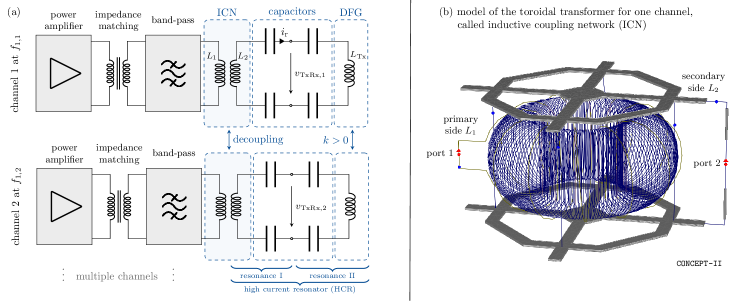
Figure 1: Overview of the MPI transmit chain and the ICN. In (a), the power amplifier is connected to a ferrite-core transformer, a band-pass filter and to the primary side of the ICN. The secondary side of this transformer is part of a high-Q resonator, called high current resonator (HCR), that includes the drive-field generator (DFG). Magnetic particles excited by the DFG induce signals via $L_{\textup{Tx}}$ and the receive signal is tapped within the symmetric HCR at $v_{\textup{TxRx}}$. In (b), a 4-fold segmented toroidal, D-shaped ICN is shown within a simulation setup of CONCEPT-II Institut für Theoretische Elektrotechnik (2023).

Our purpose of the resonant transformer, referred to as inductive coupling network (ICN), is to obtain a differential voltage system and a safe operating voltage. Ground loops and long, high-current cables can introduce undesired harmonics or disturbances into the receive spectrum, i.e., induced by eddy currents in nonlinear components such as unsoldered joints (screws). These distortions can dominate important particle harmonics or sidebands that are essential to the imaging process. A differential design avoids a global ground node and is less susceptible to interference and noise. Another strong advantage of a differential setup are floating signals with respect to a patient under examination, who is always capacitively coupled to ground. A single-ended transmit chain entails the danger for humans if they come into contact with any single point in the system. As MPI systems strive for human trials Thieben et al. (2023); Vogel et al. (2023); Schmale et al. (2013); Borgert et al. (2013), this safety aspect can not be ignored. Furthermore, reducing voltage levels in proximity to the patient requires a low inductance DFG, which in turn requires large currents to maintain the same field specifications Schmale et al. (2015b); Thieben et al. (2023).

In this work, we design and implement a resonant toroidal inductive coupling network that encompasses concerns regarding safety and incorporates a strictly linear and loss-optimized design. We elaborate on our design decisions and weigh different conditions and restrictions to present a new approach of finding suitable parameter choices, i.e., for inductors, cross-section shape, parallel segments, gain and dimensions. Our reasoning is intended to be transferable to other transformers under similar constraints using resonant loads for applications beyond medical imaging. Further, we consider crosstalk by channel decoupling between multiple drive-field channels that each use an individual ICN and review multiple decoupling strategies. Based on a TxRx topology that was presented without details by Sattel et al. Sattel et al. (2015), this study elaborates on the original implementation and optimization of an ICN and tailors the design parameters to a human-sized head scanner Thieben et al. (2023).

II Motivation and Purpose

Many current MPI systems use dedicated receive coils, often in a gradiometer configuration Graeser et al. (2013, 2017), effectively suppressing feedthrough harmonics, interference and systemic background Paysen et al. (2018, 2020). However, receive coils take up valuable space and ultimately increase power consumption when signal generating coils have to be placed farther away, independent the method of feedthrough suppression Borgert et al. (2013). For preclinical systems with rodent-sized bores, power consumption can be managed, however, on the path to human-sized systems, this issue becomes a major challenge Schmale et al. (2015b); Borgert et al. (2013). The advantage of choosing to combine the transmit and receive circuitry is that it reduces system complexity and overall space requirements by eliminating the need for a dedicated receive coil nested within the DFG and the receive band-stop filter Weizenecker et al. (2009). One possible topology of a transmit-receive (TxRx) circuit is a symmetric HCR as shown in FIG. 1 (a) with a linear ICN, shown in FIG. 1 (b). The development of the ICN is driven by various design goals, including a. achieving floating potentials, b. ensuring linearity, c. attaining high current gain and high $Q$, d. designing circuit symmetry for excitation, filtering and signal reception, and e. modularizing for impedance matching.

Floating potentials

The first design goal concerns patient safety and avoids ground loops that may negatively affect signal reception. A galvanically isolated high current resonator (HCR) with an overall low voltage and floating potentials is achieved by many common transformer topologies. Floating potentials become relevant for a patient being examined in the scanner. Following the principle of the first fault case, the potential separation ensures that a patient is not exposed to a life-threatening current through single contact with the circuit. This would require contact at two separate points of the circuit, which drastically reduces the risk. For this unlikely event, we take the further precaution of reducing the overall voltage in the DFG and HCR by selecting low-inductance components Thieben et al. (2023); Ozaslan et al. (2020).

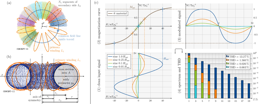
Figure 2: Segmented toroidal air-core transformer and THD simulation of iron-core saturation without hysteresis. Shown in (a) is a toroid parallelized with $N_{s}=12$ individual segments, of which $8$ are shown in different colors ($4$ are hidden). The primary winding also forms a toroid, here with $N_{1}=12$ turns, whereas each secondary segment has $N_{2}=13$ turns. In (b), the circular cross-section in the $xz$-plane is shown with characteristic parameters noted. On the right in (c), three sinusoidal input signals (1) are modulated by the magnetization curve in (2), which results in the output in (3) and its spectrum in (4). The magnetization curve is adopted from the “-8” iron powder core material Micrometals (2007), but without hysteresis effects and modeled with a $\tanh$-function Herceg, Chwastek, and Herceg (2020). A THD of $0.5\text{\,}\%$, typical for class-AB amplifiers, is caused by an amplitude of about $0.14\text{\,}$ of $H_{\textup{sat}}$.

Linearity

A strictly linear air-core transformer is required, because the ICN is located after the band-pass filter stage and must not increase the total harmonic distortion (THD) of the transmit or the receive signal. Harmonics generated directly within the HCR, where the receive signal is tapped, would be unfiltered and thus mask and alter the particle’s response. Harmonic generation by iron-core transformers is well known, due to core saturation effects Daut et al. (2010); Ramírez-Niño et al. (2016) and the principle is demonstrated in FIG. 2 (c). Here, we compare the THD after the band-pass filter with the THD generated by an ferrite-core transformer. Although an iron core would be preferable for its high permeability, effectively bundling magnetic field lines to achieve a high coupling coefficient $k$ and low leakage inductance, it introduces distortion due to saturation effects of the ferrite-core material. This constraint is so strong, that a THD of $0.5$ % from a class-AB power amplifier in combination with our transmit filter results in a theoretical THD benchmark of below $5\cdot 10^{-6}$ %, calculated using the fundamental definition THD${}_{\textup{F}}$  Shmilovitz (2005). The typical THD of linear power amplifier ranges from $0.1\,\%$ to $1\,\%$ AETechron (2023a, b); Crown (2023); Dr.Hubert (2023) and our filter achieves a measured $65$ dB amplitude attenuation at the second harmonic $f_{2}$, $100$ dB at $f_{3}$ and below $150$ dB at $f_{4}$ and above Mattingly et al. (2022); Thieben et al. (2023). Regarding a low-core loss iron powder material like “-8” (Micrometals, Inc., CA, USA Micrometals (2007)) and neglecting any hysteresis effects, a maximum amplitude deflection of only $1\,\%$ of the saturation field strength $H_{\textup{sat}}$ results in a THD of $3\cdot 10^{-3}\,\%$, as shown in FIG. 2 (c) (4). Although this number is extremely low, it is about 3 orders of magnitude higher than the combined THD of the amplifier and band-pass filter. Likewise, an amplitude of about $0.14\cdot H_{\textup{sat}}$ would cause a THD of $0.5$ %, counteracting any achievements by the band-pass filter. Moreover, intermodulation of harmonics will occur that further degrades the THD of an iron-core transformer, which was not modeled here. Consequently, an air-core transformer is preferred to achieve maximum linearity and a toroidal shape is advantageous to enclose the majority of field lines within the toroid. This minimizes any coupling leakage flux, eddy current losses in surrounding shielding and reduces the susceptibility to external disturbances to avoid spurious harmonics.

High current gain and high $Q$

In order to maintain the same excitation field using low-inductance components, higher currents are required Thieben et al. (2023). We are focusing on minimal conduction losses and an overall loss-optimized transformer design. The ICN is a resonant transformer, shown in FIG. 1 (b), and the secondary side of the transformer is part of the HCR. Note that both voltage and current are amplified on the secondary side, unlike non-resonant transformers. However, amplification is due to resonance and a change in the turns ratio still changes voltage and current in opposite directions. A limiting factor of the gain is the structural size, because it limits the overall achievable $Q$ of the HCR.

Independent of the desired inductor values, the cross-sectional shape of the toroid is optimized to maximize the inductance $L_{2}$ for a given wire length, i.e. the perimeter $p_{0}$ of the toroidal cross-section (D-shape). To achieve this, we implement the results of a comprehensive study by Murgatroyd Murgatroyd (1982). Additionally, frequency dependent losses are minimized by using litz wires that suppress the skin effect and reduce proximity effect losses Sullivan (1999). Due to the angular symmetry of the toroid, the winding core offers the possibility of parallel segmentation of the secondary side. Such parallel segments share the same enclosed field lines to compose a single composite toroid as shown in FIG. 2 (a) and (b), which can be used to shift the desired value for $L_{2}$ at a constant $Q$ to change the desired turns ratio $n$. A trade-off must be made between wire diameter, feasible parallelization of toroidal segments, stacked wire layers near the symmetry axis, heat dissipation, and target inductance.

TxRx circuit symmetry

Symmetry refers to the HCR layout, where the capacitors are split into two separate banks for each inductor, as shown in FIG. 1 (a). This offers the advantage of combining transmit and receive chains in a single circuit, as proposed by Sattel et. al Sattel et al. (2015). Here, the HCR acts simultaneously as a filter for the fundamental frequency, allowing to tap the particle’s response $v_{\textup{TxRx}}$ during transmission. However, a partial attenuation of the particle signal is inevitable using this configuration because the strength of the particle signal relies on the proportion of inductors $L_{2}$ and $L_{\textup{Tx}}$, which we call the DFG matching condition.

Impedance Matching Modularization

For feasible impedance matching, a modularization into two matching stages is carried out, as shown in FIG. 1. The ICN can thus be designed without additional constraints regarding amplifier load matching, which is done separately by an amplifier matching stage. To this end, we use an ferrite-core transformer before the band-pass filter with a maximum amplitude below 10 % of $H_{\textup{sat}}$, as explained in paragraph b., on the condition that the transformer’s THD is similar to the amplifier’s THD and a band-pass filter is implemented afterwards.

III Theory

In this section, we present a systematic optimization of an inductive coupling network, delineating the theory and criteria employed to derive the configurations for both sides of the toroidal transformer. Our approach commences with an examination of the transformer’s current gain $G$ in subsection III.1 and III.2. The focus then shifts to optimizing the toroidal geometry with the goal of minimizing losses and maximizing the inductance as described in subsection III.3. This optimization process encompasses cross-sectional shape, multiple winding layers, segmentation, and primary winding characteristics. In order to select an appropriate inductance value, we proceed to the inductance matching condition specific to a symmetric setup of the HCR in subsection III.4, a consideration tailored for the MPI imaging modality.

Given the broader context of multichannel MPI systems, it is imperative to devise individualized ICNs for each channel and account for coupling, which is described in subsection III.5. Nevertheless, up to that point, the entire section focuses on a single channel with the resonance frequency $f_{1}$.

III.1 Maximum Transformer Current Gain

The current amplification factor, denoted as $G$ for the ICN transformer, will be investigated with the objective to maximize it, according to design goal c. A first expression for $G$ can be derived by considering the power $P_{2}$ on the secondary side, caused by the primary current $i_{1}$ that induces the voltage $v_{2}$ as in

$$P_{2}=\frac{|v_{2}|^{2}}{R_{\textup{s}}}=\frac{|j\omega Mi_{1}|^{2}}{R_{\textup{s}}}=\frac{\omega^{2}M^{2}|i_{1}|^{2}}{R_{\textup{s}}}\;,$$ (1)

where $\omega=2\pi f_{1}$ denotes the channel angular frequency, $j$ the imaginary unit, $M$ the mutual inductance of the transformer, and $R_{\textup{s}}=R_{2}+R_{\textup{Tx}}$ the total series resistance of the secondary side at resonance (capacitor losses are neglected) Mett, Sidabras, and Hyde (2016). All components, currents and voltages are shown in FIG. 3. Now, the power at resonance can be rewritten to obtain the current gain $G$ by

$$|i_{2}|^{2}R_{\textup{s}}=\frac{\omega^{2}M^{2}|i_{1}|^{2}}{R_{\textup{s}}}~{}~{}\Rightarrow~{}~{}G=\frac{i_{2}}{i_{1}}=\frac{\omega M}{R_{\textup{s}}}\;.$$ (2)

In the following, this expression is rearranged for resonant transformers, using characteristic transformer variables like the turns ratio $n$, the coupling coefficient $k\in[0,1]$, and the quality factor $Q$ of the transformers secondary side Ayachit and Kazimierczuk (2016); Witulski (1995). Note that voltages across the leakage inductance $L_{\sigma,1}=L_{1}(1-k)$ and matching capacitor $C_{\textup{m}}$ of the band-pass filter cancel at resonance. Further, $L_{2}$ is part of a resonant circuit on the secondary side, therefore voltage and current are increased.

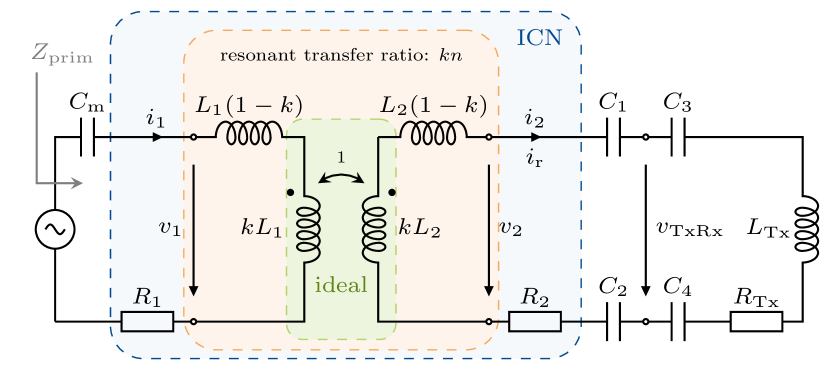
Figure 3: Resonant transformer circuit diagram. A resonant transformer is shown, where an ideal transformer remains embedded in the center. The inductors are split into leakage and coupled inductances. The matching capacitor $C_{\textup{m}}$ resembles the filter output stage, which goes into resonance with the leakage inductance $L_{\sigma,1}=L_{1}(1-k)$ and $Z_{\textup{prim}}$ becomes real at $\omega=2\pi f_{1}$.

The turns ratio is defined by the number of primary turns $N_{1}$ to secondary turns $N_{2}$. For an ideal transformer that is perfectly coupled ($k=1$), there is no phase difference and therefore no losses between the two sides. In this case, $n$ directly relates the magnitude of the voltages $v_{1}$ and $v_{2}$ and can be used to step up or step down the reflected impedance seen at the input Witulski (1995), as given in

$$n=\dfrac{N_{1}}{N_{2}}=\sqrt{\dfrac{L_{1}}{L_{2}}}=\frac{v_{1}}{v_{2}}\;.$$ (3)

$L_{1}$ and $L_{2}$ are the transformers primary and secondary inductances. Next, to obtain the coupling coefficient, we first regard the coupling factors

$$K_{1}=\frac{\Phi_{21}}{\Phi_{11}}=\frac{M}{L_{1}}\;,\;\;\;K_{2}=\frac{\Phi_{12}}{\Phi_{22}}=\frac{M}{L_{2}}$$ (4)

for the general case of arbitrary transformer shapes. $K_{1}$ measures the proportion of the mutual magnetic flux $\Phi_{21}$ caused by a current $i_{1}$ in $M$ and the magnetic flux $\Phi_{11}$ caused by a current $i_{1}$ in $L_{1}$. The same principle applies to $K_{2}$. Note that the values of $K_{\textup{i}}$ can be greater than 1. The mutual inductance $M$ is reciprocal for all linear materials with symmetric tensors for electric conductivity, permittivity and permeability Zacharias (2022). Now, the definition of the coupling coefficient is given with

$$k=\dfrac{M}{\sqrt{L_{1}L_{2}}}=\sqrt{K_{1}K_{2}}\;\;.$$ (5)

Lastly, a general expression for the quality factor $Q$ is given by the ratio of stored energy to dissipated energy per cycle: For an inductor $L$, perfect capacitors, and assuming negligible radiation losses in the $\mathrm{kHz}$ region, the quality factor is

$$Q=2\pi\frac{E_{\textup{stored}}}{\frac{1}{f}P_{\textup{diss}}}=2\pi f\,\frac{\displaystyle\int_{0}^{\hat{i}}L\;i\,\textrm{d}i}{\left(\frac{\hat{i}}{\sqrt{2}}\right)^{2}R}=\frac{\omega L}{R}\,.$$ (6)

$R$ is the total resistance of the considered resonance Zolfaghari, Chan, and Razavi (2001) and $\hat{i}$ the total current of the inductor.

Under the consideration of a dominant $Q$ of the coils, the three constituents of the gain in (2) are replaced for the considered ICN and the equation yields

$$G=\frac{\omega M}{R_{\textup{s}}}=\frac{\omega L_{2}}{R_{\textup{s}}}\,\dfrac{M}{\sqrt{L_{1}L_{2}}}\,\sqrt{\dfrac{L_{1}}{L_{2}}}=Q\,k\,n\,.$$ (7)

Note, that the inserted $Q$ refers to the transformer with its energy stores $L_{2}$, $C_{1}$, and $C_{2}$, while the resonance on the right side acts like a real impedance, adding only the serial resistance $R_{\textup{Tx}}$ of the DFG.

There are three conclusions due to (7): The channel frequency should be chosen as high as reasonable, taking into account the drawback of increasing losses due to high-frequency effects in the transmit and receive chains. We consider fixed frequencies in the low $\mathrm{kHz}$ range (around $26\text{\,}\mathrm{kHz}$) and discuss the frequency choice in section VI. Second, a reduction of $R_{\textup{s}}$ is beneficial: The correct type of litz wire should be chosen Sullivan (1999), connections within the HCR should be kept short, and the cross-section shape of the inductor should be chosen to obtain a minimum $R$ for maximum $L$ Murgatroyd (1982, 1989) to result in a high $Q$. Apart from minimizing $R$, the goal of maximizing $M$ requires finding a toroid with both, high $k$ and large $L$. A high turns ratio $n$ can be obtained by a dense primary winding and parallelizing the second transformer side. Third, as the total energy dissipated must equal the energy delivered in the resonant circuit we obtain

$$|P_{1}|\Delta t=|P_{2}|\Delta t~{}~{}\Rightarrow~{}~{}\text{Re}(Z_{1})=G^{2}\,\text{Re}(Z_{2})\;,$$ (8)

for a time interval $\Delta t$ at steady-state, $Z_{1}=v_{1}/i_{1}$ and $Z_{2}=v_{2}/i_{2}$. The imaginary parts is zero at resonance and the real impedance seen by the primary side equals

$$\text{Re}(Z_{\textup{prim}})=R_{1}+G^{2}\,R_{\textup{s}}=R_{1}+\frac{\omega^{2}M^{2}}{R_{\textup{s}}}\;.$$ (9)

III.2 Structural Size Limits Q

As argued above, and evident from Eqs. 7, we need a large secondary inductance to obtain a high transformer gain. A large structural size is beneficial, because an increasing cross section $A$ increases the inductance faster than its reduction by the growing center radius $r_{\textup{c}}$, as approximated by the equation for a single-layer air-core toroid with a circular cross-section

$$L_{\textup{toroid}} \approx\frac{\mu_{0}N^{2}A}{2\pi r_{\textup{c}}}\;.$$ (10)

Here, $\mu_{0}$ is the vacuum permeability and dimensions are shown in FIG. 2 (b). However, a constant number of turns that is stretched around a growing cross-section will reach a point where the changes in inductance and resistance compensate. This problem and its parameter dependencies is a well known optimization problem, treated by Murgatroyd Murgatroyd (1982, 1989), and an overview can be found in Murgatroyd and Belahrache (1985). $A$ can be increased until an optimum is reached where the inductance is maximum for a given total wire length $l=N\,2\pi r$ of all turns. This is a restraint on $A$, and there exists an optimum for the ratio of outer to inner radius for a finite $l$. The optimum number of turns for toroids with a circular cross-section and wire diameter $d$ lies at $N=0.8165\sqrt{l/d}$ and in turn yields the ratio $r/r_{\textup{i}}=(0.8165)^{-2}\approx 1.5$ and the optimal inductance

$$L_{\textup{toroid,opt,circ}}\approx\frac{\mu_{0}\,d}{2\pi}\left(0.2722\left(\frac{l}{d}\right)^{\frac{3}{2}}+0.25\frac{l}{d}\right)\;,$$ (11)

as derived by Murgatroyd Murgatroyd and Belahrache (1985).

Optimal benefits are obtained from the correct area to radius ratio in combination with a large overall construction volume, coupled with a judicious selection of layers within the interior, as shown in FIG. 4 (b), and explained in subsubsection III.3.2. The upper limit is reached if the interior space is fully occupied by wires, which also affects the cross-section shape that deviates from a circle for outer layers Murgatroyd (1989); Murgatroyd and Eastaugh (2000). Overall, increasing the dimensions of the toroid leads to an increase in $L_{2}$, $Q$, and thus $G$. The maximum $Q$ is defined by the available construction volume.

III.3 Toroidal Transformer

The ICN toroid is optimized for a finite available construction volume: optimizing the cross-sectional shape for a higher inductance, taking into account multiple layers of winding and improving coupling of the primary winding. Then, segmentation provides a tuning mechanism that allows to change the nominal inductance with a constant inductance to resistance ratio Evans and Heffernan (1990) to a desired value.

III.3.1 Optimal cross-section: D-shape

A circular cross-section gives the largest area $A$ for a fixed turn perimeter $p_{0}$, but it does not provide the highest inductance for this wire length. This discrepancy is caused by the non-uniform flux density within $A$, which is denser towards the inside for toroids Shafranov (1973); Murgatroyd and Belahrache (1985), as shown in FIG. 4 (a). Due to the straight inner edge of the D-shape, it encompasses the higher magnetic flux density towards the $z$-axis of symmetry and yields approximately 15% more inductance than the circular window for the same $p_{0}$ Murgatroyd and Belahrache (1985).

For the single-layer DC loss optimized D-shape, the optimum was found to be

$$L_{\textup{toroid,opt,D}}\approx\frac{\mu_{0}\,d}{2\pi}\left(0.314\left(\frac{l}{d}\right)^{\frac{3}{2}}+0.25\frac{l}{d}\right)\;,$$ (12)

for $\frac{r_{\textup{o}}}{r_{\textup{i}}}=5.3$ and $N=0.565\sqrt{\frac{l}{d}}$ Murgatroyd (1989), as shown in FIG. 4 (a). The slope (orange) is obtained by a stepwise evaluation along the radial direction, given by

$$\frac{\text{d}z}{\text{d}r}=\pm\dfrac{\ln{\dfrac{\sqrt{r_{\textup{i}}r_{\textup{o}}}}{r}}}{\sqrt{\ln{\dfrac{r}{r_{\textup{i}}}}\ln{\dfrac{r_{\textup{o}}}{r}}}}\;.$$ (13)

Integrating the slope $\text{d}z/\text{d}r$ yields coordinates for the optimized quarter section shapes.

AC losses are mainly eddy current losses due to proximity effects, since the skin effect plays only a minor role in litz wire windings. The impact by the proximity effect is twofold, internal magnetic fields due to neighboring currents cause eddy currents, but they are dominated by the second effect due to the main toroidal field through the rest of the coil, acting on the entire litz wire bundle Sullivan (1999). Overall, this results in eddy currents causing local non-uniform current densities that require a more complex shape optimization for high frequencies, that can be found in Murgatroyd (1982). The optimum shape for high frequencies differs from a D-shape due to the stronger constraint of eddy current losses, which are highest near the center, causing the highest point of the slope to move outward. However, in the $\mathrm{kHz}$ range, the AC optimized shape converges to the DC optimized shape of (13) for litz wires with sufficiently small strands.

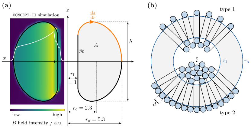
Figure 4: Optimal D-shaped cross-section and multilayer toroids Murgatroyd (1989). In (a), the optimal D-shape cross-section is shown for the fixed optimum ratio of ${r_{\textup{o}}}/{r_{\textup{i}}}=5.3$. The left toroid-half features a field intensity plot with the field profile along the $x$-axis in white (the toroid has 3 layers on the inside, simulated in CONCEPT-II Institut für Theoretische Elektrotechnik (2023)). Highlighted in orange in the right toroid-half is the curve obtained by a stepwise evaluation and integration of (13). In (b), two different types of winding arrangements of multi-layer toroidal inductors are shown.

III.3.2 Multiple Layers

Another way to effectively increase $L_{2}$, which optimizes $Q$, is by using multiple wire layers. However, insufficient heat dissipation from inner layers becomes an issue that in turn increases copper resistance and might damage the litz wire insulation layer. To this end, we propose a single nearly dense outer layer of turns as shown in FIG. 4 (b), which overlap on the inside near the axis of symmetry. This compromise gives satisfactory results and sufficient heat dissipation by air cooling. If the litz wire winding is not operated near their maximum current rating, e.g. for split-core toroids in filter stages Thieben et al. (2023); Mattingly et al. (2022), multiple dense layers are an efficient option. A general study on optimal shapes for air cores and non-air core multilayered toroidal inductors can be found in Murgatroyd and Eastaugh (2000).

III.3.3 Segmentation

The secondary side $L_{2}$ can be divided into $N_{\textup{s}}$ identical segments, which are wired in parallel but enclose a single common field, as shown in FIG. 2 (a) and (b). If the winding remains otherwise unchanged, both the inductance and the resistance will be reduced with $N_{\textup{s}}^{2}$, if $N_{\textup{s}}$ is increased. As an example, a segmentation into two halves is considered, where one half is limited to ${N}/{N_{s}}={N}/{2}$ turns. Intuitively, it seems that $L$ is reduced quadratically and the resistance $R$ reduced linearly, for a dense winding that remains unchanged, due to $L\sim N^{2}$ via (10) and $R\sim N$ via each turn perimeter. However, the effect for $L$ is changed to $L\sim N$ due to the shorter magnetic core length $l$, exemplified by a solenoid with $L\sim N^{2}/l\sim N$. An additional slight decrease is caused by the now open magnetic circuit, which results in less coupling of the end turns with the rest of the toroid. Mutual coupling $M$ compensates for this loss of self-inductance $L$ for toroids, since the halves now couple to the parallelized second half, i.e. to their neighbors at both ends. However, parallelizing equal impedances results in a $1/N_{\textup{s}}$ division for both $L$ and $R$. Overall, the linear contribution of the separation and the linear contribution of the parallelization result in a $1/N_{\textup{s}}^{2}$ scaling for both $L$ and $R$.

A segmented toroid with $N_{\textup{s}}=12$ segments is shown in FIG. 2 (a) and the total current is distributed by a central node (copper plates) at the top and bottom. A lead wire of each segment is connected to the node as shown in FIG. 1 (b) for $N_{\textup{s}}=4$. Another aspect of the segmentation is that the current $i_{\textup{r}}$ of the HCR is divided equally among the parallel segments, thus relaxing the copper cross section requirements for the $L_{2}$ winding. In system design situations, the construction volume is usually constrained to a maximum bounding box. For an optimal shape, $Q$ is thus fixed. Using this method, the design can start with an optimal single winding inductor and then use the segmentation to tune for a desired $L_{2}$ and $R_{2}$.

III.3.4 Primary Winding

A final design decision of the toroidal topology concerns the primary winding. For a reasonable volume and therefore limited $Q$, the primary winding should achieve a high coupling $k$, as seen in (7). Consequently, one choice is that $L_{1}$ is also toroidal and (sparsely) wound around the outside of $L_{2}$. This ensures that the majority of the field lines are shared by both transformer sides, to maximize $k$. In FIG. 2 (b), such a toroidal primary winding of $L_{1}$ (orange) is shown for a toroid with a circular cross-section. Known from Rogowski coils Rogowski and Steinhaus (1912) is the beneficial effect of a return wire in the $xy$-plane that counteracts the single turn of $l$ along the center circumference of the toroid to diminish the field on the outside, which is in line with the $z$-axis. For ease of fabrication, we propose a return wire along the outside at $r_{\textup{o}}$, which suppresses most of the stray field, but deviates from the optimal enclosed position at $r_{\textup{c}}$.

If a dense $L_{1}$ coil is used, i.e. a few turns at one point around the toroid, the result is a large $K_{1}$ and a very weak $K_{2}$. The overall $k$ is small, which is only sufficient for a design with a very large $Q$. However, such a dense $L_{1}$ provides several advantages for peripheral measures, like a pick-up coil to measure the current $i_{\textup{r}}$. Such a coil $L_{3}$ could be mounted on the toroid opposite to $L_{1}$ to focus its sensitivity locally to $L_{2}$ and avoid coupling between $L_{1}$ and $L_{3}$.

III.4 DFG Matching Condition

We have previously shown that, in order to achieve high gain for design goal c., it is advantageous to obtain a high $Q$. Currently, the inductance $L_{2}$ itself was not considered. In the following, a trade-off is identified that characterizes $L_{2}$ in dependence of $L_{\textup{Tx}}$ to comply with design goal d). This consideration arises from the specific constraints imposed by the MPI imaging setup, in particular the circuit symmetry condition for simultaneous transmission and reception, and the absolute power consumption, which has not been considered so far. Here, we assume a constant $Q$, which is justified for a fixed bounding box as reasoned in subsection III.2, resulting in a linear relationship of $R_{2}$ and $L_{2}$ at a fixed $\omega$. The ohmic resistances of the capacitors and the DFG remain constant.

Our objectives are twofold, yet inherently contradictory: achieving both maximal particle signal strength at the $v_{\textup{TxRx}}$ port and minimal power consumption within the HCR. The particle response is characterized by the prevalence of high-order harmonics of the resonance frequency $f_{1}$. These harmonics experience a significant voltage drop across an inductive voltage divider formed by the inductances $L_{2}$ and $L_{\textup{Tx}}$ when compared to the relatively minor influences of their small series resistances within the $\mathrm{m\SIUnitSymbolOhm}$ range Thieben et al. (2023) and the associated HCR capacitors at harmonic frequencies. The winding configuration of $L_{\textup{Tx}}$ can be conceptualized as a distributed voltage source, thereby inducing the particle voltage at the virtual ground nodes of $v_{\textup{TxRx}}$ Sattel et al. (2015). Ideally, in the scenario of an infinitely large $L_{2}$, the complete induced voltage would be dropped across $L_{2}$, leading to a maximal particle response at $v_{\textup{TxRx}}$. In contrast, a diminished ratio of $L_{2}/L_{\textup{Tx}}$ would effectively short-circuit the receive voltage, advocating a maximum value for $L_{2}$. However, the cumulative series resistance $R_{2}\sim N\,2\pi r$ of the toroid manifests the same increase as $L_{2}$ is augmented, as imposed by a constant $Q$ via (6). The total power consumption increases with $R_{2}$, but it is limited to a feasible amount. This imposes a constraint on $L_{2}$, because the current amplitude at resonance $i_{\textup{r}}$ in the HCR must stay constant to maintain the same drive field strength. Consequently, a partial attenuation of the particle signal is inevitable due to the voltage division effect inherent in the inductance voltage divider of $L_{2}$ and $L_{\textup{Tx}}$.

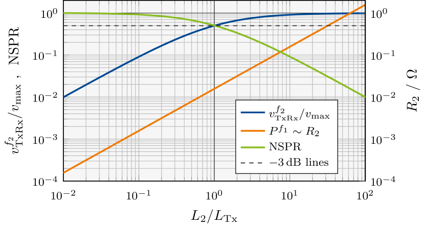
Figure 5: Inductance matching condition of DFG and ICN. A trade-off is identified at $L_{2}=L_{\textup{Tx}}$, when the receive signal is halved ($-3\text{\,}\mathrm{d}\mathrm{B}$), expressed by the intersection of the particle signal (blue) and the normalized signal-to-loss ratio (green). This graph demonstrates that additional power is required to avoid receive signal attenuation.

The crucial point is that the power consumption at the fundamental $f_{1}$ scales linearly with $R_{2}$ and the particle voltage at frequencies $f>f_{1}$ drops depending on the inductive voltage divider, when the impedance of capacitors becomes negligible. We consider a unit current $i_{\textup{r}}=$1\text{\,}\mathrm{A}$$ and define the particle signal-to-power ratio (SPR) as

$$\text{SPR}=\frac{v_{\textup{TxRx}}^{f_{2}}}{P^{f_{1}}}=\frac{v_{\textup{TxRx}}^{f_{2}}}{i_{\textup{r}}^{2}\,R_{2}}\,.$$ (14)

The power consumption $P^{f_{1}}$ is considered at the fundamental, but the particle signal $v_{\textup{TxRx}}^{f_{2}}$ at the first harmonic. Note that for $f_{2}$ and all higher frequencies the inductive voltage divider is the dominant part and all harmonics are recorded. The maximum particle voltage $v_{\textup{max}}$ of $v_{\textup{TxRx}}^{f_{2}}$ is defined in the limit of a large $L_{2}$, where it is not attenuated. To remove the influence of the absolute value of $R_{2}$, we normalize (14) with its maximum in the parameter range and call it NSPR. The constituents of (14) and the NSPR are plotted in FIG. 5.

One possible trade-off position can be identified at $-3\text{\,}\mathrm{dB}$ of NSPR and $v_{\textup{TxRx}}^{f_{2}}$, that results in halving the receive signal (harmonics). This point coincides with $L_{2}=L_{\textup{Tx}}$, where the inductances match, which we chose as the trade-off for the design of our ICNs. Consequently, a less attenuated particle signal requires more power. Note that (14) remains valid when $L_{\textup{Tx}}$ is varied instead of $L_{2}$ and the consideration of the inductance voltage divider remains identical.

III.5 Channel Decoupling

The use of multiple channels in MPI has the advantage of simultaneous sampling of a 3D field-of-view (FOV). Due to imperfect spatial orthogonality of these channels and close proximity of resonance frequencies, typically within a range of less than $\Delta f=0.03f_{1}$ Knopp, Gdaniec, and Möddel (2017), strong coupling between the different drive-field channels is expected. Thus even weak coupling coefficients presents a particular challenge, especially in case of resonant circuits with high $Q$, necessitating the development of effective decoupling mechanisms with introducing minimal additional resistance to the HCR.

Causes of channel coupling are misalignment of the drive-field coils, non-orthogonal field components, and undesired loops in the connecting wires. Small errors in positioning, e.g. for two planar coils with $k\sim\cos(\beta)$, can lead to coupling with significant currents. A $\beta=$3\text{\,}\mathrm{\SIUnitSymbolDegree}$$ results in $k=0.052$, which can generate a current $i_{\textup{r,2}}$ in channel 2 of similar magnitude to the original current $i_{\textup{r,1}}$ in channel 1. For this purpose, if we consider the complex impedance $Z_{\textup{HCR,2}}$ of the second channel’s HCR and let $j$ be the imaginary unit, then the current $i_{\textup{r,2}}$ in the second channel at the first angular frequency $\omega_{\textup{r,1}}$ is caused by induction via $i_{\textup{r,1}}$ and $M$, as in

$$\frac{i_{\textup{r,2}}(\omega_{\textup{r,1}})}{i_{\textup{r,1}}(\omega_{\textup{r,1}})} =\frac{v_{\textup{ind,21}}(\omega_{\textup{r,1}})}{Z_{\textup{HCR,2}}(\omega_{\textup{r,1}})}\frac{1}{i_{\textup{r,1}}(\omega_{\textup{r,1}})}$$

$$=\frac{j\omega_{\textup{r,1}}M\,i_{\textup{r,1}}(\omega_{\textup{r,1}})}{Z_{\textup{HCR,2}}(\Delta\omega+\omega_{\textup{r,2}})\,i_{\textup{r,1}}(\omega_{\textup{r,1}})}$$ (15)

$$\approx\frac{j\omega_{\textup{r,1}}M}{j2\Delta\omega(L_{\textup{Tx,2}}+L_{\textup{2,2}})}\approx\frac{\omega_{\textup{r,1}}M}{4\Delta\omega L_{\textup{2,2}}}=\frac{1}{4}\frac{\omega_{\textup{r,1}}}{\Delta\omega}\,k\,.$$

Note that the matching criterion of subsection III.4 is respected with $L_{\textup{Tx,2}}=L_{\textup{2,2}}$ and we approximate $Z_{\textup{HCR,2}}$ near $\omega_{\textup{r,2}}$ with $j2\Delta\omega L_{2,2}$ as shown in the appendix A.1. With $\tfrac{\Delta\omega}{\omega_{\textup{r,1}}}=\tfrac{(\omega_{\textup{r,1}}-\omega_{\textup{r,2}})}{\omega_{\textup{r,1}}}=\tfrac{1}{75}$ (see beginning of section V) and the aforementioned misalignment of $\beta=$3\text{\,}\mathrm{\SIUnitSymbolDegree}$$, this example results in $\tfrac{i_{\textup{r,2}}}{i_{\textup{r,1}}}=0.25\cdot 75\cdot 0.052=0.975\approx 1$. The consequence is a severe distortion of the Lissajous trajectory, which is already significant for values ${i_{\textup{r,2}}}/{i_{\textup{r,1}}}\geq$10\text{\,}\%$$ von Gladiss, Graeser, and Buzug (2018).

In order to avoid the negative effects of uncompensated coupling, such as trajectory distortion, additional power dissipation, detuning, and frequency beating that will act on the power amplifier, we consider 3 types of decoupling schemes: capacitive, inductive and active compensation. Capacitive compensation is narrowband and requires additional connections between channels, but the equivalent series resistance (ESR) of capacitors is low. Inductive compensation is directed at counteracting $M$ and is broad-band, but additional coils typically increase the series resistance, thus reducing $Q$. Finally, active decoupling uses the channel’s amplifiers, but demands reactive power in the band-pass filters (FIG. 1 (a)) and for the miss-matched HCR. Further, it requires accurate feedback for current control. It should be considered a last resort, as the amplifier will see a reactive load at other frequencies, and maximum voltage ratings may be exceeded over the course of a full Lissajous trajectory cycle.

In general, capacitive decoupling may not offer an exact solution, and there are unsolvable combinations of coupling depending on the sign of the coupling coefficients. However, capacitive compensation is advantageous for the particle signal of a transmit-receive circuit because a large common series capacitor can be used, which becomes a short at harmonic frequencies and has a very low series resistance compared to coil windings. This requires two common nodes between channels and similar inductive coupling coefficients of the same sign, due to the single narrowband decoupling point. We could use 3 capacitors, 2 within each channel or alternatively one common capacitor for all channels. The mentioned low differences of drive-field frequencies in MPI are a premise, and a limitation is that the sum of all currents flows through this capacitor. A schematic is shown in FIG. 6 (a), which represents only the right part of the symmetric HCR, with $v_{\textup{TxRx}}$ across each numbered a-b terminal pair, shown for 3 channels each.

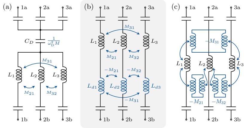
Figure 6: Schematic of decoupling schemes with 3 TxRx channels. The schematics refer to one half of the symmetric HCR, where $v_{\textup{TxRx}}$ can be tapped across each numbered a-b terminal pair (compare FIG. 1). Capacitive decoupling for a single frequency via a common capacitor $C_{\textup{D}}$ is shown in (a), with the condition of $M_{21}\approx M_{32}\approx M_{31}$. Inductive decoupling strategies (broadband) are shown in (b) and (c), for the case of series inductors and the case of separate windings, respectively.

Inductive compensation is a general alternative for all coupling coefficient signs: Either a coil is added in series to $L_{\textup{Tx}}$ for each unique off-diagonal entry of the system’s impedance matrix as in FIG. 6 (b), or the same number of separate windings is used to introduce the desired compensation without a galvanic connection by careful positioning as shown in FIG. 6 (c). A disadvantage of the first technique is the additional high current lines, stray fields, their influence on the tuning of the resonators, additional series resistance, as well as their mounting and cooling effort. The second technique uses separate windings that are sensitive to a partial amount of the drive-field, equal to the $M$ introduced by coupling. A suitable inductive decoupling position is the ICN itself, as implied in the last paragraph of subsubsection III.3.4. Turns on the outer surface of the toroid are only capable of utilizing integer multiples to achieve a match with $M$. However, a slab outfitted with a wire loop can be introduced to encompass a partial quantity of the magnetic field inside: a loop on a slab that is inserted into a prepared gap within the toroid. Adjustment of the slabs can be used to fine-tune each channel if the ICN was prepared with such gaps. The sign can be adapted by inverting the orientation of the wire-loop. However, the principle remains the same if it is done with partial fields in the proximity of the DFG.

For our two-channel human-sized system Thieben et al. (2023), we decided to use a single common capacitor that carries a peak current of $i_{\textup{r,1}}+i_{\textup{r,2}}$ (depending on the phase of the Lissajous cycle), introducing the same voltage as $M$ into each circuit, but with opposite sign. The common decoupling capacitor $C_{\textup{D}}$ is calculated at a single frequency $\omega_{\textup{D}}$ in-between both drive-field frequencies by

$$C_{\textup{D}}=\frac{1}{\omega_{\textup{D}}^{2}M}=\frac{1}{(\pi(f_{\textup{r,2}}+f_{\textup{r,1}}))^{2}\;k\sqrt{L_{\textup{Tx,1}}L_{\textup{Tx,2}}}}$$ (16)

This narrowband solution is acceptable for our implemented two-channel system, and the additional ESR introduced by the decoupling capacitor is small.

IV Methods and Implementation

Guided by the theory to optimize the ICN for a given bounding box, we now describe the implementation and name the changes to our design that deviate from the stated optimum. We employ simulations to assess performance in subsection IV.1, which include a D-shaped toroid and are used to refine our decision on the number of segments and the type of primary winding. The construction of two ICNs is described in subsection IV.2 and the measurement methodology to analyse the prototypes is given in subsection IV.3.

IV.1 Simulations

Linear circuit simulations are performed with LTspice 17.1 (Analog Devices, MA, USA) Analog Devices Inc. (2023). Simulations of the magnetic field and the transformer’s impedance matrix are performed using CONCEPT-II (Institut für Theoretische Elektrotechnik, Hamburg University of Technology, Germany) Institut für Theoretische Elektrotechnik (2023).

IV.1.1 Toroid Geometry

The CONCEPT-II software is based on the method of moments (MoM) that solves electromagnetic boundary or volume integral equations in the frequency domain Gibson (2008). It is especially suited for the numerical computation of 3D radiation and scattering problems. CONCEPT-II is used in our work to calculate and test different toroidal transformer configurations. Input parameters include the general geometry (distances, shape and size of $A$, number of segments $N_{\textup{s}}$, turns $N_{1}$ and $N_{2}$, primary winding shape, number of overlapping layers inside the toroid), while important output parameters include the impedance matrix $\bm{Z}$, 3D field plots and conductors current densities. A two-port network is used to estimate $k$ and $G$ via the impedance matrix of the transformer

$$\bm{Z}=\begin{bmatrix}Z_{11}&Z_{12}\\ Z_{21}&Z_{22}\end{bmatrix}\approx\begin{bmatrix}R_{\textup{1}}+j\omega L_{1}&j\omega M\\ j\omega M&R_{\textup{2}}+j\omega L_{2}\end{bmatrix}\,.$$ (17)

Different numbers of segments $N_{\textup{s}}$ are simulated as well as the coupling between neighboring segments. Stray fields are minimized and coupling is maximized by looking at different winding options for $L_{1}$ (dense vs. sparse/distributed), the suited number of turns $N_{1}$, and the current density in the copper-plates where parallel segments are joined. Litz wire windings are approximated by a single thin wire, assuming that the currents are restricted to the direction of the wire, and copper conductivity of surfaces and wires is set to $\sigma=$58\text{⋅}{10}^{6}\text{\,}\mathrm{S}\text{\,}{\mathrm{m}}^{-1}$$. The results of the simulation are used to adapt the design and finally to compare the expectations with the manufactured prototypes in terms of $L$, $k$, $n$, and $G$. One simulated $B$-field plot is shown in FIG. 4 (a) for a number of 3 overlapping wire layers on the inside. One complete model (4 segments) is shown within the simulation framework in FIG. 1 (b), including copper distribution plates.

IV.1.2 Circuit Analysis

With simulated values for $L_{1}$, $L_{2}$, $k$ and resistors as input parameters, the resonance behavior is analyzed in the schematic circuit analyzer tool LTspice. A model of the entire HCR is simulated, including the band-pass filter stage, the ICN and two channels including crosstalk. Different decoupling strategies are tested to probe the schematic, based on FIG. 3, and to tune values for decoupling elements. The input impedance value $Z_{\textup{prim}}$ was also simulated with LTspice.

Table 1: Values from simulation (yellow) and measurement (blue) for both constructed ICNs. Bold font denotes important values.

			$L$ / $\mathrm{\SIUnitSymbolMicro H}$	$R$ / $\mathrm{m\SIUnitSymbolOhm}$	$N$	$f_{1}$ / $\mathrm{H}\mathrm{z}$	$M$ / $\mathrm{\SIUnitSymbolMicro H}$	$Q_{\textup{ICN}}$	$Q_{\textup{HCR}}$	$n$	$k$	$G$	$Z_{\textup{prim}}$ / $\mathrm{\SIUnitSymbolOhm}$	$L_{\textup{Tx}}$ / $\mathrm{\SIUnitSymbolMicro H}$	$R_{\textup{Tx}}$ / $\mathrm{m\SIUnitSymbolOhm}$
ICN 1	sim.	$pri.$	6.21	200	12	25699	5.47	219	90.1	0.62	0.54	30.2	26.8
		$sec.$	16.3	12.0	$4\cdot 36$
	meas.i	$pri.$	6.65	233	12	25699	6.08	215	90.8	0.63	0.57	33.0	32.6	14.4	17.2
		$sec.$	16.7	12.5	$4\cdot 36$
ICN 2	sim.	$pri.$	6.88	200	13	26042	4.09	230	77.1	0.94	0.56	40.8	27.6
		$sec.$	7.73	5.5	$6\cdot 24$
	meas.i	$pri.$	6.85	210	13	26042	4.39	220	76.4	0.94	0.60	43.0	31.1	9.74	10.9
		$sec.$	7.8	5.8	$6\cdot 24$

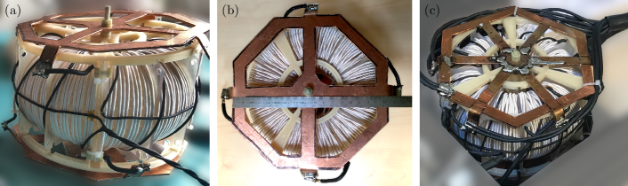
Figure 7: Two ICNs for a two channel MPI system. In (a), the ICN 1 with $N_{\textup{s}}=4$ segments is shown (primary winding in black) and in (b) the top of the same ICN is shown with a reference scale in cm (without primary winding). ICN 2 with $N_{\textup{s}}=6$ segments is shown in (c), after installation. The connecting litz wire of the HCR and the primary winding are insulated with black shrinking tube.

IV.2 Construction of two Toroidal ICNs

To weigh different design decisions of the ICN, we followed the reasoning of section III and IV.1 consecutively. The construction was performed after the simulation, with the probed values for parameters $L$, $N$, the number of segments $N_{\textup{s,1}}=4$ and $N_{\textup{s,2}}=6$ as given in TABLE 1, and the chosen dimensions of $r_{\textup{i}}=$4\text{\,}\mathrm{cm}$$, $r_{\textup{o}}=$9.2\text{\,}\mathrm{cm}$$, and the height $h=$8.6\text{\,}\mathrm{cm}$$ for the D-shaped second side. Moreover, we use the channel frequencies $f_{1,1}=$25.699\text{\,}\mathrm{kHz}$$ and $f_{1,2}=$26.042\text{\,}\mathrm{kHz}$$ with a distance of $\Delta f=$343\text{\,}\mathrm{Hz}$$.

The choice of $N_{\textup{s}}=6$ segments for the second channel is owed to the fact that we implemented a saddle coil (DFG of channel 2), which requires a higher current than the first channel to meet field specifications Thieben et al. (2023), thus we choose to reduce $R_{2}$. Due to the fact that $Q$ remains constant, the increase in gain is caused by the turns ratio $n$ due to the shift in the ratio of $L_{1}$ to $L_{2}$. As reasoned in subsubsection III.3.3, the inductance decreases for a higher number of segments, which also better fits to the lower DFG inductance of the saddle coil to comply with the matching condition of subsection III.4. To further increase the turns ratio $n$ of the second channel, we chose $N_{1,2}=13$ instead of $N_{1,1}=12$. As a consequence, we were able to use the same support structure for winding and both ICNs are of equal dimensions in spite of their different objectives. The 3D printed toroidal support structure of the ICN is made from the high temperature resin RS-F2-HTAM-02 (Formlabs, MA, USA). Air cooling along the symmetry axis is installed using shielded fans, to prevent impedance changes by insufficient heat dissipation.

A difference between the derived optimal design and the constructed ICNs is the ratio of radii $r_{\textup{i}}/r_{\textup{o}}=2.3$ for the D-shaped toroid. This deviation to the optimum of $r_{\textup{i}}/r_{\textup{o}}=5.3$ is a compromise to gain more space for a feasible winding through the center of the toroid, to reduce the amount of inner layers, to increase the air cooling surface, and to comply with a limit on the available construction height. Basically, we calculated the optimal design to fully utilize the available construction space height $h$, and then opted to increase $r_{\textup{i}}$ while keeping the other parameters constant.

Regarding the primary winding, a dense (localized) winding is unsuited due to a low $k$, as reasoned in subsubsection III.3.4. Sparse windings on a helical path yielded best results, thereby forming a toroid on top on the outer surface around the $L_{2}$ toroid, as shown in FIG. 2 (a), (b) and FIG. 7 (a).

To minimize AC losses within the conducting material, a silk-wrapped litz wire of $2000$ strands of $50\text{\,}\mathrm{\SIUnitSymbolMicro m}$ copper (effective copper cross-section of $3.1\text{\,}\mathrm{m}\mathrm{m}^{2}$) is used for the secondary transformer winding. The primary winding consists of $400$ strands of $50\text{\,}\mathrm{\SIUnitSymbolMicro m}$ copper (effective copper cross-section of $0.78\text{\,}\mathrm{m}\mathrm{m}^{2}$) and is wrapped in shrinking tube to increase durability and breakdown voltage. Parallel segments are connected on a $1\text{\,}\mathrm{mm}$ thick copper plate (top and bottom), which serves primarily as a distribution platform and to connect parallel litz wires of the HCR and the ICN with a solder connection. Also, balancing currents can be equalized on this low resistance copper plate.

IV.3 Measurements

Measurements of inductors are performed with the LCR meter Keysight E4980AL (Keysight Technologies, CA, USA) at the channel’s frequency. The coupling coefficient of a transformer is measured by using the short and open circuit inductances Hayes et al. (2003) in

$$k\approx\sqrt{1-\frac{L_{\textup{1,\,$L_{2}$\,short}}}{L_{\textup{1,\,$L_{2}$\,open}}}}\;.$$ (18)

Note, that $L_{2}$ needs to be sufficiently shorted (more difficult at high frequencies) and the quality factor of the secondary side should be $Q>50$ for this model to be accurate.

The LCR meter is used for TABLE 1 to determine $L$, the series resistance $R$, and $k$ in the measured rows. All other values in these rows are calculated: $M$ via (5), $Q_{\textup{ICN}}$ via (6) with $L$ and $R_{2}$ of the same row, likewise $Q_{\textup{HCR}}$ with $L$ and $R_{\textup{s}}=R_{2}+R_{\textup{Tx}}$, $n$ via (3) using the primary and secondary measured $L$, and $G$ via (7) for each row. For the simulated rows of TABLE 1, $L$ and $M$ were obtained from the simulation in CONCEPT-II, and $k$ was calculated via (5) here .

V Results

We have designed, simulated and fabricated two ICNs with $f_{r_{1}}=$25.699\text{\,}\mathrm{kHz}$$ ($N_{\textup{s}}=4$) and $f_{r_{2}}=$26.042\text{\,}\mathrm{kHz}$$ ($N_{\textup{s}}=6$) for a two channel human-sized MPI system and integrated both into our MPI scanner Thieben et al. (2023). The simulation and measurement results of the final design are summarized in TABLE 1 and details of the construction are described in subsection IV.2. Pictures of both constructed ICNs are shown in FIG. 7.

The deviation between measured and simulated inductances $L_{2}$ is below $2.5\text{\,}\%$ and below $1\text{\,}\%$ for the first and second ICN, respectively. The measured value for $k$ is about $57\text{\,}\%$ larger than the simulated value. Therefore $M$ is also larger in rows 2 and 4, because its calculation is based on $k$ and $L_{2}$. This results in the measured $G$ being $9.3\text{\,}\%$ and $5.4\text{\,}\%$ larger for ICN 1 and 2, respectively. $Q_{\textup{ICN}}$ refers only to the self-inductance $L_{2}$ and series $R_{2}$ of the secondary transformer side, while $Q_{\textup{HCR}}$ is the more important measure that includes the entire resonant load. Here, $R_{\textup{s}}=R_{2}+R_{\textup{Tx}}$ represent the losses of the HCR and resemble the gain actually achieved. Later current measurements showed a gain very similar to these values, although they are marginally lower due to losses of additional connections and wires (e.g. decoupling capacitor).

The inductors of DFG and ICN are nearly matched for both channels as explained in subsection III.4, with $L_{\textup{Tx,1}}=$14.4\text{\,}\mathrm{\SIUnitSymbolMicro H}$\approx L_{2,1}=$16.7\text{\,}\mathrm{\SIUnitSymbolMicro H}$$ for channel 1, and with $L_{\textup{Tx,2}}=$9.74\text{\,}\mathrm{\SIUnitSymbolMicro H}$\approx L_{2,2}=$7.8\text{\,}\mathrm{\SIUnitSymbolMicro H}$$ for channel 2. Note, that the target input impedance $Z_{\textup{prim}}$ of (9) remains for both ICNs at around $30\text{\,}\mathrm{\SIUnitSymbolOhm}$, which is the load after the band-pass filter. Also, $Q$ of both ICNs remains constant with $215\approx 220$ (measured values) for the different segmentation, as argued in subsection III.3. The increase in $G$ is achieved by augmentation of $n$ due to the segmentation.

Due to the non-orthogonal DFG channels, there is a residual coupling of $k=0.062$ Thieben et al. (2023), which has serious implications for both resonators, as described in subsection III.5. The channels were decoupled by $-35\text{\,}\mathrm{dB}$ using a single common decoupling capacitor carrying both currents $i_{\textup{r,1}}$ and $i_{\textup{r,2}}$. This choice provided good results with minimal changes to the existing HCR, without introducing a large series resistance and with high temperature stability.

VI Discussion

Applications that require highly linear transformers, such as MPI, rely on circuits that do not utilize magnetic materials that saturate. Any harmonic distortion may obscure the weak receive signal and degrade image quality. As a result, air-core structures are chosen at the expense of increasing component dimensions, which sets the maximum $Q$ for an available construction volume. In this study, we present a blueprint for a high-gain linear transformer with a high quality factor. We formulate an expression for the gain as a function of mutual inductance, optimize the cross-sectional shape, employ segmentation to shift the nominal inductance, deduce a primary winding topology, and incorporate multiple layers to enhance performance. In the context of the emerging imaging modality MPI, we establish a matching condition that balances particle signal and power consumption. Further, we elaborate on various decoupling techniques for multichannel systems and support our assessment of the ICN with simulations.

In terms of human safety, the entire HCR has floating potentials and component voltages in patient proximity are reduced by the ICN due to its high current gain that drives the low-inductance DFG to generate the required MPI drive-field. The symmetric design of the HCR allows for fundamental filtering at the signal tap, but results in partial receive signal attenuation due to the inductive voltage divider of $L_{2}$ and $L_{\textup{Tx}}$. The TxRx topology generally reduces power consumption by saving space through the elimination of dedicated receive coils, but consumption is approximately doubled by the ICN. In addition, common decoupling strategies such as gradiometric receive coils reduce the design requirements for linearity within the transmit chain. A direct comparison in signal quality between this TxRx topology and a gradiometric receive topology is currently pending, although other TxRx systems have been characterized Paysen et al. (2020).

The presented toroidal transformer blueprint is limited by its restriction to the quasi-static regime of electromagnetics, where wave propagation effects are not dominant. Additionally, if AC losses due to proximity effects dominate in the toroid, the D-shape optimization will result in a different shape Murgatroyd (1982). Parameters given or assumed in this study, such as frequency or volume, require careful selection: $Q$ increases linearly with frequency and should be chosen as high as possible, taking into account component voltages, high reactive power (in resonance) Schmale et al. (2015b), signal induction, wave propagation effects at high harmonics, required receive bandwidth, PNS and SAR limits Bohnert and Dössel (2010); Schmale et al. (2015a, 2013); Saritas et al. (2013); Grau-Ruiz et al. (2022). Our decision regarding the deviation of ${r_{\textup{o}}}/{r_{\textup{i}}}$ from the optimum was aimed at facilitating the winding process and reducing the number of stacked inner layers. This decision allowed winding a nearly dense outer layer with 2 to 3 stacked inner layers. Regarding (10) with a given constant area and a linearly increasing $r_{\textup{c}}$, we assume that the deviation from the optimal inductance is small. The copper plates at the top and bottom (nodes of parallel segments) should be designed to facilitate air cooling of the inner layers.

A key insight is that the available construction space should be exhausted and the quality factor of the ICN benefits from a large volume, yielding a high gain. Therefore, the construction volume should be as large as cost, weight, and size factors will allow. If a lower $L_{2}$ is desired compared to a single winding on the maximized toroid, segmentation provides the means to reduce both inductance and resistance at the same rate with a constant $Q$. Note, this also increases the turns ratio $n$, causing a higher gain $G$. Independent of geometric choices, the method of moment based simulation provided accurate results and the simulated inductance value deviated less than $2.5\text{\,}\mathrm{\char 37\relax}$ from the manufactured ICNs. Two linear ICNs were built based on our presented schematic optimization that feed a floating 2-channel HCR, including crosstalk decoupling, for a human-sized MPI head scanner Thieben et al. (2023) to fulfill safety precautions on a path towards the clinical integration of MPI.

Author Contributions

F.M. F.F., F.T., T.K., and M.G. contributed to the conceptualization and theory. F.M. and F.F. performed the simulations and measurements. F.M., F.F., F.T., and M.G. constructed the MPI components. I.S. contributed to the multi-channel circuit analysis and decoupling theory. T.K. and M.G. supervised the project. F.M. wrote the original draft with support of M.M., M.G., F.F., F.T., I.S. and T.K. All authors reviewed the manuscript.

Data Availability Statement

The data that support the findings of this study are available from the corresponding author upon reasonable request.

Appendix A Appendixes

A.1 Slightly Detuned Resonators

Let $\omega_{1}$ and $\omega_{2}$ be the channel frequencies of channel $1$ and $2$, respectively, and $\Delta\omega=\omega_{1}-\omega_{2}$. Only $\omega_{1}$ in channel $1$ is excited and we approximate the impedance of the coupled second resonator for small $\Delta\omega$. $R_{\textup{s,2}}$ is the real part of the resistance of channel $2$ at resonance. The first order Taylor series expansion of the impedance of channel $2$ yields

$$Z_{2}(\omega_{2}+\Delta\omega) =Z(\omega_{2})+\Delta\omega\cdot\left.\frac{\text{d}Z(\omega)}{\text{d}\omega}\right|_{\omega_{2}}$$

$$=R_{\textup{s,2}}+\Delta\omega\,j\left(L+\frac{1}{\omega_{2}^{2}C}\right)$$

$$=R_{\textup{s,2}}+j2\Delta\omega\,L\;.$$ (19)

We insert $L=\tfrac{1}{\omega_{2}^{2}C}$ which is an expression of the resonance condition $\text{Im}(Z_{2})=0$ at $\omega_{2}$ for a RLC resonant circuit. Here, $L$ is the sum of all inductances within the circuit. Consequently, we can rewrite (19) into

$$Z_{2}(\omega_{2}+\Delta\omega) =R_{\textup{s,2}}\left(1+j2\frac{\Delta\omega}{\omega_{2}}\frac{\omega_{2}L}{R_{\textup{s,2}}}\right)$$

$$=R_{\textup{s,2}}\left(1+j2\frac{\Delta\omega}{\omega_{2}}Q\right).$$ (20)

With a $\tfrac{\Delta\omega}{\omega_{2}}$ of $\tfrac{1}{75}$ and a $Q>200$, we obtain a dominating imaginary part and the equation simplifies to $Z_{2}(\omega_{2}+\Delta\omega)\approx j2\Delta\omega L$.

References

- Gleich and Weizenecker (2005) B. Gleich and J. Weizenecker, “Tomographic imaging using the nonlinear response of magnetic particles,” Nature 435, 1214–1217 (2005).
- Lauterbur (1973) P. C. Lauterbur, “Image Formation by Induced Local Interactions: Examples Employing Nuclear Magnetic Resonance,” Nature 242, 190–191 (1973).
- Schmale et al. (2015a) I. Schmale, B. Gleich, J. Rahmer, C. Bontus, J. Schmidt, and J. Borgert, “MPI Safety in the View of MRI Safety Standards,” IEEE Transactions on Magnetics 51, 1–4 (2015a).
- Dössel and Bohnert (2013) O. Dössel and J. Bohnert, “Safety considerations for magnetic fields of 10 mT to 100 mT amplitude in the frequency range of 10 kHz to 100 kHz for magnetic particle imaging,” Biomedizinische Technik/Biomedical Engineering 58 (2013), 10.1515/bmt-2013-0065.
- Gleich, Weizenecker, and Borgert (2008) B. Gleich, J. Weizenecker, and J. Borgert, “Experimental results on fast 2D-encoded magnetic particle imaging,” Physics in Medicine & Biology 53, N81—-N84 (2008).
- Schmale et al. (2013) I. Schmale, B. Gleich, J. Schmidt, J. Rahmer, C. Bontus, R. Eckart, B. David, M. Heinrich, O. Mende, O. Woywode, J. Jokram, and J. Borgert, “Human PNS and SAR study in the frequency range from 24 to 162 kHz,” in 2013 International Workshop on Magnetic Particle Imaging, IWMPI 2013 (2013) p. 1.
- Weinberg et al. (2012) I. N. Weinberg, P. Y. Stepanov, S. T. Fricke, R. Probst, M. Urdaneta, D. Warnow, H. Sanders, S. C. Glidden, A. McMillan, P. M. Starewicz, and J. P. Reilly, “Increasing the oscillation frequency of strong magnetic fields above 101 kHz significantly raises peripheral nerve excitation thresholds,” Medical Physics 39, 2578–2583 (2012).
- Tay et al. (2020) Z. W. Tay, D. W. Hensley, P. Chandrasekharan, B. Zheng, and S. M. Conolly, “Optimization of Drive Parameters for Resolution, Sensitivity and Safety in Magnetic Particle Imaging,” IEEE Transactions on Medical Imaging 39, 1724–1734 (2020).
- Schmale et al. (2015b) I. Schmale, B. Gleich, O. Mende, and J. Borgert, “On the design of human-size MPI drive-field generators using RF Litz wires,” in 2015 5th International Workshop on Magnetic Particle Imaging (IWMPI) (IEEE, Istanbul, Turkey, 2015) pp. 1–1.
- Sattel et al. (2015) T. F. Sattel, O. Woywode, J. Weizenecker, J. Rahmer, B. Gleich, and J. Borgert, “Setup and Validation of an MPI Signal Chain for a Drive Field Frequency of 150 kHz,” IEEE Transactions on Magnetics 51, 1–3 (2015).
- Thieben et al. (2023) F. Thieben, F. Foerger, F. Mohn, N. Hackelberg, M. Boberg, J.-P. Scheel, M. Möddel, M. Graeser, and T. Knopp, “System Characterization of a Human-Sized 3D Real-Time Magnetic Particle Imaging Scanner for Cerebral Applications,” (2023), 10.48550/ARXIV.2310.15014.
- Tay et al. (2019) Z. W. Tay, D. Hensley, J. Ma, P. Chandrasekharan, B. Zheng, P. Goodwill, and S. Conolly, “Pulsed Excitation in Magnetic Particle Imaging,” IEEE Transactions on Medical Imaging 38, 2389–2399 (2019).
- Mohn et al. (2022) F. Mohn, T. Knopp, M. Boberg, F. Thieben, P. Szwargulski, and M. Graeser, “System Matrix based Reconstruction for Pulsed Sequences in Magnetic Particle Imaging,” IEEE Transactions on Medical Imaging , 1–1 (2022).
- Valtchev, Baikova, and Jorge (2012) S. Valtchev, E. Baikova, and L. Jorge, “Electromagnetic field as the wireless transporter of energy,” Facta universitatis - series: Electronics and Energetics 25, 171–181 (2012).
- Morita et al. (2017) S. Morita, T. Hirata, E. Setiawan, and I. Hodaka, “Power efficiency improvement of wireless power transfer using magnetic material,” in 2017 2nd International Conference on Frontiers of Sensors Technologies (ICFST) (IEEE, Shenzhen, 2017) pp. 304–307.
- Mirbozorgi et al. (2014) S. A. Mirbozorgi, H. Bahrami, M. Sawan, and B. Gosselin, “A Smart Multicoil Inductively Coupled Array for Wireless Power Transmission,” IEEE Transactions on Industrial Electronics 61, 6061–6070 (2014).
- Tong, Braun, and Rivas-Davila (2019) Z. Tong, W. D. Braun, and J. M. Rivas-Davila, “3-D Printed Air-Core Toroidal Transformer for High-Frequency Power Conversion,” in 2019 20th Workshop on Control and Modeling for Power Electronics (COMPEL) (IEEE, Toronto, ON, Canada, 2019) pp. 1–7.
- Ziegler et al. (2020) P. Ziegler, J. Haarer, J. Ruthardt, M. Nitzsche, and J. Roth-Stielow, “Air-Core Toroidal Transformer Concept for High-Frequency Power Converters,” in PCIM Europe Digital Days 2020; International Exhibition and Conference for Power Electronics, Intelligent Motion, Renewable Energy and Energy Management (2020) pp. 1–5.
- Stelzner et al. (2015) J. Stelzner, G. Bringout, M. Graeser, and T. M. Buzug, “Toroidal variometer for a magnetic particle imaging device,” in International Workshop on Magnetic Particle Imaging (IWMPI), IEEE Xplore Digital Library (2015) pp. 1–1.
- Bernacki et al. (2019) K. Bernacki, D. Wybrańczyk, M. Zygmanowski, A. Latko, J. Michalak, and Z. Rymarski, “Disturbance and Signal Filter for Power Line Communication,” Electronics 8, 378 (2019).
- Wang and Cao (2018) B. Wang and Z. Cao, “Design of active power filter for narrow-band power line communications,” MATEC Web of Conferences 189, 04012 (2018).
- Mattingly et al. (2022) E. Mattingly, E. Mason, M. Sliwiak, and L. L. Wald, “Drive and receive coil design for a human-scale MPI system,” International Journal on Magnetic Particle Imaging , Vol 8 No 1 Suppl 1 (2022) (2022).
- Institut für Theoretische Elektrotechnik (2023) Institut für Theoretische Elektrotechnik, “CONCEPT-II v12.0,” TET (2023).
- Vogel et al. (2023) P. Vogel, M. A. Rückert, C. Greiner, J. Günther, T. Reichl, T. Kampf, T. A. Bley, V. C. Behr, and S. Herz, “iMPI: Portable human-sized magnetic particle imaging scanner for real-time endovascular interventions,” Scientific Reports 13, 10472 (2023).
- Borgert et al. (2013) J. Borgert, J. D. Schmidt, I. Schmale, C. Bontus, B. Gleich, B. David, J. Weizenecker, J. Jockram, C. Lauruschkat, O. Mende, M. Heinrich, A. Halkola, J. Bergmann, O. Woywode, and J. Rahmer, “Perspectives on clinical magnetic particle imaging,” Biomedizinische Technik/Biomedical Engineering 58 (2013), 10.1515/bmt-2012-0064.
- Graeser et al. (2013) M. Graeser, T. Knopp, M. Grüttner, T. F. Sattel, and T. M. Buzug, “Analog receive signal processing for magnetic particle imaging,” Medical Physics 40, 42303 (2013).
- Graeser et al. (2017) M. Graeser, T. Knopp, P. Szwargulski, T. Friedrich, A. Von Gladiss, M. Kaul, K. M. Krishnan, H. Ittrich, G. Adam, and T. M. Buzug, “Towards Picogram Detection of Superparamagnetic Iron-Oxide Particles Using a Gradiometric Receive Coil,” Scientific Reports 7, 6872 (2017).
- Paysen et al. (2018) H. Paysen, J. Wells, O. Kosch, U. Steinhoff, J. Franke, L. Trahms, T. Schaeffter, and F. Wiekhorst, “Improved sensitivity and limit-of-detection using a receive-only coil in magnetic particle imaging,” Physics in Medicine & Biology 63, 13NT02 (2018).
- Paysen et al. (2020) H. Paysen, O. Kosch, J. Wells, N. Loewa, and F. Wiekhorst, “Characterization of noise and background signals in a magnetic particle imaging system,” Physics in Medicine & Biology 65 (2020), 10.1088/1361-6560/abc364.
- Weizenecker et al. (2009) J. Weizenecker, B. Gleich, J. Rahmer, H. Dahnke, and J. Borgert, “Three-dimensional real-time in vivo magnetic particle imaging,” Physics in Medicine & Biology 54, L1–L10 (2009).
- Ozaslan et al. (2020) A. A. Ozaslan, A. R. Cagil, M. Graeser, T. Knopp, and E. U. Saritas, “Design of a Magnetostimulation Head Coil with Rutherford Cable Winding,” International Journal on Magnetic Particle Imaging , Vol 6 No 2 Suppl. 1 (2020) (2020).
- Micrometals (2007) I. Micrometals, “Datasheet: Power Conversion & Line Filter Applications,” Micrometals Powder Core Solutions (2007).
- Herceg, Chwastek, and Herceg (2020) D. Herceg, K. Chwastek, and D. Herceg, “The Use of Hypergeometric Functions in Hysteresis Modeling,” Energies 13, 6500 (2020).
- Daut et al. (2010) I. Daut, S. Hasan, S. Taib, R. Chan, and M. Irwanto, “Harmonic content as the indicator of transformer core saturation,” in 2010 4th International Power Engineering and Optimization Conference (PEOCO) (IEEE, Shah Alam, Selangor, Malaysia, 2010) pp. 382–385.
- Ramírez-Niño et al. (2016) J. Ramírez-Niño, C. Haro-Hernández, J. H. Rodriguez-Rodriguez, and R. Mijarez, “Core saturation effects of geomagnetic induced currents in power transformers,” Journal of Applied Research and Technology 14, 87–92 (2016).
- Shmilovitz (2005) D. Shmilovitz, “On the definition of total harmonic distortion and its effect on measurement interpretation,” IEEE Transactions on Power Delivery 20, 526–528 (2005).
- AETechron (2023a) AETechron, “Datasheet: AE Techron 7136 High-speed AC/DC Amplifier,” AE Techron 7136 (2023a).
- AETechron (2023b) AETechron, “Datasheet: AE Techron 7224 Gradient Power Amplifier,” AE Techron 7224 (2023b).
- Crown (2023) Crown, “Datasheet: XLi Series Operation Manual,” Crown Audio by Harman (2023).
- Dr.Hubert (2023) Dr.Hubert, “Datasheet: 4-Quadrant Precision Amplifier A1110-40-QE,” Dr. Hubert GmbH (2023).
- Murgatroyd (1982) PN. Murgatroyd, “Some optimum shapes for toroidal inductors,” in IEE Proceedings B (Electric Power Applications), Vol. 129 (IET, 1982) pp. 168–176.
- Sullivan (1999) C. Sullivan, “Optimal choice for number of strands in a litz-wire transformer winding,” IEEE Transactions on Power Electronics 14, 283–291 (1999).
- Mett, Sidabras, and Hyde (2016) R. R. Mett, J. W. Sidabras, and J. S. Hyde, “MRI surface-coil pair with strong inductive coupling,” Review of Scientific Instruments 87, 124704 (2016).
- Ayachit and Kazimierczuk (2016) A. Ayachit and M. K. Kazimierczuk, “Transfer functions of a transformer at different values of coupling coefficient,” IET Circuits, Devices & Systems 10, 337–348 (2016).
- Witulski (1995) A. Witulski, “Introduction to modeling of transformers and coupled inductors,” IEEE Transactions on Power Electronics 10, 349–357 (1995).
- Zacharias (2022) P. Zacharias, Magnetic Components: Basics and Applications (Springer Fachmedien Wiesbaden, Wiesbaden, 2022).
- Zolfaghari, Chan, and Razavi (2001) A. Zolfaghari, A. Chan, and B. Razavi, “Stacked inductors and transformers in CMOS technology,” IEEE Journal of Solid-State Circuits 36, 620–628 (2001).
- Murgatroyd (1989) P. Murgatroyd, “The optimal form for coreless inductors,” IEEE Transactions on Magnetics 25, 2670–2677 (1989).
- Murgatroyd and Belahrache (1985) P. N. Murgatroyd and D. Belahrache, “Economic designs for single-layer toroidal inductors,” IEE Proceedings B Electric Power Applications 132, 315 (1985).
- Murgatroyd and Eastaugh (2000) P. N. Murgatroyd and D. P. Eastaugh, “Optimum shapes for multilayered toroidal inductors,” IEE Proceedings - Electric Power Applications 147, 75 (2000).
- Evans and Heffernan (1990) P. D. Evans and W. J. B. Heffernan, “Power transformers and coupled inductors with optimum interleaving of windings (Patent EP0547120B1),” (1990).
- Shafranov (1973) V. D. Shafranov, “Optimum shape of a toroidal solenoid,” Sov. Phys.-Tech. Phys. (Engl. Transl.), v. 17, no. 9, pp. 1433-1437 (1973).
- Rogowski and Steinhaus (1912) W. Rogowski and W. Steinhaus, “Die Messung der magnetischen Spannung: Messung des Linienintegrals der magnetischen Feldstärke,” Archiv für Elektrotechnik 1, 141–150 (1912).
- Knopp, Gdaniec, and Möddel (2017) T. Knopp, N. Gdaniec, and M. Möddel, “Magnetic particle imaging: From proof of principle to preclinical applications,” Physics in Medicine & Biology 62, R124–R178 (2017).
- von Gladiss, Graeser, and Buzug (2018) A. von Gladiss, M. Graeser, and T. M. Buzug, “Influence of excitation signal coupling on reconstructed images in magnetic particle imaging,” in Informatik Aktuell, 211279, edited by A. Maier, T. M. Deserno, H. Handels, K. H. Maier-Hein, C. Palm, and T. Tolxdorff (Springer Berlin Heidelberg, Berlin, Heidelberg, 2018) pp. 92–97.
- Analog Devices Inc. (2023) Analog Devices Inc., “LTspice v17.1.10,” ADI (2023).
- Gibson (2008) W. C. Gibson, The Method of Moments in Electromagnetics (Chapman & Hall/CRC, Boca Raton, 2008).
- Hayes et al. (2003) J. Hayes, N. O’Donovan, M. Egan, and T. O’Donnell, “Inductance characterization of high-leakage transformers,” in Eighteenth Annual IEEE Applied Power Electronics Conference and Exposition, 2003. APEC ’03., Vol. 2 (IEEE, Miami Beach, FL, USA, 2003) pp. 1150–1156.
- Bohnert and Dössel (2010) J. Bohnert and O. Dössel, “Effects of time varying currents and magnetic fields in the frequency range of 1 kHz to 1 MHz to the human body - a simulation study,” in 2010 Annual International Conference of the IEEE Engineering in Medicine and Biology (IEEE, Buenos Aires, 2010) pp. 6805–6808.
- Saritas et al. (2013) E. U. Saritas, P. W. Goodwill, G. Z. Zhang, and S. M. Conolly, “Magnetostimulation limits in magnetic particle imaging,” IEEE Transactions on Medical Imaging 32, 1600–1610 (2013).
- Grau-Ruiz et al. (2022) D. Grau-Ruiz, J. P. Rigla, E. Pallás, J. M. Algarín, J. Borreguero, R. Bosch, G. López-Comazzi, F. Galve, E. Díaz-Caballero, C. Gramage, J. M. González, R. Pellicer, A. Ríos, J. M. Benlloch, and J. Alonso, “Magneto-stimulation limits in medical imaging applications with rapid field dynamics,” Physics in Medicine & Biology 67, 045016 (2022).