Fluid Antenna Array Enhanced Over-the-Air Computation

Abstract

Over-the-air computation (AirComp) has emerged as a promising technology for fast wireless data aggregation by harnessing the superposition property of wireless multiple-access channels. This paper investigates a fluid antenna (FA) array-enhanced AirComp system, employing the new degrees of freedom achieved by antenna movements. Specifically, we jointly optimize the transceiver design and antenna position vector (APV) to minimize the mean squared error (MSE) between target and estimated function values. To tackle the resulting highly non-convex problem, we adopt an alternating optimization technique to decompose it into three subproblems. These subproblems are then iteratively solved until convergence, leading to a locally optimal solution. Numerical results show that FA arrays with the proposed transceiver and APV design significantly outperform the traditional fixed-position antenna arrays in terms of MSE.

I Introduction

The rapid evolution of artificial intelligence and machine learning technologies has led to the proliferation of various intelligent services, imposing unprecedented demands for massive connectivity and fast data aggregation. However, limited radio resources and stringent latency requirements pose significant challenges in meeting these demands. In response, over-the-air computation (AirComp) has emerged [1, 2]. The fundamental principle of AirComp is to harness the superposition property of the wireless multiple-access channel to achieve over-the-air aggregation of data concurrently transmitted from multiple devices. By seamlessly integrating communication and computation procedures, AirComp enables “compute-when-communicate” holding the potential for ultra-fast data aggregation even across massive wireless networks.

Prior works have extensively explored AirComp, particularly from the perspective of transceiver design [3, 4, 5, 6]. Specifically, authors in [3] and [4] concentrated on the single-input single-output (SISO) configuration, exploring optimal transceiver designs for AirComp systems. Subsequent research by [5] investigated AirComp in the context of a single-input multiple-output (SIMO) setup, proposing a uniform-forcing transceiver design to manage non-uniform channel fading between the access point (AP) and each edge device. To enable multi-modal sensing or multi-function computation, [6] further studied a multiple-input multiple-output (MIMO) AirComp system, deriving a closed-form solution for transmit and receive beamformers design. Moreover, with the advent of reconfigurable intelligent surfaces (RISs), authors in [7, 8, 9] integrated RISs into AirComp systems, achieving substantial performance enhancements without overly complicating system complexity.

In addition to RISs, fluid antenna (FA) or movable antenna (MA) systems also emerge as a promising technology for manipulating wireless channel conditions through antenna movements, thus introducing new degrees of freedom (DoFs) [10]. Prior works have showcased the advantages of FAs in enhancing multi-beamforming [11], achieving spatial diversity gain [12], and minimizing total transmit power [13] compared to fixed-position antennas (FPAs). However, to the best of our knowledge, the integration of FAs into AirComp systems remains unexplored in current literature.

This paper addresses this gap by investigating an FA array-enhanced AirComp system, wherein an AP equipped with an FA array aggregates data concurrently transmitted from multiple users via AirComp. Our objective is to minimize the mean squared error (MSE) between target and estimated function values by jointly optimizing the transceiver design and antenna position vector (APV). To handle the resulting highly non-convex problem, we adopt an alternating optimization (AO) technique to decompose it into three subproblems, corresponding to 1) the transmit equalization coefficients of users, 2) the AP decoding vector, and 3) the APV. The first two subproblems are convex quadratically constrained quadratic programs (QCQPs) and can be efficiently solved using off-the-shelf solvers. However, optimizing the APV remains a non-convex problem, for which we employ the primal-dual interior point (PDIP) method. By iteratively solving these subproblems until convergence, we achieve a locally optimal solution for the original problem. Numerical results demonstrate that FA arrays with the proposed transceiver and APV design significantly outperform traditional FPAs in terms of MSE.

Throughout this paper, we use regular, bold lowercase, and bold uppercase letters to denote scalars, vectors, and matrices, respectively; $\mathcal{R}$ and $\mathcal{C}$ to denote real and complex number sets, respectively; $(\cdot)^{T}$ and $(\cdot)^{H}$ to denote the transpose and conjugate transpose, respectively. We use $x_{i}$ or $[\bm{x}]_{i}$ to denote the $i$-th entry in $\bm{x}$; $\|\bm{x}\|$ to denote the $\ell_{2}$-norm of $\bm{x}$; ${\rm diag}(\bm{x})$ to denote a diagonal matrix with its diagonal entries specified by $\bm{x}$. We use $\bm{I}$ to denote the identity matrix, $\nabla$ to denote the gradient operator, and ${\mathbb{E}}$ to denote the expectation operator.

II System Model and Problem Formulation

II-A System Model

Consider a multi-user SIMO communication system consisting of $K$ single-antenna users and an AP with $N$ antennas, as shown in Fig. 1(a). Let $s_{k}\in{\mathcal{C}}$ represent the data generated by user $k$, $\forall k\in{\cal K}\triangleq\{1,\cdots,K\}$. For simplicity, we assume that $s_{k}$ possesses zero mean and unit power, i.e., ${\mathbb{E}}[s_{k}]=0$, and ${\mathbb{E}}[|s_{k}|^{2}]=1$, $\forall k\in{\cal K}$, and that $s_{1},\cdots,s_{K}$ are uncorrelated, i.e., ${\mathbb{E}}[s_{k}s^{*}_{j}]=0$, $\forall k\neq j$. The objective of this paper is to recover the summation of all users’ data

$$s=\sum\limits_{k=1}^{K}s_{k}.$$ (1)

at the AP by harnessing the superposition property of the wireless multiple-access channel.

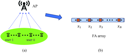
Figure 1: Illustration of the considered system model.

As shown in Fig. 1(b), the AP is assumed to be equipped with an FA array, where the positions of the $N$ FAs can be adjusted within a one-dimensional line segment of length $L$. Let $x_{n}\in[0,L]$ denote the position of the $n$-th FA, and $\bm{x}=[x_{1},\cdots,x_{N}]^{T}$ the APV of all $N$ FAs, satisfying $0\leq x_{1}<\cdots<x_{N}\leq L$ without loss of generality. Consequently, the receive steering vector of the FA array can be expressed as a function of the APV $\bm{x}$ and the steering angle $\theta$:

$$\bm{a}(\bm{x},\theta)=\left[e^{j\frac{2\pi}{\lambda}x_{1}\cos(\theta)},\cdots,e^{j\frac{2\pi}{\lambda}x_{N}\cos(\theta)}\right]^{T},$$ (2)

where $\lambda$ denotes the wavelength.

Let $\bm{h}_{k}\in{\cal C}^{N\times 1}$ denote the channel from user $k$ to AP, given by

$$\bm{h}_{k}=\alpha_{k}\bm{a}(\bm{x},\theta_{k}),$$ (3)

where $\alpha_{k}$ and $\theta_{k}$ represent the propagation gain and angle of arrival (AoA) of the line-of-sight (LoS) path, respectively. Given $\{\bm{h}_{k}\}$, we can express the received signal at AP as follows:

$$\bm{y}=\sum\limits_{k=1}^{K}\bm{h}_{k}b_{k}s_{k}+\bm{z},$$ (4)

where $b_{k}$ is the transmit equalization coefficient of user $k$, $\forall k\in\mathcal{K}$, and $\bm{z}\sim{\cal CN}(\bm{0},\sigma^{2}\bm{I})$ is the additive white Gaussian noise at AP.

With a decoding vector $\bm{m}\in{\cal C}^{N\times 1}$ at AP, the estimated target function is given by

$$\hat{s}=\bm{m}^{H}\bm{y}=\sum\limits_{k=1}^{K}\bm{m}^{H}\bm{h}_{k}b_{k}s_{k}+\bm{m}^{H}\bm{z}.$$ (5)

II-B Problem Formulation

In this paper, we aim to minimize the distortion between the target and the estimated function variables, which is measured by the MSE defined as follows:

$$\mathbb{MSE} \triangleq{\mathbb{E}}[|\hat{s}-s|^{2}]$$

$$={\mathbb{E}}\left[\left|\sum\limits_{k=1}^{K}\left(\bm{m}^{H}\bm{h}_{k}b_{k}-1\right)s_{k}+\bm{m}^{H}\bm{z}\right|^{2}\right]$$

$$=\sum\limits_{k=1}^{K}\left|\bm{m}^{H}\bm{h}_{k}b_{k}-1\right|^{2}+\sigma^{2}\|\bm{m}\|^{2}.$$ (6)

To minimize the MSE, we need to seek the optimal $\bm{b}\triangleq[b_{1},\cdots,b_{K}]^{T}$, $\bm{m}$, and $\bm{x}$, leading to the following optimization problem:

$$\min\limits_{\bm{b},\bm{m},\bm{x}} ~{}\sum\limits_{k=1}^{K}\left|\bm{m}^{H}\bm{h}_{k}(\bm{x})b_{k}-1\right|^{2}+\sigma^{2}\|\bm{m}\|^{2}$$ (7a)

s.t. $$~{}~{}|b_{k}|^{2}\leq P_{k},~{}\forall k\in\mathcal{K},$$ (7b)

$$~{}~{}x_{1}\geq 0,x_{N}\leq L,$$ (7c)

$$~{}~{}x_{n}-x_{n-1}\geq L_{0},~{}\forall n=2,\cdots,N,$$ (7d)

where (7b) accounts for the maximum transmission power constraint for each user, (7c) guarantees that the FAs are moved within the feasible region $[0,L]$, and (7d) ensures that the distance between two adjacent FAs is no less than $L_{0}$ to avoid antenna coupling.

III Transceiver and APV Design

In the sequel, we adopt the AO technique to resolve the coupling between $\bm{b}$, $\bm{m}$, and $\bm{x}$ in (7), and optimize one variable at a time with others being fixed.

1) Optimization of $\bm{b}$: The associated optimization problem with respect to $\bm{b}$ is given by

$$\min\limits_{\bm{b}} ~{}\sum\limits_{k=1}^{K}\left|\bm{m}^{H}\bm{h}_{k}b_{k}-1\right|^{2}$$ (8a)

s.t. $$~{}~{}|b_{k}|^{2}\leq P_{k},~{}\forall k\in\mathcal{K}.$$ (8b)

It is observed that $b_{1},\cdots,b_{K}$ in (8) are decoupled and can be decomposed into $K$ subproblems. The subproblem associated with $b_{k}$, $\forall k\in\mathcal{K}$, is given by

$$\min\limits_{b_{k}} ~{}\left|\bm{m}^{H}\bm{h}_{k}b_{k}-1\right|^{2}$$ (9a)

s.t. $$~{}~{}|b_{k}|^{2}\leq P_{k},$$ (9b)

which is a convex QCQP and can be solved optimally using the Karush-Kuhn-Tucker (KKT) conditions, as detailed below.

Firstly, the Lagrangian associated with (9) can be expressed as follows:

$${\mathcal{L}}_{1}(b_{k},\mu_{k})=\left|\bm{m}^{H}\bm{h}_{k}b_{k}-1\right|^{2}+\mu_{k}\left(|b_{k}|^{2}-P_{k}\right),$$ (10)

where $\mu_{k}\geq 0$ is the Lagrange multiplier. The KKT conditions of (10) are given by

$$\frac{\partial\mathcal{L}_{1}}{\partial b^{*}_{k}}=|\bm{m}^{H}\bm{h}_{k}|^{2}b_{k}-\bm{h}^{H}_{k}\bm{m}+\mu_{k}b_{k}=0,$$ (11a)

$$\mu_{k}\left(|b_{k}|^{2}-P_{k}\right)=0,$$ (11b)

$$|b_{k}|^{2}\leq P_{k}.$$ (11c)

From (11a), we can derive the optimal $b_{k}$ as follows:

$$b_{k}^{\star}=\frac{\bm{h}^{H}_{k}\bm{m}}{|\bm{m}^{H}\bm{h}_{k}|^{2}+\mu_{k}},$$ (12)

where the nonnegative Lagrange multiplier $\mu_{k}$ should be chosen to satisfy (11b) and (11c). By substituting (12) into (11b), we obtain that

$$\mu_{k}^{\star}=\max\left(\frac{|\bm{m}^{H}\bm{h}_{k}|}{\sqrt{P_{k}}}-|\bm{m}^{H}\bm{h}_{k}|^{2},0\right).$$ (13)

2) Optimization of $\bm{m}$: The associated optimization problem with respect to $\bm{m}$ is given by

$$\min\limits_{\bm{m}}~{}\mathbb{MSE}(\bm{m})=\sum\limits_{k=1}^{K}\left|\bm{m}^{H}\bm{h}_{k}b_{k}-1\right|^{2}+\sigma^{2}\|\bm{m}\|^{2}.$$ (14)

It is observed that (14) is a (convex) least squares problem, and the optimal $\bm{m}$ can be found by setting the derivative $\mathbb{MSE}(\bm{m})/\partial\bm{m}^{*}$ to zero. Specifically,

$$\frac{\mathbb{MSE}(\bm{m})}{\partial\bm{m}^{*}}=\sum\limits_{k=1}^{K}\left(|b_{k}|^{2}\bm{h}_{k}\bm{h}_{k}^{H}\bm{m}-b_{k}\bm{h}_{k}\right)+\sigma^{2}\bm{m}=\bm{0},$$ (15)

which yields

$$\bm{m}^{\star}=\left(\sigma^{2}\bm{I}+\sum\limits_{k=1}^{K}|b_{k}|^{2}\bm{h}_{k}\bm{h}_{k}^{H}\right)^{-1}\sum\limits_{k=1}^{K}b_{k}\bm{h}_{k}.$$ (16)

3) Optimization of $\bm{x}$: The associated optimization problem with respect to $\bm{x}$ is given by

$$\min\limits_{\bm{x}} ~{}\sum\limits_{k=1}^{K}\left|\bm{m}^{H}\bm{a}(\bm{x},\theta_{k})\alpha_{k}b_{k}-1\right|^{2}$$ (17a)

s.t. $$~{}~{}\eqref{OP0-APVCons1},~{}\eqref{OP0-APVCons2}.$$ (17b)

Before solving (17), we rewrite (17a) into a more tractable form. Firstly, we expand $\sum\nolimits_{k=1}^{K}\left|\bm{m}^{H}\bm{a}(\bm{x},\theta_{k})\alpha_{k}b_{k}-1\right|^{2}$ as follows:

$$\sum\limits_{k=1}^{K}\Big{(}|\bm{w}_{k}^{H}\bm{a}(\bm{x},\theta_{k})|^{2}-\bm{w}_{k}^{H}\bm{a}(\bm{x},\theta_{k})-\bm{a}^{H}(\bm{x},\theta_{k})\bm{w}_{k}+1\Big{)},$$

where $\bm{w}^{H}_{k}\triangleq\alpha_{k}b_{k}\bm{m}^{H}$, $\forall k\in\mathcal{K}$. By denoting the $n$-th entry in $\bm{w}_{k}$ as $w_{k,n}=|w_{k,n}|e^{j\angle w_{k,n}}$, $\forall n\in\mathcal{N}$, we can then rewrite $\bm{w}_{k}^{H}\bm{a}(\bm{x},\theta_{k})$ as follows:

$$\bm{w}_{k}^{H}\bm{a}(\bm{x},\theta_{k}) =\sum\limits_{n=1}^{N}w^{*}_{k,n}e^{j\phi_{k}x_{n}}$$

$$=\sum\limits_{n=1}^{N}|w_{k,n}|e^{j(\phi_{k}x_{n}-\angle w_{k,n})},$$ (18)

where $\phi_{k}=\frac{2\pi}{\lambda}\cos(\theta_{k})$. Given (III), we can rewrite $F_{k}(\bm{x})\triangleq|\bm{w}_{k}^{H}\bm{a}(\bm{x},\theta_{k})|^{2}$ and $G_{k}(\bm{x})\triangleq\bm{w}_{k}^{H}\bm{a}(\bm{x},\theta_{k})+\bm{a}^{H}(\bm{x},\theta_{k})\bm{w}_{k}$ as follows:

$$F_{k}(\bm{x}) \triangleq|\bm{w}_{k}^{H}\bm{a}(\bm{x},\theta_{k})|^{2}=\left|\sum\limits_{n=1}^{N}|w_{k,n}|e^{j(\phi_{k}x_{n}-\angle w_{k,n})}\right|^{2}$$

$$=\sum\limits_{n=1}^{N}\sum\limits_{l=1}^{N}|w_{k,n}w_{k,l}|e^{j[\phi_{k}(x_{n}-x_{l})-(\angle w_{k,n}-\angle w_{k,l})]}$$

$$=\sum\limits_{n=1}^{N}\sum\limits_{l=1}^{N}|w_{k,n}w_{k,l}|\cos[q_{k}(x_{n},x_{l})],$$ (19)

$$G_{k}(\bm{x}) \triangleq\bm{w}_{k}^{H}\bm{a}(\bm{x},\theta_{k})+\bm{a}^{H}(\bm{x},\theta_{k})\bm{w}_{k}$$

$$=2\sum\limits_{n=1}^{N}|w_{k,n}|\cos(\phi_{k}x_{n}-\angle w_{k,n}),$$ (20)

where $q_{k}(x_{n},x_{l})=\phi_{k}(x_{n}-x_{l})-(\angle w_{k,n}-\angle w_{k,l})$.

Given (19) and (20), we successfully transform (17a) into a more tractable form. However, the function $\sum\nolimits_{k=1}^{K}[F_{k}(\bm{x})-G_{k}(\bm{x})]$ is still highly non-convex, and thus we employ the PDIP method to obtain a locally optimal $\bm{x}$, as detailed in Appendix A.

The proposed transceiver and APV design approach is outlined in Algorithm 1. Moreover, the convergence of Algorithm 1 is illustrated in the following theorem.

Theorem 1

Algorithm 1 converges to a locally optimal point of problem (7) after several iterations.

Proof:

The proof is analogous to that for [Algorithm 1, 9], and thus we omit it for brevity. ∎

Algorithm 1 Pseudo-Code for the Proposed Transceiver and APV Design

1:Given $b_{k}=\sqrt{P_{k}}$, $\forall k\in\mathcal{K}$, and $x_{n}=\frac{Ln}{N+1}$, $\forall n\in\{1,\cdots,N\}$;

2:while not converge do

3:     Update $\bm{m}$ through (16);

4:     Update $\bm{b}$ through solving (12);

5:     Update $\bm{x}$ via the PDIP method.

6:end while

IV Numerical Results

In this section, we present numerical results demonstrating the effectiveness of introducing FA arrays in enhancing AirComp performance. We set $L_{0}=0.5\lambda$, $L=8\lambda$, $P_{k}=P_{0}$, $\forall k\in\mathcal{K}$, and $\text{SNR}\triangleq P_{0}/\sigma^{2}$. Moreover, the following benchmark schemes are considered for comparison.

• Fixed-Position Antenna (FPA): The $N$ FAs are fixed and uniformly distributed in the feasible region $[0,L]$, i.e., the APV is fixed to $\bm{x}=\left[\frac{L}{N+1},\cdots,\frac{NL}{N+1}\right]^{T}$. The optimal $\bm{b}$ and $\bm{m}$ are obtained by recursively running (12) and (16) until convergence.

• SCA: Referring to [11], the non-convex optimization problem (17) for $\bm{x}$ can also be solved by using the successive convex approximation (SCA) technique, while the optimization procedures for $\bm{b}$ and $\bm{m}$ remain unchanged, i.e., (12) and (16), respectively. For more details, refer to Appendix B.

In Fig. 2, we show the MSE performance across iterations for the aforementioned schemes under different SNR levels. From this figure, we immediately observe that our proposed scheme significantly outperforms the FPA scheme for both SNR values. In contrast, the SCA scheme only achieves marginal improvement compared to the FPA scheme, particularly when $\text{SNR}=0$ dB, which can be attributed to the relaxations used in constructing convex surrogate functions for (17a). Additionally, we observe from this figure that all three schemes exhibit rapid convergence.

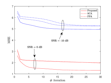
Figure 2: MSE versus the number of iterations under different SNRs, where $N=8$ and $K=10$.

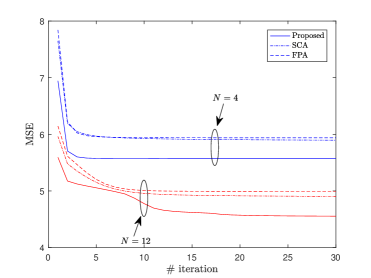
Figure 3: MSE versus the number of iterations for different numbers of FAs $N$, where $\text{SNR}=-10$ dB, and $K=10$.

Fig. 3 depicts the MSE performance for the three aforementioned schemes across different numbers of FAs, i.e., $N$. As expected, the MSE performance consistently decreases across all three schemes as $N$ increases from $4$ to $12$. It is also observed that our proposed scheme showcases a significant advantage over the FPA scheme at both $N=4$ and $N=12$, again highlighting the benefits of optimizing the positions of FAs.

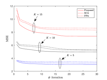
Figure 4: MSE versus the number of iterations for different numbers of users, where $N=8$ and $\text{SNR}=-10$ dB.

In Fig. 4, the MSE performance for the three aforementioned schemes across different user numbers, i.e., $K$, is presented. Unsurprisingly, the MSE performance consistently rises across all three schemes as $K$ increases. Notably, we also observe the consistent outperformance of the proposed scheme compared to the two benchmark schemes, with the performance gap widening as $K$ increases.

V Conclusions

In this paper, we studied an FA array-enhanced AirComp system. Compared to traditional FPAs, FAs provide new DoFs through antenna movements, thus offering the potential for improved performance. As such, we jointly optimized the transceiver design and APV to minimize the MSE between target and estimated function values. Numerical results demonstrated that FA arrays with our proposed transceiver and APV design significantly outperformed traditional FPAs in terms of MSE.

Appendix A

For ease of exposition, we rewrite $x_{1}\geq 0$, $x_{n}\leq L$, and (7d) as follows:

$$f_{1}(\bm{x})=-\bm{e}^{T}_{1}\bm{x}\leq 0,$$

$$f_{2}(\bm{x})=\bm{e}^{T}_{N}\bm{x}-L\leq 0,$$

$$f_{3}(\bm{x})=(\bm{e}_{1}-\bm{e}_{2})^{T}\bm{x}+L_{0}\leq 0,$$

$$~{}~{}\vdots$$

$$f_{N+1}(\bm{x})=(\bm{e}_{N-1}-\bm{e}_{N})^{T}\bm{x}+L_{0}\leq 0,$$

where $\bm{e}_{n}$ denotes the $n$-th column of $\bm{I}_{N}$, $\forall n\in\{1,\cdots,N\}$. Given $g(\bm{x})\triangleq\sum\nolimits_{k=1}^{K}[F_{k}(\bm{x})-G_{k}(\bm{x})]$ and $f_{i}(\bm{x})$, $\forall i=1,\cdots,N+1$, we rewrite (17) as follows:

$$\min\limits_{\bm{x}} ~{}g(\bm{x})$$ (21a)

s.t. $$~{}f_{i}(\bm{x})\leq 0,~{}\forall i=1,\cdots,N+1.$$ (21b)

The Lagrangian associated with (21) is given by

$$\mathcal{L}_{2}(\bm{x},\bm{\nu})=g(\bm{x})+\bm{f}(\bm{x})^{T}\bm{\nu},$$ (22)

where $\bm{\nu}=[\nu_{1},\cdots,\nu_{N+1}]^{T}$ is the Lagrange multiplier and $\bm{f}(\bm{x})\triangleq[f_{1}(\bm{x}),\cdots,f_{N+1}(\bm{x})]^{T}$. According to [14], the dual residual and the centrality residual corresponding to (22) can be expressed as follows:

$$\bm{r}_{\rm dual}(\bm{x},\bm{\nu})\triangleq\nabla g(\bm{x})+D\bm{f}(\bm{x})^{T}\bm{\nu},$$ (23)

$$\bm{r}_{\rm cent}(\bm{x},\bm{\nu})\triangleq-{\rm diag}(\bm{\nu})\bm{f}(\bm{x})-(1/\delta)\bm{1},$$ (24)

where $D\bm{f}(\bm{x})^{T}=[\nabla f_{1}(\bm{x}),\cdots,\nabla f_{N+1}(\bm{x})]$, and $\delta>0$. If the current point $\bm{x}$ and $\bm{\nu}$ satisfy $\bm{r}_{\rm dual}(\bm{x},\bm{\nu})=\bm{0}$, and $\bm{r}_{\rm cent}(\bm{x},\bm{\nu})=\bm{0}$, then $\bm{x}$ is primal feasible, and $\bm{\nu}$ is dual feasible, with duality gap no less than $(N+1)/\delta$. Otherwise, we have to proceed with the iteration, and the primal-dual search direction $(\Delta\bm{x}_{\rm pd},\Delta\bm{\nu}_{\rm pd})$ is determined by the solution of the following equation:

$$\begin{bmatrix}\nabla^{2}g(\bm{x})+\sum\nolimits_{i=1}^{N+1}\nu_{i}\nabla^{2}f_{i}(\bm{x})&D\bm{f}(\bm{x})^{T}\\[4.30554pt] -{\rm diag}(\bm{\nu})D\bm{f}(\bm{x})&-{\rm diag}(\bm{f}(\bm{x}))\end{bmatrix}\begin{bmatrix}\Delta\bm{x}\\[4.30554pt] \Delta\bm{\nu}\end{bmatrix}$$

$$=-\begin{bmatrix}\bm{r}_{\rm dual}(\bm{x},\bm{\nu})\\[4.30554pt] \bm{r}_{\rm cent}(\bm{x},\bm{\nu})\end{bmatrix}.~{}~{}~{}~{}~{}~{}~{}$$ (25)

The overall procedures of the PDIP method are summarized in Algorithm 2.

Algorithm 2 Pseudo-Code for Solving (21) with the PDIP Method

1:Choose $\bm{x}$ that satisfies $\bm{f}(\bm{x})\prec\bm{0}$, $\bm{\nu}\succ\bm{0}$, $\eta\triangleq-\bm{f}(\bm{x})^{T}\bm{\nu}$, $\epsilon>0$, $\epsilon_{\rm feas}>0$, and $\xi>1$.

2:while $\|\bm{r}_{\rm dual}\|>\epsilon_{\rm feas}$ or $\eta>\epsilon$ do

3:     Define $\delta=\xi(N+1)/\eta$;

4:     Compute $(\Delta\bm{x}_{\rm pd},\Delta\bm{\nu}_{\rm pd})$ via solving (A);

5:     Determine step size $\gamma$ via backtracking line search;

6:     Update $(\bm{x},\bm{\nu})\leftarrow(\bm{x},\bm{\nu})+\gamma(\Delta\bm{x}_{\rm pd},\Delta\bm{\nu}_{\rm pd})$;

7:     Compute $\eta=-\bm{f}(\bm{x})^{T}\bm{\nu}$.

8:end while

Appendix B

Motivated by [11], we construct convex surrogate functions to locally approximate $F_{k}(\bm{x})$ and $G_{k}(\bm{x})$ based on the second-order Taylor expansion. Specifically, for a given $u_{0}\in\mathcal{R}$, the second-order Taylor expansion of $\cos(u)$ is given by

$$\cos(u)\approx\cos(u_{0})-\sin(u_{0})(u-u_{0})-\frac{1}{2}\cos(u_{0})(u-u_{0})^{2}$$ (26)

Since $-1\leq\cos(u_{0})\leq 1$, $\forall u_{0}\in\mathcal{R}$, we have

$$\cos(u)\overset{(a)}{\leq}\cos(u_{0})-\sin(u_{0})(u-u_{0})+\frac{1}{2}(u-u_{0})^{2},$$ (27)

$$\cos(u)\overset{(b)}{\geq}\cos(u_{0})-\sin(u_{0})(u-u_{0})-\frac{1}{2}(u-u_{0})^{2},$$ (28)

where $(a)$ is due to $\cos(u_{0})\geq-1$, and $(b)$ is due to $\cos(u_{0})\leq 1$. Denote the $i$-th iteration of SCA as $\bm{x}^{i}=[x^{i}_{1},\cdots,x^{i}_{N}]^{T}$. Given (27) and letting $u\leftarrow\phi_{k}(x_{n}-x_{l})-(\angle w_{k,n}-\angle w_{k,l})$, $u_{0}\leftarrow\phi_{k}(x^{i}_{n}-x^{i}_{l})-(\angle w_{k,n}-\angle w_{k,l})$, we derive an upper bound for $F_{k}(\bm{x})$, given by

$$F_{k}(\bm{x})\leq F_{k}(\bm{x}|\bm{x}^{i})=\bm{x}^{T}\bm{A}_{k}\bm{x}-(\bm{v}^{i}_{k})^{T}\bm{x}+C^{i}_{k},$$ (29)

where $\bm{A}_{k}$, $\bm{v}^{i}_{k}$, and $C^{i}_{k}$ are respectively given by

$$\bm{A}_{k}=\phi_{k}^{2}\left(\bar{w}_{k,0}{\rm diag}(\bar{\bm{w}}_{k})-\bar{\bm{w}}_{k}\bar{\bm{w}}_{k}^{T}\right),$$

$$[\bm{v}^{i}_{k}]_{n}=\sum\limits_{l=1}^{N}\left(\varphi^{i}_{k,n,l}-\varphi^{i}_{k,l,n}\right),$$

$$\varphi^{i}_{k,n,l}=|w_{k,n}w_{k,l}|[\sin(q_{k}(x_{n}^{i},x_{l}^{i}))\phi_{k}+\phi^{2}_{k}(x^{i}_{n}-x^{i}_{l})],$$

$$C^{i}_{k}=\sum\limits_{n=1}^{N}\sum\limits_{l=1}^{N}|w_{k,n}w_{k,l}|[0.5\phi^{2}_{k}(x^{i}_{n}-x^{i}_{l})^{2}$$

$$~{}~{}~{}~{}~{}~{}~{}+\cos(q_{k}(x_{n}^{i},x_{l}^{i}))+\sin(q_{k}(x_{n}^{i},x_{l}^{i}))\phi_{k}(x^{i}_{n}-x^{i}_{l})],$$

where $\bar{w}_{k,0}=\sum\nolimits_{n=1}^{N}|w_{k,n}|$, $\bar{\bm{w}}_{k}=|\bm{w}_{k}|$, and $q_{k}(x_{n}^{i},x_{l}^{i})=\phi_{k}(x^{i}_{n}-x^{i}_{l})-(\angle w_{k,n}-\angle w_{k,l})$.

On the other hand, given (28) and letting $u\leftarrow\phi_{k}(x_{n}-x_{l})-(\angle w_{k,n}-\angle w_{k,l})$, $u_{0}\leftarrow\phi_{k}(x^{i}_{n}-x^{i}_{l})-(\angle w_{k,n}-\angle w_{k,l})$, we derive a lower bound for $G_{k}(\bm{x})$, given by

$$G_{k}(\bm{x})\geq G_{k}(\bm{x}|\bm{x}^{i})=-\bm{x}^{T}\tilde{\bm{A}}_{k}\bm{x}+2(\tilde{\bm{v}}^{i}_{k})^{T}\bm{x}+2\tilde{C}^{i}_{k},$$ (30)

where $\tilde{\bm{A}}_{k}$, $\tilde{\bm{v}}^{i}_{k}$, and $\tilde{C}^{i}_{k}$ are respectively given by

$$\tilde{\bm{A}}_{k}=\phi_{k}^{2}{\rm diag}(\bm{\bar{w}}_{k}),$$

$$[\tilde{\bm{v}}^{i}_{k}]_{n}=|w_{k,n}|[\phi^{2}_{k}x^{i}_{n}-\sin(\phi_{k}x_{n}^{i}-\angle w_{k,n})\phi_{k}],$$

$$\tilde{C}^{i}_{k}=\sum\limits_{n=1}^{N}|w_{k,n}|[\cos(\phi_{k}x_{n}^{i}-\angle w_{k,n})$$

$$~{}~{}~{}~{}+\sin(\phi_{k}x_{n}^{i}-\angle w_{k,n})\phi_{k}x^{i}_{n}-0.5\phi^{2}_{k}(x^{i}_{n})^{2}].$$

Given (29) and (30), the $(i+1)$-th iteration of SCA can be formulated as follows:

$$\min\limits_{\bm{x}} ~{}\bm{x}^{T}\bm{A}\bm{x}-(\bm{v}^{i})^{T}\bm{x}+C^{i}$$ (31a)

s.t. $$~{}\eqref{OP0-APVCons1},~{}\eqref{OP0-APVCons2},$$ (31b)

where $\bm{A}=\sum\nolimits_{k=1}^{K}(\bm{A}_{k}+\tilde{\bm{A}}_{k})$, $\bm{v}^{i}=\sum\nolimits_{k=1}^{K}(\bm{v}^{i}_{k}+2\tilde{\bm{v}}^{i}_{k})$, and $C^{i}=\sum\nolimits_{k=1}^{K}(C^{i}_{k}-2\tilde{C}^{i}_{k}+1)$. Since (7c) and (7d) are linear constraints and $\bm{A}$ is a positive semi-definite matrix, therefore (31) is a convex optimization problem and can be efficiently solved using CVX [15].

References

• [1] G. Zhu, J. Xu, K. Huang, and S. Cui, “Over-the-air computing for wireless data aggregation in massive IoT,” IEEE Wireless Communications, vol. 28, no. 4, pp. 57-65, August 2021.
• [2] Z. Wang, Y. Zhao, Y. Zhou, et al., “Over-the-air computation: Foundations, technologies, and applications,” 2022, arXiv: 2210.10524.
• [3] X. Cao, G. Zhu, J. Xu, and K. Huang, “Optimized power control for over-the-air computation in fading channels,” IEEE Transactions on Wireless Communications, vol. 19, no. 11, pp. 7498-7513, Nov. 2020.
• [4] W. Liu, X. Zang, Y. Li, and B. Vucetic, “Over-the-air computation systems: optimization, analysis and scaling laws,” IEEE Transactions on Wireless Communications, vol. 19, no. 8, pp. 5488-5502, Aug. 2020.
• [5] L. Chen, X. Qin, and G. Wei, “A uniform-forcing transceiver design for over-the-air function computation,” IEEE Wireless Communications Letters, vol. 7, no. 6, pp. 942-945, Dec. 2018.
• [6] G. Zhu, and K. Huang, “MIMO over-the-air computation for high-mobility multimodal sensing,” IEEE Internet Things Journal, vol. 6, no. 4, pp. 6089–6103, Aug. 2019.
• [7] W. Fang, Y. Jiang, Y. Shi, et al., “Over-the-air computation via reconfigurable intelligent surface,” IEEE Transactions on Communications, vol. 69, no. 12, pp. 8612-8626, Dec. 2021.
• [8] X. Zhai, G. Han, et al., “Simultaneously transmitting and reflecting (STAR) RIS assisted over-the-air computation systems,” IEEE Transactions on Communications, vol. 71, no. 3, pp. 1309-1322, March 2023.
• [9] D. Zhang, M. Xiao, M. Skoglund, and H. V. Poor, “Beamforming design for active RIS-aided over-the-air computation,” 2023, arXiv:2311.18418.
• [10] K. K. Wong, W. K. New, X. Hao, et al., “Fluid antenna system-Part I: Preliminaries,” IEEE Communications Letters, vol. 27, no. 8, pp. 1919-1923, August 2023.
• [11] W. Ma, L. Zhu, and R. Zhang, “Multi-beam forming with movable-antenna array,” 2023, arXiv:2311.03775.
• [12] K. K. Wong, A. Shojaeifard, K. F. Tong, and Y. Zhang, “Fluid antenna systems,” IEEE Transactions on Wireless Communications, vol. 20, no. 3, pp. 1950-1962, March 2021.
• [13] Y. Wu, D. Xu, D. W. K. Ng, et al., “Movable antenna-enhanced multiuser communication: Optimal discrete antenna positioning and beamforming,” 2023, arXiv:2308.02304.
• [14] S. Boyd, and L. Vandenberghe, Convex Optimization. Cambridge University Press, 2004.
• [15] M. Grant, and Stephen Boyd, CVX: Matlab software for disciplined convex programming, version 2.0 beta. http://cvxr.com/cvx, Sept. 2013.