Impact of anisotropic cosmic-ray transport on the gamma-ray signatures in the Galactic Center

Abstract

The very high energy (VHE) emission of the Central Molecular Zone (CMZ) is rarely modelled in 3D. Most approaches describe the morphology in 1D or simplify the diffusion to the isotropic case. In this work we show the impact of a realistic 3D magnetic field configuration and gas distribution on the VHE gamma-ray distribution of the CMZ. We solve the 3D cosmic-ray transport equation with an anisotropic diffusion tensor using the approach of stochastic differential equations as implemented in the CRPropa framework. We test two different source distributions for five different anisotropies of the diffusion tensor, covering the range of effectively fieldline-parallel diffusion to isotropic diffusion. Within the tested magnetic field configuration the anisotropy of the diffusion tensor is close to the isotropic case and three point sources within the CMZ are favoured. Future missions like the upcoming CTA will reveal more small-scale structures which are not jet included in the model. Therefor a more detailed 3D gas distribution and magnetic field structure will be needed.

1 Introduction

The Galactic Center (GC) is one of the most extreme and close by astrophysical environments and of particular interest for studies of non-thermal processes. The GC has been studied in all wavelengths from radio (Heywood et al., 2022) to high- (Ajello et al., 2016; Di Mauro, 2021) and very high energy (VHE) $\gamma$-rays (Abramowski et al., 2016; Abdalla et al., 2018; Acciari et al., 2020; Adams et al., 2021). The observed outflows at gamma-ray (Ackermann et al., 2014), X-ray (Sofue, 2000), microwave (Finkbeiner, 2004; Planck Collaboration et al., 2013) and radio wavelength (Pedlar et al., 1989) as well as the small-scale structures like the non-thermal filaments and the molecular clouds (see Henshaw et al. (2023) for a review) are in need of proper modelling.

The observation of VHE gamma-rays, first reported by the High Energy Stereoscopic System (H.E.S.S.) (Abramowski et al., 2016), hints towards the acceleration of cosmic-ray (CR) protons to energies up to PeV. The GC is one of a few so-called PeVatrons known in our Milky Way. The diffuse VHE gamma-ray emission in the GC has been spatially correlated with the dense gas of the central molecular zone (CMZ) and seems to be consistent with the injection of CRs by a steady state source located at the GC (Abdalla et al., 2018). In that analysis the authors use the projected distribution of the H₂ column density inferred by the observation of the CS(1-0) line multiplied by a parameterised source profile of a Gaussian or a $1/r$-CR density profile. This approach of modelling the CR transport neglects the existence of small-scale features in the 3D gas distribution as well as in the magnetic field.

The first attempt to model the gamma-ray emission of the CMZ using a three-dimensional gas distribution was carried out by Scherer et al. (2022). These authors probe whether the gas has an inner cavity or not. In lack of a three-dimensional magnetic field the authors assume isotropic diffusion for a Kraichnan spectrum of magnetic turbulence. Recently, these authors tested more realistic source distributions and a two-zone diffusion model (Scherer et al., 2023).

In this paper, we use the results of Guenduez et al. (2020) in order to perform diffusive 3D cosmic-ray propagation in the CMZ. We include the three-dimensional gas distribution for interactions and distinguish between parallel and perpendicular diffusion. Further, we test different source injection models, related to point sources inside the CMZ and a sea of Galactic cosmic rays.

The paper is organised as follows: in section 2 the Galactic Center environment and its observations are summarized. In section 3 the transport model and simulation setup is presented and in Section 4 the simulation results are compared to the observed data. Finally, in section 5 a concluding discussion and an outlook is given.

2 Galactic Center environment

2.1 VHE $\gamma$-ray observation

The Galactic Center has been studied in VHE $\gamma$-rays ($>$ 100 GeV). The first detection of $\sim 100$ TeV $\gamma$-ray emission by Abramowski et al. (2016) provided first evidence for the existence of a PeVatron in the Galactic Center region. In Abdalla et al. (2018), H.E.S.S. quantified the spatial distribution of the diffuse $\gamma$-rays and the corresponding spectrum. Evan MAGIC (Acciari et al., 2020) and VERITAS (Adams et al., 2021) have observed the CMZ. High energy $\gamma$-ray emission from the Galactic Center is even detected at GeV energies by Fermi. As the Galactic Center region shows deviations from the typical expectation of cosmic-ray transport (Ackermann et al., 2017) and Dark Matter has been proposed as a possible contributor at GeV energies (Goodenough & Hooper, 2009; Daylan et al., 2016). At $>100$ TeV $\gamma$-ray energies, LHASSO has reported on the detection of photons from the Galactic Plane (Cao et al., 2023). The IceCube collaboration also reported in the first observation of the Galactic Plane in high-energy neutrinos, which represents unambiguous proof for the signatures of hadronic cosmic rays (Abbasi et al., 2023). At this point, the exact contribution to the Galactic emission from the Galactic Center region cannot be quantified.

2.2 Gas distribution

The three-dimensional gas distribution of the CMZ is not well known, and the models are quite uncertain. We use the HI and H₂ CMZ components of the model by Ferrière et al. (2007). In contrast to the observed latitudinal profile of the diffuse $\gamma$-ray emission, the gas model shows a significantly smaller scale height of the disc (see Fig. 1). Therefore, we change the scale height of the gas distribution to $H_{c}=30\,\mathrm{pc}$, which is near the upper limit of the observational uncertainties.

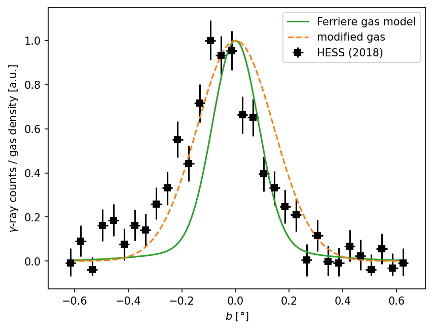
Figure 1: Comparison between the latitudinal profile ($b$) of the observed diffuse $\gamma$-ray flux (black squares) by H.E.S.S. (Abdalla et al., 2018) and model of the gas distribution (solid green line) by Ferrière et al. (2007). The orange dashed line corresponds to the gas distribution using a larger parameter for the scale height of $H_{c}=30\,\mathrm{pc}$.

2.3 Magnetic field configuration

To determine the local directions of parallel and perpendicular CR transport, the knowledge of the three-dimensional magnetic field configuration is crucial. Here, we use the model proposed by Guenduez et al. (2020) , which is a superposition of a large-scale intercloud (IC) component and more localised contributions. These small-scale components include the eight observed non-thermal filaments (NTF), 12 molecular clouds (MC) and a contribution from Sgr A^∗ . The IC and NTF components are predominantly poloidal while the molecular clouds are torodial. In the MCs the ratio $\eta=B_{r}/B_{\phi}$ between the radial and azimuthal field is fixed to $\eta=0.5$ as suggested in Guenduez et al. (2020). The total magnetic field can be written as

$$\vec{B}_{\mathrm{tot}}=\vec{B}_{\mathrm{IC}}+\sum_{i=1}^{8}\vec{B}_{\mathrm{NTF},i}+\sum_{i=1}^{12}\vec{B}_{\mathrm{MC},i}+\vec{B}_{\mathrm{SgrA^{*}}}\quad.$$ (1)

3 Simulation setup

The transport of Galactic CRs can be described by the Parker equation (see, e.g., Becker Tjus & Merten 2020)

$$\frac{\partial n}{\partial t}=\nabla\hat{\kappa}\nabla n-\frac{\partial}{\partial E}\left[\frac{\mathrm{d}E}{\mathrm{d}t}n\right]+S(\vec{r},E,t)\quad,$$ (2)

where $n=n(\vec{r},E,t)$ denotes the differential number density of CRs per unit volume, energy and time. The diffusion tensor $\hat{\kappa}$ can be diagonalized in the frame of the local magnetic field line. Assuming the magnetic field is pointing in the z-direction $\vec{B}=B\vec{e}_{z}$ the diffusion tensor reads as $\hat{\kappa}=\mathrm{diag}(\kappa_{\perp},\kappa_{\perp},\kappa_{\parallel})$. The details of the assumed diffusion tensor can be seen in sec. 3.1. The last term $S(\vec{r},E,t)$ describes the sources and sinks of CRs, which are described in section 3.2.

The term $\mathrm{d}E/\mathrm{d}t$ quantifies the energy loss of CRs due to the interaction with the interstellar medium (ISM). In this process charged and neutral pions are produced, where the $\pi^{0}$ decay into two photons. We use the hadronic interaction module presented in Hoerbe et al. (2020), which is based on the parameterisation of the differential cross section in Kelner et al. (2006).

We solve the transport equation using the method of stochastic differential equations (SDEs) as implemented in the public transport code CRPropa3.2 (Batista et al., 2016; Merten et al., 2017; Batista et al., 2022). We calculate the steady-state solution following the approach in Merten et al. (2017). Details about the setup are given in section 3.3.

3.1 Diffusion tensor

In general, the diffusive transport of CRs is anisotropic w.r.t. the local magnetic field line. This fact, originally discussed for the transport of CRs in the heliospheric magnetic field (Jokipii, 1966) and, subsequently, refined (e.g., Effenberger et al., 2012a; Shalchi, 2021) as well as quantified (e.g., Reichherzer et al., 2022a), has in recent years also been acknowledged for their Galactic transport (e.g., Effenberger et al., 2012b; Cerri et al., 2017, and references therein). This anisotropy is described by the diffusion tensor $\hat{\kappa}$ in the transport equation (eq. 2).

To quantify the anisotropy the ratio $\epsilon=\kappa_{\perp}/\kappa_{\parallel}$ between the diffusion coefficient perpendicular to the magnetic field line ($\kappa_{\perp}$) and along it ($\kappa_{\parallel}$) is used. In this work we consider five different values ($\epsilon=10^{-3},10^{-2},0.1,0.3,1$) reaching from nearly purely parallel transport to isotropic diffusion. The value of this anisotropy should depend on the local turbulence and can vary spatially (Reichherzer et al., 2020, 2022b, 2022a), but is not known for the GC. Therefore, we test different fixed values to show the impact of this anisotropy parameter.

The energy-scaling for the diffusion coefficients is taken from quasi-linear theory and we normalise the parallel coefficient to match the observed value at Earth. With this the parallel diffusion coefficient reads as

$$\kappa_{\parallel}(E)=6.1\cdot 10^{24}\,\frac{\mathrm{m^{2}}}{\mathrm{s}}\,\cdot\left(\frac{E}{4\,\mathrm{GeV}}\right)^{\frac{1}{3}}\quad,$$ (3)

using the particle energy $E$.

3.2 Sources

As the origin of CRs is not clear we test two different scenarios for the spatial source distribution:

• The first source scenario considers the three observed $\gamma$-ray point sources as observed by H.E.S.S. These are (1) the central source Sgr A^∗ (also called HESS J1745-290), (2) the supernova remnant G0.9+01 and (3) the pulsar HESS J1746-28. In this scenario, the contribution of the individual sources to the total CR luminosity is based on the $\gamma$-ray observation in Abdalla et al. (2018). This corresponds to a fraction of $f_{\mathrm{sgrA}}=0.72$, $f_{\mathrm{G0.9}}=0.22$ and $f_{\mathrm{J1746}}=0.06$.

• In the second source scenario, the full simulation volume is filled by a homogeneous CR source. This distribution could correspond to a CR population which is accelerated outside the GC region and diffused in a long time ago.

An overview of the source position is indicated in fig. 2 by the red stars for the [3sr] scenario and the orange rectangle for the [uni] source scenario.

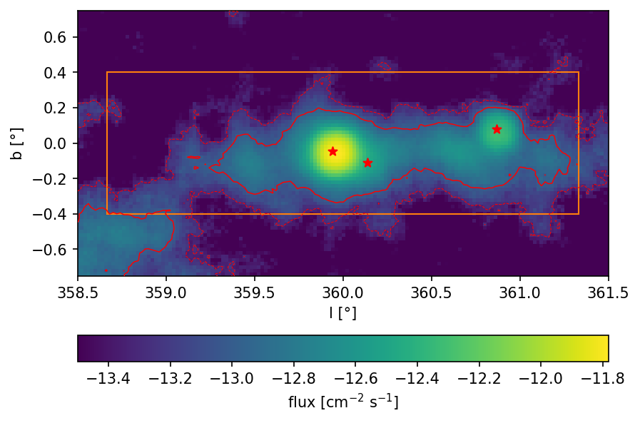
Figure 2: The VHE $\gamma$-ray flux from the CMZ observed by H.E.S.S. Abdalla et al. (2018). The red lines is the contour for $\Phi=10^{-13}\mathrm{cm^{-2}\,s^{-1}}$ (red solid) and $\Phi=5\cdot 10^{-14}\mathrm{cm^{-2}\,s^{-1}}$ (red dashed). The three red stars indicate the position of CR sources. The orange box indicates the simulation volume at $x=0$.

In this work, we restrict our model to only contain protons. These are injected with a flat power-law spectrum $\left.\nicefrac{{\mathrm{d}N}}{{\mathrm{d}E}}\right|_{\mathrm{sim}}\sim E^{-1}$ to ensure equal statistics in each logarithmic energy bin. In the post-processing of the simulation data, the source spectrum is re-weighted to a power law $\left.\nicefrac{{\mathrm{d}N}}{{\mathrm{d}E}}\right|_{s}\sim E^{-\alpha_{s}}$ by assigning a weight

$$w_{i}=\frac{E_{i}^{\alpha_{s}-1}}{\sum_{i}E_{i}^{\alpha_{s}-1}}$$ (4)

to each pseudo-particle, which is called candidate in CRPropa , as presented in Merten et al. (2017).

3.3 CRPropa configuration

The simulation volume is a paraxial box of the size $200\times 400\times 120$ pc³ centered on Sgr A^∗ . For each source configuration and anisotropy parameter, a set of 50 simulations with $N_{\mathrm{sim}}=10^{5}$ primary CRs is run. This splitting is necessary to keep the simulation time per run as well as the amount of data managable .

The details of the used modules for the simulations are summarised in table 1. The output contains all created $\gamma$-rays directly after their production. No propagation and corresponding absorption of $\gamma$-rays is taken into account. To realise this, we use the DetectAll observer and set a veto for nucleons.

module	parameter	value
magnetic field & propagation
CMZField	sub-components	True
DiffusionSDE	precision	$P=10^{-3}$
	minstep	$s_{\mathrm{min}}=10^{-3}\,\mathrm{pc}$
	maxstep	$s_{\mathrm{max}}=10\,\mathrm{pc}$
	anisotropy	$\epsilon\in\left\{10^{-3},10^{-2},0.1,0.3,1\right\}$
observer & output
HDF5Output	enabled columns	TrajectoryLength
		position (source and current)
		energy (source and current)
		serial number
Observer	Particle veto	nucleus, electron, neutrino
	Observer feature	ObserverDetectAll
boundary & break condition
MaximumTrajectoryLength	maximal time	$T_{\mathrm{max}}=500\,\mathrm{kpc}/c$
MinimumEnergy	minimal Energy	$E_{\mathrm{min}}=1\,\mathrm{TeV}$
ParaxialBox	origin	$\vec{o}=(-100,-200,-60)\,\mathrm{pc}$
	size	$\vec{s}=(200,400,120)\,\mathrm{pc}$
ObserverSurface	surface	paraxial box as defined before.
source
SourceParticleType	particle id	proton ($1000010010$)
SourceIsotropicEmission
SourceMultiplePositions	positions	Sgr A∗ : $\vec{r}=(0,8.9,-6.8)\,\mathrm{pc}$
		J1746: $\vec{r}=(0,-20.77,-16.32)\,\mathrm{pc}$
		G0.9+01: $\vec{r}=(0,-129.08,11.87)\,\mathrm{pc}$
or SourceUniformBox	origin / size	$\vec{o}$ and $\vec{s}$ as above

Table 1: CRPropa modules used for the simulation and their input parameters. Module parameters not mentioned are kept at their default values.

The DiffusionSDE module (see Merten et al. (2017) for details) is used to calculate the solution of the transport equation. We use an adaptive step size with a precision of $P=10^{-3}$. The diffusion tensor is described in sec. 3.1. To speed up the simulation in the case of isotropic diffusion, we use a uniform magnetic field in the $z$-direction. In this case, the transport does not depend on the magnetic field configuration, but the adaptive step size method would lower the steps to resolve the curvature of the magnetic field.

We limit the simulation to primary particles with a minimal energy of $E_{\mathrm{min}}=1\,\mathrm{TeV}$ and a maximum simulation time of $T_{\mathrm{max}}=500\,\mathrm{kpc}/{c}$ . Moreover, all particles reaching the boundary of the simulation volume are lost.

3.4 Post processing

After a simulation, all produced $\gamma$-rays are binned and reweighted according to the primary energy. This is done for different power-law indices $\alpha_{s}$ of the source emission. We test $1\leq\alpha_{s}\leq 3$ with steps of $\Delta\alpha_{s}=0.1$. The data are binned in longitude, latitude and energy. In the first step, the binning is done in a much finer resolution than current generation imaging Air Cherenkov telescopes (IACTs) can resolve. We use an angular binning of $\Delta l=0.016^{\circ}$ and $\Delta b=0.01^{\circ}$ to ensure enough statistics in each bin. The resolution effects of the observation are later taken into account by smearing the results. This allows us to compare the data for future telescopes like the upcoming CTA, which will have a two to three times better resolution (The CTA Consortium, 2019). The energy binning is done in the same ranges as in the H.E.S.S. analysis (Abdalla et al., 2018).

4 Results

4.1 Synthetic count maps

Using the produced photons in our simulation, we create synthetic $\gamma$-ray maps by calculating weighted histograms of the longitudinal and latitudinal positions. The weighting takes the injection spectrum $\left.\nicefrac{{\mathrm{d}N}}{{\mathrm{d}E}}\right|_{s}\sim E^{-\alpha_{s}}$ into account. The resulting synthetic count maps for a source index $\alpha_{s}=2.0$ are shown in Fig. 3. In general the maps do not change significantly for different source spectra. To compare our simulation with the observations by H.E.S.S. we apply a Gaussian smearing of $\sigma=0.077^{\circ}$, which is the 68% containment radius of the point spread function (Abdalla et al., 2018). Appendix B contains the same countmaps for the raw data without smearing.

In the case of strong parallel diffusion ($\epsilon=0.001$) the CRs mainly follow the magnetic field lines. This leads to a stronger confinement of CRs in the molecular clouds around Sgr A^∗ and Sgr B2. Therefore also the $\gamma$-ray production is centred near the sources/MCs. For the [3sr] source scenario, the emission around Sgr A^∗ is stronger as the two sources close by emit more CRs. The emission in Sgr B2 shows the direction of the local field line where the CRs diffuse in. By increasing perpendicular diffusion the point like emission is smeared out. The production of $\gamma$-rays at higher latitude becomes more likely and the distribution across the plane is spread out. In the extreme case of isotropic diffusion ($\epsilon=1$) the point source G0.9 is barely visible and hidden by the large-scale diffuse emission.

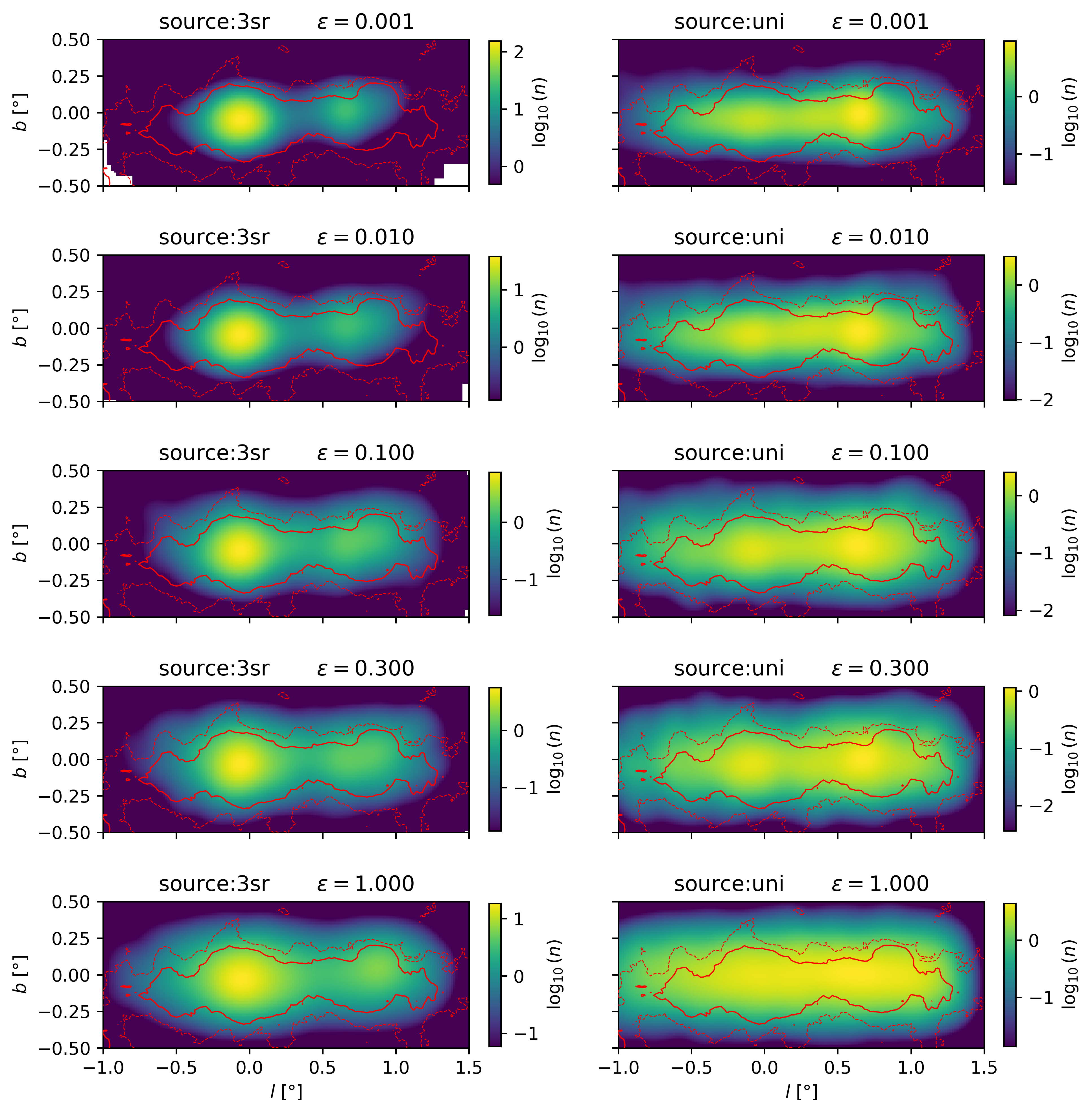
Figure 3: Synthetic $\gamma$-ray maps for a source injection with $\alpha_{s}=2.0$. The first column shows the [3sr] source distribution and the second column the [uni] injection scenario. The row denotes the anisotropy parameter $\epsilon\in\{0.001,0.01,0.1,0.3,1\}$. The thin red lines show the contours of the observed flux by HESS (H. E. S. S. Collaboration et al., 2018) for $\Phi=5\cdot 10^{-14}\,\mathrm{cm^{-2}\,s^{-1}}$ (dashed) and $\Phi=10^{-13}\,\mathrm{cm^{-2}\,s^{-1}}$ (solid).

The $\gamma$-ray maps for the [uni] source injection show an extended disk for all anisotropies. This is expected due to the extended source distribution. Although the sources are distributed homogeneously, a concentration of produced photons around Sgr A^∗ and Sgr B2 is visible. This effect is mainly caused by the stronger magnetic fields in these regions. As these fields are much more twisted the confinement of CRs is more efficient, which also leads to a higher $\gamma$-ray production rate. Especially in the parallel diffusion dominated case ($\epsilon=10^{-3}$) the strongest emission is centred in Sgr B2. For the [uni] source injection the increasing isotropy leads to a wider spread of $\gamma$-rays in latitude, while no clear difference between the longitudinal profiles is visible. Only in the case of isotropic diffusion the peaks of Sgr A^∗ and Sgr B2 are not visible anymore, as this scenario does not depend on the magnetic field configuration.

4.2 Count profiles

To quantify the difference between the distribution of photons we compare our calculated $\gamma$-ray maps with the latitudinal and longitudinal profile presented by H.E.S.S. (see Fig. 4 of Abdalla et al. (2018)). Analogously to the H.E.S.S. data analysis all $\gamma$-rays in a latitudinal (longitudinal) window of $|b|\leq 0.3^{\circ}$ ($|l|\leq 0.5^{\circ}$) are collected. The profiles are calculated on a much finer binning ($\Delta l=0.016^{\circ}$ and $\Delta b=0.01^{\circ}$) and smeared with the H.E.S.S. resolution of $\sigma=0.077^{\circ}$. The simulation data are normalised to match the maximal counts of the latitudinal profile for $b=-0.054^{\circ}$, which is the middle of its peak.

In Fig. 4 the profiles for a source injection with a power law of $\left.\nicefrac{{\mathrm{d}N}}{{\mathrm{d}E}}\right|_{s}\sim E^{-2}$ is shown. The difference for varying the power law slope $\alpha_{s}$ is shown in appendix C. To estimate the agreement between the data and the simulation the reduced $\chi^{2}$

$$\chi^{2}_{\mathrm{red}}=\frac{1}{n-1}\sum_{i=1}^{n}\frac{\left(c_{i}^{(\mathrm{obs})}-c_{i}^{(\mathrm{sim})}\right)^{2}}{\sigma_{i}^{2}}$$ (5)

is calculated. Here $c_{i}$ is the observed or simulated number of counts, $\sigma_{i}$ is the observational uncertainty and $n$ is the total number of data points.

The latitudinal profiles show for both source scenarios a much too thin disk for high anisotropies of the diffusion tensor ($\epsilon=0.001$ or $\epsilon=0.01$). For the [uni] source model, the latitudinal profile is matched best using $\epsilon=0.1$, while the [3sr] model prefers $\epsilon=0.3$. But in both source scenarios, the anisotropic diffusion is favoured over the isotropic case ($\epsilon=1$).

In contrast to the latitudinal profile, where both source scenarios show the same shape, clear differences are visible in the longitudinal profiles (left column of Fig. 4). For the smallest anisotropy, the differences are most dominant. The [3sr] model shows a considerable peaking around the positions of the sources and nearly no $\gamma$-ray production further away. This is expected due to the strong confinement of CRs in the local environment of the sources. The [uni] model shows a nearly smooth distribution over the full range. Only at the position $l=0.657^{\circ}$ a maximum is visible. This can be explained with the strong magnetic field of the MC Sgr B2. With stronger perpendicular diffusion the peak of the [3sr] model is broader. For the [uni] source model the trend is the opposite way. In the case of stronger perpendicular diffusion (up to $\epsilon=0.1$) the longitudinal profile gets higher around Sgr A^∗ , while the peak at Sgr B2 gets spread out. This shift of the peaks in the $\gamma$-ray distribution might result from the small-scale structure of the magnetic field. Especially the position of the MCs and NTFs along the line of sight has a strong impact on the confinement of CRs.

A comparison between the $\chi^{2}_{\mathrm{red}}$ values depending on the anisotropy of the diffusion tensor is shown in Fig. 5.

In the latitudinal comparison the $\chi^{2}_{\mathrm{red}}$ is comparable for all anisotropies $\epsilon\gtrsim 0.1$ and both source distributions. This is expected due to the fixed normalisation of the count rate and only the width of the distribution can change with the anisotropy.

Comparing the longitudinal profiles offers a better discrimination between the source models and anisotropies, as the normalisation is followed from the latitudinal profile. Taking only the longitude into account the best agreement to the data is reached for the [3sr] source distribution assuming isotropic diffusion ($\epsilon=1$), although it still overshoots the height of the central peak. All [uni] models over predicts the peak at Sgr B2 and under predict the peak at Sgr A^∗ and can be ruled out.

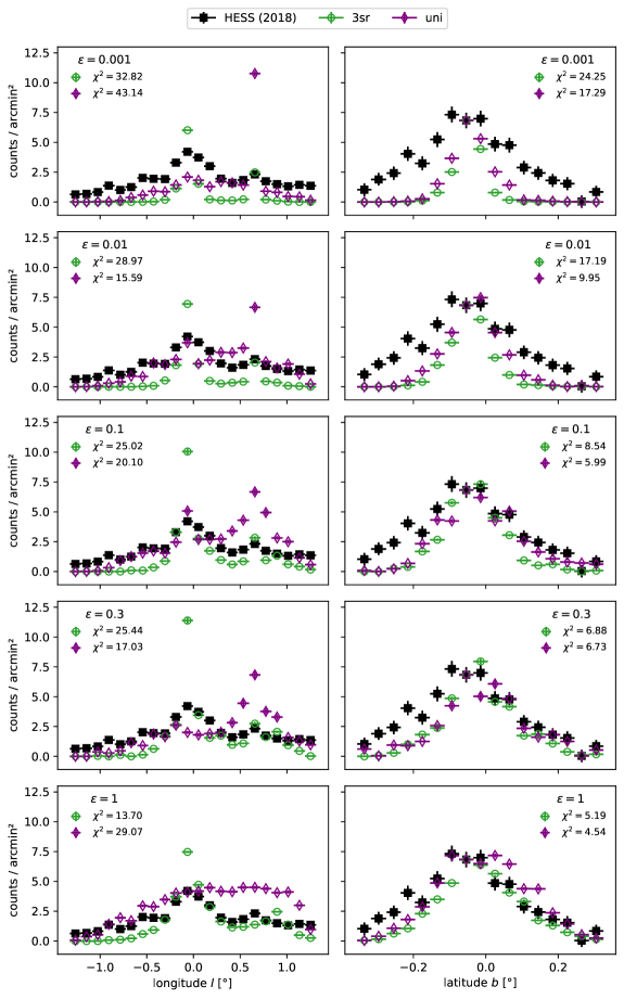
Figure 4: Profiles of the $\gamma$-ray distribution along the longitude (left column) and the latitude (right column). The row denotes the anisotropy parameter.

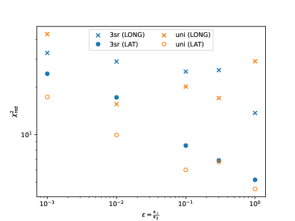
Figure 5: Reduced $\chi^{2}$ values to quantify the difference between the observed count profiles and the simulation (compare Fig. 4).

4.3 Spectra

Additional to the angular distribution of the $\gamma$-ray flux, also the spectral energy distribution (SED) is measured by H.E.S.S. (Abdalla et al., 2018), MAGIC (Acciari et al., 2020) and VERITAS (Adams et al., 2021). For this analysis, we consider different slopes of the CR injection spectrum $\left.\nicefrac{{\mathrm{d}N}}{{\mathrm{d}E}}\right|_{s}\sim E^{-\alpha_{s}}$. Indices in the range $1\leq\alpha_{s}\leq 3$ with steps of $\Delta\alpha_{s}=0.1$ are tested. For all configurations (source distribution, anisotropy of the diffusion tensor and source injection index) we bin the simulation data according to the H.E.S.S. observation, as they provide the finest energy resolution. The simulated SED is fitted with a power law

$$\Phi=\frac{\mathrm{d}N}{\mathrm{d}E}=\Phi_{0}\,\left(\frac{E}{1\,\mathrm{TeV}}\right)^{-\alpha}\quad,$$ (6)

where $\Phi_{0}$ is the normalisation at 1 TeV and $\alpha$ is the spectral index, and a power-law with exponential cut-off

$$\Phi=\Phi_{0}\,\left(\frac{E}{1\,\mathrm{TeV}}\right)^{-\alpha}\,\exp\left\{-\frac{E}{E_{c}}\right\}$$ (7)

with the cut-off energy $E_{c}$. The simulations allow in both cases for a free normalisation $\Phi_{0}$. Therefore, we choose the normalisation to minimise the $\chi^{2}$ difference between the fit and the observed data.

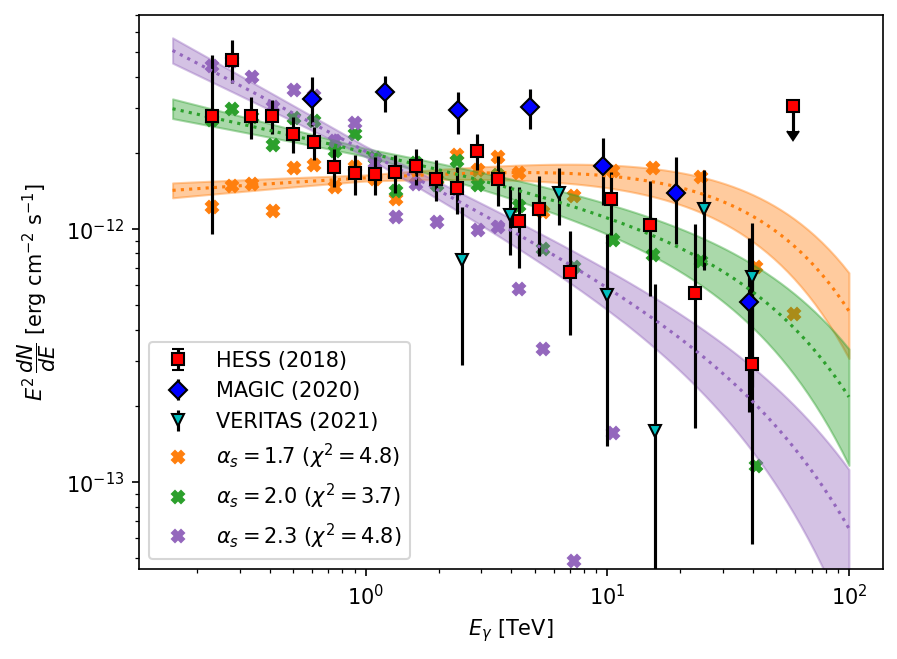
Figure 6: Example SED for the [3sr] source distribution and $\epsilon=0.1$. Three different injection slopes $\alpha_{s}$ are shown.

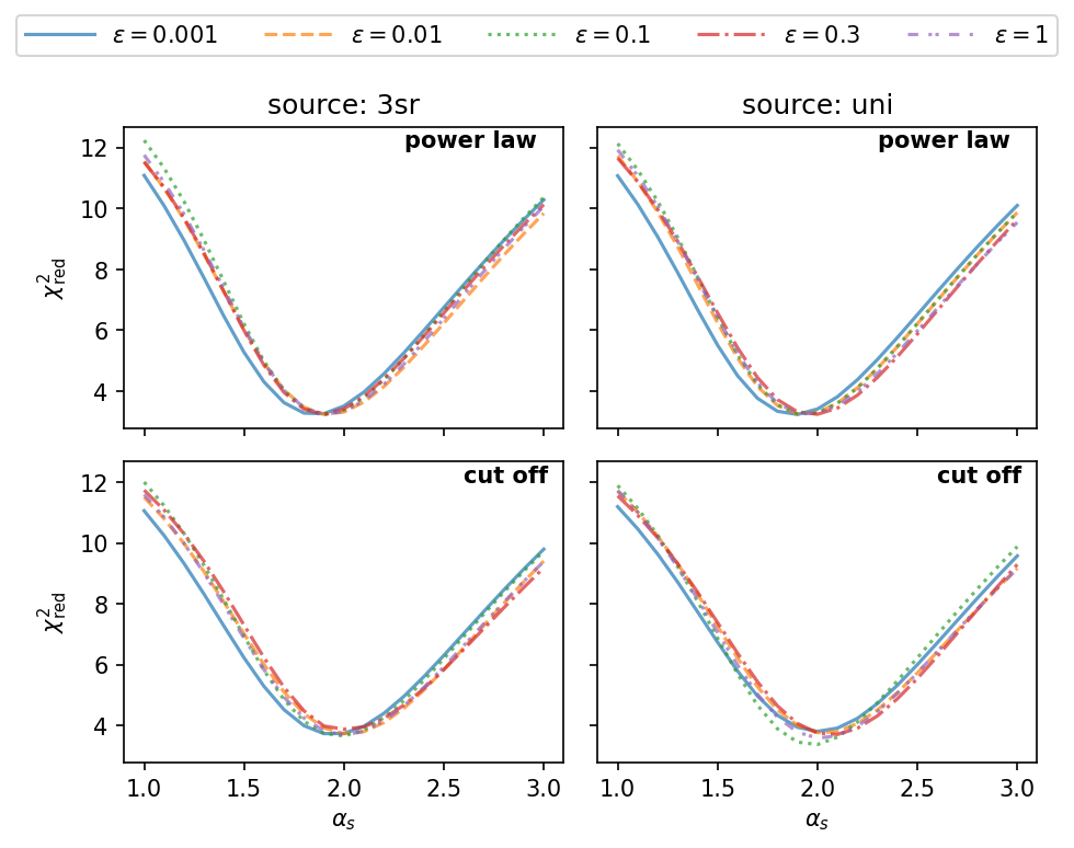
Figure 7: $\chi^{2}$ difference between the fitted SED and the observation depending on the source injection slope. The column indicates the spatial source distribution (left [3sr] , right [uni] ) and the row indicates the fitting function (upper: power law (eq. 6), lower: power law with cut-off (eq. 7)). The line color and style denotes different anisotropies of the diffusion tensor.

In Fig. 6 the SED is shown for the injection slope of $\alpha_{s}=1.7$ (orange), $\alpha_{s}=2.0$ (green) and $\alpha_{s}=2.3$ (purple) assuming the [3sr] spatial distribution and the anisotropy parameter of $\epsilon=0.1$ Also the observation by H.E.S.S. (Abdalla et al., 2018) (red squares), MAGIC (Acciari et al., 2020) (blue diamond) and VERITAS (Adams et al., 2021) (cyan triangle) are shown.

The results for the minimised $\chi^{2}$ based on the different injection slopes is shown in Fig. 7. All cases lead to a best fit for an injection slope $\alpha_{s}\approx 2$, while the pure power-law fit requires a slightly harder injection spectrum. The parameters for the best fits are summarised in table 2. No clear preference for the anisotropy parameter can be found for the SED fitting.

source	$\chi^{2}_{\mathrm{red}}$	$\epsilon$	$\alpha_{s}$	$\log_{10}\left(\Phi_{0}[\mathrm{TeV\,cm^{-2}\,s^{-1}}]\right)$	$\alpha$	$E_{c}$ [TeV]
[3sr]	$3.23$	$0.3$	$1.9$	$-11.705\pm 0.022$	$2.219\pm 0.028$	-
	$3.65$	$0.1$	$2.0$	$-11.692\pm 0.014$	$2.21\pm 0.03$	$79\pm 21$
[uni]	$3.23$	$0.001$	$1.9$	$-11.702\pm 0.019$	$2.233\pm 0.024$	-
	$3.37$	$0.1$	$2.0$	$-11.695\pm 0.008$	$2.250\pm 0.016$	$307\pm 169$

Table 2: Best fit parameter for the minimal $\chi^{2}_{\mathrm{red}}$ shown in Fig. 7. For both spatial models the first row corresponds to the power-law fit (eq. 6) and the second row to the cut-off fit (eq. 7).

5 Summary and Conclusion

Building a realistic three-dimensional model of the cosmic-ray (CR) transport inside the Central Molecular Zone (CMZ) requires detailed knowledge of the astrophysical environment, i.e. the gas distribution, the magnetic field configuration and the source positions.

In our work, we used the three-dimensional gas distribution from Ferrière et al. (2007). We adjusted the exponential scale height to $H_{c}=30\ \mathrm{pc}$ to match the observed thickness of the $\gamma$-ray emission. This value is near the upper limit of the observational uncertainties.

The anisotropy of the diffusion tensor $\epsilon=\kappa_{\perp}/\kappa_{\parallel}$, defined as the ratio between the diffusion perpendicular and parallel to the magnetic field line, is constrained by the observation of the longitudinal and latitudinal profiles and the SED of the $\gamma$-ray emission. The measurements by the H.E.S.S. telescopes (Abdalla et al., 2018) hint towards a nearly isotropic diffusion of CRs, while in the SED fitting no clear preference can be seen.

In this work we tested two different source scenarios, three different point sources within the CMZ and a global sea of old CRs from the Milky Way diffusing into the CMZ. The discrimination between the different source distributions and anisotropies is done best by comparing the longitudinal profiles. In this case the best agreement to the data could be achieved by the point source scenario. Here, the smallest $\chi^{2}_{\mathrm{red}}$ can be achieved. Only the position of the peak for positive longitudes is shifted a little bit outward. The distribution under predicts the outermost part. This might hint towards a missing gas target in this range or a contribution from the CR sea.

In general, the large-scale observables could be reproduced with our 3D model of the CMZ but some of the small-scale features are still missing. This is mainly due to the lack of substructures within the gas distribution, but also a more refined magnetic field model would be needed. This will become important with the upcoming next generation telescopes like CTA, which will provide a lower angular resolution and reveal more of these small-scale features.

Appendix A Estimating the maximal simulation time

To estimate the necessary total simulation time we test the number of particles left in the simulation volume in steps of $\Delta t=20\,\frac{\mathrm{kpc}}{c}$. This is done for all simulation setups with $N_{\mathrm{sim}}=10^{4}$ primaries.

In general the escape time is shorter for a less anisotropic diffusion. In Fig. 8 the fraction of particles in the simulation volume is shown as a function of time. Here the cases with $\epsilon=10^{-3}$ are chosen, to show the longest residence time. In both cases more than 99% of the particles left the volume before $t=100\frac{\mathrm{kpc}}{c}$. Therefore the total simulation time with $T_{\mathrm{max}}=500\frac{\mathrm{kpc}}{c}$ is even more conservative.

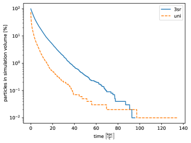
Figure 8: Number of particles left in the simulation volume.

Appendix B Raw data for 2D countmaps

In figure 9 the raw data for the synthetic $\gamma$-ray count maps are shown. The underlying binning uses $\Delta l=0.016^{\circ}$ and $\Delta b=0.01^{\circ}$. The simulation allows in principle for a finer binning but the statistics in each bin decreases. The bin size is chosen to minimize the noise, but keep the small-scale structures visible.

In the case of strong parallel transport, the small-scale structures of the magnetic field can be seen. For both source distributions the impact of the NTF called radio arc can bee seen. In the case of the [3sr] source distribution also smaller filaments in the region around Sgr A^∗ are visible.

For higher values of the isotropy parameter $\epsilon$ this effect is smeared out. For $\epsilon=0.01$ only the radio arc is visible for the [3sr] distribution by eye. In the other cases no small-scale structure appears.

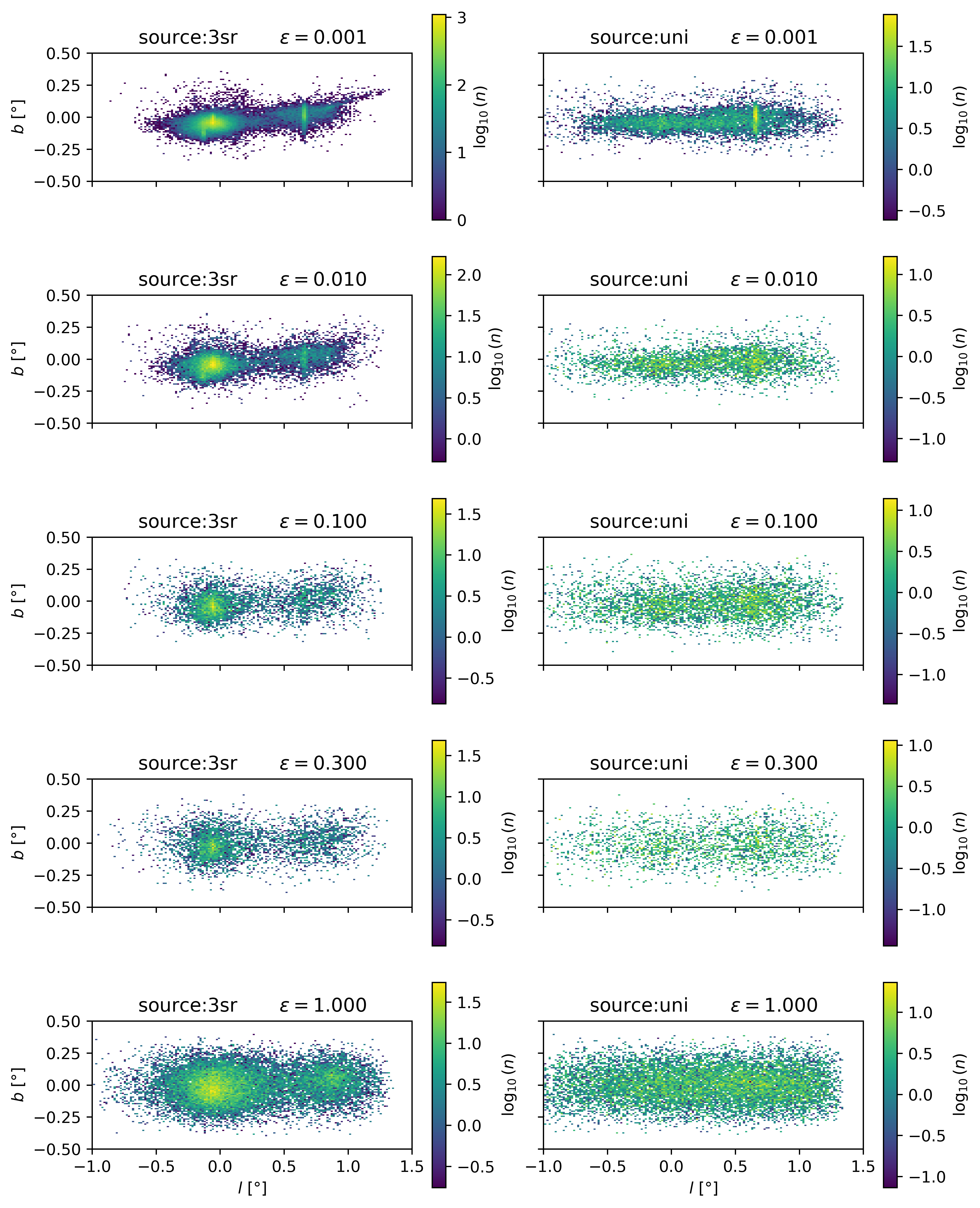
Figure 9: Synthetic $\gamma$-ray maps as shown in Fig. 3, but without a smearing for a PSF.

Appendix C Impact of source spectra on count profile

In section 4.2 the impact of the anisotropy on the resulting count profiles is shown. This analysis was only done for the case of a power-law injection with a slope $\alpha_{s}=2$. Here we show the difference for changing this index. In Fig. 10 the reduced $\chi^{2}$ values for different injection indices is shown. In the latitudinal profile the best fit value of $\epsilon=0.3$ stays for all injection indices. Only for the longitudinal profile the isotropic diffusion is preferred for indices $\alpha_{s}\geq 2.2$.

For the [uni] source distribution there are more changes with the injection index visible. But in all cases the intermediate anisotropy $\epsilon=0.1$ is still preferred in both profiles.

The general statement in sec. 4.2 does not change due to the choice of $\alpha_{s}=2.0$.

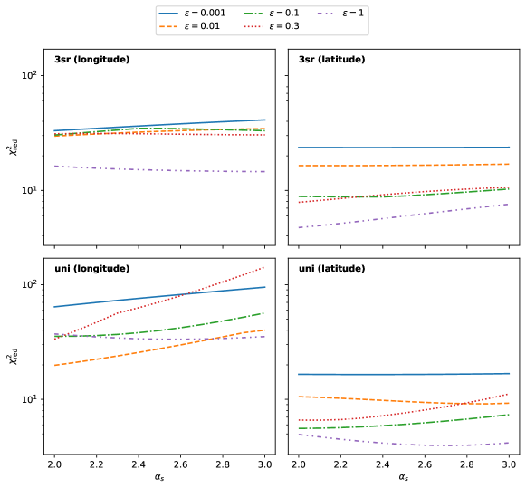
Figure 10: Impact of the source power law index $\alpha_{s}$ on the reduced $\chi^{2}$ difference between the simulation and the observed H.E.S.S. profile.

References

- Abbasi et al. (2023) Abbasi, R., Ackermann, M., Adams, J., et al. 2023, ApJ, 956, 20, doi: 10.3847/1538-4357/acf713
- Abdalla et al. (2018) Abdalla, H., Abramowski, A., Aharonian, F., et al. 2018, A&A, 612, A9, doi: 10.1051/0004-6361/201730824
- Abramowski et al. (2016) Abramowski, A., Aharonian, F., Benkhali, F. A., et al. 2016, Nature, 531, 476, doi: 10.1038/nature17147
- Acciari et al. (2020) Acciari, V. A., Ansoldi, S., Antonelli, L. A., et al. 2020, A&A, 642, A190, doi: 10.1051/0004-6361/201936896
- Ackermann et al. (2014) Ackermann, M., Albert, A., Atwood, W. B., et al. 2014, ApJ, 793, 64, doi: 10.1088/0004-637X/793/1/64
- Ackermann et al. (2017) Ackermann, M., Ajello, M., Albert, A., et al. 2017, ApJ, 840, 43, doi: 10.3847/1538-4357/aa6cab
- Adams et al. (2021) Adams, C. B., Benbow, W., Brill, A., et al. 2021, ApJ, 913, 115, doi: 10.3847/1538-4357/abf926
- Ajello et al. (2016) Ajello, M., Albert, A., Atwood, W. B., et al. 2016, ApJ, 819, 44, doi: 10.3847/0004-637X/819/1/44
- Batista et al. (2016) Batista, R. A., Dundovic, A., Erdmann, M., et al. 2016, J. Cosmology Astropart. Phys, 2016, 038, doi: 10.1088/1475-7516/2016/05/038
- Batista et al. (2022) Batista, R. A., Tjus, J. B., Dörner, J., et al. 2022, J. Cosmology Astropart. Phys, 2022, 035, doi: 10.1088/1475-7516/2022/09/035
- Becker Tjus & Merten (2020) Becker Tjus, J., & Merten, L. 2020, Phys. Rep., 872, 1, doi: 10.1016/j.physrep.2020.05.002
- Cao et al. (2023) Cao, Z., Aharonian, F., An, Q., et al. 2023, Physical Review Letters, 131, 151001, doi: 10.1103/PhysRevLett.131.151001
- Cerri et al. (2017) Cerri, S. S., Gaggero, D., Vittino, A., Evoli, C., & Grasso, D. 2017, J. Cosmology Astropart. Phys, 2017, 019, doi: 10.1088/1475-7516/2017/10/019
- Daylan et al. (2016) Daylan, T., Finkbeiner, D. P., Hooper, D., et al. 2016, Physics of the Dark Universe, 12, 1, doi: 10.1016/j.dark.2015.12.005
- Di Mauro (2021) Di Mauro, M. 2021, Phys. Rev. D, 103, 063029, doi: 10.1103/PhysRevD.103.063029
- Effenberger et al. (2012a) Effenberger, F., Fichtner, H., Scherer, K., et al. 2012a, ApJ, 750, 108, doi: 10.1088/0004-637X/750/2/108
- Effenberger et al. (2012b) Effenberger, F., Fichtner, H., Scherer, K., & Büsching, I. 2012b, A&A, 547, A120, doi: 10.1051/0004-6361/201220203
- Ferrière et al. (2007) Ferrière, K., Gillard, W., & Jean, P. 2007, A&A, 467, 611, doi: 10.1051/0004-6361:20066992
- Finkbeiner (2004) Finkbeiner, D. P. 2004, ApJ, 614, 186, doi: 10.1086/423482
- Goodenough & Hooper (2009) Goodenough, L., & Hooper, D. 2009, arXiv:0910.2998
- Guenduez et al. (2020) Guenduez, M., Becker Tjus, J., Ferrière, K., & Dettmar, R. J. 2020, A&A, 644, A71, doi: 10.1051/0004-6361/201936081
- H. E. S. S. Collaboration et al. (2018) H. E. S. S. Collaboration, Abdalla, H., Abramowski, A., et al. 2018, A&A, 612, A1, doi: 10.1051/0004-6361/201732098
- Harris et al. (2020) Harris, C. R., Millman, K. J., van der Walt, S. J., et al. 2020, Nature, 585, 357, doi: 10.1038/s41586-020-2649-2
- Henshaw et al. (2023) Henshaw, J. D., Barnes, A. T., Battersby, C., et al. 2023, in Astronomical Society of the Pacific Conference Series, Vol. 534, Protostars and Planets VII, 83, doi: 10.48550/arXiv.2203.11223
- Heywood et al. (2022) Heywood, I., Rammala, I., Camilo, F., et al. 2022, ApJ, 925, 165, doi: 10.3847/1538-4357/ac449a
- Hoerbe et al. (2020) Hoerbe, M. R., Morris, P. J., Cotter, G., & Becker Tjus, J. 2020, MNRAS, 496, 2885, doi: 10.1093/mnras/staa1650
- Hunter (2007) Hunter, J. D. 2007, Computing in Science & Engineering, 9, 90, doi: 10.1109/MCSE.2007.55
- Jokipii (1966) Jokipii, J. R. 1966, ApJ, 146, 480, doi: 10.1086/148912
- Kelner et al. (2006) Kelner, S. R., Aharonian, F. A., & Bugayov, V. V. 2006, Phys. Rev. D, 74, 034018, doi: 10.1103/PhysRevD.74.034018
- Merten et al. (2017) Merten, L., Becker Tjus, J., Fichtner, H., Eichmann, B., & Sigl, G. 2017, J. Cosmology Astropart. Phys, 2017, 046, doi: 10.1088/1475-7516/2017/06/046
- Pedlar et al. (1989) Pedlar, A., Anantharamaiah, K. R., Ekers, R. D., et al. 1989, ApJ, 342, 769, doi: 10.1086/167635
- Pérez & Granger (2007) Pérez, F., & Granger, B. E. 2007, Computing in Science and Engineering, 9, 21, doi: 10.1109/MCSE.2007.53
- Planck Collaboration et al. (2013) Planck Collaboration, Ade, P. A. R., Aghanim, N., et al. 2013, A&A, 554, A139, doi: 10.1051/0004-6361/201220271
- Reichherzer et al. (2020) Reichherzer, P., Becker Tjus, J., Zweibel, E. G., Merten, L., & Pueschel, M. J. 2020, MNRAS, 498, 5051, doi: 10.1093/mnras/staa2533
- Reichherzer et al. (2022a) Reichherzer, P., Becker Tjus, J., Zweibel, E. G., Merten, L., & Pueschel, M. J. 2022a, MNRAS, 514, 2658, doi: 10.1093/mnras/stac1408
- Reichherzer et al. (2022b) Reichherzer, P., Merten, L., Dörner, J., et al. 2022b, SN Applied Sciences, 4, 15, doi: 10.1007/s42452-021-04891-z
- Rocklin (2015) Rocklin, M. 2015, in Proceedings of the 14th Python in Science Conference, ed. K. Huff & J. Bergstra, 130 – 136
- Scherer et al. (2022) Scherer, A., Cuadra, J., & Bauer, F. E. 2022, A&A, 659, A105, doi: 10.1051/0004-6361/202142401
- Scherer et al. (2023) Scherer, A., Cuadra, J., & Bauer, F. E. 2023, A&A, 679, A114, doi: 10.1051/0004-6361/202245822
- Shalchi (2021) Shalchi, A. 2021, ApJ, 923, 209, doi: 10.3847/1538-4357/ac2363
- Sofue (2000) Sofue, Y. 2000, ApJ, 540, 224, doi: 10.1086/309297
- The CTA Consortium (2019) The CTA Consortium. 2019, Science with the Cherenkov Telescope Array (WORLD SCIENTIFIC), doi: 10.1142/10986
- Virtanen et al. (2020) Virtanen, P., Gommers, R., Oliphant, T. E., et al. 2020, Nature Methods, 17, 261, doi: 10.1038/s41592-019-0686-2
- Wes McKinney (2010) Wes McKinney. 2010, in Proceedings of the 9th Python in Science Conference, ed. Stéfan van der Walt & Jarrod Millman, 56 – 61, doi: 10.25080/Majora-92bf1922-00a